
Phenological Shifts of the Deciduous Forests and Their Responses to Climate Variations in North America


1
School of Remote Sensing and Information Engineering, Wuhan University, Wuhan 430079, China
2
Tourism School, Chuzhou University, Chuzhou 239000, China
*
Author to whom correspondence should be addressed.
Forests 2022, 13(7), 1137; https://doi.org/10.3390/f13071137
Submission received: 9 May 2022
/
Revised: 10 July 2022
/
Accepted: 16 July 2022
/
Published: 19 July 2022
(This article belongs to the Section Forest Ecology and Management)
Abstract
:Forests play a vital role in sequestering carbon dioxide from the atmosphere. Vegetation phenology is sensitive to climate changes and natural environments. Exploring the patterns in phenological events of the forests can provide useful insights for understanding the dynamics of vegetation growth and their responses to climate variations. Deciduous forest in North America is an important part of global forests. Here we apply time-series remote sensing imagery to map the critical dates of vegetation phenological events, including the start of season (SOS), end of season (EOS), and growth length (GL) of the deciduous forests in North America during the past two decades. The findings show that the SOS and EOS present considerable spatial and temporal variations. Earlier SOS, delayed EOS, and therefore extended GL are detected in a large part of the study area from temporal trend analysis over the years, though the magnitude of the trend varies at different locations. The phenological events are found to correlate to the environmental factors and the impact on the vegetation phenology from the factors is location-dependent. The findings confirm that the phenology of the deciduous forests in North America is updated such as advanced SOS and delayed EOS in the last two decades and the climate variations are likely among the driving forces for the updates. Considering that previous studies warn that shifts in vegetation phenology could reverse the role of forests as net emitters or net sinks, we suggest that forest management should be strengthened to forests that experience significant changes in the phenological events.
1. Introduction
Forests play a vital role in global carbon cycling. Forests sink the most carbon dioxide from the atmosphere and own the largest carbon pool compared to other terrestrial ecosystems such as grassland and cropland [1]. North America is one of the continents with a great part of the terrestrial lands covered by forests. Over the past few decades, the forest area in America has been reduced due to human activities [2,3]. The role of vegetation, including trees in forests, on the global environments is multifold. Vegetation sequesters carbon dioxide, and serves not only as a critical and irreplaceable biological pool, but also as a central hub for the interconnection between various spheres, including biosphere, hydrosphere, and atmosphere [4]. Studies for understanding the spatio-temporal vegetation dynamics have been carried out for a long time; those studies focus on a number of topics such as vegetation coverage, vegetation primary productivity, and vegetation landscape patterns, as well as the impact on the topics from climate changes and human activities [5,6]. Mapping the vegetation dynamics for forests is particularly important considering the contributions of forests to global carbon cycling [7].
Vegetation phenological events such as vegetation green-up, peak growth, leaf senescence and dormancy, are among the indicators to the ecological functions from vegetation [8]. Vegetation phenology can not only reflect switches in seasons or in a broader sense climate changes, but also open a window for understanding the mechanism for plants to adapt to the climate changes [9]. Vegetation phenology influences biomass productivity, biodiversity evolution, water balance and carbon balance at local, regional and global scales [10]. Previous studies show that the increase of temperature leads to significant advance of phenology in spring [11] and the delay of phenology in autumn [12], resulting in an extended plant growth season [13]. A few phenological events are within the study scope of vegetation phenology, including the start of growing season (SOS), the end of growing season (EOS) and the length of growing season [14]. For deciduous forests, the vegetation phenological events are often examined at an annual cycle and are subject to change under the influence of climatic and other environmental factors [15]. Vegetation in deciduous forests usually starts to turn green in spring, reaches peak greenness in summer and withers in autumn or early winter. However, vegetation phenological events are location-specific, as a result of the vegetation’s responses and adaptation to the environments [8,16]. Therefore, knowing the spatio-temporal patterns in vegetation phenology has both theoretical and practical implications for better managing ecosystems and understanding climate changes [17].
Several ways can be applied to make observations of vegetation phenology. Theoretically, the field-based observation is the most reliable method. For example, flux tower GPP time series data can be taken to examine the dynamics of vegetation phenology [18]. However, field-based observation is time consuming and labor intensive; it is thus not a cost-effective method to map vegetation phenology at multi-temporal points over a large area. Another difficulty from field-based observation is the determination of the phenological dates, which requires consistent standards or protocols. Unfortunately, such protocols are not widely accepted or even well documented, causing different phenological dates even from the same datasets when determined by different people at different times [10,19]. Such inconsistency in the vegetation phenology due to lack of agreed protocols could cause challenges in spatio-temporal pattern analysis on the phenology because the derived phenological dates may not be inter-comparable both spatially and temporally. Remote sensing has played an important role in understanding the temporal and spatial dynamic changes of plant phenology on a large scale [16]. Satellite remote sensing allows long-term observations on vegetation growth over a large area. Vegetation dynamics can be inversed from remote sensing imagery using vegetation indices such as the normalized distribution of vegetation index (NDVI). Once the identical protocols to extract the phenological events are applied to remotely sensed time-series imagery, it is possible to obtain spatio-temporally consistent phenological datasets for a large area and thus map the phenological dynamics from regional to global scales [20].
Forests are important to mitigate global warming. Out of all terrestrial ecosystems, forests absorb the largest part of carbon dioxide from the atmosphere as they grow and store the carbon in tree woods and soils [21,22]. Deciduous forests are characterized by typical vegetation growth cycles, including active growth in the spring, peak growth in the summer, leaf senescence in the autumn, and dormancy in the winter, and indicate to seasonal changes and climate variations. Thus, current work tries to understand the spatio-temporal patterns of the deciduous forests in North America in the past two decades (2001–2020) and explore the responses of the phenological events to the climate variations. We first use time-series NDVI data from remote sensing imagery to extract vegetation phenology of the deciduous forests. We then analyze the spatio-temporal patterns in the extracted dates of the phenological events and their dynamics against temperature and precipitation. The Google Earth Engine (GEE) platform allows efficient computation and mapping of the phenological events and their pattern analysis. The paper is organized as follows: the next section introduces the study area and data sources, the methodology will be presented in Section 3, the main findings are reported in Section 4, discussions and conclusion are given in Section 5 and Section 6, respectively.
2. Study Area and Data Sources
2.1. Study Area
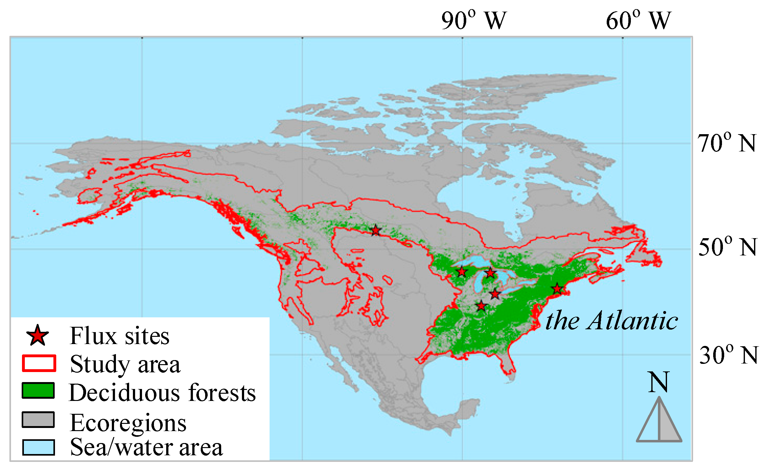
Deciduous forest is found in middle-latitude regions with a temperate climate characterized by a winter season. Deciduous forests are composed primarily of trees that grow and shed their leaves in an annual cycle. The phenology of deciduous forests is sensitive to climate changes and phenological shifts can bring substantial impacts on ecosystem function and services due to their large carbon pools and fluxes [23]. Changes in spring and autumn phenology of temperate plants in recent decades have become iconic bio-indicators of rapid climate change [24]. The land area of North America is broadly covered by level II regions that are nested within 15 level I ecological regions (www.epa.gov/eco-research/ecoregions-north-america, accessed on 1 May 2022) (Figure 1). The ecological regions at level II are useful for national and subcontinental overviews of ecological patterns. The land area, particularly in its eastern part, is one of the few regions that are characterized by deciduous forests. The response of vegetation phenology to climate changes has regional differences. Vegetation in mid-to-high latitudes (between 30–70° N) is particularly sensitive to climate changes [25]. We are therefore interested in the boundary of the area between latitudes between 30–70° N within the ecoregions of North America and with coverage of deciduous forests. We only selected the ecoregions that are related to forestry, including northern forests, northwestern forested mountains, marine west coast forest, and eastern temperate forests. To extract the coverage of the deciduous forests only, the land cover data from MODIS MCD12Q1 land cover data are used. The MCD12Q1 dataset applies the International Geosphere-Biosphere Programme classification protocol which divides the deciduous forests in the land cover types labeled as #3 (deciduous needleleaf forests) and #4 (deciduous broadleaf forests). All other land cover types are masked out. The deciduous forests are primarily in the eastern part of the study area, though they also scatter across the north and western regions (Figure 1).
2.2. Data Sources
Remote sensing technology provides an effective way to map vegetation growth, and thus SOS and EOS over a large-scale area. Multiple remote sensed datasets are applied to extract the forest phenology and the associated factors such as climatic variables. The time window covers the years from 2001 to 2020. All below mentioned raster datasets, if not at the scale of 500 m, are resampled to a resolution of 500 m.
One of the frequently adopted methods using remote sensing data to measure vegetation growth is through the normalized distribution of vegetation index (NDVI), which reflects the abundance of vegetation greenness [26]. For deciduous forests, NDVI starts to increase during the spring green-up, peaks in the full growth period, and decreases after the autumn dormancy. When multi-temporal NDVI imagery is collected for each year, the trajectory of the intensity of vegetation greenness can be analyzed against the days of the year, which allows to extract the phenological events. This study takes use of MOD13A1 (ver. 6.1) product, which provides NDVI at a per pixel basis at 500 m in spatial resolution and 16 days in temporal resolution.
Climate variations have been proved to affect vegetation phenology. To examine the impact from climate factors, we consider various climatic variables and soil properties, including summed annual precipitation (PREC), annual average temperature (AAT), vapor pressure deficit (VPD), monthly minimum temperature (MINT), monthly maximum temperature (MAXT), surface shortwave radiation (SSR), and soil moisture (SM). The climatic variables have been included in many light-use efficiency vegetation productivity models like Miami (PREC and AAT) [27] and CASA (PREC, MINT, MAXT, and SSR) [28]. In addition, VPD and SM are important to model water availability to vegetation growth. TerraClimate, derived from climatically aided interpolation by combining the WorldClim dataset and the CRU Ts4.0 dataset, has been widely applied for mapping regional and global ecological parameters [29], and is used to derive most of the variables, including PREC, MINT, MAXT, VPD, SSR, and SM. However, TerraClimate does not include AAT. Therefore, AAT used in this study comes from the fifth generation from the European Centre for Medium-Range Weather Forecasts reanalysis for the global climate and weather (https://www.ecmwf.int/en/era5-land, accessed on 3 May 2022), which provides one month per pixel atmosphere temperature at about 11 km spatial resolution.
To validate the phenological events from the remote sensing imager, the flux data from six site-based stations within the international flux network (FLUXNET, https://fluxnet.org/data, accessed on 12 March 2022) are collected to derive field-based results. The consistency between the field-based and the remotely sensed SOS and EOS is then evaluated. Each of the stations collects gross primary productivity for at least 5 years, with details shown in Table 1.
3. Methodology
3.1. Extraction of the Phenological Events
The annual NDVI curve against the date of year (DOY) provides important information for obtaining the dates of phenological events for both SOS and EOS. NDVI in the deciduous forests starts to increase in spring and decreases in autumn. The dates that the NDVI shows the fastest increase during the spring green-up and the fastest decline during autumn are usually believed to be the points that vegetation reaches the onsets of active growth and senescence. The MOD13A1 dataset can be taken to build such NDVI curves from the time-series observations made on the same location across a year. Theoretically, a standard NDVI curve in natural forests is smooth along the date of the year because it is very unlikely that forest vegetation presents abrupt changes without direct human interferences. However, noises could be introduced in the remotely sensed imagery and thus the NDVI product in areas where clouds and aerosols are present during satellite Earth observations from outer space [29]. Such noises must be removed as much as possible so that the NDVI curves can be smoothed along the day of year (DOY). There are several smoothing methods intended to minimize the data noises in NDVI, including the Savizky-Golay filter [30], mean iterative filter [31], and spline interpolation-sliding window average [19]. In this study, we use the Savitzky-Golay filtering method to denoise the NDVI data because it is easy to apply and capable of reconstructing a high-quality NDVI time-series data set [32]. The Savitzky-Golay method is a weighted moving average filtering method, which depends on a polynomial degree of least squares fitting within a window [33], and its calculation formula is as follows
where Y is the original NDVI value, Y* is the smoothed NDVI value, Ci is the coefficient or weight of the ith sample which can be obtained by least squares fitting from a given high-order polynomial, m is a parameter that determines the size of the moving window, and N (=2m + 1) is the sample size in the filtering window, Yj+i is the NDVI value for the i+jth sample, and j is the jth sample in the NDVI time series.
A cubic polynomial function is applied to interpolate the NDVI dataset. We first fit the function using the available NDIV points,
where Yt represents the NDVI for date t (t = 1, 16, 32, …) in DOY, a0~a3 are the polynomial coefficients which are fit using the least squares method from the available NDVI time series. After the coefficients of the function have been determined, NDVI for all dates in the year can be calculated.
The interpolated NDVI time series can be used to extract the dates of vegetation phenological events through threshold method [34], change point detection method [35], hybrid algorithm [14], or derivative analysis [10]. This study uses a dynamic threshold to extract the phenological events. The traditional threshold method predefines value to determine the phenological events. For example, when NDVI reaches a particular value in the spring season, the corresponding date is then assumed to be SOS. This method does not differentiate the vegetation status at various locations. Instead, a dynamic threshold method applies different threshold values to different locations. This dynamic threshold method considers both the maximum and minimum NDVI at a location, and is a location-dependent approach, which is more reasonable to obtain the threshold values [36]. For any given time-series NDVI curve representing the changes of vegetation growth within a year for a position, a location-dependent threshold is calculated as follows,
where NDVIsh indicates an NDVI threshold corresponding to the critical point for the SOS or EOS, NDVImax and NDVImin represent the maximum and minimum values of annual NDVI, respectively, the coefficient p is a ratio which is associated with vegetation cover types and is decided to be 0.5 [37], meaning both SOS and EOS are determined as the day in which the NDVI increases or drops at least 50% from the summer maximum. The date in DOY with NDVI reaching the location-dependent threshold is taken as SOS in spring or EOS in autumn for that particular location. Based on the SOS and EOS, the growing season length (GL) for the forests is defined as the total days between EOS and SOS. The three phenological events, including SOS, EOS and GL, are processed for each year during 2001–2020. To validate the result of the extracted SOS and EOS, the daily GPP data observed from the six flux stations (Table 1) are taken to derive the station-based phenological events, termed as photosynthesis phenology [38]. To make SOS and EOS from the two methods comparable, a similar extraction schema is adopted to compute the flux GPP, including Savizky-Golay filtering and dynamic threshold phenology extraction in which the coefficient p is set to be 0.15 [39], considering the difference of variables, i.e., NDVI from the remote sensed approach versus GPP from the flux stations. The SOS and EOS at the locations of the flux stations are extracted from the remote sensing approach and then compared with the results derived from the flux stations.
NDVIsh = (NDVImax − NDVImin) × p + NDVImin
3.2. Phenological Trend Analysis
The Theil-Sen median regression is widely used to make a trend analysis. It is a nonparametric estimator for fitting a line to a set of points that chooses the median of the slopes of all lines through pairs of two-dimensional sample points [40]. The Theil-Sen regression method has many advantages, which include but are not limited to no requirement for any distribution assumption, robustness to outliers, and simplicity in computation [40]. The outcome from Theil-Sen regression is the Sen’s slope which takes the form of,
where xj and xi (i = 1, 2, …, n−1, and j = 2, 3, …, n) represent the ith and jth sample in the time series, and Median is a function for selecting the median value from a set. When Sen’s slope is greater than 0, an increasing trend in the time-series data samples can be made, while a value less than 0 indicates a decreasing trend. The Sen’s slope provides a method to assess the magnitude of change in sequence of measurements in time.
We then use the Mann-Kendall significance test (M-K test) to check if the Sen’s slope derived from Equation (4) is statistically significant. The M-K trend test is a nonparametric method widely applied to compute trend analysis for climate changes [40]. Several steps are involved for the test. First, an S statistic is computed using,
and
where xi and xj represent time series data respectively, and n is the number of samples in the time series. The next step is to calculate the variance of S statistics and Z value in the forms of,
where n represents the number of samples in the time series data, g is the number of tied values, tp is the number of ties for pth value. A positive Z indicates an upward trend in the time series, and a negative Z indicates a negative trend. A |Z| ≥ 1.96 indicates that there is a significant trend in the time-series data where 1.96 is the critical value of Z1−α/2 for a probability value of 0.05 from the standard normal table [41].
3.3. Correlation Analysis between the Phenological Events and Climate Changes
The relationship between the extracted SOS, EOS, and GL and the explanatory climatic and soil variables, i.e., AAT, MINT, MAXT, PREC, SSR, VPD, and SM, was studied using correlation analysis. We aggregated each of the explanatory variables by averaging the monthly result into different time scales, including an annual step, an early season (from January to April) step, and a growing season step (from May to August), respectively. The partial Pearson correlation coefficient was then computed between the dates of each of the phenological events (SOS, EOS, or GL) and one of the aggregated explanatory variables with input samples from the years of 2001–2020.
4. Results
4.1. Spatio-Temporal Patterns in the Phenological Shifts
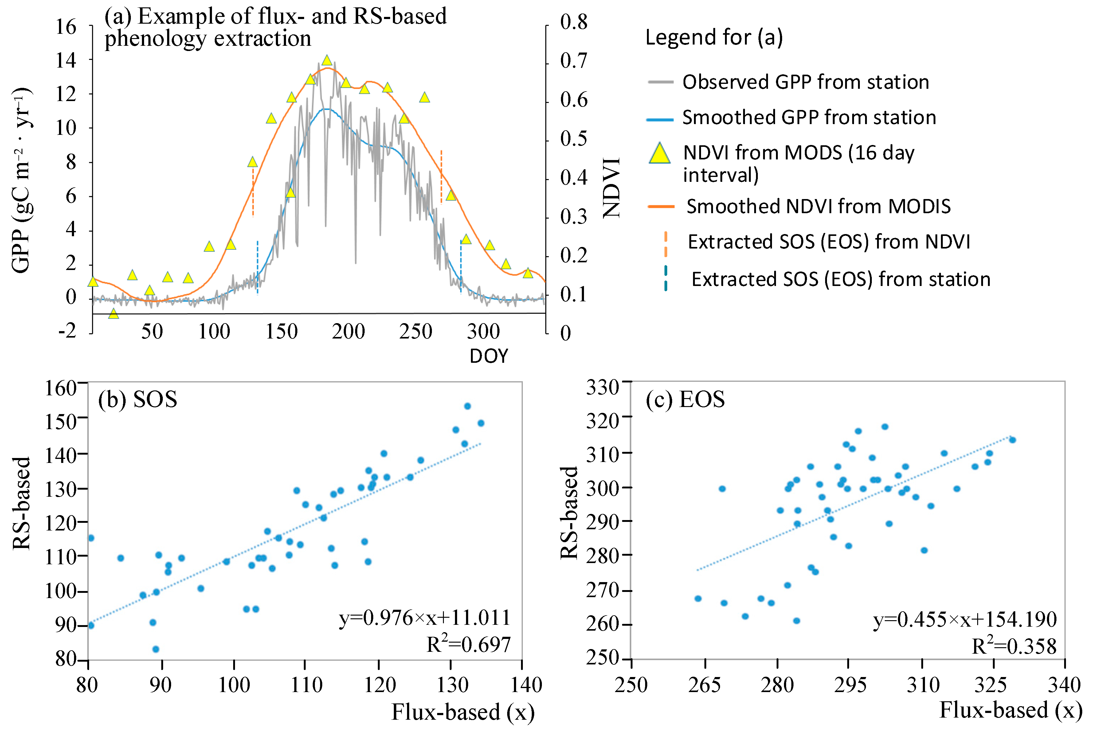
The SOS and EOS extracted from the remote sensing imagery (RS-based) and those from the flux stations (flux-based) are shown in Figure 2. The consistency between the flux-based and RS-based phenological events is shown in Figure 2a. Particularly, the coefficient of determination (R2) of the linear model for the SOS from the RS-based and flux-based methods reaches 0.697, suggesting that the SOS extracted from the remote sensing imagery is highly consistent with that from the flux observation (Figure 2b). The R2 (=0.358) in the linear model for the EOS shows a fair agreement between the EOS derived from the RS-based and flux-based methods (Figure 2c). Therefore, the dates extracted from the remote sensed imagery can largely indicate the seasonal growth cycles of the deciduous forests.
The mean and standard deviation (std) of the phenological events including SOS, EOS, and GL in the North American forests from 2001 to 2020 are presented in Figure 3. The spatially averaged SOS is 101.61 ± 11.04 DOY (Figure 3a), EOS is 304.26 ± 11.24 DOY (Figure 3c), and GL is 202.17 ± 19.34 days (Figure 3e). The green-up date indicated by the day of the year (DOY) generally presents an earlier trend along the latitude belts from the north to the south (Figure 3a). The EOS shows a more complex pattern; for example, the areas presenting earlier EOS mainly locate in the middle and the most northern parts of the study area, while the regions in the south and north-east tend to show relatively later EOS (Figure 3c). The SOS and EOS can have annual variations, due to many factors including climate fluctuations in the years. Both SOS and EOS show considerable temporal variations as reflected from the spatial distributions of the standard deviation (std) in both SOS and EOS (Figure 3b and Figure 4d); the SOS seems more sensitive to climate changes than EOS, as the SOS shows a larger annual variation than the EOS. The mean growth season length (GL), calculated based on the SOS to EOS of each year, shows a longer duration in the northwestern and southern parts of the study area (Figure 3e), with higher annual variation compared to those of SOS and EOS (Figure 3f).
In order to reveal the trend of the phenological events in the North American forests from 2001 to 2020, this study applied the model of Sen’s slope and the M-K test. Figure 4 shows the results from the Sen’s slope analysis and M-K test. The Sen’s slope in SOS indicates that majority of the study area presents negative values, suggesting an advanced or earlier green-up in the forests along the years (Figure 4a), while the positive values in the Sen’s slope for EOS indicate a delayed dormancy trend in the forests over the years (Figure 4c). Furthermore, the M-K test suggests that the trend in nearly half of those areas presenting advanced SOS or delayed EOS is statistically significant (Figure 4b and Figure 5d). The advanced SOS and delayed EOS result in a longer growing season of the vegetation (GL, from Figure S1), and thus may enable the forests to sequester more carbon from the atmosphere, which can be regarded as an adaptive response to the increased concentration of atmospheric CO2 [42].
4.2. The Impact of Temperature on the Phenological Shifts
Temperature is commonly considered to be one of the most important environmental factors affecting the forest phenological events for both SOS and EOS [43,44]. The impact from the annual average temperature (AAT) is shown in Figure 5. Most parts in the study area present a negative correlation between AAT and SOS, except a small area located in the eastern side where higher AAT seems to cause delayed SOS (Figure 5a). Furthermore, the significance test suggests that the advancing impact from higher AAT on SOS was significant for a large part of the study area (Figure 5b). The impact from AAT on EOS is spatially differentiated. In the northern part of the study area, EOS is negatively correlated to AAT, meaning higher AAT might advance EOS. In the middle and southern parts of the study area, mixed effects from AAT on EOS, i.e., advancing or delaying effect, were observed (Figure 5c), though such patterns are not significant for a great part of the area (Figure 5d). The update in the SOS and EOS from AAT results in prolonged length of vegetation growing season (GL) in a great part of the study area during the study period (Figure S2a,b).
4.3. The Impact of Precipitation on the Phenological Shifts
Precipitation (PREC) was previously proved to affect plant phenology [45]. At the same time, the water availability in soils is not only attributed to precipitation but also to soil properties [46], evapotranspiration [47], and landforms [48]. Thus, the sensitivity of the phenological events in the forests is even more spatially varied than that from the temperature changes. The impact from the annual precipitation is either positively or negatively correlated to SOS (Figure 6a), though such impact is not significant for most parts of the study areas (Figure 6b). The impact from PREC on EOS is positive in the southern part but mostly negative in the northern areas (Figure 6c), suggesting that more precipitation benefits later dormancy in the forests in the southern part of the study area while less precipitation favors later dormancy in the northern part. Similarly, the significance test shows that the impact from PREC on EOS is not consistently strong for most parts of the study area (Figure 6d). Overall, the changes in the SOS and EOS from PREC lead to a shortened length of the vegetation growing season (GL) (Figure S2c,d).
5. Discussions
5.1. The Phenological Events in the Deciduous Forests of North America
The current study examined vegetation green-up date, senescence date and growing season length (GL) in the deciduous forests of North America. The deciduous forests in North America primarily distribute in the eastern part, which is close to the Atlantic Ocean (Figure 1). On average, the SOS in the deciduous forests starts on 101.61 (±11.04) DOY while EOS occurs on 304.26 (±11.24) DOY. The higher long-term temporal variation of SOS than that in EOS (Figure 3b vs. Figure 3d) during the years suggests that SOS is more sensitive to contributing factors (e.g., precipitation and temperature) and thus may vary considerably because of the fluctuations in all attributed factors. The spatial variations of both SOS and EOS across the study area affect the growing season length (GL) of the vegetation. On average, GL exhibits 202.17 (±19.34) days, which is very close to the growing season length of forests at the global scale [49]. The SOS shows graded belts along the latitude, meaning that the forest vegetation presents earlier green-up from the north to the south along the belts because of the increasing temperature, though the spatial variations in the other climatic factors (e.g., precipitation and sun radiation) may explain the difference of the SOS in the same latitude belt. The EOS shows less spatial variations, but the spatial patterns reveal later vegetation dormancy in the north-eastern and southern parts of the study area than the middle area located far from the Atlantic Ocean. The temporal variations in the SOS, EOS, and GL suggest that EOS is the most stable phenological event in terms of the annual changes among the three indicators.
5.2. Modification of the Phenology in the Deciduous Forests from the Climate Variations
Temperature and precipitation are among the most important climate factors that can update vegetation phenology [24]. Vegetation needs soil water to support its growth and suitable temperature to trigger the physiological metabolism [7,50]. For a large-scale area like the one examined in this study that covers different latitudes and longitudes of the globe, the climate variables may differ considerably across locations. In addition, the study area meets the Atlantic Ocean on the eastern side and the inland climate could also be profoundly affected by the vast sea area (Figure 1). For example, the areas in the north-east and south-east part of the area present earlier SOS and later EOS. This study analyzes the impact from the environmental variables on the phenological events. The study indicates that AAT shows a consistent and homogeneous impact on SOS given that the majority of the area presents significantly advanced SOS. Furthermore, the higher temperature in the northern part of the study area shows an intensive impact on advancing the SOS. Though global warming is widely believed to advance SOS, the current study reveals that later SOS could be resulted from higher AAT in part of the eastern area close to the Atlantic Ocean (Figure 5a), which is in agreement with the finding that continued warming strengthens the effect of later fulfillment of chilling requirements and attenuates or even reverses the advancing trend in spring phenology [51]. Although warm springs led to an advance of the growing season, warm conditions in winter caused a delay of the spring phases [51].
The impact from annual PREC showed a more complex impact on the phenological events. Vegetation growth can be updated by the availability of soil water, which is not only attributed to precipitation but also to soil properties and landforms. The current study reveals that annual precipitation correlates to the phenological events, but the spatial patterns look rather heterogeneous, which could be resulted from the multiple factors contributing to water availability in soil that is essential to vegetation growth. Though precipitation is an important factor to soil water availability, we suggest that the impact from precipitation should be analyzed with combination of landforms and soil properties. Furthermore, nearby oceans influence regional climate conditions in several ways, including absorbing solar radiation and releasing heat, and/or updating aerosols that influence cloud covers [52], which may interact with precipitation to exert a joint effect on vegetation phenology.
The vegetation growing season length (GL) seems to be closely related to the adjacency to the Atlantic Ocean. The impact from the ocean favors GL, meaning the more closeness to the ocean, the earlier the SOS and later the EOS, and thus a longer growing season length for the vegetation in the forests. This finding supports the previous study that seas or oceans tend to minimize the climate variations [53], meaning the closeness to oceans would favor vegetation growth, and thus advance vegetation green-up and postpone vegetation dormancy.
In addition, we expect that other natural conditions may show impacts on the phenological events. Furthermore, environmental factors aggregated in different seasons (e.g., early growth season and growth season) rather than at an annual time step may present varied impact patterns. To highlight the different impact from the environmental variables, the correlation coefficients between the target (SOS, EOS, or GL) and the updated versions of the explanatory variables aggregated during January-April and May-August were computed and compared (Figure 7). In general, the temperature variables (AAT, MINT, and MAXT) show closer correlation to the phenological events under all the time spans, while the variables related to water availability including soil moisture (SM), water pressure deficit (VPD), and precipitation (PREC) show much less correlation to the phenological events. Surface shortwave radiation (SSR), which is an important factor to vegetation growth, also shows weak correlation to the target variables. Moreover, the environmental factors present a consistent impact on SOS and EOS, given the correlation coefficients with temperature variables (AAT, MINT, and MAXT) are all positive while such a pattern is reversed for GL at all the examined time spans. The findings probably suggest that temperature is the most important factor affecting the phenological events, either positively or negatively, while the other factors show less influence on the phenology of the deciduous forests in the study area.
5.3. Implications of the Shifts in the Phenological Events to Global Carbon Cycling
Global warming due to excessive carbon emissions has been reported and become a severe topic among scientists and governments in many countries of the world [42]. A continuous climbing of temperature seems to have caused and will continue to induce critical consequences to the safety of the global environments. The changes in vegetation phenology over a large area can not only indicate local climate changes but also send feedback to global carbon cycling [16]. Recent development in the remote sensing technology has made it possible to model large-scale spatio-temporal vegetation phenology, thanks to the availability of historically archived remote sensing datasets. When combined with climate datasets, it is more useful to understand the feedback of vegetation phenological events to global carbon cycling.
The current study confirms that the phenological events of the deciduous forests in North America have been greatly updated in the last two decades. Particularly, vegetation green-up dates have been advanced and vegetation dormancy postponed, which has prolonged the plant growing season. One benefit from a longer vegetation growth period is that it may allow forests to photosynthesize more carbon dioxide from the atmosphere, which partially neutralizes the excessively emitted carbon from human activities. However, the net effect from the extended growing season may vary from location to location, with consideration of the heterotrophic respiration from soil [54]. While extended growing season is believed to remove more atmospheric carbon in well-maintained forests, previous studies also pointed out that the soil respiration might overtake the increased amount of carbon absorption from photosynthesis in sparsely vegetation covered forests. For example, forests can emit more carbon than they absorb due to climate change; in southeastern Brazil, the dry and warm seasonal forests combined with gross deforestation were found to progressively absorb less carbon while releasing more over time [55]. From this perspective, the extended growing season length (GL) because of the changes in the SOS and EOS may result in two opposite results, either improved carbon sink or carbon source, depending on the vegetation cover and other environmental factors. However, forest management can help to realize a positive response from the forests, i.e., sequestering more carbon from the atmosphere in the context of the GL changes [56,57]. Therefore, we suggest special attention in terms of forest managements such as forest restoration and recovery programs be given to the areas that have presented a prolonged growing season period over the years (Figure 3e).
6. Conclusions
Forests play a vital role in global carbon cycling as they are the largest carbon pool and sink the majority of the carbon dioxide from the atmosphere [58]. The climate changes may alter the patterns of vegetation phenology and thus update the capacity of carbon sequestration from forests [59]. Understanding the spatio-temporal phenological patterns in forests in the context of global climate changes can provide valuable information for making decisions on forest management targeting improved carbon sequestration. The current study applies remotely sensed imagery to map the phenological events of the deciduous forests in North America and analyzes their spatio-temporal patterns in the last two decades, including the start of green-up season (SOS), end of growing season (EOS), and vegetation growing season length (GL). This study uses threshold algorithm to extract the phenological events by the Savitzky-Golay filtered NDVI, which are consistent with the results from the long-term flux monitoring sites, suggesting that the phenological events could be accurately extracted from remote sensed imagery when combined with appropriate phenology extraction methods. Some critical findings from the current work are summarized as follows,
- The start of growing season (SOS) or vegetation green-up dates represented by day of the year (DOY) of the deciduous forests is closely related to the latitude belts. The SOS increases along the belts from south to north, meaning vegetation green-up date becomes later in the more northern latitudes. Forests showing later end of growing season (EOS) and longer vegetation growth period are found to cluster in the north-eastern and southern parts of the study area.
- The SOS in the deciduous forests generally shows a significant advancing trend and EOS tends to delay to later DOY over the last two decades, resulting in substantial extension of the vegetation growing length (GL), which is likely to sink more carbon as a result of an adaptive response to the continuously rising concentration of carbon dioxide in the atmosphere.
- Vegetation phenology in the forests is closely correlated to climate variations in the study area. Higher annual average temperature (AAT) can lead to an earlier SOS. On the contrary, vegetation will wither earlier in lower latitude belts showing higher AAT, while delayed EOS is mainly observed in areas at higher latitude. The impact of precipitation on the phenological events shows as more spatially heterogeneous than that from AAT.
Though accumulated annual precipitation and annual average temperature are important climatic variables, temporal variation, e.g., monthly difference, in precipitation or temperature could discover a varied pattern in the relationships between climate fluctuation and vegetation phenology, which will be further examined. In addition to the climate factors such as AAT and precipitation, vegetation phenology in forests could be jointly affected by many other factors such as soil properties, landforms, and the closeness to oceans. The current study applies the Pearson’s correlation to examine the impact from each of the climate factors. In the future, advanced analytical models, such as partial least squares structural equation modeling [60], that incorporate all the above important factors in more detail in temporal granularity may be more effective to reveal each direct or their interaction impact on the vegetation phenological events (SOS, EOS, and/or GL) in the deciduous forests.
Supplementary Materials
The following supporting information can be downloaded at: https://www.mdpi.com/article/10.3390/f13071137/s1. Figure S1 Temporal trajectory of GL in the deciduous forests during 2001–2020; Figure S2 The impact of annual average temperature (AAT) and annual total precipitation (PREC) on GL in the deciduous forests.
Author Contributions
Conceptualization, Z.L. and Z.S.; methodology, H.F.; validation, H.F., Z.L. and J.T.; formal analysis, H.F.; investigation, X.L.; data curation, Z.L.; writing—original draft preparation, H.F.; writing—review and editing, Z.S.; visualization, Z.L.; funding acquisition, Z.S. All authors have read and agreed to the published version of the manuscript.
Funding
This work was supported in part by the National Natural Science Foundation of China (Nos. 41871296 and 42171447) and the Key Laboratory of Natural Resources Monitoring in Tropical and Subtropical Area of South China, Ministry of Natural Resources (No. 2022NRM006).
Institutional Review Board Statement
Not applicable.
Informed Consent Statement
Not applicable.
Data Availability Statement
Publicly available datasets were analyzed in this study. The MODIS and the climate variables can all be found from Google Earth Engine at https://earthengine.google.com, and the ecoregions of North America can be obtained at https://www.epa.gov/eco-research/ecoregions-north-america.
Conflicts of Interest
The authors declare no conflict of interest.
References
- Wu, C.; Gonsamo, A.; Gough, C.M.; Chen, J.M.; Xu, S. Modeling Growing Season Phenology in North American Forests Using Seasonal Mean Vegetation Indices from MODIS. Remote Sens. Environ. 2014, 147, 79–88. [Google Scholar] [CrossRef]
- Potapov, P.; Hansen, M.C.; Stehman, S.V.; Loveland, T.R.; Pittman, K. Combining MODIS and Landsat Imagery to Estimate and Map Boreal Forest Cover Loss. Remote Sens. Environ. 2008, 112, 3708–3719. [Google Scholar] [CrossRef]
- Mermoz, S.; Bouvet, A.; Koleck, T.; Ballère, M.; Le Toan, T. Continuous Detection of Forest Loss in Vietnam, Laos, and Cambodia Using Sentinel-1 Data. Remote Sens. 2021, 13, 4877. [Google Scholar] [CrossRef]
- Diaz, S.; Cabido, M. Plant functional types and ecosystem function in relation to global change. J. Veg. Sci. 1997, 8, 463–474. [Google Scholar] [CrossRef]
- Pandey, B.; Joshi, P.K.; Seto, K.C. Monitoring Urbanization Dynamics in India Using DMSP/OLS Night Time Lights and SPOT-VGT Data. Int. J. Appl. Earth Obs. Geoinf. 2013, 23, 49–61. [Google Scholar] [CrossRef]
- Smith, W.K.; Cleveland, C.C.; Reed, S.C.; Running, S.W. Agricultural Conversion without External Water and Nutrient Inputs Reduces Terrestrial Vegetation Productivity. Geophys. Res. Lett. 2014, 41, 449–455. [Google Scholar] [CrossRef] [Green Version]
- Montgomery, R.A.; Rice, K.E.; Stefanski, A.; Rich, R.L.; Reich, P.B. Phenological Responses of Temperate and Boreal Trees to Warming Depend on Ambient Spring Temperatures, Leaf Habit, and Geographic Range. Proc. Natl. Acad. Sci. USA 2020, 117, 10397–10405. [Google Scholar] [CrossRef]
- Verbesselt, J.; Hyndman, R.; Newnham, G.; Culvenor, D. Detecting Trend and Seasonal Changes in Satellite Image Time Series. Remote Sens. Environ. 2010, 114, 106–115. [Google Scholar] [CrossRef]
- Saxena, K.G.; Rao, K.S. Climate Change and Vegetation Phenology; Springer: Singapore, 2020; ISBN 10.1007/9789811. [Google Scholar]
- Sha, Z.; Zhong, J.; Bai, Y.; Tan, X.; Li, J. Spatio-Temporal Patterns of Satellite-Derived Grassland Vegetation Phenology from 1998 to 2012 in Inner Mongolia, China. J. Arid Land 2016, 8, 462–477. [Google Scholar] [CrossRef] [Green Version]
- Zheng, J.; Ge, Q.; Zhao, H. Changes of Plant Phenological Period and Its Response to Climate Change for the Last 40 Years in China. Agrometeorol. China 2003, 24, 28–32. [Google Scholar]
- Lu, P.; Yu, Q.; He, Q. Responses of Plant Phenology to Climatic Change. ACTA Ecol. Sin. 2006, 26, 923–929. [Google Scholar]
- Fu, Y.; Li, X.; Zhou, X.; Geng, X.; Guo, Y.; Zhang, Y. Progress in Plant Phenology Modeling under Global Climate Change. Sci. China Earth Sci. 2020, 50, 1206–1218. [Google Scholar] [CrossRef]
- Gonsamo, A.; Chen, J.M.; David, T.P.; Kurz, W.A.; Wu, C. Land Surface Phenology from Optical Satellite Measurement and CO2 Eddy Covariance Technique. J. Geophys. Res. Biogeosci. 2012, 117, 1–18. [Google Scholar] [CrossRef]
- Jeganathan, C.; Dash, J.; Atkinson, P.M. Remotely Sensed Trends in the Phenology of Northern High Latitude Terrestrial Vegetation, Controlling for Land Cover Change and Vegetation Type. Remote Sens. Environ. 2014, 143, 154–170. [Google Scholar] [CrossRef]
- Liu, Z.; Wu, C.; Liu, Y.; Wang, X.; Fang, B.; Yuan, W.; Ge, Q. Spring Green-up Date Derived from GIMMS3g and SPOT-VGT NDVI of Winter Wheat Cropland in the North China Plain. ISPRS J. Photogramm. Remote Sens. 2017, 130, 81–91. [Google Scholar] [CrossRef]
- Fang, J.; Piao, S.; He, J.; Ma, W. Increasing terrestrial vegetation activity in China, 1982–1999. Sci. China Ser. C Life Sci. 2004, 47, 229–240. [Google Scholar]
- Zhang, J.; Tong, X.; Zhang, J.; Meng, P.; Li, J.; Liu, P. Dynamics of Phenology and Its Response to Climatic Variables in a Warm-Temperate Mixed Plantation. For. Ecol. Manag. 2021, 483, 118785. [Google Scholar] [CrossRef]
- Cong, N.; Wang, T.; Nan, H.; Ma, Y.; Wang, X.; Myneni, R.B.; Piao, S. Changes in Satellite-Derived Spring Vegetation Green-up Date and Its Linkage to Climate in China from 1982 to 2010: A Multimethod Analysis. Glob. Chang. Biol. 2013, 19, 881–891. [Google Scholar] [CrossRef]
- White, M.A.; Thornton, P.E.; Running, S.W. A Continental Phenology Model for Monitoring Vegetation Responses to Interannual Climatic Variability. Glob. Biogeochem. Cycles 1997, 11, 217–234. [Google Scholar] [CrossRef]
- Prieto-Blanco, A.; North, P.R.J.; Barnsley, M.J.; Fox, N. Satellite-Driven Modelling of Net Primary Productivity (NPP): Theoretical Analysis. Remote Sens. Environ. 2009, 113, 137–147. [Google Scholar] [CrossRef]
- Schwartz, N.B.; Uriarte, M.; Defries, R.; Gutierrez-Velez, V.H.; Pinedo-Vasquez, M.A. Land-Use Dynamics Influence Estimates of Carbon Sequestration Potential in Tropical Second-Growth Forest. Environ. Res. Lett. 2017, 12, 7. [Google Scholar] [CrossRef]
- Xie, Y.; Wilson, A.M. Change Point Estimation of Deciduous Forest Land Surface Phenology. Remote Sens. Environ. 2020, 240, 111698. [Google Scholar] [CrossRef]
- Xie, Y.; Wang, X.; Silander, J.A. Deciduous Forest Responses to Temperature, Precipitation, and Drought Imply Complex Climate Change Impacts. Proc. Natl. Acad. Sci. USA 2015, 112, 13585–13590. [Google Scholar] [CrossRef] [PubMed] [Green Version]
- Song, Y.; Zajic, C.J.; Hwang, T.; Hakkenberg, C.R.; Zhu, K. Widespread Mismatch Between Phenology and Climate in Human-Dominated Landscapes. AGU Adv. 2021, 2, e2021AV000431. [Google Scholar] [CrossRef]
- Miao, L.; Luan, Y.; Luo, X.; Liu, Q.; Moore, J.C.; Nath, R.; He, B.; Zhu, F.; Cui, X. Analysis of the Phenology in the Mongolian Plateau by Inter-Comparison of Global Vegetation Datasets. Remote Sens. 2013, 5, 5193–5208. [Google Scholar] [CrossRef] [Green Version]
- Zaks, D.P.M.; Ramankutty, N.; Barford, C.C.; Foley, J.A. From Miami to Madison: Investigating the Relationship between Climate and Terrestrial Net Primary Production. Glob. Biogeochem. Cycles 2007, 21, GB3004. [Google Scholar] [CrossRef] [Green Version]
- He, C.; Liu, Z.; Xu, M.; Ma, Q.; Dou, Y. Urban Expansion Brought Stress to Food Security in China: Evidence from Decreased Cropland Net Primary Productivity. Sci. Total Environ. 2017, 576, 660–670. [Google Scholar] [CrossRef]
- Cao, P.; Zhang, L.; Li, S.; Zhang, J. Review on Vegetation Phenology Observation and Phenological Index Extraction. Adv. Earth Sci. 2016, 31, 365–376. [Google Scholar] [CrossRef]
- Hird, J.N.; McDermid, G.J. Noise reduction of NDVI time series: An empirical comparison of selected techniques. Remote Sens. Environ. 2009, 113, 248–258. [Google Scholar] [CrossRef]
- Ma, M.; Veroustraete, F. Reconstructing Pathfinder AVHRR Land NDVI Time-Series Data for the Northwest of China. Adv. Sp. Res. 2006, 37, 835–840. [Google Scholar] [CrossRef]
- Chen, J.; Jönsson, P.; Tamura, M.; Gu, Z.; Matsushita, B.; Eklundh, L. A Simple Method for Reconstructing a High-Quality NDVI Time-Series Data Set Based on the Savitzky--Golay Filter. Remote Sens. Environ. 2004, 91, 332–344. [Google Scholar] [CrossRef]
- Li, N.; Zhan, P.; Pan, Y.; Zhu, X.; Li, M.; Zhang, D. Comparison of remote sensing time-series smoothing methods for grassland spring phenology extraction on the Qinghai–Tibetan plateau. Remote Sens. 2020, 12, 3383. [Google Scholar] [CrossRef]
- White, M.A.; de Beurs, K.M.; Didan, K.; Inouye, D.W.; Richardson, A.D.; Jensen, O.P.; O’Keefe, J.; Zhang, G.; Nemani, R.R.; van Leeuwen, W.J.D.; et al. Intercomparison, Interpretation, and Assessment of Spring Phenology in North America Estimated from Remote Sensing for 1982–2006. Glob. Chang. Biol. 2009, 15, 2335–2359. [Google Scholar] [CrossRef]
- Zhang, X.; Friedl, M.A.; Schaaf, C.B.; Strahler, A.H.; Hodges, J.C.F.; Gao, F.; Reed, B.C.; Huete, A. Monitoring Vegetation Phenology Using MODIS. Remote Sens. Environ. 2003, 84, 471–475. [Google Scholar] [CrossRef]
- Wu, C.; Gough, C.M.; Chen, J.M.; Gonsamo, A. Evidence of Autumn Phenology Control on Annual Net Ecosystem Productivity in Two Temperate Deciduous Forests. Ecol. Eng. 2013, 60, 88–95. [Google Scholar] [CrossRef]
- Cong, N.; Piao, S.; Chen, A.; Wang, X.; Lin, X.; Chen, S.; Han, S.; Zhou, G.; Zhang, X. Spring Vegetation Green-up Date in China Inferred from SPOT NDVI Data: A Multiple Model Analysis. Agric. For. Meteorol. 2012, 165, 104–113. [Google Scholar] [CrossRef]
- D’Odorico, P.; Gonsamo, A.; Gough, C.M.; Bohrer, G.; Morison, J.; Wilkinson, M.; Hanson, P.J.; Gianelle, D.; Fuentes, J.D.; Buchmann, N. The Match and Mismatch between Photosynthesis and Land Surface Phenology of Deciduous Forests. Agric. For. Meteorol. 2015, 214, 25–38. [Google Scholar] [CrossRef]
- Wang, X.; Xiao, J.; Li, X.; Cheng, G.; Ma, M.; Zhu, G.; Altaf Arain, M.; Andrew Black, T.; Jassal, R.S. No Trends in Spring and Autumn Phenology during the Global Warming Hiatus. Nat. Commun. 2019, 10, 2389. [Google Scholar] [CrossRef]
- Wang, H.; Dai, J.; Rutishauser, T.; Gonsamo, A.; Wu, C.; Ge, Q. Trends and Variability in Temperature Sensitivity of Lilac Flowering Phenology. J. Geophys. Res. Biogeosci. 2018, 123, 807–817. [Google Scholar] [CrossRef] [Green Version]
- Ahmad, I.; Tang, D.; Wang, T.; Wang, M.; Wagan, B. Precipitation Trends over Time Using Mann-Kendall and Spearman’s Rho Tests in Swat River Basin, Pakistan. Adv. Meteorol. 2015, 2015, 431860. [Google Scholar] [CrossRef] [Green Version]
- Peters, G.P.; Andrew, R.M.; Canadell, J.G.; Friedlingstein, P.; Jackson, R.B.; Korsbakken, J.I.; Le Quéré, C.; Peregon, A. Carbon Dioxide Emissions Continue to Grow amidst Slowly Emerging Climate Policies. Nat. Clim. Chang. 2020, 10, 3–6. [Google Scholar] [CrossRef]
- Suonan, J.; Classen, A.T.; Sanders, N.J.; He, J.S. Plant Phenological Sensitivity to Climate Change on the Tibetan Plateau and Relative to Other Areas of the World. Ecosphere 2019, 10, e02543. [Google Scholar] [CrossRef]
- Gordo, O.; Sanz, J.J. Impact of Climate Change on Plant Phenology in Mediterranean Ecosystems. Glob. Chang. Biol. 2010, 16, 1082–1106. [Google Scholar] [CrossRef]
- Jin, H.; Jönsson, A.M.; Olsson, C.; Lindström, J.; Jönsson, P.; Eklundh, L. New Satellite-Based Estimates Show Significant Trends in Spring Phenology and Complex Sensitivities to Temperature and Precipitation at Northern European Latitudes. Int. J. Biometeorol. 2019, 63, 763–775. [Google Scholar] [CrossRef] [PubMed] [Green Version]
- Rawls, W.J.; Brakensiek, D.L. Estimating Soil Water Retention from Soil Properties. J. Irrig. Drain. Div. 1982, 108, 166–171. [Google Scholar] [CrossRef]
- Ajjur, S.B.; Al-Ghamdi, S.G. Evapotranspiration and Water Availability Response to Climate Change in the Middle East and North Africa. Clim. Chang. 2021, 166, 28. [Google Scholar] [CrossRef]
- Siqueira, D.S.; Marques, J.; Pereira, G.T. The Use of Landforms to Predict the Variability of Soil and Orange Attributes. Geoderma 2010, 155, 55–66. [Google Scholar] [CrossRef]
- Johnson, C.M.; J.Zarin, D.; H.Johnson, A. Post-Disturbance Aboveground Biomass Accumulation in Global Secondary Forests. Ecology 2000, 81, 1395–1401. [Google Scholar] [CrossRef]
- Li, S.; Yang, Y.; Zhang, Q.; Liu, N.; Xu, Q.; Hu, L. Differential Physiological and Metabolic Response to Low Temperature in Two Zoysiagrass Genotypes Native to High and Low Latitude. PLoS ONE 2018, 13, e0198885. [Google Scholar] [CrossRef]
- Yu, H.; Luedeling, E.; Xu, J. Winter and Spring Warming Result in Delayed Spring Phenology on the Tibetan Plateau. Proc. Natl. Acad. Sci. USA 2010, 107, 22151–22156. [Google Scholar] [CrossRef] [Green Version]
- Gao, K.; Beardall, J.; Häder, D.P.; Hall-Spencer, J.M.; Gao, G.; Hutchins, D.A. Effects of Ocean Acidification on Marine Photosynthetic Organisms under the Concurrent Influences of Warming, UV Radiation, and Deoxygenation. Front. Mar. Sci. 2019, 6, 322. [Google Scholar] [CrossRef]
- Scott-Buechler, C.M.; Greene, C.H. Role of the ocean in climate stabilization. In Bioenergy with Carbon Capture and Storage: Using Natural Resources for Sustainable Development; Academic Press: Cambridge, MA, USA, 2019; pp. 109–130. ISBN 9780128162293. [Google Scholar]
- Velasco, E.; Roth, M.; Norford, L.; Molina, L.T. Does Urban Vegetation Enhance Carbon Sequestration? Landsc. Urban Plan. 2016, 148, 99–107. [Google Scholar] [CrossRef]
- Maia, V.A.; Santos, A.B.M.; de Aguiar-Campos, N.; de Souza, C.R.; de Oliveira, M.C.F.; Coelho, P.A.; Morel, J.D.; da Costa, L.S.; Farrapo, C.L.; Fagundes, N.C.A.; et al. The Carbon Sink of Tropical Seasonal Forests in Southeastern Brazil Can Be under Threat. Sci. Adv. 2020, 6, eabd4548. [Google Scholar] [CrossRef] [PubMed]
- Schröder, W.; Pesch, R. Mapping Carbon Sequestration in Forests at the Regional Scale—A Climate Biomonitoring Approach by Example of Germany. Environ. Sci. Eur. 2011, 23, 31. [Google Scholar] [CrossRef] [Green Version]
- Zhou, H.; Van Rompaey, A.; Wang, J. Detecting the Impact of the “Grain for Green” Program on the Mean Annual Vegetation Cover in the Shaanxi Province, China Using SPOT-VGT NDVI Data. Land Use Policy 2009, 26, 954–960. [Google Scholar] [CrossRef]
- Dixon, R.K.; Brown, S.; Houghton, R.A.; Solomon, A.M.; Trexler, M.C.; Wisniewski, J. Carbon Pools and Flux of Global Forest Ecosystems. Science 1994, 263, 185–190. [Google Scholar] [CrossRef]
- Yu, L.; Yan, Z.; Zhang, S. Forest Phenology Shifts in Response to Climate Change over China–Mongolia–Russia International Economic Corridor. Forests 2020, 11, 757. [Google Scholar] [CrossRef]
- Sha, Z.; Xie, Y.; Tan, X.; Bai, Y.; Li, J.; Liu, X. Assessing the Impacts of Human Activities and Climate Variations on Grassland Productivity by Partial Least Squares Structural Equation Modeling (PLS-SEM). J. Arid Land 2017, 9, 473–488. [Google Scholar] [CrossRef]
Figure 1.
The study area of North America. Deciduous forests are extracted from MODIS MCD12Q1 for the year of 2020.
Figure 1.
The study area of North America. Deciduous forests are extracted from MODIS MCD12Q1 for the year of 2020.

Figure 2.
Comparison of the dates of the phenological events (SOS and EOS) extracted from remote sensing imagery (RS-based) and from the flux stations (flux-based). The flux-based and RS-based events are exampled (for site-id US-UMB) in (a) and each point in (b,c) denotes the SOS (or EOS) in day of year (DOY) from the RS-based and flux-based methods for an identical location and year.

Figure 3.
Spatial patterns of the phenological events in the North American deciduous forest from 2001 to 2020. Spatially averaged SOS is 101.61 ± 11.04 (a), EOS is 304.26 ± 11.24 (c), and GL is 202.17 ± 19.34 (e).
Figure 3.
Spatial patterns of the phenological events in the North American deciduous forest from 2001 to 2020. Spatially averaged SOS is 101.61 ± 11.04 (a), EOS is 304.26 ± 11.24 (c), and GL is 202.17 ± 19.34 (e).

Figure 4.
Temporal trajectory of the phenological events (SOS and EOS) in the deciduous forests during 2001–2020.
Figure 4.
Temporal trajectory of the phenological events (SOS and EOS) in the deciduous forests during 2001–2020.

Figure 5.
The impact of annual average temperature (AAT) on the phenological events (SOS and EOS) in the deciduous forests.
Figure 5.
The impact of annual average temperature (AAT) on the phenological events (SOS and EOS) in the deciduous forests.

Figure 6.
The impact of the annual total precipitation (PREC) on the phenological events in the deciduous forests.
Figure 6.
The impact of the annual total precipitation (PREC) on the phenological events in the deciduous forests.

Figure 7.
Correlation coefficient between the environmental variables, at different time intervals, and the phenological events in the deciduous forests. The x-axle indicates the correlation coefficient between the phenological event given in the sub-title and a variable, where the label N for the variable indicates a negative correlation. Updated versions means different time intervals, including time windows from January to April, from May to August, and whole year (annual), for (1) SSR, (2) SM, (3) VPD, (4) AAT, (5) MAXT, (6) MINT and (7) PREC.


Table 1.
Detail information of the flux sites.
| Site Id | Site Name | Latitude | Longitude | Elevation (m) | Time Window |
|---|---|---|---|---|---|
| CA-Oas | Saskatchewan—Western Boreal, Mature Aspen | 53.629 | −106.198 | 530 | 2001–2010 |
| US-MMS | Morgan Monroe State Forest | 39.323 | −86.413 | 275 | 2001–2010 |
| US-UMB | Univ. of Mich. Biological Station | 45.560 | −84.714 | 234 | 2001–2010 |
| US-Oho | Oak Openings | 41.554 | −83.844 | 230 | 2004–2006, 2008–2010 |
| US-WCr | Willow Creek | 45.806 | −90.080 | 520 | 2001–2003, 2005–2009 |
| US-Ha1 | Harvard Forest EMS Tower | 42.538 | −72.172 | 340 | 2002, 2005, 2007–2010 |
Publisher’s Note: MDPI stays neutral with regard to jurisdictional claims in published maps and institutional affiliations. |
© 2022 by the authors. Licensee MDPI, Basel, Switzerland. This article is an open access article distributed under the terms and conditions of the Creative Commons Attribution (CC BY) license (https://creativecommons.org/licenses/by/4.0/).
Share and Cite
MDPI and ACS Style
Li, Z.; Fang, H.; Tu, J.; Li, X.; Sha, Z. Phenological Shifts of the Deciduous Forests and Their Responses to Climate Variations in North America. Forests 2022, 13, 1137. https://doi.org/10.3390/f13071137
AMA Style
Li Z, Fang H, Tu J, Li X, Sha Z. Phenological Shifts of the Deciduous Forests and Their Responses to Climate Variations in North America. Forests. 2022; 13(7):1137. https://doi.org/10.3390/f13071137
Chicago/Turabian StyleLi, Zixuan, Husheng Fang, Jianguang Tu, Xiaolei Li, and Zongyao Sha. 2022. "Phenological Shifts of the Deciduous Forests and Their Responses to Climate Variations in North America" Forests 13, no. 7: 1137. https://doi.org/10.3390/f13071137
Note that from the first issue of 2016, this journal uses article numbers instead of page numbers. See further details here.