Article

Combination Strategies of Variables with Various Spatial Resolutions Derived from GF-2 Images for Mapping Forest Stock Volume

1
Research Center of Forestry Remote Sensing & Information Engineering, Central South University of Forestry and Technology, Changsha 410004, China
2
Key Laboratory of Forestry Remote Sensing Based Big Data & Ecological Security for Hunan Province, Changsha 410004, China
3
Key Laboratory of State Forestry Administration on Forest Resources Management and Monitoring in Southern Area, Changsha 410004, China
*
Authors to whom correspondence should be addressed.
Forests 2023, 14(6), 1175; https://doi.org/10.3390/f14061175
Submission received: 4 April 2023 / Revised: 23 May 2023 / Accepted: 2 June 2023 / Published: 6 June 2023
(This article belongs to the Special Issue Forestry Remote Sensing: Biomass, Changes and Ecology)

Abstract

:
Spectral features (SFs) and texture features (TFs) extracted from optical remote sensing images can capture the structural composition and growth information of forests, and combining remote sensing variables with a few ground measurement samples is a common method for mapping forest stock volume (FSV). However, the accuracy of mapping FSV using optical images with a high spatial resolution (one meter or sub-meters) is often lower than medium resolutions (larger than 10 m) using the same types of features and approaches. To overcome the limitations of high spatial resolution images in mapping FSV, down-scaled images with spatial resolution ranging from 1 to 30 m were obtained by GF-2 image to interpret the relationships between spatial resolutions of features and the accuracy of mapping FSV, and combination strategies of variables with various spatial resolutions were proposed to improve the accuracy of mapping FSV. The results show that the spatial resolution of features significantly affects the performance of employed models in estimating FSV, the sensitivity between SFs and FSV gradually increases with the decreasing of spatial resolution, and the optimal spatial resolutions of two types of features (SFs and TFs) are not synchronized in mapping forest FSV. After using combination strategies of variables with various spatial resolutions, the accuracy of mapping FSV is significantly higher than those derived from variable sets with the same spatial resolutions. It is proved that TFs derived from GF-2 images have great potential to improve the accuracy of mapping FSV, and the contribution of features depends on the approaches of extracting and combination strategies.

1. Introduction

As the largest terrestrial ecosystem, the forest plays an irreplaceable role in regulating global climate and the carbon cycle [1,2,3,4]. Normally, forest stock volume (FSV) has been widely recognized as an important indicator for evaluating forest carbon stocks and health levels [5,6,7]. In recent years, to avoid replacing traditional ground measured methods with time-consuming and laborious practices, the combination of remotely sensed data with a few ground measured data is gradually becoming a main approach to mapping FSV in different forest regions [8,9,10]. At present, FSV can be mapped by several types of remote sensing data, such as optical images, SAR images and LiDAR data, and the optical remote sensing images are the most widely used for estimating forest FSV, because of the short return period and low cost for acquiring images in large areas [11,12,13,14]. Commonly, the spectral features (SFs) and texture features (TFs) derived from optical images with different spatial resolutions are widely employed to estimate FSV with various models.
For mapping FSV, SFs extracted from optical images mainly include the spectral reflectance of various bands and vegetation indices [10,15]. Previous results have shown that there are significant correlations between vegetation indices and FSV or AGB [15,16,17,18], such as Normalized Difference Vegetation Index (NDVI), Enhanced Vegetation Index (EVI), and forest accumulation. Especially, NDVI is also regarded as one of the most used vegetation indices to reflect the vegetation cover and growth status. Additionally, several studies also have explored the correlations between vegetation indices and forest parameters related to forest types, such as tropical rainforest and coniferous forest. However, SFs have been criticized for capturing only the surface information of the forest canopy. When the FSV or AGB reaches a certain level, the SFs no longer changes with FSV, and spectral saturation occurs [10,15,18,19,20]. Previous studies have proved that spectral saturation severely limits the accuracy of FSV estimation. So, delaying the spectral saturation is a thorny question.
Normally, the horizontal structure information of a forest canopy can be obtained by analyzing TFs extracted from optical images with different spatial resolutions [17,18]. Currently, the commonly used TFs of optical images are often extracted from the gray-scale co-occurrence matrix (GLCM), gray-scale run-length matrix (GLRLM), and gray-scale difference co-occurrence matrix (GLDM) [19,21]. Furthermore, previous studies have confirmed that TFs extracted from optical images with medium resolutions can delay the saturation levels of optical data, thereby increasing the accuracy of estimated FSV, such as Sentinel-2 and Landsat-8 [16,17]. Additionally, the richness of texture information largely depends on the spatial resolution of images [21,22]. It has been reported that the spatial resolution of optical images severely affects the quality of TFs and the performance of estimating forest parameters in complex forests [10,17,19,21,23,24,25]. Therefore, images with a spatial resolution of meters or sub-meters have greater potential to improve the accuracy of FSV in complex regions.
Furthermore, with the development of sensor technology, remote sensing data with high spatial resolution becomes more and more abundant, such as IKONOS, worldview and GF-2. Naturally, more detailed canopy information can be captured to describe the forest, and it is expected to have potential to estimate forest parameters using optical images with high spatial resolutions, theoretically [26,27,28,29,30,31]. However, compared with medium-resolution images (Landsat 8 OLI and Sentinel 2), the accuracy of mapping FSV or AGB using these images with high spatial resolution makes it hard to achieve the expected results using the same type of features and approaches. In some cases, the accuracy of mapping FSV is significantly lower than that from medium-resolution images [5,16]. Using optical images with high spatial resolution, the previous results have confirmed that the intraclass variance between pixels is increased, and the stability of optical features is decreased in the complex and irregular forest environment [6]. Furthermore, as spatial resolution increases, the number of bands in optical images generally decreases, and most high-resolution images have only four bands [16]. However, the advantages of high-resolution images are not reflected in the accuracy of mapping FSV. Therefore, it is necessary to explore how to use rich canopy spatial information extracted from four-band images with high resolution to achieve more accurate estimates of FSV.
To overcome the limitations of high-resolution images for mapping FSV, meter-resolution images (GF-2) and medium-resolution images (Landsat 8 OLI and Sentinel 2) were acquired to explore the relationships between FSV and the spatial resolutions of features, and then combination strategies of variables with various spatial resolutions were proposed to map FSV in the planted forest. Additionally, resampling methods also were applied to obtain various spatial resolution images from GF-2 images.

2. Study Area

This study was conducted in Wangyedian Forestry, Inner Mongolia Province, northeast China (longitude 118°09–118°30′ E, latitude 41°21′–41°39′ N) (Figure 1). The topography of Wangyedian Forestry is mainly mountainous, with the elevation ranging from 500 to 1890 m. The region is located in the mid-temperate continental monsoon climate zone with an average annual temperature and precipitation of 4.2 °C and 400 mm, respectively. The total forest area of Wang Yedian is about 500 square kilometers, the percentage of forest coverage is more than 93%, and the main planted tree species are Chinese pine and larch.

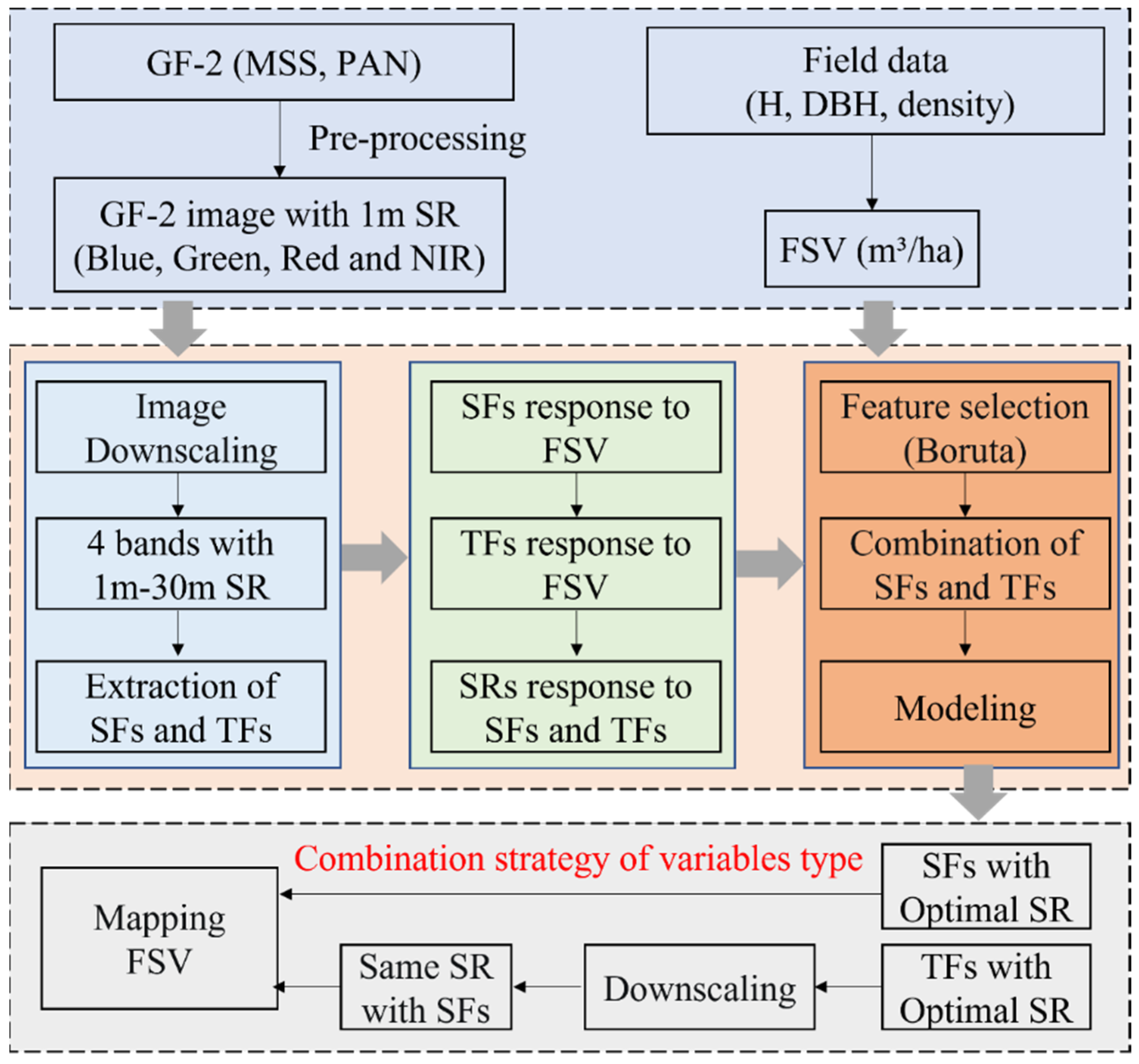
3. Material and Methods
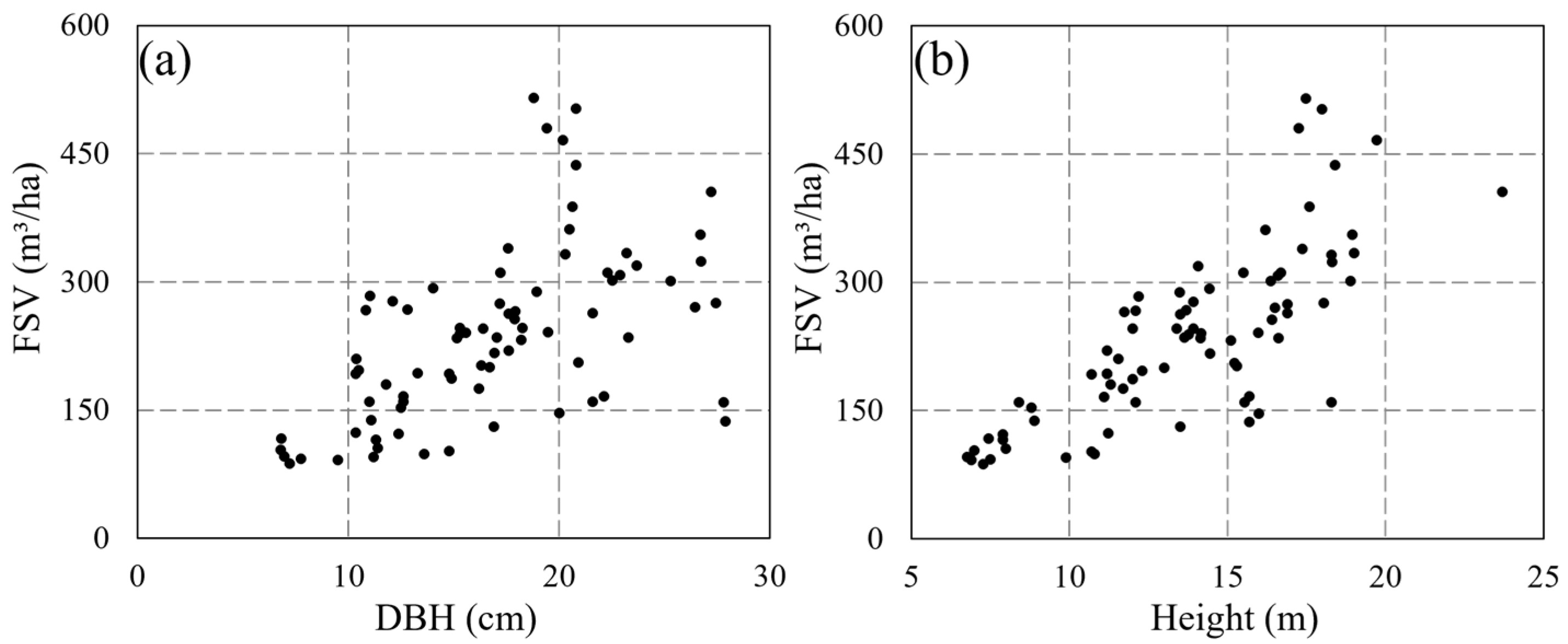
3.1. In Situ Data

To map the FSV of the study area, 79 ground samples (37 samples of larch and 42 samples of Chinese pine) were measured from September to October 2017, using stratified sampling according to stand age and spatial distribution. For each sample with a size of 25 m × 25 m, the positions of corners were precisely measured by GNSS with an error of less than 10 cm. Then, several parameters, such as diameter at breast height (DBH), tree height and crown diameter of each tree were measured. The wood volume of each tree was calculated according to the bivariate wood volume equation provided by Wangyedian Forestry, and the FSV of samples was obtained by the sum of the wood volumes of all trees in the plot. The FSV of the samples ranged from 87.44 to 514.96 m3/ha with a mean value of 235.86 m3/ha. The relationships of FSV, DBH and average height are shown in Figure 2.

3.2. Remote Sensing Data and Pre-Processing

In this study, meter-resolution images (GF-2) and medium-resolution images (Landsat 8 OLI and Sentinel-2) were acquired to map FSV based on the ground measurement date (Table 1). The GF-2 images include a panchromatic image with 0.81 m spatial resolution and four multispectral bands with 3.24 m spatial resolution (http://www.cresda.cn, accessed on 5 September 2017). Landsat 8 OLI includes six multispectral bands with 30 m (https://scihub.copernicus.eu/, accessed on 21 September 2017). Sentinel-2 images include four multispectral bands with 10 m and six bands with 20 m (https://scihub.copernicus.eu/, accessed on 22 September 2017). Additionally, DEM data with 30 m spatial resolution were also obtained for the topographic correction of optical satellite images (http://www.gscloud.cn/, accessed on 8 May 2019), and the topographic correction was accomplished using the SCS+C model in the ENVI 5.3 software.
Before extracting remote sensing features, all acquired images were pre-processed, including radiation correction, atmospheric correction, and topographic correction. For GF-2 images, one-meter multispectral images were obtained by fusing the multispectral bands and the panchromatic band, and the fused images were used to obtain down-scaled images with various spatial resolutions ranging from 1 to 30 m. The image downscaling is achieved using the “Resize data” module in ENVI 5.3 software, and the resampling method is the mean value method.

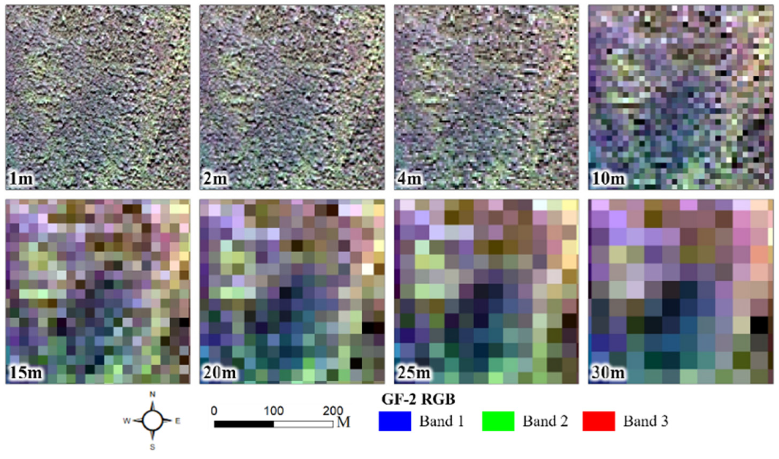
3.3. Down-Scaled Images with Various Spatial Resolutions

To reduce the errors induced by sensors and environmental factors, the method of down-scaling by averaging was employed to obtain images with various spatial resolutions based on fused GF-2 images with 1 m. To explore the relationships between FSV and the spatial resolutions of features (spectral and TF), the spatial resolutions of down-scaled images are 2 m, 4 m, 10 m, 15 m, 20 m, 25 m and 30 m (Figure 3). Figure 3 illustrated that the spatial information of the image gradually decreases with the decrease in spatial resolution.

3.4. Variable Extraction

Before mapping FSV, all alternative features should be extracted from acquired images. SF mainly conclude the spectral reflectance of various bands and vegetation indices. In this study, four fused multispectral bands with spatial resolutions ranging from 1 to 30 m were regarded as first type features, and various vegetation indices with various spatial resolutions were also extracted from four fused multispectral bands. For every spatial resolution image, nine common vegetation indices were extracted, including ratio vegetation index (RVI), enhanced vegetation index (EVI), normalized difference vegetation index (NDVI), difference vegetation index (DVI), red–green vegetation index (RGVI), atmospheric resistance vegetation index (ARVI), soil adjusted vegetation index (SAVI), modified soil adjusted vegetation index (MSAVI), and modified simple ratio (MSR). Additionally, the bands of Landsat 8 OLI and Sentinel-2 and their vegetation indices are also extracted from pre-processed images for mapping FSV in the next.
TF of images are indispensable variables to capture the surface features of forest canopy and can be used to improve the accuracy of mapping FSV [17,18,21,22]. In this study, the gray-scale spatial correlation matrix (GLCM) was employed to extract texture information with various sizes (3 × 3, 5 × 5, 7 × 7, 9 × 9), and eight TF of each size were obtained, including Variance (VAR), Entropy (EN), Data Range (DR), Homogeneity (HOM), Second Moment (SM), Dissimilarity (DIS), Contrast (CON) and Correlation (COR).

3.5. Combination Strategies of Variables with Various Spatial Resolutions

In general, all alternative features, spectral reflectance of various bands, vegetation indices and TF are extracted from multispectral optical images with the same spatial resolution. For images with high spatial resolution, the stability of spectral variables is decreased, which is caused by the heterogeneity of pixels. Furthermore, the richness of texture information largely depends on the spatial resolution of images. In other words, the sensitivity of spectral and TF in mapping FSV largely correlated with the spatial resolutions of images, and the optimal spatial resolutions are not synchronized for the two types of features. Therefore, the accuracy of mapping FSV using high spatial resolution images is not significantly higher than that from medium-resolution images [5,16]. To overcome the limitations of high-resolution images for mapping FSV, combination strategies of variables with various spatial resolutions were proposed to improve the accuracy of mapping FSV (Figure 4). The key to combination strategies is to find the optical spatial resolution of two types of variables in mapping FSV, respectively.
In complex forest environments, appropriate variable selection methods are necessary to reduce the effects of numerous surrogate variables and thus improve the predictive performance of the model. The Boruta algorithm is a fully correlated feature selection packing algorithm proposed by Kursa and Rudnicki in 2010 based on the random forest algorithm. The method compares the importance of the original attributes with the randomly obtained importance and gradually eliminates the irrelevant features to stabilize the test. In this study, all alternative spectral and TF were first extracted from each image at a specific spatial resolution (ranging from 1 to 30 m). Then, the optimal feature sets of spectral and TF were obtained by the Boruta algorithm, respectively [32]. The Boruta algorithm is implemented through the “Boruta” package from R studio 4.2.0.
In the next, three machine learning algorithms (random forest (RF), support vector machine (SVM) and K-nearest neighbor (KNN)) and multiple linear regression models were employed to estimate FSV using obtained optical feature sets of spectral and TF, respectively. Meanwhile, the coefficient of determination (R2), root means square error (RMSE), and relative RMSE (rRMSE) were calculated based on leave-one-out cross-validation to evaluate the performance of models. Finally, the optical spatial resolution of spectral and TF was derived from the smallest rRMSE values, respectively. Finally, for mapping the FSV of the study area, the TFs with the optimal spatial resolution are resampled to match the spatial resolution of SFs. In addition, to verify the contribution of the combination strategy applied in estimating FSV, predictions obtained from GF-2 were also compared with those obtained from Landsat 8 OLI and sentinel-2 images.

4. Results

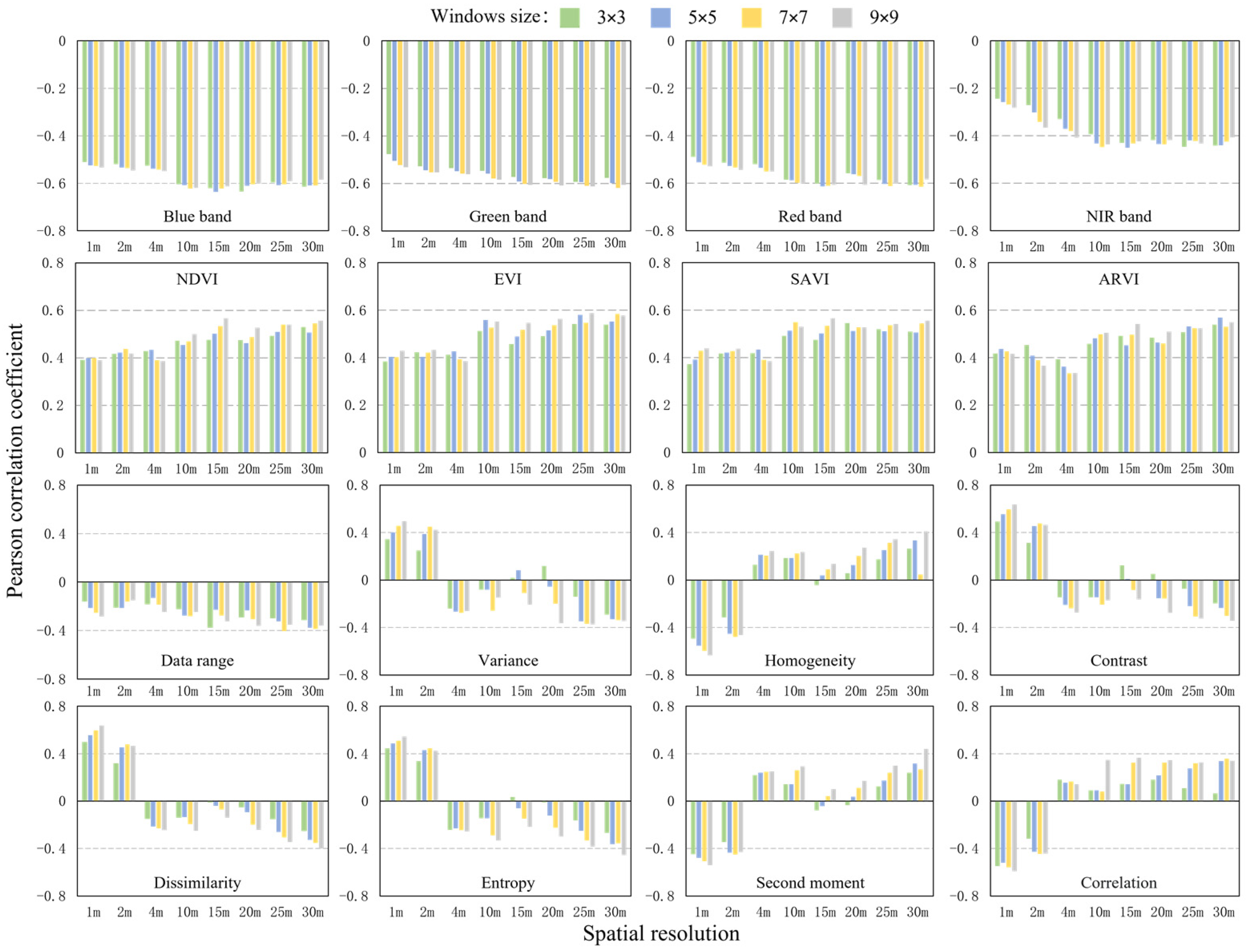
4.1. Sensitivity between Two Types of Features and Spatial Resolutions

To analyze the effect of spatial resolutions of two types of features (SFs and TFs), several down-scaling images with various spatial resolutions were obtained based on fused GF-2 images. Four statistical indicators, the maximum (MAX), minimum (MIN), mean and coefficient of variation (CV) of each band of down-scaling images, were employed to further demonstrate the spectral information varied with spatial resolutions in the planted forest (Figure 5). As the spatial resolution decreases, the coefficient of variation gradually decreases. It is also illustrated that the maximum and minimum values tend to mean values with decreased spatial resolutions in four bands. Based on the trends of statistical indicators, it is confirmed that the reduced spatial resolution of images leads to a reduced dispersion of the spectral values, but the average value of pixels remains the same. It can be inferred that the stability of SFs gradually increases as the spatial resolution decreases.
To further analyze the relationships between remote sensing variables and spatial resolutions, the autocorrelation of features (SFs and TFs) with different spatial resolutions was illustrated in Figure 6. The results showed that the autocorrelation coefficients were largely related to the spatial resolutions and types of features. For the SF (spectral reflectance of various bands and vegetation indices), autocorrelation coefficients decreased with the decrease in spatial resolution, and there are strong correlations between SF with different spatial resolutions. For the TF, correlations between TFs with different spatial resolutions are rather weak, and the results illustrated that the texture information has been greatly decreased with the decrease in spatial resolution. Especially, the autocorrelation between TF extracted from high spatial resolution images (1 m) is near zero. It is inferred that the information on SF does not lose greatly with the decrease in spatial resolutions, and the information on TF has a great loss with the decrease in spatial resolutions.
Furthermore, the Pearson correlation coefficients (PCCs) between partial variables and FSV were employed to explore the relationships between FSV and the spatial resolution of features (Figure 7). The results showed that the PCC between SFs and FSV gradually increases as the spatial resolution decreases, and these PCC were tending toward stability when the spatial resolution is larger than 10 m. On the contrary, the PCC between TFs and FSVs decreases and then increases with decreasing spatial resolution, and the highest PCC is obtained from TFs with 1 m spatial resolution. It is noteworthy that the sign of the correlation coefficient changes when the spatial resolution is reduced to 4 m (except for variables of data range). The results confirmed that spectral variables extracted from media spatial resolution images (larger than 10 m) have more sensitivity to FSV than those obtained from images with high spatial resolutions (less than 4 m), and texture variables are just the opposite.

4.2. Contributions of SFs and TFs in Mapping FSV

To verify the performance of SFs and TFs with different spatial resolutions in mapping FSV, all extracted features were combined into three variable sets: SFs, TFs and SFs+TFs. For each spatial resolution image, the optimal feature sets of each alternative variable set were obtained by the Boruta algorithm. Then, four regression algorithms, SVM, RF, KNN and MLR, were employed to construct the model between the variable sets and FSV. Figure 8 illustrated the results of accuracy indices (R2 and rRMSE) for mapping FSV using different variable sets. The results showed that the accuracy of mapped FSV improves with decreasing spatial resolution using spectral feature sets, and the accuracy indices tended to be stable using media spatial resolution features (ranging from 10 to 30 m). Using TFs, the accuracy indices largely related with spatial resolutions, and the best and the worst results were obtained from the variable sets with spatial resolution of 1 m and 15 m, respectively.
Furthermore, using variable sets combining SFs and TFs, the accuracy indices were obviously better than these results using a single spectral feature set or a single texture feature set. The results also proved that TFs have the capability to increase the accuracy of mapping FSV. On the other hand, the accuracy of the estimated FSV severely related to spatial resolutions using combining variable sets with the same spatial resolution, and the best results were obtained from combining the variable set with a spatial resolution of 15 m not from the images with a spatial resolution of 1 m. It is also illustrated that the optimal spatial resolutions of two types of features are not synchronized.
To further explore the capability of SFs and TFs in mapping FSV, scatter plots and residuals between predicted and measured FSV are illustrated in Figure 9. The results showed that underestimated and overestimated samples often occurred using a single SF or TF. Moreover, the results (Figure 8 and Figure 9) are proved that the combination variables set of SFs and TFs can effectively improve the accuracy of mapped FSV. Using combining variable sets (SFs+TFs) with the same spatial resolution, the RMSEs ranged from 66.5 to 68.6 m3/ha, and the smallest RMSE was obtained from the combining variable set with a spatial resolution of 15 m. Although the combination of TFs and SFs can improve the performance of estimating FSV, the advantage of TF extracted from high-resolution images is not demonstrated in mapping FSV.

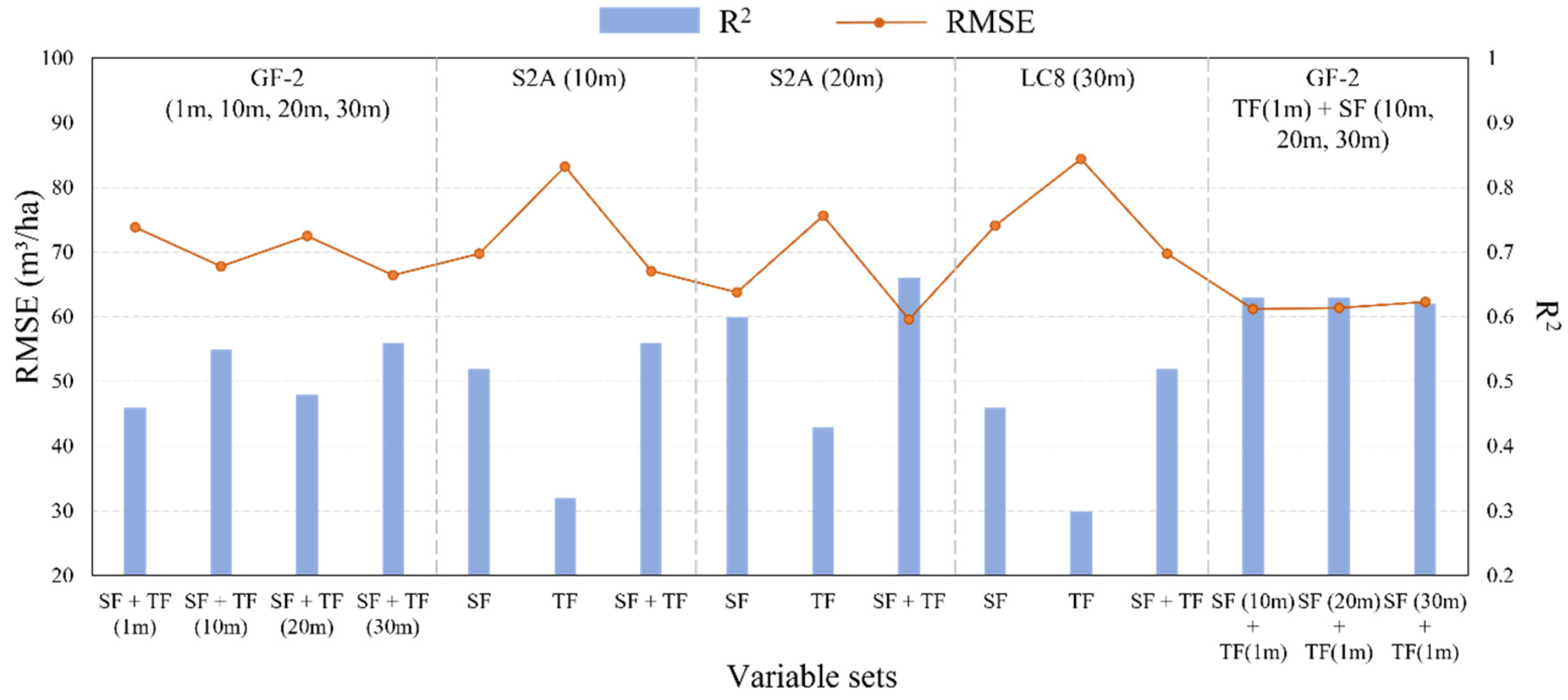
4.3. Combination Strategies of Variables with Various Spatial Resolutions

Previous results showed that the performance of SFs and TFs is highly dependent on the spatial resolution in estimating FSV, and the optimal spatial resolutions of the two types of features were different. To explore the advantages of high spatial resolution images for estimating FSV, a combined strategy of SFs and TFs with different spatial resolutions was constructed by obtaining optimal the spatial resolution of a single SF (SFs) and TF (TFs). Therefore, the combination sets of TFs and SFs with different spatial resolutions were proposed to map forest FSV. In our study, down-scale TFs (ranging from 2 to 30 m) were initially obtained from TFs extracted from fused images with a spatial resolution of 1 m. Then, combined sets were formed using SF and down-scaled TFs with the same spatial resolution. In addition, to compare the results of the combined strategy, SFs and TFs extracted from S2A and LC8 images with 10 m, 20 m and 30 m spatial resolution were also used to estimate FSV, and these results are listed in Table 2.
For estimating FSV using combined sets of SFs and TFs with the same spatial resolution, the variables set extracted from the Sentinel-2 images with 20 m spatial resolution (R2 ranged from 0.60 to 0.66, rRMSE ranged from 25.01% to 27.00%) was significantly better than other variable sets from GF-2 and Landsat-8 images. Using variable sets with the same spatial resolutions, it is inferred that the accuracy of mapped FSV is largely related to spatial resolutions and optical remote sensing images with medium spatial resolutions (10~30 m) are more suitable than other images with high spatial resolutions (1~4 m). However, the capability of TF extracted from high-resolution images cannot be demonstrated in mapping forest FSV.
After using combination strategies of variables with various spatial resolutions, the rRMSE and R2 of three combining strategies ranged from 24.66% to 28.55% and from 0.55 to 0.67, respectively. The optimal result (rRMSE = 24.66%, and R2 = 0.67) was obtained from a variable set (GF-2 (SF (30 m) + TF (1 m))) using the SVM model. It is demonstrated that the accuracy of mapped FSV using proposed combination strategies is obviously higher than results derived from GF-2, Sentinel-2 and Landsat-8 images with the same spatial resolutions of variable sets. It is also proved that TFs derived from high spatial resolutions have great potential to improve the accuracy of mapping FSV, and the contribution of these valuable TF depended on the approaches of extracting and using strategies.
To further clarify the contribution of TF extracted from high spatial resolutions, scatter plots of the optimal results from three combined strategies, Sentinel-2 and Landsat-8 images are shown in Figure 10. The proposed combined strategies reduced the errors caused by the overestimation and underestimation, and the results were even slightly higher than these results obtained from variable sets (Sentinel-2 (SF+TF, 20 m)), which are derived from Sentinel-2 images with 13 multispectral bands. Using Sentinel-2 and Landsat-8 images, the main factor affecting accuracy is underestimated samples with high forest, which is caused by the optical saturation phenomenon. The results also showed that the predicted samples with high FSV have been improved using the proposed combined strategies, and the accuracy of estimated forest FSV has naturally improved. It is inferred that TFs extracted from high spatial resolutions have the capability to delay the optical saturation levels. The advantage of TFs extracted from high-resolution images is obviously demonstrated in mapping FSV by using combination strategies of variables with various spatial resolutions. Finally, the spatial distribution of FSV in Wangyedian Forestry is shown in Figure 11. FSV in coniferous forests is concentrated in the central and northeastern areas, and there is lower FSV in the west and southeast.

5. Discussion

5.1. Effect of Spatial Resolution on SFs and TFs

By naturally reflecting the growth status of the forest, SFs are reported to be closely related to canopies and leaf structure parameters [6,7,8,15,16]. Furthermore, the sensitivity between SFs and forest FSV is also affected by the spatial resolutions of images. In this study (Figure 5 and Figure 6), Pearson correlation coefficients between SFs and forest FSV increased with the decreased spatial resolutions of images and tend to be stable when the spatial resolution is larger than 10 m. The main reasons are that the number of sub-components in pixels depends on the spatial resolutions of images. For high spatial resolution images, a pixel may contain only one scene component, so the instability and low Pearson correlation coefficients of extracted SFs were observed caused by strong randomness and uncertainty between pixels. In contrast, as the spatial resolution of images is reduced to larger than 10 m, a pixel is more likely to be composed of multiple scene components, which implies a smaller range and coefficient of variation of pixel values within the scene. Therefore, it is inferred that SFs extracted from the images with medium spatial resolutions are more suitable to apply in mapping forest FSV. Although the correlation between FSV and SFs extracted from optical images can be improved by decreasing the spatial resolutions, overestimated and underestimated results are still inevitable in mapping forest FSV.
Furthermore, TFs are also commonly extracted from optical images with different spatial resolutions. It is reported that TFs are related to the spatial distribution of sub-components (light canopy, shadow canopy, light background, and shadow background) in the scene [20,33,34,35]. The images with different spatial resolutions contain different information about the four scene components in a single pixel, resulting in large differences in the distribution of pixels in the image. Therefore, the richness of TF and their sensitivity to FSV largely depend on the spatial resolution of images [23]. Previous studies also indicated that the spatial resolution of optical images severely affects the quality of TF and the performance of employed models in complex forests [18,21,36,37]. In our study, TF with different sizes (3 × 3, 5 × 5, 7 × 7, 9 × 9) were extracted from down-scaled images with spatial resolutions ranging from 1 to 30 m. The results demonstrated that the correlation between TFs and FSV decreased first and then increased with the decrease in spatial resolution and the highest correlation is obtained from images with 1 m spatial resolution, and similar results were also obtained in previous studies [23,38].
Additionally, it is proved that TFs derived from GF-2 images have great potential to improve the accuracy of mapping FSV, and the contribution of features depends on the approaches of extracting and combination strategies. Figure 7 and Figure 8 also clearly illustrated that the optimal spatial resolutions of two types of features are not synchronized. Therefore, the accuracy of mapping FSV using features with the same resolution extracted from GF-2 images is significantly lower than that from Sentinel-2 and Landsat-8 images. The advantages of high spatial resolution images are not well represented in mapping forest FSV. It is necessary to select an appropriate method to combine features of different spatial resolutions.

5.2. Contribution of the Combination of SFs and TFs in Mapping FSV

It has been reported that underestimated FSV are often obtained by common methods using SF by capturing the horizontal information of forest canopies [5,6,18,21,39,40]. The TFs have been proven to be capable of improving the underestimated results caused by spectral saturation [5,6,18,21,23]. In our study, combining variable sets (SFs+TFs) extracted from different images were obtained and the accuracy indices of mapped FSV are illustrated in Figure 12. It is found that the contributions of combining variable sets (SFs+TFs) are obviously higher than single SFs or single TFs in mapping forest FSV. The results also demonstrate that rRMSE values derived from GF-2 images are significantly larger than other results derived from S2A (10 m), S2A (20 m) and LC8 (30 m) using combining variable set (SFs+TFs) with the same spatial resolution. After using combination strategies of variables with various spatial resolutions, the accuracy of results is obviously improved, and the advantage of TF extracted from high-resolution images is demonstrated in mapping FSV.
Furthermore, the spectral saturation problem of optical images is still a great challenge in mapping forest FSV [11,16,41,42]. Generally, the spectral saturation problem is caused by different reasons, and optical remote sensing images have been criticized for their inability to pass through a dense tree canopy [5,6,18,21,23]. When the forest canopy is closed, the height of the trees can continue to grow, and the FSV continues to increase without changing the spectral reflectance of the canopy. Therefore, how to mitigate the saturation problem of optical images has become a research hotspot. Since the physical characteristics of different tree species vary greatly, solutions for spectral saturation are to extract seasonal variation information of the canopy using multi-temporal optical images [38,42]. It was shown that extracting canopy growth information using optical data across growing seasons can improve both underestimation and overestimation in fast-growing tree species (e.g., eucalyptus) [42]. Zhu et al. also showed that the phenological information contained in the NDVI time-series could improve the accuracy of AGB estimation, especially for areas with large AGB [43].
Recently, widely used TFs extracted from optical images have also proved effective in alleviating the spectral saturation problem [18,21,23]. In this study, the combined variables of TFs and SFs significantly improved the underestimation of FSV, demonstrating the contribution of TFs to mitigate the saturation problem (Figure 8 and Figure 9). Especially, combination strategies of variables with various spatial resolutions are proposed to improve the accuracy of mapping forest FSV using a high spatial resolution of images (GF-2). However, detailed information on canopy structure is difficult to obtain from images with a medium spatial resolution (e.g., Sentinel 2 and Landsat 8 OLI) [29,44,45,46,47]. Therefore, TFs extracted from images with medium spatial resolution have great limitations when it comes to improving the accuracy of mapping FSV.

6. Conclusions

In this study, a new combination strategy of variables was developed with various spatial resolutions derived from GF-2 images to map forest FSV. The results show that the sensitivity between FSV and features is highly related to the spatial resolutions of images. It is also confirmed that the optimal spatial resolutions of two types of features are not synchronized, and the advantages of high spatial resolution images (GF-2) are not well represented in mapping forest FSV. After using the proposed combination strategy of variables with various spatial resolutions, the results demonstrate that the accuracy of mapped FSV using the proposed combination strategies is significantly higher than these results derived from GF-2, Sentinel-2 and Landsat-8 images with the same spatial resolutions of variable sets. The optimal result was obtained from the variable set (GF-2 (SF (30 m) + TF (1 m))) using the SVM model. It is concluded that TF derived from GF-2 images have great potential to improve the accuracy of mapping FSV, and the advantage of TF extracted from high-resolution images depends on the approaches of extracting and combination strategies.

Author Contributions

Conceptualization, Z.L. and J.L.; methodology, Z.L. and J.L.; software, X.X., H.L. (Hao Liu) and T.Z.; validation, Z.L., H.L. (Hao Liu) and X.X.; formal analysis, Z.L and X.X.; investigation, Z.L., P.Y., Z.Y., H.L. (Hao Liu), X.X. and T.Z.; resources, H.L. (Hui Lin) and J.L.; data curation, Z.L. and X.X.; writing—original draft preparation, Z.L. and J.L.; writing—review and editing, Z.L. and J.L.; visualization, Z.L. and H.L.; supervision, J.L. and H.L. (Hui Lin); project administration, H.L. (Hui Lin) and J.L.; funding acquisition, H.L. (Hui Lin) and J.L. All authors have read and agreed to the published version of the manuscript.

Funding

This research was funded by the Hunan Provincial Natural Science Foundation of China (Project number: 2021JJ31158); the Excellent Youth Project of the Scientific Research Foundation of the Hunan Provincial Department of Education (Project number: 21B0246); supported by the National Natural Science Foundation of China (Project number: 32171784) and the National Key R&D Program of China project “Key Technologies for Monitoring Forest Plantation Resources” (Project number: 2017YFD0600900).

Data Availability Statement

The observed GSV data from the sample plots and the spatial distribution data of forest resources presented in this study are available on request from the corresponding author. Those data are not publicly available due to privacy and confidentiality reasons. The GF-2 images are available from China Centre for Resources Satellite Data and Application website at http://www.cresda.com/CN/ (accessed on 10 May 2020).

Conflicts of Interest

The authors declare no conflict of interest.

References

  1. Seidl, R.; Spies, T.A.; Peterson, D.L.; Stephens, S.L.; Hicke, J.A. Searching for resilience: Addressing the impacts of changing disturbance regimes on forest ecosystem services. J. Appl. Ecol. 2016, 53, 120–129. [Google Scholar] [CrossRef] [Green Version]
  2. Schimel, D.S. Terrestrial ecosystem and carbon cycle. Glob. Chang. Biol. 2006, 1, 77–91. [Google Scholar] [CrossRef]
  3. Toan, T.L.; Quegan, S.; Davidson, M.; Balzter, H.; Ulander, L. The biomass mission: Mapping global forest biomass to better understand the terrestrial carbon cycle. Remote Sens. Environ. 2011, 115, 2850–2860. [Google Scholar] [CrossRef] [Green Version]
  4. Long, J. A Combined Strategy of Improved Variable Selection and Ensemble Algorithm to Map the Growing Stem Volume of Planted Coniferous Forest. Remote Sens. 2021, 13, 4631. [Google Scholar]
  5. Li, X.; Liu, Z.; Wang, G.; Long, J.; Zhang, M. Estimating the Growing Stem Volume of Chinese Pine and Larch Plantations based on Fused Optical Data Using an Improved Variable Screening Method and Stacking Algorithm. Remote Sens. 2020, 12, 871. [Google Scholar] [CrossRef] [Green Version]
  6. Jiang, F.; Kutia, M.; Sarkissian, A.J.; Lin, H.; Wang, G. Estimating the Growing Stem Volume of Coniferous Plantations Based on Random Forest Using an Optimized Variable Selection Method. Sensors 2020, 20, 7248. [Google Scholar] [CrossRef]
  7. Long, J.; Lin, H.; Wang, G.; Sun, H.; Yan, E. Estimating the Growing Stem Volume of the Planted Forest Using the General Linear Model and Time Series Quad-Polarimetric SAR Images. Sensors 2020, 20, 3957. [Google Scholar] [CrossRef]
  8. Jiang, F.; Kutia, M.; Ma, K.; Chen, S.; Long, J.; Sun, H. Estimating the aboveground biomass of coniferous forest in Northeast China using spectral variables, land surface temperature and soil moisture. Sci. Total Environ. 2021, 785, 147335. [Google Scholar] [CrossRef] [PubMed]
  9. Fassnacht, F.; Hartig, F.; Latifi, H.; Berger, C.; Hernández, J.; Corvalán, P.; Koch, B. Importance of sample size, data type and prediction method for remote sensing-based estimations of aboveground forest biomass. Remote Sens. Environ. 2014, 154, 102–114. [Google Scholar] [CrossRef]
  10. Lu, D. The potential and challenge of remote sensing-based biomass estimation. Int. J. Remote Sens. 2006, 27, 1297–1328. [Google Scholar] [CrossRef]
  11. Reis, A.; Franklin, S.; Mello, J.; Junior, F. Volume estimation in a Eucalyptus plantation using multi-source remote sensing and digital terrain data: A case study in Minas Gerais State, Brazil. Int. J. Remote Sens. 2019, 40, 2683–2702. [Google Scholar] [CrossRef]
  12. Sinha, S.; Jeganathan, C.; Sharma, L.K.; Nathawat, M.S. A review of radar remote sensing for biomass estimation. Int. J. Environ. Sci. Technol. 2015, 12, 1779–1792. [Google Scholar] [CrossRef] [Green Version]
  13. Zheng, S.; Cao, C.; Dang, Y.; Xiang, H.; Zhao, J.; Zhang, Y. Retrieval of forest growing stock volume by two different methods using Landsat TM images. Int. J. Remote Sens. 2014, 35, 29–43. [Google Scholar] [CrossRef]
  14. Urbazaev, M.; Thiel, C.; Migliavacca, M.; Reichstein, M.; Rodriguez, P.; Schmullius, C. Improved Multi-Sensor Satellite-Based Aboveground Biomass Estimation by Selecting Temporally Stable Forest Inventory Plots Using NDVI Time Series. Forests 2016, 7, 169. [Google Scholar] [CrossRef]
  15. Sergio, M.; Camarero, J.; José, M.; Natalia, M.; Marina, P.; Miquel, T.; Antonio, G.; Cesar, A.; Upasana, B.; Ahmed, E. Diverse relationships between forest growth and the Normalized Difference Vegetation Index at a global scale. Remote Sens. Environ. 2016, 187, 14–29. [Google Scholar] [CrossRef] [Green Version]
  16. Li, X.; Lin, H.; Long, J.; Xu, X. Mapping the Growing Stem Volume of the Coniferous Plantations in North China Using Multispectral Data from Integrated GF-2 and Sentinel-2 Images and an Optimized Feature Variable Selection Method. Remote Sens. 2021, 13, 2740. [Google Scholar] [CrossRef]
  17. Astola, M. Comparison of Sentinel-2 and Landsat 8 imagery for forest variable prediction in boreal region. Remote Sens. Environ. 2019, 223, 257–273. [Google Scholar] [CrossRef]
  18. Lu, D.; Chen, Q.; Wang, G.; Moran, E.; Saah, D. Aboveground Forest Biomass Estimation with Landsat and LiDAR Data and Uncertainty Analysis of the Estimates. Int. J. For. Res. 2012, 2012, 1–16. [Google Scholar] [CrossRef] [Green Version]
  19. Chrysafis, I.; Mallinis, G.; Siachalou, S.; Patias, P. Assessing the relationships between growing stock volume and Sentinel-2 imagery in a Mediterranean forest ecosystem. Remote Sens. Lett. 2017, 8, 508–517. [Google Scholar] [CrossRef]
  20. Yang, C.; Huang, H.E.; Wang, S. Estimation of tropical forest biomass using Landsat TM imagery and permanent plot data in Xishuangbanna, China. Int. J. Remote Sens. 2011, 32, 5741–5756. [Google Scholar] [CrossRef]
  21. Lu, D.; Chen, Q.; Wang, G.; Liu, L.; Li, G.; Moran, E. A survey of remote sensing-based aboveground biomass estimation methods in forest ecosystems. Int. J. Digit. Earth 2014, 9, 63–105. [Google Scholar] [CrossRef]
  22. Li, G.; Xie, Z.; Jiang, X.; Lu, D.; Chen, E. Integration of ZiYuan-3 Multispectral and Stereo Data for Modeling Aboveground Biomass of Larch Plantations in North China. Remote Sens. 2019, 11, 2328. [Google Scholar] [CrossRef] [Green Version]
  23. Yue, J.; Yang, G.; Tian, Q.; Feng, H.; Xu, K.; Zhou, C. Estimate of winter-wheat above-ground biomass based on UAV ultrahigh-ground-resolution image textures and vegetation indices. ISPRS J. Photogramm. Remote Sens. 2019, 150, 226–244. [Google Scholar] [CrossRef]
  24. Sarker, M.; Nichol, J.; Ahmad, B.; Busu, I.; Rahman, A. Potential of Texture Measurements of Two-date Dual Polarization PALSAR Data for the Improvement of Forest Biomass Estimation. ISPRS J. Photogramm. Remote Sens. 2012, 69, 146–166. [Google Scholar] [CrossRef]
  25. Lu, D.; Moran, E.; Batistella, M. Linear Mixture Model Applied to Amazonian Vegetation Classification. Remote Sens. Environ. 2003, 87, 456–469. [Google Scholar] [CrossRef] [Green Version]
  26. Song, C.; Dickinson, M.B.; Su, L.; Su, Z.; Yaussey, D. Estimating average tree crown size using spatial information from Ikonos and QuickBird images: Across-sensor and across-site comparisons. Remote Sens. Environ. 2010, 114, 1099–1107. [Google Scholar] [CrossRef]
  27. Pouliot, D.; King, D.; Bell, F.; Pitt, D. Automated tree crown detection and delineation in high-resolution digital camera imagery of coniferous forest regeneration. Remote Sens. Environ. 2002, 82, 322–334. [Google Scholar] [CrossRef]
  28. Sakar, T.; Anssi, P. Performance of different spectral and textural aerial photograph features in multi-source forest inventory. Remote Sens. Environ. 2005, 94, 256–268. [Google Scholar] [CrossRef]
  29. Song, C.; Woodcock, C.E. The spatial manifestation of forest succession in optical imagery: The potential of multiresolution imagery. Remote Sensing Environ. 2002, 82, 271–284. [Google Scholar] [CrossRef]
  30. Leckie, D.; Walsworth, N.; Gougeon, F. Identifying tree crown delineation shapes and need for remediation on high resolution imagery using an evidence-based approach. ISPRS J. Photogramm. Remote Sens. 2016, 114, 206–227. [Google Scholar] [CrossRef]
  31. Leckie, D.; Gougeon, F.A.; Walsworth, N.; Paradine, D. Stand delineation and composition estimation using semi-automated individual tree crown analysis. Remote Sens. Environ. 2003, 85, 355–369. [Google Scholar] [CrossRef]
  32. Zhao, Q.; Yu, S.; Zhao, F.; Tian, L.; Zhao, Z. Comparison of machine learning algorithms for forest parameter estimations and application for forest quality assessments. For. Ecol. Manag. 2019, 434, 224–234. [Google Scholar] [CrossRef]
  33. Haralick, R. Textural features for image classification. IEEE Trans. Syst. Man Cybern. 1973, 3, 610–621. [Google Scholar] [CrossRef] [Green Version]
  34. Yang, P.; Hou, Z.; Liu, X.; Shi, Z. Texture feature extraction of mountain economic forest using high spatial resolution remote sensing images. In Proceedings of the 2016 IEEE International Geoscience and Remote Sensing Symposium (IGARSS), Beijing, China, 10–15 July 2016. [Google Scholar]
  35. Ruiz, L.; Inan, I.; Baridon, J.; Lanfranco, J. Combining multispectral images and selected textural features from high resolution images to improve discrimination of forest canopies. In Proceedings of the Image and Signal Processing for Remote Sensing IV, Barcelona, Spain, 21–25 September 1998; Volume 3500, pp. 124–134. [Google Scholar]
  36. Gao, T.; Zhu, J.; Zheng, X.; Shang, G.; Huang, L.; Wu, S. Mapping Spatial Distribution of Larch Plantations from Multi-Seasonal Landsat-8 OLI Imagery and Multi-Scale Textures Using Random Forests. Remote Sens. 2015, 7, 1702–1720. [Google Scholar] [CrossRef] [Green Version]
  37. Wood, E.; Pidgeon, A.; Radeloff, V.; Keuler, N. Image texture as a remotely sensed measure of vegetation structure. Remote Sens. Environ. 2012, 121, 516–526. [Google Scholar] [CrossRef]
  38. Powell, S.L.; Cohen, W.B.; Healey, S.P.; Kennedy, R.E.; Moisen, G.G.; Pierce, K.B.; Ohmann, J.L. Quantification of live aboveground forest biomass dynamics with Landsat time-series and field inventory data: A comparison of empirical modeling approaches. Remote Sens. Environ. 2010, 114, 1053–1068. [Google Scholar] [CrossRef]
  39. Dube, T.; Sibanda, M.; Shoko, C.; Mutanga, O. Stand-volume estimation from multi-source data for coppiced and high forest Eucalyptus spp. silvicultural systems in KwaZulu-Natal, South Africa. ISPRS J. Photogramm. 2017, 132, 162–169. [Google Scholar] [CrossRef]
  40. Moudrý, V.; Gdulová, K.; Fogl, M.; Klápště, P.; Urban, R.; Komárek, J.; Moudrá, L.; Štroner, M.; Barták, V.; Solský, M. Comparison of leaf-off and leaf-on combined UAV imagery and airborne LiDAR for assessment of a post-mining site terrain and vegetation structure: Prospects for monitoring hazards and restoration success. Appl. Geogr. 2019, 104, 32–41. [Google Scholar] [CrossRef]
  41. Ghosh, S.M.; Behera, M.D.; Jagadish, B.; Das, A.K.; Mishra, D.R. A novel approach for estimation of aboveground biomass of a carbon-rich mangrove site in India. J. Environ. Manag. 2021, 292, 112816. [Google Scholar] [CrossRef]
  42. Liu, Z.; Ye, Z.; Xu, X.; Lin, H.; Zhang, T.; Long, J. Mapping Forest Stock Volume Based on Growth Characteristics of Crown Using Multi-Temporal Landsat 8 OLI and ZY-3 Stereo Images in Planted Eucalyptus Forest. Remote Sens. 2022, 14, 5082. [Google Scholar] [CrossRef]
  43. Zhu, X.; Liu, D. Improving Forest aboveground biomass estimation using seasonal Landsat NDVI time-series. ISPRS J. Photogramm. Remote Sens. 2015, 102, 222–231. [Google Scholar] [CrossRef]
  44. Ke, Y.; Quackenbush, L. A review of methods for automatic individual tree-crown detection and delineation from passive remote sensing. Int. J. Remote Sens. 2011, 32, 4725–4747. [Google Scholar] [CrossRef]
  45. Ke, Q.; Quackenbush, L. A comparison of three methods for automatic tree crown detection and delineation from high spatial resolution imagery. Int. J. Remote Sens. 2011, 32, 3625–3647. [Google Scholar] [CrossRef]
  46. Gougeon, F.; Leckie, D. The individual tree crown approach applied to Ikonos images of a coniferous plantation area. Photogramm Eng. Remote Sens. 2006, 72, 1287–1297. [Google Scholar] [CrossRef]
  47. Gougeon Francois, A.; Leckie Donald, G. Forest information extraction from high spatial resolution images using an individual tree crown approach. Quintessence 2003, 34, 749–760. [Google Scholar] [CrossRef] [Green Version]
Figure 1. Location of the study area and the map of ground measured samples.
Forests 14 01175 g001
Figure 2. The relationships between DBH, average height and FSV: (a) is the relationship between FSV and DBH, and (b) is the relationship between FSV and average height.
Forests 14 01175 g002
Figure 3. Down-sampled images with various spatial resolutions based on fused GF-2 images.
Forests 14 01175 g003
Figure 4. Flowchart of experiment methodology.
Forests 14 01175 g004
Figure 5. Statistics results of each band with various spatial resolutions.
Forests 14 01175 g005
Figure 6. Pearson correlation coefficients between spectral and TF with various resolutions (TFs are extracted from the blue band of GF-2, filter size: 9 × 9).
Forests 14 01175 g006
Figure 7. The Pearson correlation coefficients between features and FSV (TFs are from the blue band of GF-2).
Forests 14 01175 g007
Figure 8. The accuracy of mapped FSV using four models with different variable sets and spatial resolutions.
Forests 14 01175 g008
Figure 9. Scatter plot of estimated and measured FSV.
Forests 14 01175 g009
Figure 10. Scatter plot of estimated vs. measured FSV (GF-2, S2A and LC8).
Forests 14 01175 g010
Figure 11. Spatial distribution of FSV, (a) is from the combination of SFs with 10 m spatial resolution and TFs with 1 m spatial resolution, (b) is from the combination of SFs with 20 m spatial resolution and TFs with 1 m spatial resolution and (c) is from the combination of SFs with 30 m spatial resolution and TFs with 1 m spatial resolution, (df) are from S2A with 10 m and 20 m spatial resolution and LC8 with 30 m spatial resolution, respectively.
Forests 14 01175 g011
Figure 12. The results of FSV were estimated using RF models and variable sets from different data sources.
Forests 14 01175 g012
Table 1. Information on three types of remote sensing images.
SensorsSpatial Resolution (m)BandsNumber of BandsAcquisition Data
GF-21Pan15 September 2017
4Blue, Green, Red and NIR4
Sentinel-210Blue, Green, Red and NIR422 September 2017
20Red Edge 1–4, SWIR 1, 26
Landsat 830Blue, Green, Red, NIR, SWIR 1, 2621 September 2017
Table 2. The results of mapping forest FSV using GF-2, Sentinel-2 and Landsat-8 images using combined sets with various spatial resolutions.
Variable SetsRFSVMKNNMLR
RMSE (m3/ha)rRMSE (%)R2RMSE (m3/ha)rRMSE (%)R2RMSE (m3/ha)rRMSE (%)R2RMSE (m3/ha)rRMSE (%)R2
GF-2 (SF+TF, 1 m)73.8731.320.4667.4730.300.5272.6030.780.4873.1931.150.47
GF-2 (SF+TF, 10 m)67.7928.740.5565.9927.980.5765.1727.630.5879.2033.580.38
GF-2 (SF+TF, 20 m)72.4830.730.4868.5629.070.5473.4931.160.4775.1631.870.44
GF-2 (SF+TF, 30 m)66.4528.180.5669.7929.590.5271.0630.130.5074.6031.630.45
Sentinel-2 (SF+TF, 10 m)67.1028.450.5666.5528.220.5665.8027.900.5779.8433.850.37
Sentinel-2 (SF+TF, 20 m)59.6125.010.6662.7626.610.6163.6727.000.6062.3826.450.62
Landsat-8 (SF+TF, 30 m)69.7929.590.5271.7830.430.4973.5931.200.4781.1534.410.35
GF-2 (SF (10 m) + TF (1 m))61.2125.950.6358.4824.800.6658.1324.650.6665.5627.800.58
GF-2 (SF (20 m) + TF (1 m))61.3826.030.6361.2125.950.6360.0425.460.6467.3328.550.55
GF-2 (SF (30 m) + TF (1 m))62.3026.410.6258.1624.660.6760.3925.610.6464.5327.360.59
Disclaimer/Publisher’s Note: The statements, opinions and data contained in all publications are solely those of the individual author(s) and contributor(s) and not of MDPI and/or the editor(s). MDPI and/or the editor(s) disclaim responsibility for any injury to people or property resulting from any ideas, methods, instructions or products referred to in the content.

