Article

Conditional Performance Evaluation: Using Wildfire Observations for Systematic Fire Simulator Development

1
School of Ecosystem and Forest Sciences, Faculty of Science, University of Melbourne, Burnley 3121, Australia
2
School of Ecosystem and Forest Sciences, University of Melbourne, Creswick 3363, Australia
3
School of Ecosystem and Forest Sciences, University of Melbourne, Parkville 3052, Australia
*
Author to whom correspondence should be addressed.
Forests 2018, 9(4), 189; https://doi.org/10.3390/f9040189
Submission received: 2 February 2018 / Revised: 26 March 2018 / Accepted: 2 April 2018 / Published: 6 April 2018

Abstract

:
Faster than real-time wildland fire simulators are being increasingly adopted by land managers to provide decision support for tactical wildfire management and assist with strategic risk planning. These simulators are typically based on simple forward rate-of-spread algorithms that were predominantly developed using observations of experimental fires. Given their operational use, it is important that fire simulators be assessed in terms of their performance for their intended use; predicting the spatial progression of wildfires. However, the conditions under which wildfires occur cannot be easily replicated experimentally. We describe and demonstrate a method for use in model development, whereby a dataset comprised of wildfire case-studies is used for evaluating the predictive performance of fire simulators. Two different versions of the model PHOENIX RapidFire were assessed, one incorporating a novel algorithm that accounts fine-scale spatial variation in landscape dryness. Evaluation was done by comparing simulator predictions against contemporaneous observations of 9 different wildfires that occurred in Australia. Performance was quantified using the sum of the Area Difference Indices—a measure of prediction overlap calculated for each prediction/observation pair. The two versions of the model performed similarly, with the newer version being marginally (but not statistically significantly) better when outcomes were summarised across all fires. Despite this, it did not perform better in all cases, with three of the 9 fires better predicted using the original model. Wildfire evaluation datasets were demonstrated to provide valuable feedback for model development, however the limited availability of data means power is lacking for detailed comparisons. With increasingly extreme weather conditions resulting from climate change, conditions under which wildfires occur are likely to continue to extend well beyond those under which fire models algorithms were developed. Consequently, the adoption of improved methods for collecting and utilising wildfire data is critical to ensure fire simulators retain relevance.

Graphical Abstract

1. Introduction

Wildfires occur in parts of the world where there is a suitable combination of ignition sources, productivity and aridity [1,2]. Where they occur, they have the potential to impact human values. Impacts can include the loss of lives, damage to infrastructure and disruptions to ecosystem services [3]. Where wildfires occur in populated areas, land managers—typically governments—commonly enact measures to prepare, respond and recover from them [4]. The need to anticipate potential fire behaviour and its resultant impacts has led to the development of the field of fire modelling. Fire modelling has a long history, beginning early in the 20th century, driven by an aim to use available information to predict fire behaviour to support management activities. Early models were predominantly designed to predict the forward rate of spread (FROS) of the fastest moving windward part of fires based on inputs of fuel, weather and topography. This is used to create forecasts of likely fire progression during fires and provide generalised indications of fire danger [5,6]. More recently, taking advantage of increasing computing power and data availability, FROS models have been extended into fire simulators; models that simulate the propagation of fires through space and time, enabling maps of progression to be produced. For this study, we use the definition of fire simulators sensu Sullivan [7], to represent empirical or quasi-empirical faster-than-real-time models intended for use at large scales. Other forms of fire simulation exist, such those that emulate physical processes, however they are not considered here [8].
Fire simulators have been adopted operationally by fire management agencies in different countries, including FARSITE [9] in the United States and Europe, PHOENIX RapidFire (PHOENIX) [10] in Australia, and Prometheus [11] in Canada and New Zealand. The fire progression maps that they produce provide an indication of the areas of the landscape likely to be impacted and indicative times at which these impacts may occur. This information is used to devise fire suppression strategies and inform the issuing of warnings and planning of evacuations. Additionally, by simulating hypothetical fires, they are being used to provide spatially explicit estimates of wildfire risk throughout the landscape [12,13,14,15]. Such approaches can be used to identify key areas in which to prioritise management intervention [16] or allow alternative management strategies to be compared in terms of risk reduction efficacy [17]. Given their active use in decision making, it is important that the performance and limitations of the various fire simulators available be understood [18,19]. This is particularly the case when looking to improve, compare or calibrate models, as there must be some objective basis from which to evaluate change in performance.
The FROS algorithms that form the basis of fire simulators have typically been calibrated or entirely empirically fit to observations of experimental fires [20]. As FROS models produce point rates of spread, their performance is relatively straightforward to evaluate by using observations drawn from wildfires: predictions can be compared with corresponding observations of fireline positions between two points in time [21,22,23]. A limitation with experimental fires is they must be implemented in a safe manner; this means they cannot be undertaken under conditions that are likely to result in uncontrollable wildfires. While some models do incorporate wildfire observations for evaluation [24,25,26], the majority of data is typically from lower intensity fires. Consequently, wildfire conditions are typically beyond the model development range [25], although there is some evidence that FROS models can provide a reasonable result when extrapolating to wildfire conditions [27].
When creating a fire simulator from a FROS algorithm, there are a number of additional properties to consider [28]. In particular, a fire simulator must account for progression through space and time. In doing this, it must consider (amongst other things) heterogeneous vegetation fuels [29,30], backing and flanking fire behaviour, the effects of changing weather, variation in fine fuel moisture [31], the influence of topography [32] and the effect of interactions between these factors [33,34]. Consequently, the development of a fire simulator from a FROS algorithm requires a large number of assumptions that were not tested in the initial algorithm development process. Such assumptions should be verified for the conditions of use if the models are to be relied upon. Compounding the challenge for spatialising fire prediction is the occurrence of emergent extreme fire behaviours that are localised phenomena that can affect fire progression, including fire tornados, crown fires and mass spotting events [33,35,36,37,38,39,40]. Fires are an inherently spatial event, so it is unrealistic to expect that fire simulators can be robust if they are solely derived from FROS models without additional testing. To allow the further development of simulation models, spatially explicit methods of performance evaluation are necessary where predictions can be tested against wildfire observations. The use of observational data for model evaluation has been described as the ‘most important component’ of environmental model testing, as it assesses whether the model is fit-for-purpose and suitable for use in real world environments [22,41,42]. The vector based approaches like those used for FROS models can be adapted to evaluate simulation models [18,43], however these are less than ideal for capturing the elements of fire behaviour that were not included in the basis FROS algorithms [19,44]. Recently there has been attention to developing objective, quantitative indices of fire simulator performance for use with fire observations that recognise the spatial nature of predictions [18,45,46,47,48,49,50,51]. These have potential value for validation, model comparison and assisting with apportioning error for model calibration. In any situation, the poor performance of a model may be due to its design, the quality of the input data or operator error [52]; being able to discriminate between these is important for model improvement. However, there is limited research into optimal ways to apply performance metrics for model development. Quantitative evaluations of model performance have been used for calibrating models in real-time using data assimilation [53,54,55], however the focus of these has been to enhance predictions rather than permanently improve the model itself [20,24,25,26]. To date, there has been limited development in how to apply these metrics for model development.
Model performance metrics have been used to evaluate fire simulator predictive performance fort individual fires [18,56], however given the complexity of natural systems, there is a limited amount of information about model performance that can be obtained by comparing simulation results to observations of fires on a case-by-case basis. Consequently, to ascertain trends and apportion sources of error, it is necessary to consider model performance over a number of fires that occur in differing environments under a range of conditions. Recently, methods have been demonstrated for the comparison simulator prediction outcomes over multiple fires to evaluating ‘real world’ performance [57,58]. Real world performance evaluations use data as would have been available during the wildfires, without any correction through hindsight (i.e., using forecast weather data without any corrections, in contrast to using observations from the fireground). While this provides a realistic indication of simulator performance under operational conditions, the final outcome represents combined error resulting from both the model and any issues with the accuracy of inputs. High sensitivities of the simulation models to inputs, in particular wind direction [18], can obscure issues with performance the model itself.
Here we propose a modification of these methods to allow their application for use in fire simulator software development. For this, information pertaining to well characterised wildfires—an ‘evaluation set’—would be curated and used in a systematic evaluation framework. This would consist of high quality data in terms of both fire observations (e.g., burned areas or isochrones) and the accessory data to allow simulation (e.g., fuel maps, topography, weather and landscape moisture). This curation process would include vetting and potentially bias correcting data to ensure that all inputs are as close to ‘truth’ as possible. This differs from past approaches, whereby the input data is curated to remove inaccuracies and bias. This means that the effect of poor inputs is minimised, and prediction results are a better reflection of the true performance of the fire simulator. Alternative models can be compared by simulating the evaluation set and calculating aggregate relative prediction performance scores. Additionally, by comparing the nature of fires where the models work well or poorly (such as particular fuel types or blow up fire behaviours), areas of improvement of model structure can be identified. Such an approach would allow models to be tested under wildfire conditions and can also be used to isolate weakness in model design from issues with data inputs.
This approach could be used to support continual model improvement over and above the FROS algorithms used for initial model development. We demonstrate this by comparing the performance of two versions of the fire model PHOENIX; one that processes landscape dryness directly as obtained from inputs (version 4.007, University of Melbourne, Parkville, Australia) and another that modifies the input landscape dryness values during simulation to incorporate small scale effects of vegetation and topography (version 4.008, University of Melbourne, Parkville, Australia).

2. Methods

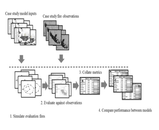
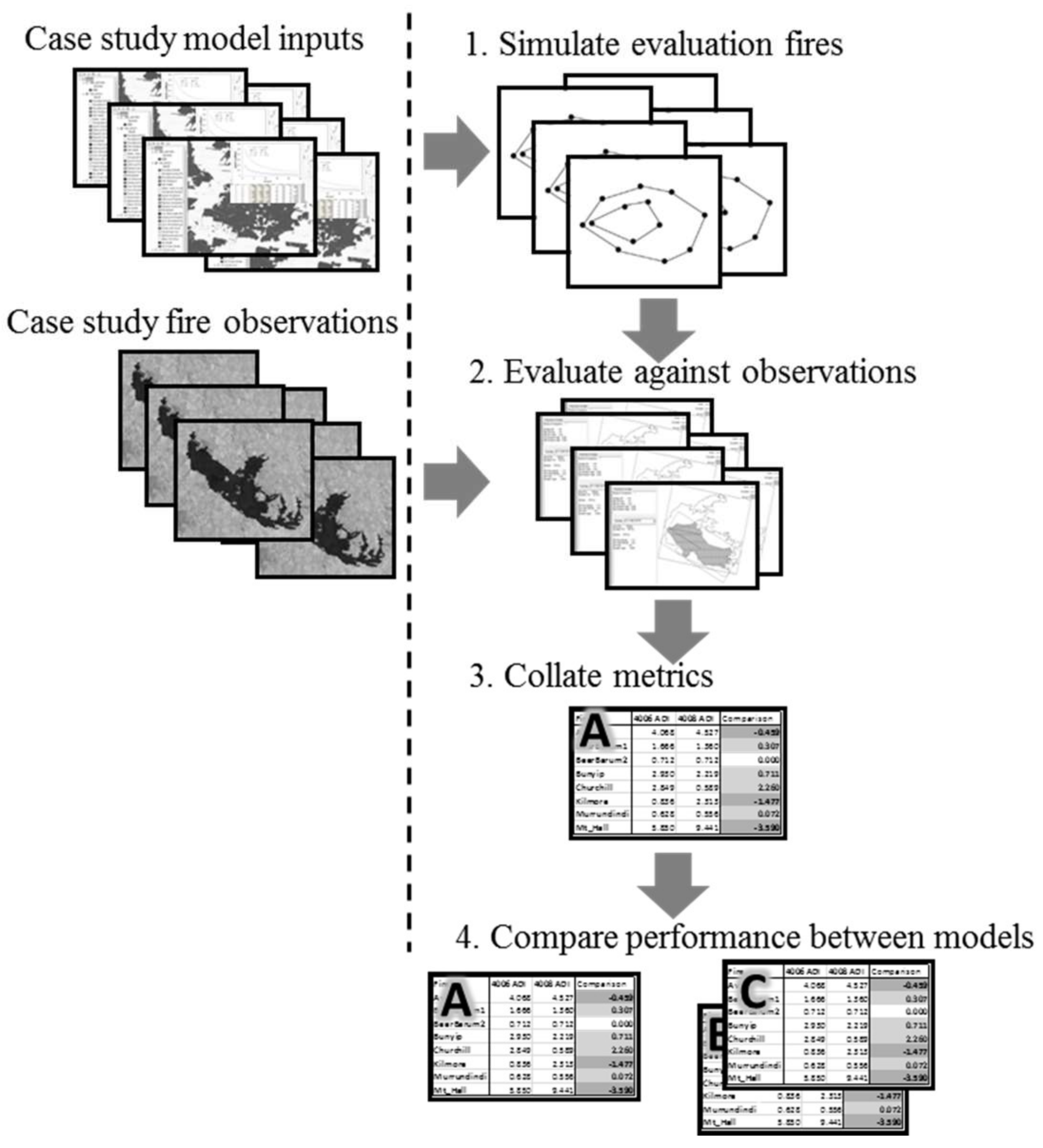
2.1. Overall Procedure

The following procedure was undertaken to compare the two model versions: compile an evaluation set of wildfires, simulate each fire with each model, quantitatively compare simulations against equivalent fire observations, and compile fire metrics to compare overall model performance. This procedure can compare models with very different formulations or requirements, as long as all necessary simulation model inputs are available. The procedure is presented graphically in Figure 1. Each stage is described in further detail below.

2.2. The Evaluation Set

The evaluation set of fires were sourced from large wildfire events that occurred in Australia in the states of Victoria, South Australia and Queensland. From the corresponding fire management agency in each state, the following data were sourced:
  • Observations of fire perimeters in the form of time stamped polygons that were derived from verifiable sources such as infra-red linescans [59] or official reconstructions;
  • Vegetation maps from which fuel classifications were derived using the relevant lookup table for each state;
  • Fire history maps indicating previously burned areas (for the moderation of fuel loads where recent fires had occurred [60]);
  • High (30 m) resolution digital elevation models (to derive terrain).
Weather observations from the fire’s locality during its occurrence were obtained in the form of automatic weather stations (AWS) records from the Australian Bureau of Meteorology. Fire suppression was not analysed or simulated as part of this project. Fires that had been used in prior model calibration were excluded from the evaluation set.

2.3. Test Models

To demonstrate the proposed method, we compared two versions of PHOENIX [10], a Hugyens based fire simulator developed for use in Australian wildland vegetation, including forests and grasslands. PHOENIX has been adopted for use throughout Australia by land management agencies for decision support [10,60,61] and for evaluating landscape fire risk [17]. It is routinely used to provide operational decision support during wildfires by producing faster-than-real-time predictions of fire progression. The PHOENIX software is developed using a progressive versioning process, whereby substantial changes are indicated with a new version number. Models with higher version numbers can be considered to have had further development than those with lower version numbers. The majority of model versions are used in internal development; version 4.007 has been used operationally, 4.008 is a development version only.
In this study, the primary difference between the two versions of the model is the treatment of the proportion forest fuel available to burn (as defined by Drought Factor, DF [5,62]). In the earlier version (4.007), the DF used for simulations is sourced from historic weather measured or modelled for a point or locality; the same DF value is applied regardless of topography. In the second version (4.008), an adjustment of the DF is applied, where it (and consequent fuel availability) is modified to be wetter or drier depending on local topography (in relation to solar radiation) and vegetation structure (where dense forest canopies are presumed to retard the rate of drying in surface fuels) [63,64]. The experimental algorithm is based on hypothesised processes and has not been tested with measured data. It is presented in Appendix A. Some minor code modifications to PHOENIX were made to allow performance metrics to be collated. These related to the data handling of outputs only and did not alter predictive function.

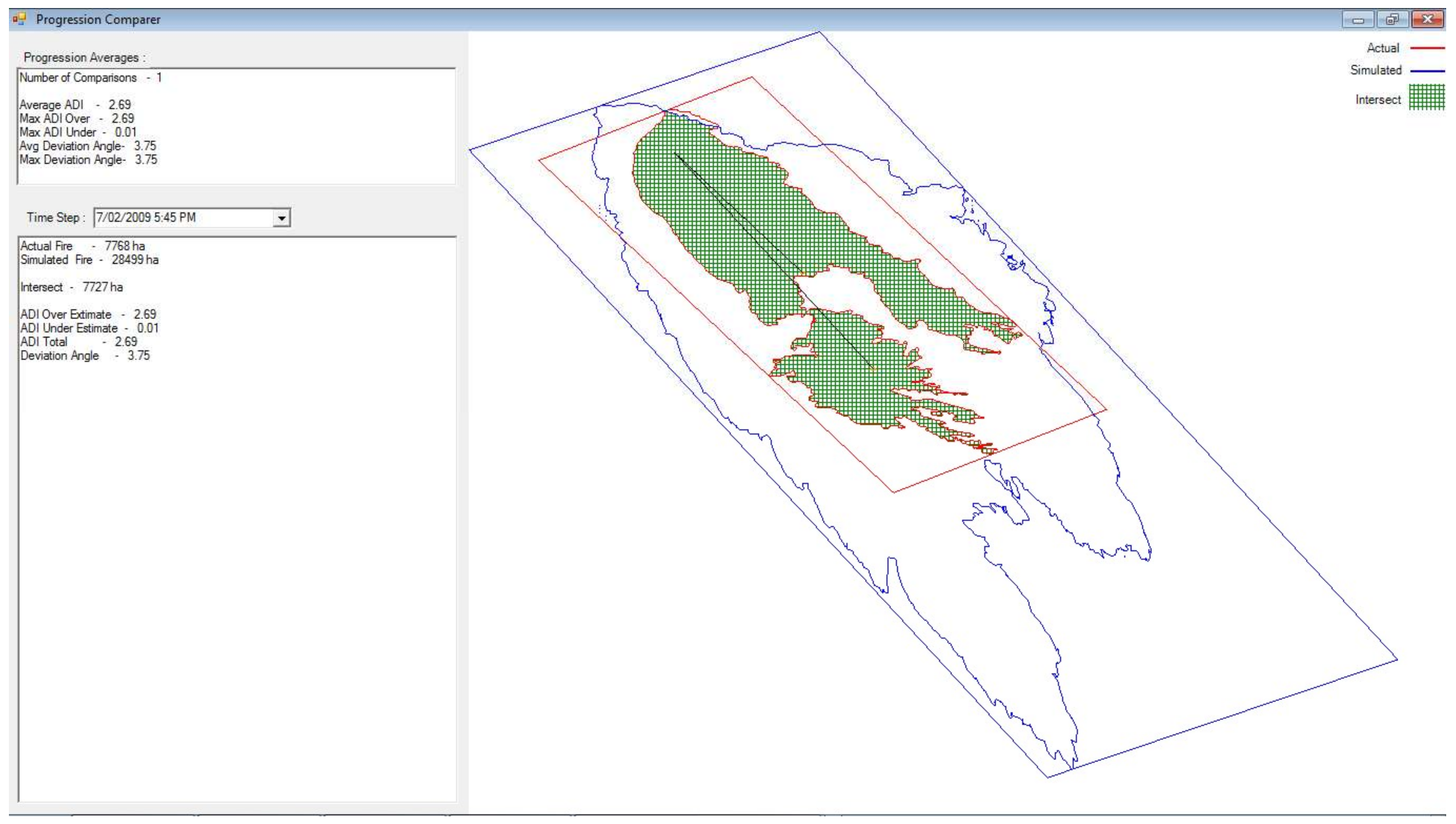
2.3.1. Evaluation Metrics

Objective metrics are necessary for a quantitative evaluation of model performance. To demonstrate the framework, we used indices of overlap to evaluate the fit of the simulation with each fire; the Area Difference Index (ADI, [65])—as a full index and decomposed into components of under and over-prediction. The ADI is a dimensionless ratio of the area incorrectly predicted to have been burnt relative to the correctly predicted area. The ADI is calculated as:
A D I ( t ) = O E ( t ) + U E ( t ) I ( t )
where for a point in time (t), the overestimated area (OE—area predicted to be burnt, but not actually burnt) and underestimated area (UE area predicted to be unburnt, but burnt) are divided by the correctly predicted area (I). The index scales linearly from ~0 to ∞, values closer to zero being better. It does not require that a domain be defined, so it is an index rather than a unit value. The decomposed indices, ADIover and ADIunder, indicate bias by considering only proportional area overestimated and underestimated relative to the correctly predicted area. To evaluate possible remnant issues with inputs (in particular, wind direction), the spread deviation angle was also calculated. The spread deviation angle was calculated by finding the difference between the predominant spread directions of the observed and predicted fires [18]. The predominant spread directions were determined by finding the direction of a line from the ignition point through the area-weighted geographic centre of each fire. The calculation of the evaluation metrics was coded into the versions of PHOENIX being evaluated.

2.3.2. Evaluation Process

For each fire, a burnt area observation from a single point in time was selected for comparison. A common pattern of fire propagation in eastern Australia is for fires to spread rapidly under strong northerly winds before a sudden south westerly wind change [31]. This results in a rapidly increasing fire area, with area increasing in proportion to the initial forward spread distance (as the entire flank of the fire becomes the head). This makes area-based performance metrics exceptionally sensitive to issues with the timing and strength of the wind change. In practice, understanding that state of the fire when the wind change occurs is a key requirement for managers as it has implications for firefighting strategy and safety. To reduce the sensitivity of predictions to the exact timing of the wind change, all fires were simulated to the point in time immediately before the occurrence of the wind change. Hence the evaluation was of the ability of the models to predict the fire to a particular state of interest to management; it was not a prediction of the capacity of the model to emulate the entire fire. Being able to predict at times of fast moving spread is typically a higher priority for operational use. Fire suppression was not simulated in the model; fire suppression was not a feature of any of the fires evaluated except for the Stawell fire [18], which was known to be influenced by suppression post wind change, however this was outside the time evaluated in this study.
Only a single comparison was made for each fire. A summary of the fires used for model evaluation are presented in Table 1 and brief descriptions of the fires are provided in Table 2. All fires were simulated separately with both versions of the model and the ADI values and deviation angles were compared.

3. Results

The two model variants successfully simulated all fires in the evaluation set. Figure 2 shows a screenshot taken from PHOENIX 4.008 demonstrating the within-model calculation of the performance metrics. The resultant metrics for version 4.007 and 4.008 are presented in Table 3 and Table 4 respectively.
The total predicted area burned with the downscaled version of the PHOENIX (4.008) was smaller than 4.007, as was the total area of intersection between the observed and predicted fires. However, the 4.008 also exhibited improved performance in terms of both total areas of underprediction (ADIunder) and overprediction (ADIover). Deviation angle was consistent between the two model versions, except for Beechworth, which showed an increase in error in 4.008.
The differences between the two model versions are shown in Table 5. The relative performance of the model with and without downscaled DF did not change greatly, with a Pearson’s correlation of 0.83 between the ADI scores. Both models seem to be underpredicting spread, although the degree of underprediction was not consistent across all fires—three fires in version 4.007 had substantial underpredictions, with ADIunder values that were greater than 2; Avoca, Beechworth and Churchill. In 4.008, the Churchill prediction was greatly improved.
When comparing the performance of the two versions of the model, the sum of the ADI values across all fires for version 4.007 was 21.03 and 4.008 was 16.61. The decrease of 4.42 units indicates an improvement in performance with the newer model, however when comparing the changes statistically, a paired t test for means indicated that these differences were not significant at the 0.05 level (n = 9, t = 1.66, p (two tailed) = 0.136). This test has relatively low power due to the number of fires used—increasing the number of fires in the evaluation set would increase the ability of the assessment processes to discriminate differences in performance amongst models.
When looking at individual fires, there was a performance improvement in version 4.008 for 5 of the 9 fires, a performance decline for 3 fires and 1 fire (Beerburrum) was unchanged. The Churchill fire had the greatest improvement (2.26 units.). Overall, the model performance change varied greatly between fires and aggregate performance measure was influenced by large changes in a small number of fires.

4. Discussion

The approach demonstrated here enabled two versions of PHOENIX to be objectively evaluated. Both models were similar in predictive performance, with the newer version found to be performing slightly (though not statistically significantly) better. As fire simulations are complex and non-linear, it can be expected that with any model adjustment, some fires will be predicted less accurately. This was found to be the case; the performance of PHOENIX 4.008 was not a unanimous improvement, with some fires (3 of 9) predicted more poorly. While the results infer an overall improvement, due to the small sample size this is not conclusive. As the newer version of the model has increased complexity, the modifications are not necessarily a parsimonious improvement. This highlights the issue of needing appropriate numbers of fires in the evaluation set before robust conclusions can be made. The ability to distinguish small changes in model performance is important, as in software development, there are many decisions that have the potential to alter predictive performance even when they do not alter the fundamental algorithms being used. For example, the degree of precision used in computations or the method of interpolation used in reading gridded spatial data can be important determinants of processing time, but may also have unintended effects on calculated outcomes [66].
To detect subtle differences between models, high statistical power is necessary. A disadvantage of using wildfire observations is that conditions are uncontrolled, they occur in diverse landscapes, they consume spatially heterogeneous vegetation, they are driven by changing weather conditions, [67] and are often affected by human interference (i.e., suppression). Consequently, data are noisy; the typical way to resolve such power issues is to increase the sample size [68]. In the case of this study, a power analysis of the need to resolve a difference of 1 ADI unit in the aggregate scores in the case study data (type I > 0.05, Power = 0.95, standard deviation = 1.04) would require at least 29 fires. There are substantial challenges to increasing the sample sizes for analysis, as wildfires occur with limited warning and it is difficult to obtain high-quality information due to their hazardous and ephemeral nature. Information must be collected opportunistically when wildfires occur, limiting the rate at which it can be collected. We used a small set of real fire observations; however, the information for these was derived from fires that occurred over a period of 24 years. To be able to identify specific limitations and weaknesses of the model; for example, issues in performance for particular vegetation types or at weather extremes, it is important to obtain sufficient replication of observations where the issue occurs. This may also be important when looking to evaluate performance in new regions, as some simulator inputs—particularly fuel—require local parameterisations. Additionally, climate change may lead to novel fuel and weather combinations that are outside the model development domain. Consequently, obtaining wildfire data for model assessment is critical. A wildfire evaluation set would ideally consist of a large number of well documented fires, however the development of such a dataset is challenging. Ideally, to resolve this, the data collection process for fires would be integrated into existing fire management systems so that information is systematically collected to a particular minimum standard [69]. To develop a systematic model evaluation system for fire simulators, at a minimum, the following information would be required:
  • Isochrones depicting the progression of the fire as a function of time;
  • Spatial datasets describing the terrain, vegetation/fuel properties and recent fire/disturbance history;
  • Weather observations from near the fire; in particular, temperature, relative humidity, wind speed and direction;
  • Information about the state of landscape dryness, such as direct measurements or dryness indices calculated from prior observed weather;
  • Details about suppression activities, including location, timing, methods used and effectiveness.
Where possible, it would be useful to store additional accessory information that can be used to provide insight into model performance issues and fire behaviour. For example, to verify modelled processes such as convection plumes it may be useful to record atmospheric (balloon) traces, observations of fire dynamics (for example the presence of pyrocumulus or ember storms), post fire severity maps and aerial imagery [69]. The spatial and temporal resolutions required of this information depend on the properties of the phenomena being modelled. If being able to simulate small-scale, transient or rapidly changing phenomena is important, it would be necessary to ensure that information is recorded at appropriate resolutions. To increase the information leverage of this data, there is the potential to evaluate model performance multiple times within a single fire event; i.e., by focusing on phenomena in independent parts of the fires (as determined by distinct changes in fuel or weather) rather than the fires in their entirety [50]. As the size of an evaluation set becomes large, there are opportunities for iterative model calibration rather than just evaluation. This is where a model can be run over the set, evaluated, adjusted and re-run. A large number of fires would be necessary for calibration, so that there are sufficient combinations of environmental conditions to allow the sources of error to be correctly apportioned. More importantly, calibrating on a small number of fires would increase the likelihood that models are overfit to the data and thus not suitable for generalisation [70].
When assessing models for development, having accurate input information is important. To achieve this, some form of human supervision will remain necessary. Poor quality information will add noise to evaluations of predictive performance and will limit the precision of objective comparison outcomes. To resolve this, the creation of minimum data quality standards for inputs would be a valuable first step. In doing this, it would be important to keep the data quality evaluation independent of the fire simulation process. It is difficult to verify the quality of some accessory model inputs (in particular, estimates of wind speed and direction) by solely viewing tables of data—fire simulations can provide a rapid visual indication of possible issues. However, using a model to audit case study reconstruction quality is disingenuous, as it could result in feedback that positively reinforces biases of the existing operational model. Using curated fire data to evaluate models, limits the influence of noisy data. However, it needs to be recognised that outcomes represent idealised performance where real-world forecast uncertainty is limited and are not necessarily representative of operational results.
This study compared two versions of a fire simulator aggregate performance metrics. As these are dependent on the fires used in their calculation, they are relative, not global—they are a function of the fires used in their computation. Consequently, all models must be tested with the same evaluation set if results are to be comparable. Figure 1 describes a four-step process; ideally this process would be continual with progressive updating as new fires occur and are added to the set. The evaluations in this study were based on an index of correctly predicted area at a single point in time. This is a coarse measure that contains limited information on the process of propagation; consequently, the model may be achieving the ‘correct’ results for the wrong reason. Other criteria or a combination of criteria can be included to account for this, such as considering rate of spread, intensity metrics or dynamic indices of performance (those that assess predictive congruence through time as well as space [51]). While this may result in a number of disparate indices when calculating the aggregate performance, these can be combined and weighted based on relative importance. For example, FROS performance may be weighted more heavily than area (which is in part a function of lateral spread). Alternatively, the influence of unusual fires may be reduced by calculating logarithmic rather than arithmetic means or using non-linear indices such as Jaccard’s Coefficient [65].
In addition to the aggregate performance metrics, the individual metrics for each fire still have some information that can be used to guide model development and provide an indication of potential areas for improvement. In this case, the partial performance indices (ADIover and ADIunder) were valuable in highlighting the nature of error. For example, the fire that had the greatest performance improvement was Churchill. This fire occurred in mountainous terrain, which is likely to have the strongest contrasts in topography and vegetation [64] and correspondingly would have the most to gain by including their effects. In contrast to this, the three fires that showed a decrease in predictive performance (Avoca, Redesdale and Stawell) all occurred in flatter terrain that was broken up by areas of grassland (Table 2.) This is suggestive that the downscaling algorithm used in PHOENIX 4.008 may be retarding landscape drying excessively in moderate terrain.
It should be noted that the method presented here allows the comparison of predictive performance with a perspective of model development. The application of this method to demonstrate improved predictive performance does not mean that a new model can be considered validated for operational use. When considering operational uses of models, criteria other than predictive performance may also be important to recognise in validation. For example, operational considerations may require recognition of a simulators ease of use, speed, reliability, software interoperability, data requirements, stability, sensitivity to inputs, hardware requirements and licensing. True validation would require that a range of these criteria are evaluated and can be demonstrated to meet minimum standards. Recognising that the model development process needs to consider measures other than predictive performance is a key step in considering operationalisation of research—for example, overly sensitive detection and warning systems do not necessarily meet the needs of users as there may be excessive rates of false positives [71]. It is feasible that performance metrics such as those demonstrated could be used to benchmark models, with acceptance criteria set based on performance thresholds. Such validation would require recognition of the intended use of the model—here we have evaluated the model in terms of its representation of fast moving wildfires. Alternative criteria would be necessary for other uses such as predicting fire behaviour within prescribed burns [72]. Additionally, demonstrated improvement of a performance metric does not necessarily represent a verification of model processes—the parameterisation of the algorithm incorporated into PHOENIX 4.008 is hypothetical and does not have a fundamental physical or empirical basis. In order to use an evaluation set of fires for fire simulator development, it is important to continue to advance our theoretical understanding of wildfire behaviour so that development can occur in a logical manner.

5. Conclusions

This study demonstrates a method for the quantitative, objective evaluation of relative performance of two different versions of a fire simulator. Such a process is important for software development—particularly to extend models to conditions beyond their original development range. There is an increasing reliance on wildfire simulation models for decision making; it is important that their level of development is suited for the conditions under which they are used. The need to predict fire behaviour under increasingly extreme conditions and climate driven novel fuel/weather combinations has already driven the intended use of many operational models beyond the conditions for which they were designed. We have demonstrated the potential to systematically use wildfire data to evaluate models and suggest that all fire simulation models should be subjected to this type of objective evaluation as part of the development process before being relied upon for decision making. The approach presented here represents a framework for evaluation – the evaluation criteria and metrics required for such a process will be a function of the intended uses of the model being assessed.

Acknowledgments

This work was undertaken as part of the project ‘Victorian Spatial and Temporal Drought Index and Drought Factor’ which was funded by an Australian National Disaster Resilience Scheme grant via the Victorian Department of Environment, Land, Water and Planning. Components of this work were supported by the Bushfire and Natural Hazards Cooperative Research Centre. Data were sourced from: The Victorian Department of Environment, Land, Water and Planning; The South Australian Department of Environment, Water and Natural Resources; Queensland Fire and Emergency Services; and the Australian Bureau of Meteorology. The software used for fire comparisons and simulation was PHOENIX RapidFire, a system developed at the University of Melbourne. The versions used were 4.007 and 4.008. The software is not currently available as a public product. It can be made available on agreement for research purposes; to enquire about access to the model for research use, please contact Phoenix Fire Predictions Limited, Level 1, 340 Albert Street, East Melbourne, Australia 3002, [email protected]. We would like to acknowledge the contribution of our reviewers, whose suggestions greatly improved this work.

Author Contributions

Thomas J. Duff and Kevin G. Tolhurst conceived the ideas behind the manuscript. Thomas J. Duff and Brett Cirulis undertook data collation and analysis. Thomas J. Duff was responsible for writing, drafting and review of the manuscript, with additional input from Jane G. Cawson, Petter Nyman, Gary J. Sheridan and Kevin G. Tolhurst.

Conflicts of Interest

The authors declare no conflict of interest. The founding sponsors had no role in the design of the study; analyses, or interpretation of data; in the writing of the manuscript, or in the decision to publish the results. The founding sponsors were responsible for collecting the raw data used in this study.

Appendix A

The landscape moisture in PHOENIX RapidFire is represented by Drought Factor (DF). In version 4.007, DF is calculated using the McArthur Mark 5 fire danger calculations [5]. In version 4.008, there are two adjustments to this.
The first adjustment component is to account for the effect that the forest canopy has drying processes. The canopy is represented in the model using the wind reduction factor (currently a mapped fuel attribute). This is where a fixed reduction factor is applied to reduce open 10 m wind speeds to a slower sub-canopy speed (i.e., with a factor of 3 applied, sub-canopy wind speed is 1/3 the open 10 m wind speed). Forests with dense canopies have higher factors applied. Radiative drying is a function of forest density, so wind reduction and radiative drying are assumed to be correlated [63] and so wind reduction factor is used as a proxy for drying potential. This adjustment decreases the DF in more closed forest and increases it in more open forests. The adjustment is represented by the equation:
C1 = (0.0046W2 − 0.0079W − 0.0175) × kbdi + (−0.9167W2 + 1.5833W + 13.5)
where C1 is correction factor 1, W is wind reduction factor and kbdi is the Keetch Byram Drought Index.
The second adjustment is used to account for the effect of azimuth at small scales, with the assumption that westerly and northerly aspects will undergo more rapid drying than southerly aspects. Azimuth is calculated using a digital elevation model and is used to apply an adjustment when slope exceeds 10°. This adjusts the DF by up two units depending on the azimuth. A sinusoidal curve is assumed, however for programming simplicity this is applied using a polynomial.
C2 = (2.204 × 1094 + (9.95 × 1073 + (6.34 × 1052 + 1.8
Where C2 is correction factor 2 and α is azimuth in degrees. The correction factors are applied to the drought factor as follows:
D F a d j u s t e d = D F × C 1 + C 2 10
where DFadjusted is the corrected drought factor, and DF is drought factor. DFadjusted is constrained between 0 and 10.

References

  1. Krawchuk, M.A.; Moritz, M.A. Constraints on global fire activity vary across a resource gradient. Ecology 2011, 92, 121–132. [Google Scholar] [CrossRef] [PubMed]
  2. Bradstock, R.A. A biogeographic model of fire regimes in Australia: Current and future implications. Glob. Ecol. Biogeogr. 2010, 19, 145–158. [Google Scholar] [CrossRef]
  3. Gill, A.M.; Stephens, S.L.; Cary, G.J. The worldwide “wildfire” problem. Ecol. Appl. 2013, 23, 438–454. [Google Scholar] [CrossRef] [PubMed]
  4. McLoughlin, D. A framework for intergrated emergency management. Public Adm. Rev. 1985, 45, 165–172. [Google Scholar] [CrossRef]
  5. Noble, I.R.; Gill, A.M.; Bary, G.A.V. McArthur’s fire-danger meters expressed as equations. Austral Ecol. 1980, 5, 201–203. [Google Scholar] [CrossRef]
  6. Rothermel, R.C. How to Predict the Spread and Intensity of Forest and Range Fires; Forest Service, U.S. Department of Agriculture: Boise Idaho, ID, USA, 1983.
  7. Sullivan, A.L. Wildland surface fire spread modelling, 1990–2007. 3: Simulation and mathematical analogue models. Int. J. Wildland Fire 2009, 18, 387–403. [Google Scholar] [CrossRef]
  8. Sullivan, A.L. Wildland surface fire spread modelling, 1990–2007. 1: Physical and quasi-physical models. Int. J. Wildland Fire 2009, 18, 349–368. [Google Scholar] [CrossRef]
  9. Finney, M.A. FARSITE: Fire Area Simulator—Model. Development and Evaluation; Rocky Mountain Reseach Station, Forest Service, U.S. Department of Agriculture: Missoula, MT, USA, 2004.
  10. Tolhurst, K.G.; Shields, B.; Chong, D. PHOENIX: Development and application of a bushfire risk management tool. Aust. J. Emerg. Manag. 2008, 23, 47–54. [Google Scholar]
  11. Tymstra, C.; Bryce, R.W.; Wotton, B.M.; Taylor, S.W.; Armitage, O.B. Development and Structure of Prometheus: The Canadian Wildland Fire Growth Simulation Model; Canadian Forest Service: Edmonton, AB, Canada, 2010. [Google Scholar]
  12. Tolhurst, K.G.; Duff, T.J.; Chong, D.M. From “Wildland-Urban Interface” to “Wildfire Interface Zone” using dynamic fire modelling. In Proceedins of the 20th International Congress on Modelling and Simulation, Adelaide, Australia, 1–6 December 2013; Piantadosi, J., Anderssen, R.S., Boland, J., Eds.; Modelling and Simulation Society of Australia and New Zealand: Adelaide, Australia, 2013; pp. 290–296. [Google Scholar]
  13. Finney, M.A.; Sapsis, D.B.; Bahro, B. Use of FARSITE for Simulating Fire Supression and Analyzing Fuel Treatment Economics. In Proceedings of the Conference on Fire in California Ecosystems: Integrating Ecology, Prevention and Management, San Diego, CA, USA, 17–20 November 1997; Sugihara, N.G., Morales, M.E., Morales, T.J., Eds.; Association for Fire Ecology: San Diego, CA, USA, 2002; pp. 121–136. [Google Scholar]
  14. Alcasena, F.; Salis, M.; Ager, A.; Castell, R.; Vega-García, C. Assessing wildland fire risk transmission to communities in Northern Spain. Forests 2017, 8, 30. [Google Scholar] [CrossRef]
  15. Mallinis, G.; Mitsopoulos, I.; Beltran, E.; Goldammer, J. Assessing Wildfire Risk in Cultural Heritage Properties Using High Spatial and Temporal Resolution Satellite Imagery and Spatially Explicit Fire Simulations: The Case of Holy Mount Athos, Greece. Forests 2016, 7, 46. [Google Scholar] [CrossRef]
  16. Ager, A.A.; Vaillant, N.M.; Finney, M.A.; Preisler, H.K. Analyzing wildfire exposure and source–sink relationships on a fire prone forest landscape. For. Ecol. Manag. 2012, 267, 271–283. [Google Scholar] [CrossRef]
  17. Department of Environment and Primary Industries. Victorian Bushfire Risk Profiles: A Foundational Framework for Strategic Bushfire Risk Assessment; The State of Victoria Department of Environment and Primary Industries: East Melbourne, Australia, 2013.
  18. Duff, T.J.; Chong, D.M.; Taylor, P.; Tolhurst, K.G. Procrustes based metrics for spatial validation and calibration of two-dimensional perimeter spread models: A case study considering fire. Agric. For. Meteorol. 2012, 160, 110–117. [Google Scholar] [CrossRef]
  19. Alexander, M.E.; Cruz, M.G. Are the applications of wildland fire behaviour models getting ahead of their evaluation again? Environ. Model. Softw. 2013, 41, 65–71. [Google Scholar] [CrossRef]
  20. Sullivan, A.L. Wildland surface fire spread modelling, 1990–2007. 2: Empirical and quasi-empirical models. Int. J. Wildland Fire 2009, 18, 369–386. [Google Scholar] [CrossRef]
  21. Johnston, P.; Kelso, J.; Milne, G.J. Efficient simulation of wildfire spread on an irregular grid. Int. J. Wildland Fire 2008, 17, 614–627. [Google Scholar] [CrossRef]
  22. Rothermel, R.C.; Rinehart, G.C. Field Procedures for Verification and Adjustment of Fire Behaviour Predictions; Forest Service, U.S. Department of Agriculture: Ogden, UT, USA, 1983.
  23. Hoffman, C.M.; Canfield, J.; Linn, R.R.; Mell, W.; Sieg, C.H.; Pimont, F.; Ziegler, J. Evaluating crown fire rate of spread predictions from physics-based models. Fire Technol. 2016, 221–237. [Google Scholar] [CrossRef]
  24. Anderson, W.R.; Cruz, M.G.; Fernandes, P.M.; McCaw, L.; Vega, J.A.; Bradstock, R.A.; Fogarty, L.; Gould, J.; McCarthy, G.; Marsden-Smedley, J.B.; et al. A generic, empirical-based model for predicting rate of fire spread in shrublands. Int. J. Wildland Fire 2015, 24, 443–460. [Google Scholar] [CrossRef]
  25. Cheney, N.P.; Gould, J.S.; McCaw, W.L.; Anderson, W.R. Predicting fire behaviour in dry eucalypt forest in southern Australia. For. Ecol. Manag. 2012, 280, 120–131. [Google Scholar] [CrossRef]
  26. Rothermel, R.C. A Mathematical Model. for Predicting Fire Spread in Wildland Fuels; Forest Service, U.S. Department of Agriculture: Ogden, UT, USA, 1972.
  27. Cruz, M.G.; Alexander, M.E.; Sullivan, A.L. Mantras of wildland fire behaviour modelling: Facts or fallacies? Int. J. Wildland Fire 2017, 26, 973–981. [Google Scholar] [CrossRef]
  28. Papadopoulos, G.D.; Pavlidou, F.N. A comparative review on wildfire simulators. IEEE Syst. J. 2011, 5, 233–243. [Google Scholar] [CrossRef]
  29. Thaxton, J.M.; Platt, W.J. Small-scale fuel variation alters fire intensity and shrub abundance in a pine savanna. Ecology 2006, 87, 1331–1337. [Google Scholar] [CrossRef]
  30. Riccardi, C.L.; Ottmar, R.D.; Sandberg, D.V.; Andreu, A.; Elman, E.; Kopper, K.; Long, J. The fuelbed: A key element of the Fuel Characteristic Classification System. Can. J. For. Res. 2007, 37, 2394–2412. [Google Scholar] [CrossRef]
  31. Long, M. A climatology of extreme fire weather days in Victoria. Aust. Meteorol. Mag. 2006, 55, 3–18. [Google Scholar]
  32. Viegas, D.X. Fire line rotation as a mechanism for fire spread on a uniform slope. Int. J. Wildland Fire 2002, 11, 11–23. [Google Scholar] [CrossRef]
  33. Sharples, J.J.; McRae, R.H.D.; Wilkes, S.R. Wind–terrain effects on the propagation of wildfires in rugged terrain: Fire channelling. Int. J. Wildland Fire 2012, 21, 282–296. [Google Scholar] [CrossRef]
  34. Sharples, J.J.; Mills, G.A.; McRae, R.H.D.; Weber, R.O. Foehn-like winds and elevated fire danger conditions in southeastern Australia. J. Appl. Meteorol. Clim. 2010, 49, 1067–1095. [Google Scholar] [CrossRef]
  35. Haines, D.A. A lower atmospheric severity index for wildland fires. Natl. Weather Dig. 1988, 13, 23–27. [Google Scholar]
  36. McRae, R.H.D.; Sharples, J.J.; Wilkes, S.R.; Walker, A. An Australian pyro-tornadogenesis event. Nat. Hazards 2013, 1801–1811. [Google Scholar] [CrossRef]
  37. Sun, R.; Krueger, S.K.; Jenkins, M.A.; Zulauf, M.A.; Charney, J.J. The importance of fire–atmosphere coupling and boundary-layer turbulence to wildfire spread. Int. J. Wildland Fire 2009, 18, 50–60. [Google Scholar] [CrossRef]
  38. Viegas, D.; Simeoni, A. Eruptive behaviour of forest fires. Fire Technol. 2011, 47, 303–320. [Google Scholar] [CrossRef] [Green Version]
  39. Cruz, M.G.; Sullivan, A.L.; Gould, J.S.; Sims, N.C.; Bannister, A.J.; Hollis, J.J.; Hurley, R.J. Anatomy of a catastrophic wildfire: The Black Saturday Kilmore East fire in Victoria, Australia. For. Ecol. Manag. 2012, 269–285. [Google Scholar] [CrossRef]
  40. Alexander, M.E.; Cruz, M.G. Evaluating a model for predicting active crown fire rate of spread using wildfire observations. Can. J. For. Res. 2006, 36, 3015–3028. [Google Scholar] [CrossRef]
  41. Jakeman, A.J.; Letcher, R.A.; Norton, J.P. Ten iterative steps in development and evaluation of environmental models. Environ. Model. Softw. 2006, 21, 602–614. [Google Scholar] [CrossRef]
  42. Bennett, N.D.; Croke, B.F.W.; Guariso, G.; Guillaume, J.H.A.; Hamilton, S.H.; Jakeman, A.J.; Marsili-Libelli, S.; Newham, L.T.H.; Norton, J.P.; Perrin, C.; et al. Characterising performance of environmental models. Environ. Model. Softw. 2013, 40, 1–20. [Google Scholar] [CrossRef]
  43. Stratton, R.D. Guidance on Spatial Wildland Fire Analysis: Models, Tools, and Techniques; RMRS-GTR-183; Rocky Mountain Research Station, Forest Service, USDA: Fort Collins, CO, USA, 2006; p. 15. [Google Scholar]
  44. Perry, G.L.W. Current approaches to modelling the spread of wildland fire: A review. Prog. Phys. Geog. 1998, 22, 222–245. [Google Scholar] [CrossRef]
  45. Sá, A.C.L.; Benali, A.; Fernandes, P.M.; Pinto, R.M.S.; Trigo, R.M.; Salis, M.; Russo, A.; Jerez, S.; Soares, P.M.M.; Schroeder, W.; et al. Evaluating fire growth simulations using satellite active fire data. Remote Sens. Environ. 2017, 190, 302–317. [Google Scholar] [CrossRef]
  46. Feunekes, U. Error Analysis in Fire Simulation Models. M.Sc. Thesis, University of New Bruswick, Fredericton, NB, Canada, 1991. [Google Scholar]
  47. Cui, W.; Perera, A.H. Quantifying spatio-temporal errors in forest fire spread modelling explicitly. J. Environ. Inform. 2010, 16, 19–26. [Google Scholar] [CrossRef]
  48. Green, D.G.; Gill, A.M.; Noble, I.R. Fire shapes and the adequacy of fire-spread models. Ecol. Model. 1983, 20, 33–45. [Google Scholar] [CrossRef]
  49. Fujioka, F.M. A new method for the analysis of fire spread modeling errors. Int. J. Wildland Fire 2002, 11, 193–203. [Google Scholar] [CrossRef]
  50. Duff, T.J.; Chong, D.M.; Tolhurst, K.G. Quantifying spatio-temporal differences between fire shapes: Estimating fire travel paths for the improvement of dynamic spread models. Environ. Model. Softw. 2013. [Google Scholar] [CrossRef]
  51. Filippi, J.-B.; Mallet, V.; Nader, B. Representation and evaluation of wildfire propagation simulations. Int. J. Wildland Fire 2014, 23, 46–57. [Google Scholar] [CrossRef]
  52. Peltier, L.J.; Haupt, S.E.; Wyngaard, J.C.; Stauffer, D.R.; Deng, A.; Lee, J.A.; Long, K.J.; Annunzio, A.J. Parameterizing mesoscale wind uncertainty for dispersion modeling. J. Appl. Meteorol. Clim. 2010, 49, 1604–1614. [Google Scholar] [CrossRef]
  53. Valero, M.M.; Rios, O.; Mata, C.; Pastor, E.; Planas, E. An integrated approach for tactical monitoring and data-driven spread forecasting of wildfires. Fire Saf. J. 2017. [Google Scholar] [CrossRef]
  54. Zhang, C.; Rochoux, M.; Tang, W.; Gollner, M.; Filippi, J.-B.; Trouvé, A. Evaluation of a data-driven wildland fire spread forecast model with spatially-distributed parameter estimation in simulations of the FireFlux I field-scale experiment. Fire Saf. J. 2017, 91, 758–767. [Google Scholar] [CrossRef]
  55. Rochoux, M.C.; Delmotte, B.; Cuenot, B.; Ricci, S.; Trouvé, A. Regional-scale simulations of wildland fire spread informed by real-time flame front observations. Proc. Combust. Inst. 2013, 34, 2641–2647. [Google Scholar] [CrossRef]
  56. Kelso, J.K.; Mellor, D.; Murphy, M.E.; Milne, G.J. Techniques for evaluating wildfire simulators via the simulation of historical fires using the Australis simulator. Int. J. Wildland Fire 2015, 24, 784–797. [Google Scholar] [CrossRef]
  57. Filippi, J.B.; Mallet, V.; Nader, B. Evaluation of forest fire models on a large observation database. Nat. Hazards Earth Syst. Sci. 2014, 14, 3077–3092. [Google Scholar] [CrossRef] [Green Version]
  58. Faggian, N.; Bridge, C.; Fox-Hughes, P.; Jolly, C.; Jacobs, H.; Ebert, E.E.; Bally, J. Final Report: An. Evaluation of Fire Spread Simulators Used in Australia; Australian Bureau of Meterology: Melbourne, Australia, 2017. [Google Scholar]
  59. Billing, P. Operational Aspects of the Infrared Line Scanner; Department of Conservation and Environment: Victoria, Australia, 1986.
  60. Paterson, G.; Chong, D. Implementing the Phoenix Fire Spread Model for Operational Use. In Proceedings of the Surveying and Spatial Sciences Biennial Conference 2011, Wellington, New Zealand, 21–25 November 2011; New Zealand Institute of Surveyors and the Surveying and Spatial Sciences Institute: Wellington, New Zealand, 2011. [Google Scholar]
  61. Duff, T.J.; Chong, D.M.; Cirulis, B.A.; Walsh, S.F.; Penman, T.D.; Tolhurst, K.G. Understanding risk: Representing fire danger using spatially explicit fire simulation ensembles. In Advances in Forest Fire Research; Viegas, D.X., Ed.; Imprensa da Universidade de Coimbra: Coimbra, Portugal, 2014; pp. 1286–1294. [Google Scholar]
  62. Finkele, K.; Mills, G.A.; Beard, G.; Jones, D.A. National gridded drought factors and comparison of two soil moisture deficit formuations used in prediction of Forest Fire Danger Index in Australia. Aust. Meteorol. Mag. 2006, 55, 183–197. [Google Scholar]
  63. Walsh, S.F.; Nyman, P.; Sheridan, G.J.; Baillie, C.C.; Tolhurst, K.G.; Duff, T.J. Hillslope-scale prediction of terrain and forest canopy effects on temperature and near-surface soil moisture deficit. Int. J. Wildland Fire 2017, 26, 191–208. [Google Scholar] [CrossRef]
  64. Nyman, P.; Sherwin, C.B.; Langhans, C.; Lane, P.N.J.; Sheridan, G.J. Downscaling regional climate data to calculate the radiative index of dryness in complex terrain. Aust. Met. Ocean. J. 2014, 64, 109–122. [Google Scholar] [CrossRef]
  65. Duff, T.J.; Chong, D.M.; Tolhurst, K.G. Indices for the evaluation of wildfire spread simulations using contemporaneous predictions and observations of burnt area. Environ. Model. Softw. 2016, 83, 276–285. [Google Scholar] [CrossRef]
  66. Duff, T.J.; Chong, D.M.; Tolhurst, K.G. Using discrete event simulation cellular automata models to determine multi-mode travel times and routes of terrestrial suppression resources to wildland fires. Eur. J. Oper. Res. 2015, 241, 763–770. [Google Scholar] [CrossRef]
  67. Pastor, E.; Zárate, L.; Planas, E.; Arnaldos, J. Mathematical models and calculation systems for the study of wildland fire behaviour. Prog. Energ. Combust. 2003, 29, 139–153. [Google Scholar] [CrossRef]
  68. Stockwell, D.R.B.; Peterson, A.T. Effects of sample size on accuracy of species distribution models. Ecol. Model. 2002, 148, 1–13. [Google Scholar] [CrossRef]
  69. Duff, T.J.; Chong, D.M.; Cirulis, B.A.; Walsh, S.F.; Penman, T.D.; Tolhurst, K.G. Gaining benefits from adversity: The need for systems and frameworks to maximise the data obtained from wildfires. In Advances in Forest Fire Research; Viegas, D.X., Ed.; Imprensa da Universidade de Coimbra: Coimbra, Portugal, 2014; pp. 766–774. [Google Scholar]
  70. Hawkins, D.M. The problem of overfitting. J. Chem. Inf. Comput. Sci. 2004, 44, 1–12. [Google Scholar] [CrossRef] [PubMed]
  71. Fonollosa, J.; Solórzano, A.; Marco, S. Chemical sensor systems and associated algorithms for fire detection: A review. Sensors 2018, 18, 553. [Google Scholar] [CrossRef] [PubMed]
  72. Loschiavo, J.; Cirulis, B.; Zuo, Y.; Hradsky, B.A.; Di Stefano, J. Mapping prescribed fire severity in south-east Australian eucalypt forests using modelling and satellite imagery: A case study. Int. J. Wildland Fire 2017, 26, 491–497. [Google Scholar] [CrossRef]
Figure 1. Framework for comparing and improving fire simulation models using an evaluation set of case study fires.
Forests 09 00189 g001
Figure 2. Screengrab of fire model comparison from PHOENIX RapidFire 4.008 (University of Melbourne, Parkville, Australia) for the Bunyip fire. Observed fire area is presented as a green polygon, simulated fire area is presented as a blue polygon.
Forests 09 00189 g002
Table 1. The evaluation set of fires used for evaluating the performance of the fire simulator, PHOENIX RapidFire.
Fire NameLocalityStart DateStart TimeSimulated UntilBurnt (ha)
AvocaVictoria14 January 198513:5019:0021,147
BeechworthVictoria7 February 200917:552:00 110,939
Beerburrum Day 2Queensland7 November 199412:5018:002472
BunyipVictoria7 February 200912:2017:457768
ChurchillVictoria7 February 200913:2018:155802
MurrindindiVictoria7 February 200914:4018:1521,757
RedesdaleVictoria7 February 200914:4518:003850
StawellVictoria31 December 200516:442:00 17511
WangarySouth Aust.11 January 200516:3014:3045,810
1 simulated into the following day
Table 2. General descriptions of the fires used for evaluating PHOENIX RapidFire.
Fire NameDescription
AvocaDry eucalypt forest/grazing agricultural land mix, relatively flat terrain, moderate spotting
BeechworthDry eucalypt forest/pine plantation, undulating terrain, moderate spotting
Beerburrum Day 2Eucalypt forest/pine plantation, undulating terrain, substantial spotting
BunyipWet and dry eucalypt forest, hilly terrain, substantial spotting
ChurchillPine and eucalypt plantation, wet eucalypt forest, mountainous terrain, substantial spotting
MurrindindiGrassland/wet and dry eucalypt forest, rural residential areas, mountainous terrain, very substantial spotting
RedesdaleGrazing with some remnant eucalypts, undulating terrain, minimal spotting.
StawellGrazing/cropping/remnant dry eucalypt forest patches, undulating terrain, rural residential areas, minimal spotting. Fire suppression in grasslands limited flank spread
WangaryMainly grazing/cropping farmland, undulating terrain, minimal spotting
Table 3. Performance metrics for PHOENIX RapidFire without downscaling (version 4.007, University of Melbourne, Parkville, Australia) simulating fires from the evaluation set. The values presented are simulated fire area, area of intersection between the simulated and observed fires, the deviation in predominant spread direction, and the Area Difference Indices (ADI; proportion of underprediction, overprediction and total error relative to correctly predicted area).
Fire NameSimulated (ha)Intersection (ha)Deviation (°)ADIunderADIoverADI
Avoca417341734.324.070.004.07
Beerburrum Day 22807194712.500.270.440.71
Bunyip30,36577346.750.002.932.93
Churchill152215102.172.840.012.85
Murrindindi25,81318,1731.870.200.420.62
Redesdale384830123.710.280.280.56
Beechworth311917595.415.220.775.99
Wangary33,77132,7244.140.400.030.43
Stawell21,62459842.110.262.612.87
Total127,04277,016 13.547.4921.03
Table 4. Performance metrics for PHOENIX RapidFire with downscaling (version 4.008, University of Melbourne, Parkville, Australia) simulating fires from the evaluation set. The values presented are simulated fire area, area of intersection between the simulated and observed fires, the deviation in predominant spread direction, and the Area Difference Indices (ADI; proportion of underprediction, overprediction and total error relative to correctly predicted area).
Fire NameSimulated (ha)Intersection (ha)Deviation (°)ADIunderADIoverADI
Avoca382738274.054.530.004.53
Beerburrum Day 22807194712.500.270.440.71
Bunyip24,76877125.470.012.212.22
Churchill469140530.790.430.160.59
Murrindindi 28,46119,6481.240.110.450.56
Redesdale272325152.820.530.080.61
Beechworth7939272714.913.011.914.92
Wangary 26,73226,0663.950.760.030.78
Stawell12,35753830.490.401.301.69
Total114,30573,877 10.056.5816.61
Table 5. Differences between ADI metrics between PHOENIX RapidFire version 4.007 and the downscaling 4.008. Negative values indicate an improvement. Decreases in performance are shown in bold.
Fire NameΔADIunderΔADIoverΔADI
Avoca0.460.000.46
Beerburrum Day 20.000.000.00
Bunyip0.01−0.72−0.71
Churchill−2.410.15−2.26
Murrindindi−0.090.03−0.06
Redesdale0.25−0.200.05
Beechworth−2.211.14−1.07
Wangary0.360.000.35
Stawell0.14−1.31−1.18
Total−3.49−0.91−4.42

