Article

Spatial Prediction of Wildfire Susceptibility Using Field Survey GPS Data and Machine Learning Approaches

1
Department of Geoinformatics–Z_GIS, University of Salzburg, 5020 Salzburg, Austria
2
Department of Remote Sensing and GIS, University of Tabriz, Tabriz 5166616471, Iran
3
Discipline of Geography and Spatial Sciences, University of Tasmania, Hobart 7005, Australia
4
Research Center for Digital Mountain and Remote Sensing Application, Institute of Mountain Hazards and Environment, Chinese Academy of Sciences, Chengdu 610041, China
5
University of Chinese Academy of Sciences, Beijing 100049, China
6
Department of Geography, University of Zanjan, Zanjan 45371-38791, Iran
*
Author to whom correspondence should be addressed.
Submission received: 23 June 2019 / Revised: 22 July 2019 / Accepted: 24 July 2019 / Published: 28 July 2019

Abstract

:
Recently, global climate change discussions have become more prominent, and forests are considered as the ecosystems most at risk by the consequences of climate change. Wildfires are among one of the main drivers leading to losses in forested areas. The increasing availability of free remotely sensed data has enabled the precise locations of wildfires to be reliably monitored. A wildfire data inventory was created by integrating global positioning system (GPS) polygons with data collected from the moderate resolution imaging spectroradiometer (MODIS) thermal anomalies product between 2012 and 2017 for Amol County, northern Iran. The GPS polygon dataset from the state wildlife organization was gathered through extensive field surveys. The integrated inventory dataset, along with sixteen conditioning factors (topographic, meteorological, vegetation, anthropological, and hydrological factors), was used to evaluate the potential of different machine learning (ML) approaches for the spatial prediction of wildfire susceptibility. The applied ML approaches included an artificial neural network (ANN), support vector machines (SVM), and random forest (RF). All ML approaches were trained using 75% of the wildfire inventory dataset and tested using the remaining 25% of the dataset in the four-fold cross-validation (CV) procedure. The CV method is used for dealing with the randomness effects of the training and testing dataset selection on the performance of applied ML approaches. To validate the resulting wildfire susceptibility maps based on three different ML approaches and four different folds of inventory datasets, the true positive and false positive rates were calculated. In the following, the accuracy of each of the twelve resulting maps was assessed through the receiver operating characteristics (ROC) curve. The resulting CV accuracies were 74%, 79% and 88% for the ANN, SVM and RF, respectively.

1. Introduction

Monitoring forest ecosystems is a critical component of many governmental land management agencies [1,2]. Since forest ecosystems contain about 66% of the total terrestrial carbon, they are a significant component of the global carbon budget [3]. Forests are a vital component to maintaining an environmental balance and regulating the carbon cycle [4,5]. Forests are considered valuable natural resources in northern Iran because they play a significant role in supporting the local economy by harvesting forest products and supporting tourist activities. Wildfires are usually accompanied by severe episodes of smoke, which has adverse health impacts on communities [6]. As almost all of the forests in northern Iran are located in mountainous areas, they play a considerable role in the protection against some natural hazards, i.e., erosion and rock falls [7]. The wildfires affect vegetation, not only at the level of the individual bush or tree but also at the levels of the forest ecosystem and the landscape [8]. Though wildfires are commonly recognized as a natural part of a forest ecosystem, the increasing frequency of events, the increasing areas damaged by the fire, and the severity of wildfires present considerable challenges in forestry areas [9]. Various factors like wind, topography, and droughts have great impacts on fire occurrence and spread, but, in many cases, fires are caused by humans [10]. These fires endanger human life and can cause enormous destruction of buildings and infrastructure [11].
Global warming and climate change issues are considered as major factors contributing to these upwards trends. Recently, global warming has caused long term water stress during the summer season, which results in increased dryness in forest lands and, consequently, an increase in wildfires [12]. In turn, these fires produce gas emissions, which increase carbon dioxide and, ultimately, global warming [13]. Besides the natural factors, anthropogenic factors, i.e., the activities of local people and tourism, are also considered as wildfire conditioning factors in our study area [14]. Both natural and anthropogenic wildfire conditioning factors make it difficult for environmental organizations to predict wildfires, a difficulty which results in complications during combustion controlling responses. These responses are essential for effectively combating wildfires and reducing their harmful consequences [9]. In addition to environmental damages, wildfires have widespread economic and social impacts on the local people in our study area in northern Iran. Therefore, systematic research on prediction approaches for the wildfires and fire extents in this area is required. New tools and methods must be applied to improve wildfire management; in this regard, employing artificial intelligence (AI) may be considered an effective solution. AI technologies like machine learning (ML), which is a computational study of algorithms, can help scientists generate solid models for monitoring wildfires and discovering variances in real-time [10]. In automated learning approaches, ML acquires information from data, and ML algorithms receive the input data and implement statistical analyses to calculate new entries. The spatial prediction of an area’s susceptibility to any natural hazard requires data from geographic information systems (GIS) and remote sensing (RS) sources. Further to using relevant input data to wildfire susceptibility, an appropriate approach is required to effectively produce susceptibility maps [15].
Several studies have been conducted to develop a spatial prediction of wildfire susceptibility using GIS and RS, implemented in different approaches, such as fuzzy logic [16] and the analytical network process (ANP) [12]. However, recently, ML approaches have achieved fairly good results in various natural hazard susceptibility mapping studies. Some common ML approaches were applied in a wide range of studies in the field of wildfire modelling and susceptibility mapping such as an artificial neural network (ANN) [17], support vector machines (SVM) [18,19,20], and random forest (RF) [21,22], all three of which we evaluated in this study for the spatial prediction of wildfire susceptibility. We used the capabilities of these three ML approaches using sixteen wildfire conditioning factors based on five main factors—topographic, meteorological, anthropological, vegetation, and hydrological. The wildfire conditioning factors were selected according to the interpretations of similar studies that have examined the forests of northern Iran [14]. An inventory dataset of the polygons of the wildfires was prepared based on global positioning system (GPS) data (obtained from the state wildlife organization), and this was evaluated and enhanced by the thermal anomalies (hotspots) of a moderate resolution imaging spectroradiometer (MODIS) to train and validate the applied ML approaches. Concerning the spatial distribution of wildfire polygons, it is expected that the performance of our applied ML approaches is affected by the random selection of training data. The pixels of the inventory dataset were randomly divided into four different folds to use four-fold cross-validation (CV). Using CV is recommended to deal with the effects of randomness on the performance of any data mining and ML approaches [23,24]. Three out of the four folds were chosen for training the ML approaches. The remaining fold was used for the validation process. This process was repeated for all four folds of our wildfire inventory dataset. We also used GIS capabilities to combine layers with different spatial resolutions and to use overlay methodologies within the ML approaches. A total of twelve spatial prediction wildfire susceptibility maps were generated based on the ANN, SVM, and RF approaches using four different folds of the inventory dataset. Finally, the resulting susceptibility maps were validated based on the inventory dataset and a common accuracy assessment methodology.

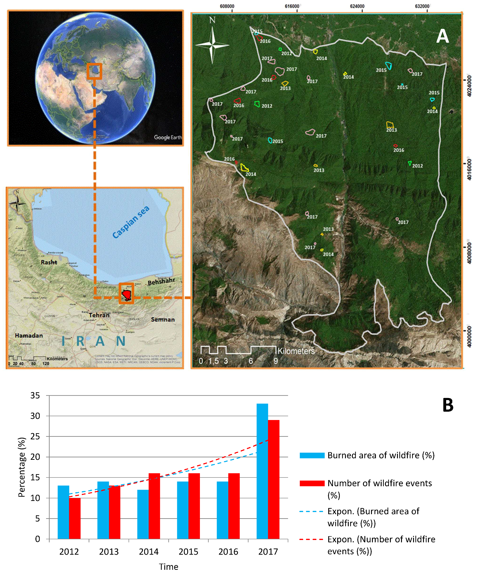
2. Overview of the Study Area

Mazandaran Province, with an area of 23,842 km2, is located on the southern coast of the Caspian Sea and covers 1.46% of Iran’s territory. Based on the census in 2016, it consists of 14 cities and is home to 3,374,725 persons. The province has a strategic location based on its sea borders with four countries, namely Russia, Azerbaijan, Turkmenistan, and Kazakhstan, as well as being located just to the north of Iran’s capital, Tehran. Mazandaran Province has diverse natural resources, including plains, forests, rainforest, and large reservoirs of oil and natural gas. The forestry area of Amol County, located in the center of Mazandaran Province, was selected as our study area (see Figure 1). It covers an area of about 646 km2 and is vital for the local economy by harvesting of forest products and animal husbandry. The study area is also considered as one of the popular areas for tourist activities because of its recreational centers, which attract people from all over the country, mostly during the summer. The forestry area of this county shares boundaries with other Mazandaran Province counties such as Nur County in the west and Babol County in the east. The elevation ranges from approximately 100 m in valleys to more than 2500 m above mean sea level in mountainous areas. This area has experienced several destructive wildfires during the last decade. More than 20 settlement areas and villages are located within the study area, mostly in valleys. Wildfires in Mazandaran Province have always been common. However, the total number and expansion area of wildfires grew during the study period. It is believed but not proven that the growing number and expansion of wildfires can be attributed to the increasing temperatures and droughts during the summer season.

3. Materials

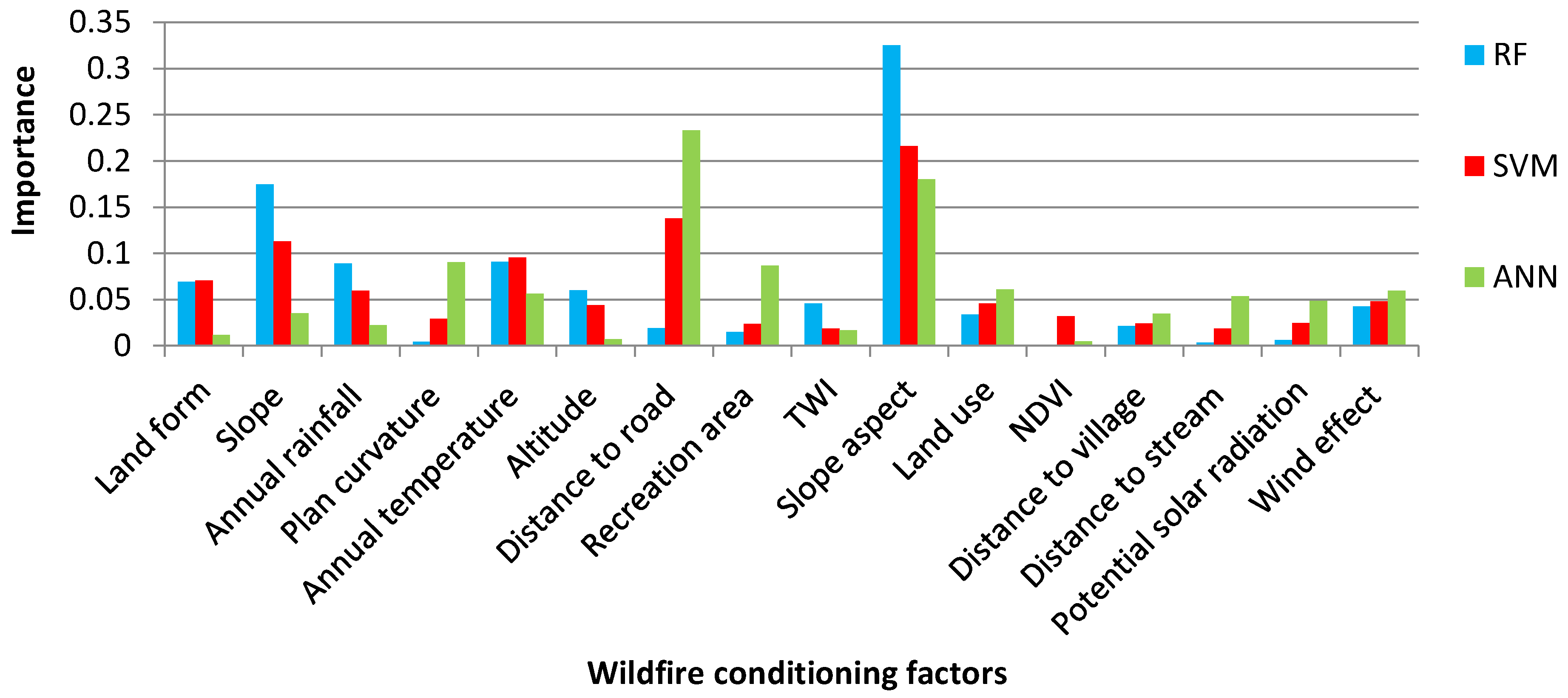
3.1. Conditioning Factors

In this subsection, we summarize the applied wildfire conditioning factors for Amol County. The topographic conditioning factors are the altitude, slope aspect, slope, plan curvature, landform, and the topographic wetness index (TWI) derived from the advanced spaceborne thermal emission and reflection radiometer (ASTER) global digital elevation model (GDEM) with an approximate resolution of 30 meters. The TWI was calculated to define the aspect of steady-state soil wetness, which can be calculated with the relevant equation outlined in Hong et al. (2016) [25]. The meteorological factors are annual temperature, potential solar radiation, and wind effect. The solar radiation varies from nearly 0.282 KWH / m 2 to more than 1.877 KWH / m 2 , and this range is classified in five classes based on natural breaks. The wind effect includes both wind speed and wind direction. The dry wind during summer and in September, in particular, is one of the main reasons for the spread of the fire [26]. The factor of wind effect was generated based on three different criteria, including the degree of wind direction, wind speed (m/s), and altitude layer. The wildfire conditioning vegetation factor was the normalized difference vegetation index (NDVI) [27]. The NDVI factor was generated for the highly vegetated period during the summer using Landsat-8 Operational Land imagery with a 30 × 30 m resolution (path 164, row 35, 17 June 2017) sourced from the United States Geological Survey (USGS) archive (http://earthexplorer.usgs.gov). As our case study area is part of a protected area in northern Iran, there is no deforestation and, therefore, no significant change in forest coverage has taken place over the last decade. Thus, there was no major alteration in the NDVI between 2012 and 2017.
The anthropological factors are the distance to the settlements, land use, and the distance to recreational areas and roads. In our case study area, human activities are responsible for many potential sources of wildfire ignition. Thus, the anthropological factors were selected as an essential group of the conditioning factor. The conditioning hydrological factors are annual rainfall and the distance to streams. The conditioning factors of the temperature and rainfall were prepared based on an annual mean. All applied factors were prepared as GIS layers with a resolution of 30 meters and classified based on their attributes and significance regarding wildfire susceptibility. Table 1, Table 2, Table 3, Table 4 and Table 5 show the conditioning factors, the area of each class, and percent of the wildfire-affected areas in each class; Table 6 indicates the relationships between factors and wildfire risk.

3.2. Generating a Wildfire Inventory Dataset

3.2.1. Data Source

Training any ML approach requires adequate input data and a reliable training dataset. We used freely available MODIS fire-event data (from 2012 to 2017) to generate an inventory dataset of the precise polygons of the wildfire-affected areas. MODIS fire products provide unique information like the time and spatial distribution of the fires. Burned areas in these products are represented by the removal of vegetation, deposits of charcoal and ash, and vegetation structure alteration, and the algorithms of burned area mapping benefit from such temporal, spectral, and structural changes.
MODIS is a twin sensor of the Terra and Aqua satellites, and its 36 electromagnetic spectral bands vary from visible bands to thermal infrared bands. Data are transmitted to the earth twice a day [45]. The hotspots of MODIS were applied in current related studies to specify the exact affected area and the time of the wildfires [46,47]. MODIS thermal fire products of MOD14 with a temporal resolution of five min and processing level-2 were used in this study. The Terra MODIS instrument acquires data twice daily (10:30 AM and PM). The collection number of the applied MODIS data was 6. The fire detection approach is based on an absolute finding of a fire when the fire strength is adequate to detect. The product includes fire occurrence area within fire pixels. A number of 34 hotspots were detected during the studied period in our study area. The spatial resolution of the hotspots used for identifying wildfires is 1 km, which shows a reasonably good approximated perimeter of the burned area. However, the resulting polygons were then manually enhanced using the GPS data for plausibility checks. The final wildfire inventory dataset was created using the GPS data from the field surveys and evaluated using the hotspots of MODIS. These corrections were manually done in the geographic information system ArcGIS 10.3. The GPS data are a result of an extensive field survey that was done by the state wildlife organization of Amol County (SWOAC) [48]. The resulting dataset from the SWOAC includes the polygons with detailed borders. However, they did not document all wildfire events, especially not the small ones. Thus, the small wildfire events were documented based on their dates using the MODIS dataset, while the GPS polygons were considered for the larger wildfires. The integration of both sources resulted in a more reliable inventory dataset representing the location and the area of the wildfires.

3.2.2. Dataset Organization

The four-fold CV was used to organize the dataset for training and testing the models. In this validation approach, the dataset D of wildfire pixels is randomly divided into mutually exclusive k-folds of D1, D2, …, Dk which ∀ n and mt, size Dn = size Dm. Then, the model is run k times and for any time of t, tk (see Figure 2). When the model is run at the time of t, the model is trained with dataset D without considering the subset of Dt, which remains for the validation of the model [49]. Since we randomly divided our inventory dataset into four folds, each time, 75% (13,066 pixels) was used to train the model, and 25% (4355 pixels) was reserved for the validation processes. The number of folds is selected based on different factors, including the complexity of the problem, the volume of the inventory dataset, and the methodology used. We used the CV method to deal with the adverse effects of randomness on the performances of the ML approaches for spatial prediction of wildfire susceptibility.

4. Methods

4.1. Overall Methodology

The workflow of this study for the spatial prediction of wildfire susceptibility in Amol County was as follows:
Preparing the conditioning factors based on five main factors, namely topographic, meteorological, anthropological, vegetation, and hydrological.
Generating a wildfire inventory dataset from the hotspots of MODIS data-enhanced using field survey GPS data.
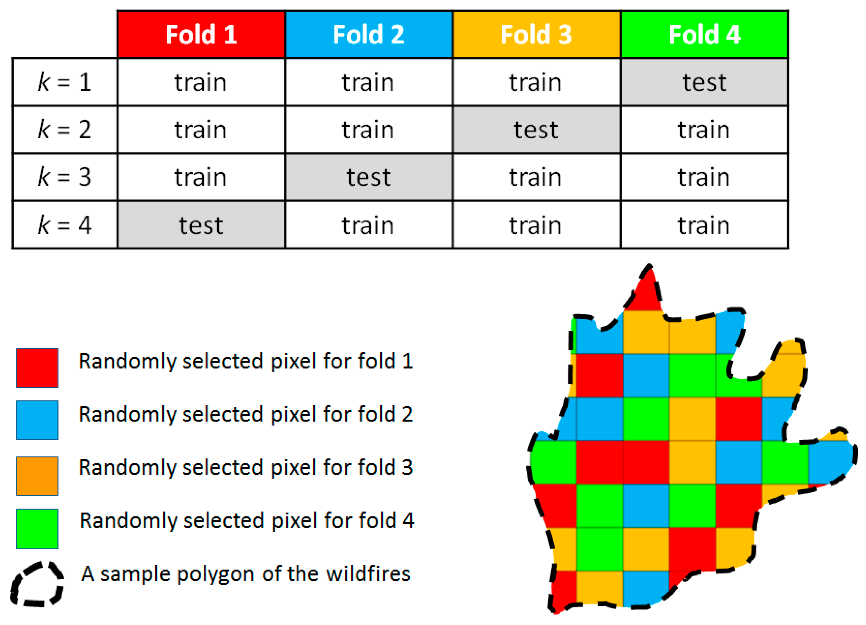
Using a four-fold CV and dividing the inventory dataset into four different equal-sized folds.
Applying the ANN, SVM and RF models for the spatial prediction of wildfire susceptibility, based on each fold of the training dataset.
Validating the performances of each ML approach using the receiver operating characteristics (ROC) curve.
The methodologies and the experimental results are organized in the following sections. Further descriptions and discussions regarding the use of different ML approaches and training datasets can be found in the discussions and conclusion section.

4.2. Artificial Neural Network (ANN)

An ANN mimics human brain performance by using a set of interconnected nodes [50,51]. The human brain is imitated in two ways: First, acquiring knowledge and information through a learning process; second, synaptic weights are used to store knowledge [52]. An ANN is trained to distinguish and generalize the connection between inputs and outputs. Generally speaking, there is a connection between the multi-input non-linear process from small individual interconnected neural networks and weighted interconnections (see Figure 3). An ANN can find an optimal solution for complex non-linear problems, such as the spatial prediction of wildfire susceptibility, by discovering their patterns among the conditioning factors and responses. Many neural network structures have been proposed in the literature for different purposes. We structured our ANN according to the most widely used structure using the multilayer perceptron (MLP) architecture and the back propagation algorithm (BPA) for the training. In the MLP architecture, neurons which exist in the same hidden layer are not connected. However, there are connections between the neurons of a layer and those of the next layer. The number and size of hidden layers in the ANN model are typically fixed for the particular application [53]. All initial weightings that were randomly chosen are updated by the repeated backward process to minimize the error [54]. The number of epochs and the learning rate of our model were set to 500 and 0.1, respectively.

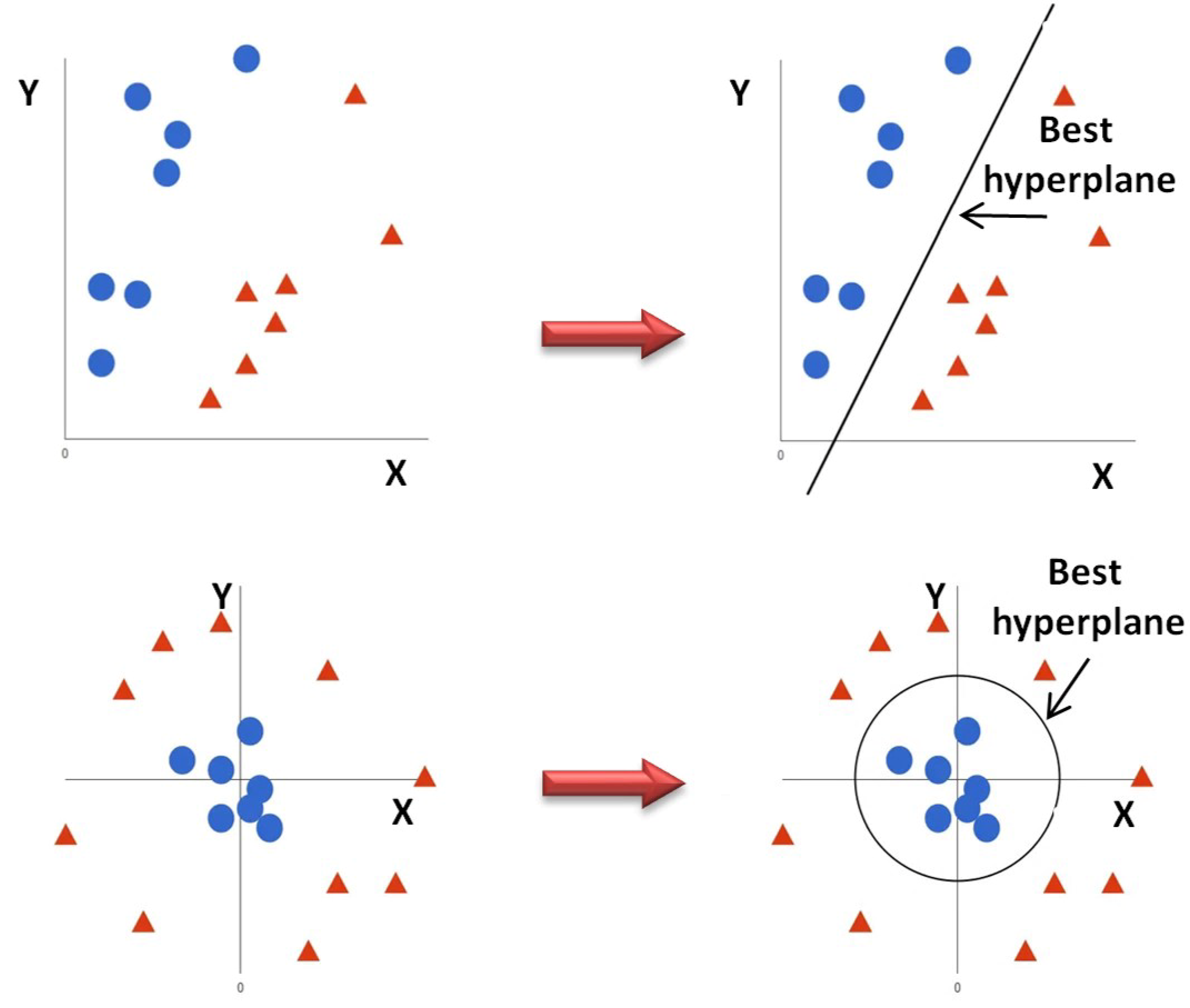
4.3. Support Vector Machines (SVM)

The SVM, which is known as the maximum-margin method [55], created by Hava Siegelmann and Vladimir Vapnik, is another ML that was applied in this study for the spatial prediction of wildfire susceptibility. It can provide a higher speed and better results with a limited number of data points. This approach is based on statistical learning theory that maps the dataset into a higher-dimensional feature space through non-linear transformers to specify the best separating hyperplane [51]. The best hyperplane will be found when the separating margins between the defined classes of the problem are maximal [56]. The kernel function of the radial basis function (RBF), which is considered as the most commonly used natural hazard susceptibility modelling approach, was used in our case study. The resulting susceptibility map based on SVM using the RBF kernel also depends on the kernel width (γ). The hyper-parameter γ controls the tradeoff between errors due to bias and variance, which defines how far the influence of a training sample reaches. The low values indicate ‘far,’ and high values indicate ‘close’ influence. This hyper-parameter is also the inverse of the radius of the influence of samples, which is designated by the model as support vectors. The regularization (C) parameter also influences the behavior of SVM. Thus, determining the optimal parameters is a crucial task [51]. A fairly good result was obtained using a γ of 0.95 and a C of 0.8. Concerning this γ, the algorithm of SVM was built using our input dataset and the corresponding fold of the inventory data to the spatial prediction of wildfire susceptibility for the entire study area. In general, SVM works (Figure 4) as follows:
(a).
It allows classifying linearly separable data.
(b).
If it is not linearly separable, it is possible to use the kernel trick to make it work.

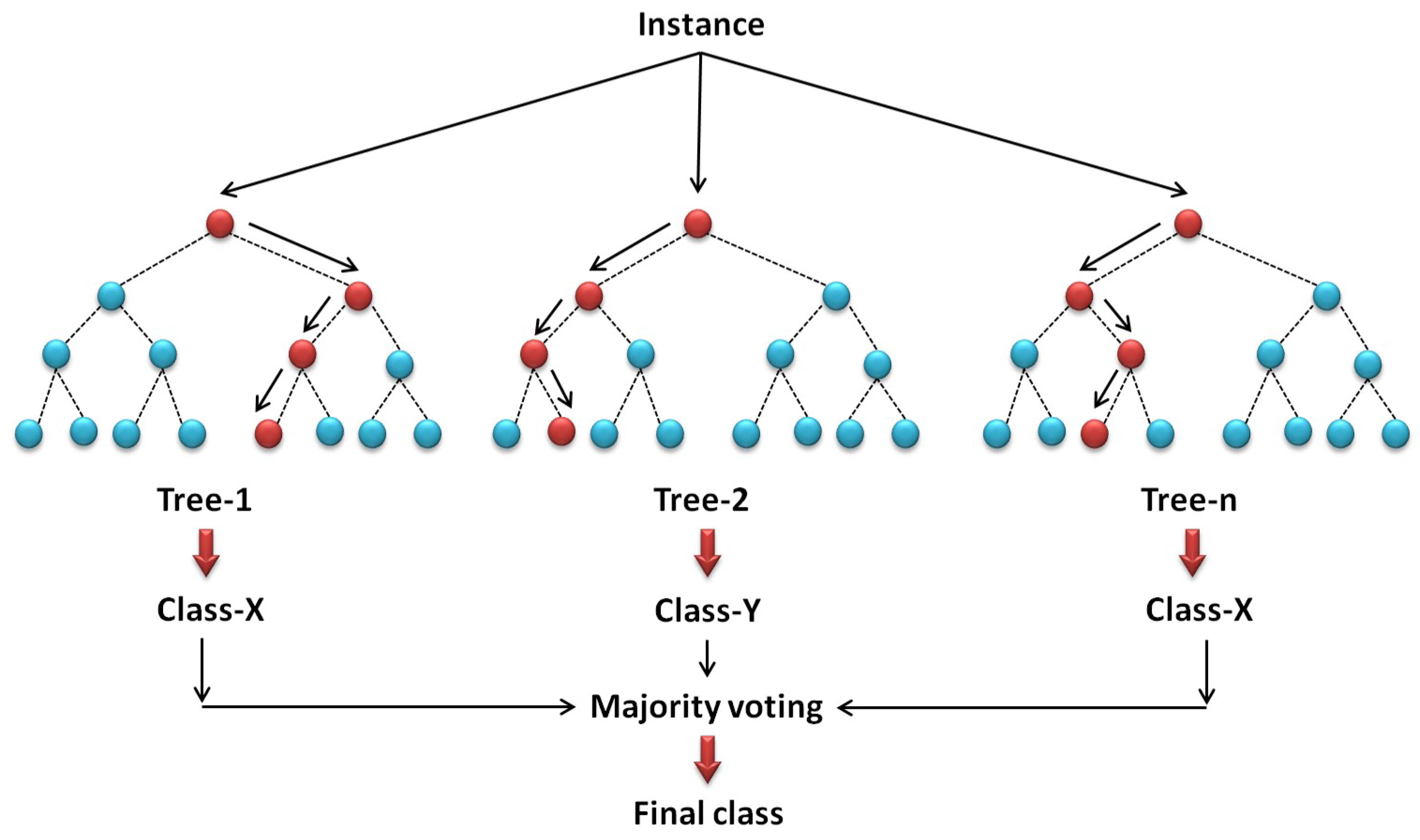
4.4. Random Forest (RF)
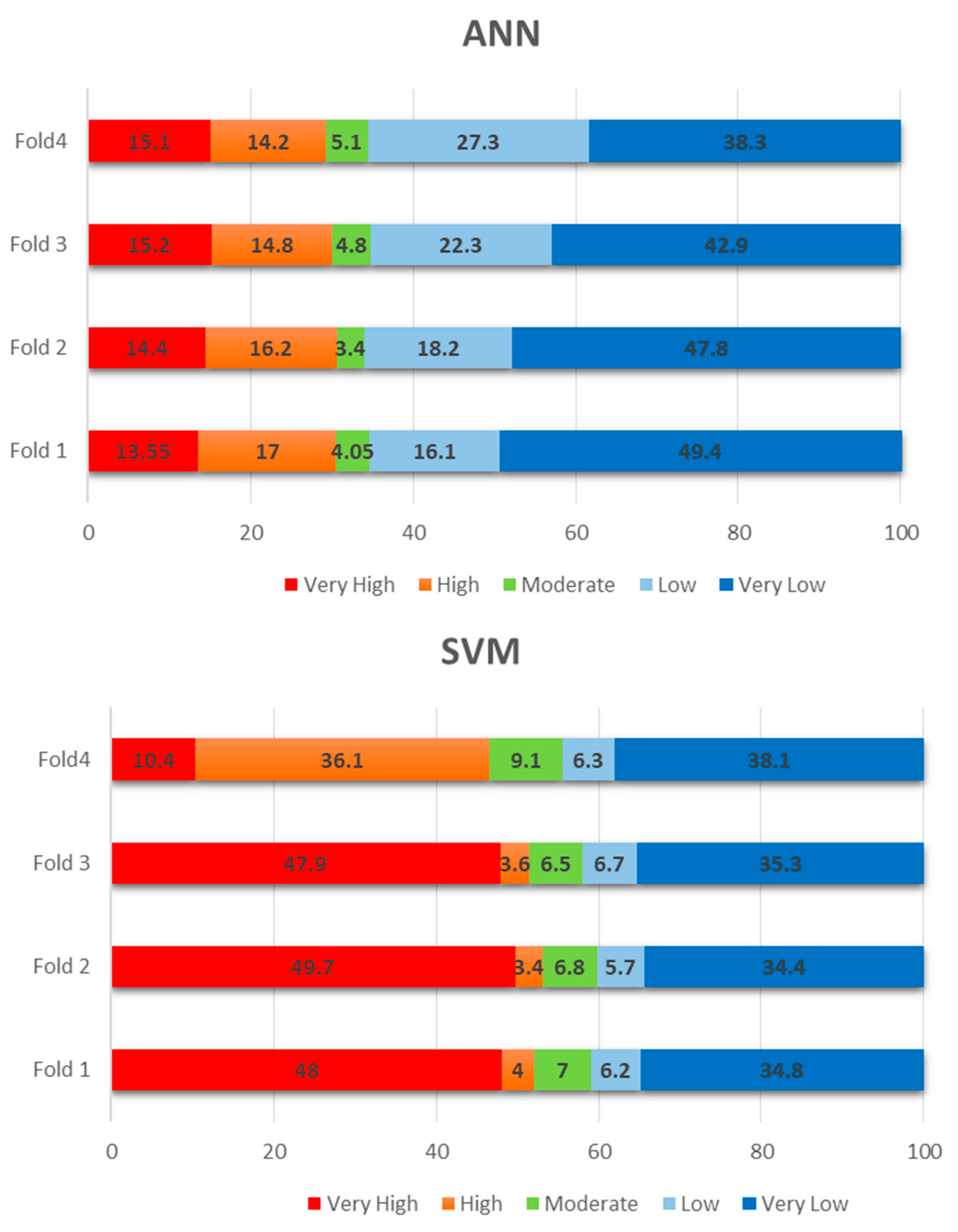
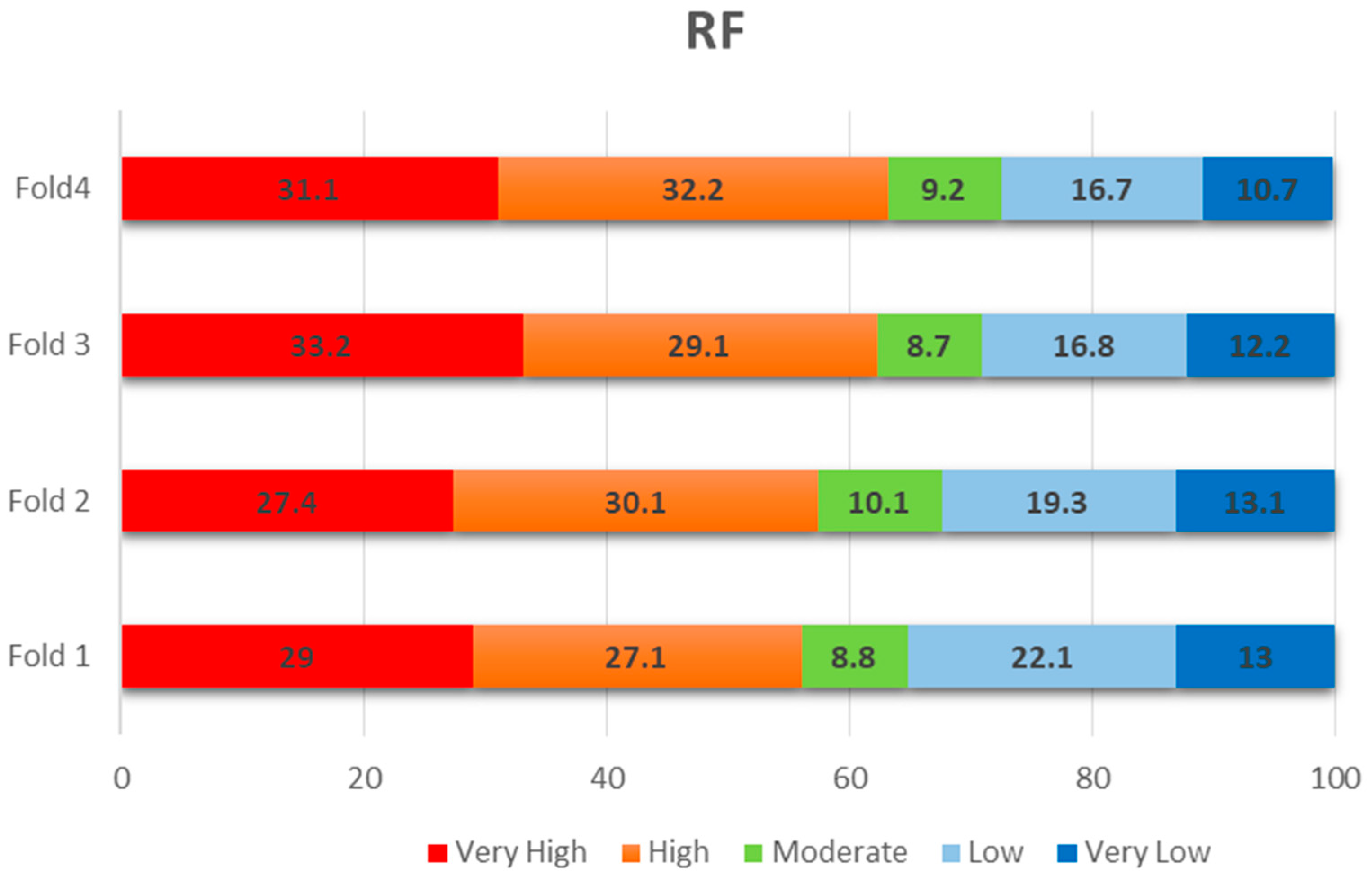
The RF ML approach, which was created by Ho (1994) [57] and developed by Breiman and Cutler (2001) [58], combines multiple decision trees for classification of the input dataset [59]. The training set overfitting of decision trees’ habit was corrected and covered by RF; it can also be described as a bunch of decision trees which take the input dataset and re-sample it several times based on the training data. In this method, tree bootstrap samples are created from the original dataset. Then, an unpruned classification or regression tree is established for each of the bootstrap samples. The outcome is the average of the results of all the trees (Figure 5). More specifically, a random set of features is selected at each stage when predicting an output, and each output is weighted by the value derived from the votes that it receives. The majority vote, based on the outputs of estimated decision trees, converge in a single decision tree for the final classification [60,61]. Using the single decision tree overcomes the uncertainty problem and results in a higher prediction accuracy [21]. Deriving the high variance from different decision trees is a crucial matter in the RF classification approach. The cited literature and others report RF classifications to yield good results for satellite image classifications. Hence, RF is considered to be one of the most operative non-parametric ensemble learning approaches in susceptibility modelling and mapping. Some basic training options for the RF model are the maximum number of trees, the number of variables to consider in split search, and the type of sampling process. The first two options consider in split searching of the RF. In this study, the maximum number of trees and the number of variables for each split were set to 1000 and 25, respectively. The maximum number of trees was selected based on a range from 500 to 2000, and the number of variables was the default value. The type of the sampling process is considered as a proportion which identifies what percentage of observations is applied for each tree. An out-of-the-bag (OOB) sample statistic was used for the final forest model. This sample statistic is a practical measure of how a model performs on new inputs. Thus, the inputs that are used in the training sample are called the bagged observations, and, consequently, the input data for a decision tree in the RF model are called the bagged data. The fraction of trees in the RF model required to vote for a specific given class is called the voting threshold or cutoff [62]. The cutoff fraction in our RF model was set to 0.01, which results in the minimum error rate. We repeated the re-sampling process 500 times to get the best result. This process was used for each of the four folds of our inventory dataset. All ML methods were done using the statistical analysis system (SAS), which is a comprehensive statistical analysis software package.

5. Results

The applied ML approaches using all mentioned conditioning factors and the inventory dataset were used for the spatial prediction of wildfire susceptibility for Amol County. The results from each ML approach were used to produce final susceptibility maps using GIS spatial analysis and data aggregation models. The resulting prediction maps based on three ML approaches and different training folds of the inventory dataset are shown in Figure 6, Figure 7 and Figure 8. The wildfire susceptibility maps represent a measure of the probability of the occurrence of wildfires for a region based on considered conditioning factors. The natural breaks classification method (available in Arc map 10.3) was used to classify the resulting spatial prediction of wildfire susceptibility maps. This classification method is the most common method for categorizing prediction maps for interpreting values close to each class boundary (e.g., values between ‘‘High’’ and ‘‘Very high’’ susceptibility predictions) [64].

Validation and Sensitivity Analyses

In this section, we outline a widely used accuracy assessment method which was used to evaluate the performance of the applied ML approaches by analyzing the conformity between the validation fold of the inventory dataset and the products of the applied approaches. The effectiveness of each ML approach was specified by evaluating any existing uncertainty among the resulting susceptibility maps. We applied the ROC curve method [65] using the 4355 wildfire inventory pixels (see Section 3.2.2) which were not used to train the applied ML approach. The ROC method is usually used for characterizing the quality of susceptibility prediction approaches. The plotted curves based on the ROC method show the trade-off between the false positive rate and the true positive rate on the X and Y axis, respectively. The area under the curve (AUC) was used as the accuracy index, and values close to one indicate that the resulting susceptibility map had a high accuracy. ROC curves were calculated for all resulting wildfire susceptibility maps, and Figure 6, Figure 7 and Figure 8 show the results of comparing the observed wildfires with the susceptibility maps based on a four-fold CV. The results of the AUC from the ROC method for all resulting wildfire susceptibility maps indicated accuracies above 71%, and the highest accuracy was achieved with the RF approach, which yielded an AUC value of more than 94%. However, the resulting CV accuracies were 74%, 79% and 88% for the ANN, SVM, and RF, respectively (see Table 7).
Figure 9 illustrates the estimated coefficient values for the wildfire conditioning factors by the applied ML models in their best performance regarding CV approach. The coefficients were normalized using the expression obtainable by Equation (1) [66].
W s , i ( k ) =   ( W i ( k ) min W i ( k ) ) / ( max W i ( k ) min W i ( k ) ) ,       k = 1 ,   2 ,   3
where W s , i ( k ) is the normalized weight at kth ML model, W i ( k ) is the resulting weight by the kth model, and i is the identification number of each conditioning factor. The resulting coefficient values show that the three wildfire susceptibility ML models were consistent in terms of some conditioning factors including slope aspect, annual temperature, land use, distance to villages and wind effect. The factor of slope aspect is the essential factor that contributes to wildfires in our study area, followed by distance to roads and slope. However, there was a vast difference between the importance of the distance to roads resulting in different ML models. Though the importance of this factor for the SVM and ANN was high, that of the RF model was an insignificant value of the coefficient. The coefficient value of slope for the RF model was the second most important among the other factors, whereas that of the ANN was a small value of the coefficient.

6. Discussion

Determining which model type to use for the prediction of wildfire susceptibility is essential, because the outcomes may help decision-makers to make the right decisions. Though wildfire prediction is difficult due to the spatial heterogeneity of conditioning factors, our modelling successfully showed the robust potentials of ML algorithms in this regard. Of the various available ML algorithms, those of RF, SVM, and the ANN have used to predicate spatial susceptibility in Amol. To reach our goal, our case study area was divided into six classes (from Very High to Very Low susceptibility to wildfires) for each algorithm. The results showed that areas with moderate risk had the lowest share in all three algorithms, whereby the highest rate of moderate risk was acquired by SVM, Fold 4, with only 9.1%. The maximum areas of the resulting maps based on the ANN model belong to very low risk, while those of SVM model were categorized in a very high-risk category. In RF, it was variable between areas with very high and high risks; in Fold 1 and Fold three, areas with very high risk were most prevalent; however, areas in the high range prevailed in Folds 2 and 4. On the other hand, considering the information presented in Figure 10, more than 60% of the case study areas in the ANN were identified as being at very low and low risks of wildfire. In contrast, high and very high ranges covered almost more than 65% of the area in RF, and the wildfire risk category in SVM was almost equal between areas, with very low and very high forming more than 80% of the measures.
Previous studies suggested that ML algorithms can be more appropriate than statistical methods for wildfire studies. Generally, for ROC–AUC, the rates range from 0 to 1; values of <0.6 are defined as poor, values between 0.6 < 0.7 are moderate, values between 0.7 < 0.8 are good, values between 0.8 < 0.9 are very good, and, finally, excellent performance is indicated by values higher than 0.9. In this study, we found that the performance of RF was outstanding (very close to an excellent rate with 88% CV accuracy), while SVM and the ANN illustrated good performances. Among all folds, as Table 2 illustrates, RF and SVM had the best results in Fold 3 with 94% and 82%, respectively, while the ANN experienced the best result in Fold 4 with 79%. Folds 2 and 4 were the places where RF showed the lowest CV accuracy with 85%, and the lowest SVM accuracy was achieved in Fold 4 with 75%; meanwhile, the ANN yielded the lowest accuracy in Fold 2 with 71%. Compared to the previous studies, Rodrigues and de la Riva (2014) [67] have pointed out that ML models, particularly RF, can enhance the prediction of wildfire accuracy compared to traditional methods. Jaafari and Pourghasemi (2019) [68] mentioned SVM, with an AUC value of 83%, as performing well for the spatial modelling of wildfire probability, and Bui et al. (2017) [69] reported an AUC value of 0.88% for SVM. Thus, it seems that the results are different based on region and factors.
After analyzing the spatial location of the wildfires that occurred from 2012 to 2017 and the conditioning factors through the sensitivity analysis, it was revealed that the slope aspect factor was more critical than the other factors to identifying the very high or high wildfire risks. Distance to roads was considered as an important factor based on the resulting maps from the ANN model. To link the villages to each other, which are located in the case study area, roads were extended almost across the forest, particularly the north-east section, where more than 55% of wildfires occurred in the past. Moreover, with an increase in distance from forests to roads, the number of wildfires decreased, illustrating that forests that are closer to recreation areas had a higher risk of fire occurrence. Many types of research have shown increased fire ignition near roads, residential areas, and recreation areas. These results may differ for other case study areas and are utterly related to the inventory dataset of the previous wildfire locations as well as to the applied susceptibility models.

7. Conclusions

Mapping the spatial prediction of wildfire susceptibility is an essential component of emergency land management, wildfire prevention, the mitigation of fire impacts by on-time responses and recovery management [70]. Wildfire susceptibility maps have often been used to prioritize investments in the prevention of this hazard. However, using different approaches and methodologies can result in different susceptibility maps with a range of accuracies. Therefore, the effectiveness of each approach, in particular the more common ones, should be evaluated. In this research, we applied three different ML approaches, namely those of the ANN, SVM and RF, that were trained with the MODIS hotspots through a four-fold CV. The ML approaches were developed and trained based on the previous wildfire events between 2012 and 2017, as well as the factors contributing to the wildfire. The performances of the approaches were evaluated by the ROC curve, and the importance of each condition factor was calculated using a sensitivity analysis. Though we got a different resulting spatial prediction of wildfire susceptibility maps, most of them revealed that the central, east, southern and northern regions of our study area are more susceptible to wildfires. As we used the most relevant conditioning factors regarding wildfire and the more common ML approaches, the performed workflow can easily be generalized and adapted to different locations like California, Australia, and Spain, i.e., fire-prone regions. Therefore, the transferability of the workflow requires minor changes and localization in related conditioning factors. Though we had a reasonably good amount of inventory data to train and test the applied ML models, the influence of the amount of training data on the performance of each model is still unclear for us, which can be considered as our limitation in this study. For our future work, since such spatial prediction of wildfire susceptibility maps can illustrate the location of the elements-at-risk, we want to produce wildfire risk maps by considering the vulnerable areas in our case study. Finding the location of communities with a lower capacity to prevent the wildfires and even the recovery management will be a useful criterion for risk map production.

Author Contributions

Conceptualization, O.G.; methodology, O.M. and A.N.; validation, O.G. and J.E.; investigation, K.V.K. and J.E.; writing—original draft preparation, O.M.; writing—review and editing, T.B., J.A.; O.G..; visualization, A.N.; supervision, K.V.K., T.B., J.A., J.B.; funding acquisition: T.B.

Funding

This research was partly funded by the Austrian Science Fund (FWF) through the Doctoral College GIScience (DK W 1237-N23) at the University of Salzburg.

Conflicts of Interest

The authors declare no conflict of interest.

References

  1. Mohd Razali, S.; Marin Atucha, A.A.; Nuruddin, A.A.; Abdul Hamid, H.; Mohd Shafri, H.Z. Monitoring vegetation drought using modis remote sensing indices for natural forest and plantation areas. J. Spat. Sci. 2016, 61, 157–172. [Google Scholar] [CrossRef]
  2. Ndalila, M.N.; Williamson, G.J.; Bowman, D.M.J.S. Geographic patterns of fire severity following an extreme eucalyptus forest fire in southern Australia: 2013 Forcett-dunalley fire. Fire 2018, 1, 40. [Google Scholar] [CrossRef]
  3. Sakellariou, S.; Tampekis, S.; Samara, F.; Sfougaris, A.; Christopoulou, O. Review of state-of-the-art decision support systems (DSSS) for prevention and suppression of forest fires. J. For. Res. 2017, 28, 1107–1117. [Google Scholar] [CrossRef]
  4. Pourtaghi, Z.S.; Pourghasemi, H.R.; Rossi, M. Forest fire susceptibility mapping in the minudasht forests, golestan province, Iran. Environ. Earth Sci. 2015, 73, 1515–1533. [Google Scholar] [CrossRef]
  5. Kim, S.; Lim, C.-H.; Kim, G.; Lee, J.; Geiger, T.; Rahmati, O.; Son, Y.; Lee, W.-K. Multi-temporal analysis of forest fire probability using socio-economic and environmental variables. Remote Sens. 2019, 11, 86. [Google Scholar] [CrossRef]
  6. Edwards, L.J.; Williamson, G.; Williams, S.A.; Veitch, M.G.K.; Salimi, F.; Johnston, F.H. Did fine particulate matter from the summer 2016 landscape fires in Tasmania increase emergency ambulance dispatches? A case crossover analysis. Fire 2018, 1, 26. [Google Scholar] [CrossRef]
  7. Berger, F.; Rey, F. Mountain protection forests against natural hazards and risks: New french developments by integrating forests in risk zoning. Nat. Hazards 2004, 33, 395–404. [Google Scholar] [CrossRef]
  8. Agee, J.K. Fire Ecology of Pacific Northwest Forests; Island Press: Washington, DC, USA, 1996. [Google Scholar]
  9. Lee, H.; Lim, S.; Paik, H. An assessment of fire-damaged forest using spatial analysis techniques. J. Spat. Sci. 2010, 55, 289–301. [Google Scholar] [CrossRef]
  10. Sayad, Y.O.; Mousannif, H.; Al Moatassime, H. Predictive modeling of wildfires: A new dataset and machine learning approach. Fire Saf. J. 2019, 104, 130–146. [Google Scholar] [CrossRef]
  11. Darvishsefat, A.; Mostafavi, M.; Etemad, V.; Jahdi, R. Wind effect on wildfire and simulation of its spread (case study: Siahkal forest in northern Iran). J. Agric. Sci. Technol. 2018, 16, 1109–1121. [Google Scholar]
  12. Ghorbanzadeh, O.; Blaschke, T. Wildfire susceptibility evaluation by integrating an analytical network process approach into GIS-based analyses. Int. J. Adv. Sci. Eng. Technol. 2018, 6, 48–53. [Google Scholar]
  13. Akyürek, Z.; Taşel, E. Wildfire simulation modeling using RS and GIS integration for marmaris-çetibeli wildfire. In Proceedings of the 24th EARSel Symposium, Dubrovnik, Croatia, 25–27 May 2004; pp. 69–79. [Google Scholar]
  14. Pourghasemi, H.R.; Beheshtirad, M.; Pradhan, B. A comparative assessment of prediction capabilities of modified analytical hierarchy process (m-AHP) and mamdani fuzzy logic models using netcad-GIS for forest fire susceptibility mapping. Geomat. Nat. Hazards Risk 2016, 7, 861–885. [Google Scholar] [CrossRef]
  15. Ghorbanzadeh, O.; Feizizadeh, B.; Blaschke, T. Multi-criteria risk evaluation by integrating an analytical network process approach into GIS-based sensitivity and uncertainty analyses. Geomat. Nat. Hazards Risk 2018, 9, 127–151. [Google Scholar] [CrossRef]
  16. Kamran, K.V.; Omrani, K.; Khosroshahi, S.S. Forest fire risk assessment using multi-criteria analysis: A case study Kaleybar forest. In Proceedings of the International Conference on Agriculture, Environment and Biological Sciences, Antalya, Turkey, 4–5 June 2014; pp. 30–33. [Google Scholar]
  17. Dutta, R.; Das, A.; Aryal, J. Big data integration shows Australian bush-fire frequency is increasing significantly. R. Soc. Open Sci. 2016, 3, 150241. [Google Scholar] [CrossRef] [PubMed]
  18. Yu, X. Disaster prediction model based on support vector machine for regression and improved differential evolution. Nat. Hazards 2017, 85, 959–976. [Google Scholar] [CrossRef]
  19. Sakr, G.E.; Elhajj, I.H.; Mitri, G.; Wejinya, U.C. Artificial intelligence for forest fire prediction. In Proceedings of the 2010 IEEE/ASME International Conference on Advanced Intelligent Mechatronics (AIM), Montreal, QC, Canada, 6–9 July 2010; IEEE: Piscataway, NJ, USA, 2010; pp. 1311–1316. [Google Scholar]
  20. Abdollahi, S.; Pourghasemi, H.R.; Ghanbarian, G.A.; Safaeian, R. Prioritization of effective factors in the occurrence of land subsidence and its susceptibility mapping using an SVM model and their different kernel functions. Bull. Eng. Geol. Environ. 2018, 1–18. [Google Scholar] [CrossRef]
  21. Valdez, M.C.; Chang, K.-T.; Chen, C.-F.; Chiang, S.-H.; Santos, J.L. Modelling the spatial variability of wildfire susceptibility in honduras using remote sensing and geographical information systems. Geomat. Nat. Hazards Risk 2017, 8, 876–892. [Google Scholar] [CrossRef]
  22. Arpaci, A.; Malowerschnig, B.; Sass, O.; Vacik, H. Using multi variate data mining techniques for estimating fire susceptibility of Tyrolean forests. Appl. Geogr. 2014, 53, 258–270. [Google Scholar] [CrossRef]
  23. Ghorbanzadeh, O.; Rostamzadeh, H.; Blaschke, T.; Gholaminia, K.; Aryal, J. A new GIS-based data mining technique using an adaptive neuro-fuzzy inference system (anfis) and k-fold cross-validation approach for land subsidence susceptibility mapping. Nat. Hazards 2018, 94, 497–517. [Google Scholar] [CrossRef]
  24. Gilks, W.R.; Richardson, S.; Spiegelhalter, D. Markov Chain Monte Carlo in Practice; CRC Press: Boca Raton, FL, USA, 1995. [Google Scholar]
  25. Hong, H.; Pourghasemi, H.R.; Pourtaghi, Z.S. Landslide susceptibility assessment in Lianhua County (China): A comparison between a random forest data mining technique and bivariate and multivariate statistical models. Geomorphology 2016, 259, 105–118. [Google Scholar] [CrossRef]
  26. Jaafari, A.; Zenner, E.K.; Panahi, M.; Shahabi, H. Hybrid artificial intelligence models based on a neuro-fuzzy system and metaheuristic optimization algorithms for spatial prediction of wildfire probability. Agric. For. Meteorol. 2019, 266, 198–207. [Google Scholar] [CrossRef]
  27. Tehrany, M.S.; Jones, S.; Shabani, F.; Martínez-Álvarez, F.; Bui, D.T. A novel ensemble modeling approach for the spatial prediction of tropical forest fire susceptibility using logitboost machine learning classifier and multi-source geospatial data. Theor. Appl. Climatol. 2018, 137, 637–653. [Google Scholar] [CrossRef]
  28. Ebel, B.A. Simulated unsaturated flow processes after wildfire and interactions with slope aspect. Water Resour. Res. 2013, 49, 8090–8107. [Google Scholar] [CrossRef]
  29. Pourghasemi, H.R. GIS-based forest fire susceptibility mapping in Iran: A comparison between evidential belief function and binary logistic regression models. Scand. J. For. Res. 2016, 31, 80–98. [Google Scholar] [CrossRef]
  30. Koutsias, N.; Allgöwer, B.; Conedera, M. What is common in wildland fire occurrence in greece and switzerland?—Statistics to study fire occurrence pattern. In Proceedings of the 4th International Conference on Forest Fire Research, Coimbra, Portugal, 18–23 November 2002; pp. 18–23. [Google Scholar]
  31. Ganteaume, A.; Camia, A.; Jappiot, M.; San-Miguel-Ayanz, J.; Long-Fournel, M.; Lampin, C. A review of the main driving factors of forest fire ignition over Europe. Environ. Manag. 2013, 51, 651–662. [Google Scholar] [CrossRef]
  32. Baltar, M. County-Level Analysis of the Impact of Temperature and Population Increases on California Wildfire Data; UCLA: Los Angeles, CA, USA, 2015. [Google Scholar]
  33. Vasilakos, C.; Kalabokidis, K.; Hatzopoulos, J.; Matsinos, I. Identifying wildland fire ignition factors through sensitivity analysis of a neural network. Nat. Hazards 2009, 50, 125–143. [Google Scholar] [CrossRef]
  34. Tanskanen, H.; Venäläinen, A.; Puttonen, P.; Granström, A. Impact of stand structure on surface fire ignition potential in picea abies and pinus sylvestris forests in Southern Finland. Can. J. For. Res. 2005, 35, 410–420. [Google Scholar] [CrossRef]
  35. Fovell, R.G.; Gallagher, A. Winds and gusts during the thomas fire. Fire 2018, 1, 47. [Google Scholar] [CrossRef]
  36. Hilton, J.; Miller, C.; Sharples, J.; Sullivan, A. Curvature effects in the dynamic propagation of wildfires. Int. J. Wildland Fire 2017, 25, 1238–1251. [Google Scholar] [CrossRef]
  37. Porensky, L.M.; Derner, J.D.; Pellatz, D.W. Plant community responses to historical wildfire in a shrubland–grassland ecotone reveal hybrid disturbance response. Ecosphere 2018, 9, e02363. [Google Scholar] [CrossRef]
  38. Cantarello, E.; Newton, A.C.; Hill, R.A.; Tejedor-Garavito, N.; Williams-Linera, G.; López-Barrera, F.; Manson, R.H.; Golicher, D.J. Simulating the potential for ecological restoration of dryland forests in Mexico under different disturbance regimes. Ecol. Model. 2011, 222, 1112–1128. [Google Scholar] [CrossRef]
  39. Verbesselt, J.; Somers, B.; van Aardt, J.; Jonckheere, I.; Coppin, P. Monitoring herbaceous biomass and water content with spot vegetation time-series to improve fire risk assessment in savanna ecosystems. Remote Sens. Environ. 2006, 101, 399–414. [Google Scholar] [CrossRef]
  40. Razali, S.M.; Nuruddin, A.A.; Malek, I.A.; Patah, N.A. Forest fire hazard rating assessment in peat swamp forest using landsat thematic mapper image. J. Appl. Remote Sens. 2010, 4, 043531. [Google Scholar] [CrossRef]
  41. Stephens, S.L. Forest fire causes and extent on United States forest service lands. Int. J. Wildland Fire 2005, 14, 213–222. [Google Scholar] [CrossRef]
  42. Keeley, J.; Fotheringham, C. Impact of past, present, and future fire regimes on North American mediterranean shrublands. In Fire and Climate Change in Temperate Ecosystems of the Western Americas; Veblen, T.T., Baker, W.L., Montenegro, G., Swetnam, T.W., Eds.; Springer-Verlag: New York, NY, USA, 2003. [Google Scholar]
  43. Peters, M.P.; Iverson, L.R.; Matthews, S.N.; Prasad, A.M. Wildfire hazard mapping: Exploring site conditions in eastern us wildland–urban interfaces. Int. J. Wildland Fire 2013, 22, 567–578. [Google Scholar] [CrossRef]
  44. Canu, A.; Arca, B.; Pellizzaro, G.; Valeriano Pintus, G.; Ferrara, R.; Duce, P. Wildfires and post-fire erosion risk in a coastal area under severe anthropic pressure associated with the touristic fluxes. In Proceedings of the EGU General Assembly Conference Abstracts, Vienna, Austria, 23–28 April 2017; p. 9585. [Google Scholar]
  45. Badarinath, K.; Madhavilatha, K.; Chand, T.K.; Murthy, M. Modeling potential forest fire danger using modis data. J. Indian Soc. Remote Sens. 2004, 32, 343–350. [Google Scholar] [CrossRef]
  46. Cusworth, D.H.; Mickley, L.J.; Sulprizio, M.P.; Liu, T.; Marlier, M.E.; DeFries, R.S.; Guttikunda, S.K.; Gupta, P. Quantifying the influence of agricultural fires in northwest India on urban air pollution in Delhi, India. Environ. Res. Lett. 2018, 13, 044018. [Google Scholar] [CrossRef] [Green Version]
  47. Mead, M.; Castruccio, S.; Latif, M.; Nadzir, M.; Dominick, D.; Thota, A.; Crippa, P. Impact of the 2015 wildfires on malaysian air quality and exposure: A comparative study of observed and modeled data. Environ. Res. Lett. 2018, 13, 044023. [Google Scholar] [CrossRef]
  48. SWOAC. A National Project of Mazandaran Province; SWOAC: Amol, Iran, 2018. [Google Scholar]
  49. Kohavi, R. A Study of Cross-Validation and Bootstrap for Accuracy Estimation and Model Selection; IJCAI: Montreal, QC, Canada, 1995; pp. 1137–1145. [Google Scholar]
  50. Ghorbanzadeh, O.; Blaschke, T.; Aryal, J.; Gholaminia, K. A new GIS-based technique using an adaptive neuro-fuzzy inference system for land subsidence susceptibility mapping. J. Spat. Sci. 2018, 1–17. [Google Scholar] [CrossRef]
  51. Bui, D.T.; Tuan, T.A.; Klempe, H.; Pradhan, B.; Revhaug, I. Spatial prediction models for shallow landslide hazards: A comparative assessment of the efficacy of support vector machines, artificial neural networks, kernel logistic regression, and logistic model tree. Landslides 2016, 13, 361–378. [Google Scholar]
  52. Haykin, S.; Network, N. A comprehensive foundation. Neural Netw. 2004, 2, 41. [Google Scholar]
  53. Safi, Y.; Bouroumi, A. Prediction of forest fires using artificial neural networks. Appl. Math. Sci. 2013, 7, 271–286. [Google Scholar] [CrossRef]
  54. Park, S.; Choi, C.; Kim, B.; Kim, J. Landslide susceptibility mapping using frequency ratio, analytic hierarchy process, logistic regression, and artificial neural network methods at the Inje area, Korea. Environ. Earth Sci. 2013, 68, 1443–1464. [Google Scholar] [CrossRef]
  55. Mohammadi, A.; Shahabi, H.; Bin Ahmad, B. Land-cover change detection in a part of cameron highlands, malaysia using ETM+ satellite imagery and support vector machine (SVM) algorithm. EnvironmentAsia 2019, 12, 145–154. [Google Scholar]
  56. Janik, P.; Lobos, T. Automated classification of power-quality disturbances using svm and rbf networks. IEEE Trans. Power Deliv. 2006, 21, 1663–1669. [Google Scholar] [CrossRef]
  57. Ho, T.K.; Hull, J.J.; Srihari, S.N. Decision combination in multiple classifier systems. IEEE Trans. Pattern Anal. Mach. Intell. 1994, 1, 66–75. [Google Scholar]
  58. Breiman, L. Random forests. Mach. Learn. 2001, 45, 5–32. [Google Scholar] [CrossRef]
  59. Belgiu, M.; Drăguţ, L. Random forest in remote sensing: A review of applications and future directions. ISPRS J. Photogramm. Remote Sens. 2016, 114, 24–31. [Google Scholar] [CrossRef]
  60. Xu, R.; Lin, H.; Lü, Y.; Luo, Y.; Ren, Y.; Comber, A. A modified change vector approach for quantifying land cover change. Remote Sens. 2018, 10, 1578. [Google Scholar] [CrossRef]
  61. Ghorbanzadeh, O.; Blaschke, T.; Gholamnia, K.; Meena, S.R.; Tiede, D.; Aryal, J. Evaluation of different machine learning methods and deep-learning convolutional neural networks for landslide detection. Remote Sens. 2019, 11, 196. [Google Scholar] [CrossRef]
  62. Petkovic, D.; Altman, R.B.; Wong, M.; Vigil, A. Improving the Explainability of Random Forest Classifier-User Centered ApproachPSBWorld Scientific: Singapore, 2018; pp. 204–215.
  63. Dimitriadis, S.I.; Liparas, D. Alzheimer’s Disease Neuroimaging Initiative. How random is the random forest? Random forest algorithm on the service of structural imaging biomarkers for Alzheimer’s disease: From alzheimer’s disease neuroimaging initiative (ADNI) database. Neural Regen. Res. 2018, 13, 962. [Google Scholar] [CrossRef]
  64. Feizizadeh, B.; Blaschke, T. Gis-multicriteria decision analysis for landslide susceptibility mapping: Comparing three methods for the Urmia lake basin, Iran. Nat. Hazards 2013, 65, 2105–2128. [Google Scholar] [CrossRef]
  65. Linden, A. Measuring diagnostic and predictive accuracy in disease management: An introduction to receiver operating characteristic (ROC) analysis. J. Eval. Clin. Pract. 2006, 12, 132–139. [Google Scholar] [CrossRef]
  66. Hong, H.; Pradhan, B.; Sameen, M.I.; Chen, W.; Xu, C. Spatial prediction of rotational landslide using geographically weighted regression, logistic regression, and support vector machine models in Xing Guo area (China). Geomat. Nat. Hazards Risk 2017, 8, 1997–2022. [Google Scholar] [CrossRef] [Green Version]
  67. Rodrigues, M.; de la Riva, J. An insight into machine-learning algorithms to model human-caused wildfire occurrence. Environ. Model. Softw. 2014, 57, 192–201. [Google Scholar] [CrossRef]
  68. Jaafari, A.; Pourghasemi, H.R. Factors influencing regional-scale wildfire probability in Iran: An application of random forest and support vector machine. In Spatial Modeling in GIS and R for Earth and Environmental Sciences; Elsevier: Amsterdam, The Netherlands, 2019; pp. 607–619. [Google Scholar]
  69. Bui, D.T.; Bui, Q.-T.; Nguyen, Q.-P.; Pradhan, B.; Nampak, H.; Trinh, P.T. A hybrid artificial intelligence approach using GIS-based neural-fuzzy inference system and particle swarm optimization for forest fire susceptibility modeling at a tropical area. Agric. For. Meteorol. 2017, 233, 32–44. [Google Scholar]
  70. Haas, J.R.; Calkin, D.E.; Thompson, M.P. A national approach for integrating wildfire simulation modeling into wildland urban interface risk assessments within the United States. Landsc. Urban Plan. 2013, 119, 44–53. [Google Scholar] [CrossRef]
Figure 1. The location of the study area. (A) Polygons of the location of burned areas detected from moderate resolution imaging spectroradiometer (MODIS) enhanced using global positioning system (GPS) data collected from 2012 to 2017. (B) The percentage of the burned area and the number of wildfire events.
Fire 02 00043 g001
Figure 2. The description of applied four-fold cross-validation (CV) for the inventory dataset.
Fire 02 00043 g002
Figure 3. A simple structure of an artificial neural network (ANN) model, including the input and output layers, as well as only one hidden layer. The input layer consists of input data (conditioning factors), and the output layer is a probability map which shows the wildfire susceptibility.
Fire 02 00043 g003
Figure 4. The basics of support vector machines (SVM) and the workflow of classification. The classification is done based on the wildfire inventory data that is introduced to the model as a layer consisting of the value of one for wildfire pixels and zero for the other areas.
Fire 02 00043 g004
Figure 5. The general framework of the random forest (RF) approach [63]. In our case, 1000 trees and five variables were selected after testing different settings which could not improve the results any more.
Fire 02 00043 g005
Figure 6. Spatial prediction of wildfire susceptibility maps using an ANN and the area under the curve (AUC) results based on four-fold CV.
Fire 02 00043 g006
Figure 7. Spatial prediction of wildfire susceptibility maps using SVM and the AUC results based on four-fold CV.
Fire 02 00043 g007
Figure 8. Spatial prediction of wildfire susceptibility maps using RF and the AUC results based on four-fold CV.
Fire 02 00043 g008
Figure 9. The estimated coefficient values for the wildfire conditioning factors by the applied machine learning (ML) models.
Fire 02 00043 g009
Figure 10. Participation percentage of ranges on validation areas for all ML approaches.
Fire 02 00043 g010aFire 02 00043 g010b
Table 1. The topographic conditioning factors, the area of classes, and percent of the wildfire-affected areas in each class.
Wildfire Conditioning FactorsClass# of Pixels in the Domain Area   ( h a ) % of Domain Area   of   Wildfires   ( h a ) % of Wildfires
Slope aspect(1) Flat41332.660.050.230.04
(2) North16347712929.520.01778.8715.74
(3) Northeast15718512431.8616.2574.9014.95
(4) East1110578783.5613.6059.2711.83
(5) Southeast645135102.327.935.557.09
(6) South594254699.967.2753.1210.6
(7) Southwest692885480.038.4865.0612.98
(8) West89748709810.9883.8716.71
(9) Northwest1015498031.5712.4350.2110.02
Slope (%)
(1) 0–5524384147.356.4249.139.8
(2) 5–1013118910375.8216.06129.7225.89
(3) 10–1516515813062.4520.22160.0731.95
(4) 15–2013234310467.0916.2068.4913.67
(5) 20–3017274013662.1121.1555.5811.09
(6) 30<16278712874.9219.9337.937.57
Altitude (m)
(1) 500>26710320609.8331.76272.5054.39
(2) 500–100022107017057.9026.28139.9827.93
(3) 1000–150017549613541.3820.8633.666.72
(4) 1500–200013111210116.6815.5951.2210.23
(5) 2000–2500440743400.775.593.570.71
(6) 2500<2064159.250.240
Topographic wetness index (TWI)
(1) 5–10896477090.2310.9761.8212.34
(2) 10–1518685814778.722.8117.6223.48
(3) 15–201135878983.6613.961.2212.22
(4) 20–2525947620522.131.7174.2134.72
(5) 25<16708713215.20.4586.0717.18
Landform
(1) Canyon399753161.644.816.103.21
(2) Gentle slopes15933112601.519.4863.2312.62
(3) Steep slope51348140611.562.79375.2375.02
(4) Ridges1048698294.1512.82545.759.13
Plan curvature (100/m)
(1) Concave15309912108.718.7362.912.55
(2) Flat49909539473.761.05351.4570.15
(3) Convex1652041306620.2186.5917.28
Table 2. The conditioning hydrological factors, the area of classes, and percent of the wildfire-affected areas in each class.
Wildfire Conditioning FactorsClass Area   ( h a ) % of Domain Area   of   Wildfires   ( h a ) % of Wildfires
Distance to stream (m)
(1) 200>6232.19.63622.564.5
(2) 200–5008423.713.0283.0416.57
(3) 500–8008397.212.98597.9919.57
(4) 800–120010434.916.13567.9313.56
(5) 1200<31180.9348.216229.4345.79
Annual rainfall (mm)
(1) 400–4503186.404.9272500
(2) 450–50010236.415.829000
(3) 500–55010955.716.941230.566.10
(4) 550–60024667.238.1439146.5529.25
(5) 600<15623.024.1585323.8364.64
Table 3. The meteorological factors, the area of classes, and percent of the wildfire-affected areas in each class.
Wildfire Conditioning FactorsClass Area   ( h a ) % of Domain Area   of   Wildfires   ( h a ) % of Wildfires
Potential solar radiation
(1) 282.94–983.085102.617.8998.0419.52
(2) 983.08–1189.371711.602.6461.260.002
(3) 1189.37–1339.44332.586.6992.470.005
(4) 1339.4–1501.938994.413.9059.6511.95
(5) 1501.93–1877.0144527.7168.85339.5167.66
Annual temperature (°C)
(1) 10>2425.13.7500
(2) 10–1215065.723.293.610.72
(3) 12–1416912.326.1592.9318.55
(4) 14–161854228.67162.7932.48
(5) 16<11723.618.1241.1248.25
Wind effect
(1) 0.73–0.9316100.824.9279161.1632.25
(2) 0.93–1.0916156.725.0143143.4228.62
(3) 1.09–1.2516211.925.0998123.7224.69
(4) 1.25–1.3516120.224.957972.2514.42
Table 4. The anthropological factors, the area of classes, and percent of the wildfire-affected areas in each class.
Wildfire Conditioning FactorsClass Area   ( h a ) % of Domain Area   of   Wildfires   ( h a ) % of Wildfires
Land use
(1) Forest59224.891.4729491.898.03
(2) Non-forest4487.916.931609.871.97
(3) Farm839.8631.2971700
(4) Settlements193.1390.2983000
Distance to village (m)
(1) 0–3002623.834.050.0940.018
(2) 300–6002621.064.05313.852.76
(3) 600–12006551.2310.1316.993.39
(4) 1200–240016069.7124.8473.7214.71
(5) 2400>3680356.9396.2879.1
Distance to road (m)
(1) 0–30011221.317.352115.9923.15
(2) 300–6009248.1414.30107.17821.49
(3) 600–120013642.521.09699.0619.77
(4) 1200–180010275.915.89088.8217.73
(5) 1800<20280.931.3689.4017.78
Recreation area (m)
(1) 0–3002689.053.88113.872.77
(2) 300–7005985.999.0060.0980.019
(3) 700<59830.2387.021468.2197.20
Table 5. The normalized difference vegetation index (NDVI), the area of classes, and percent of the wildfire-affected areas in each class.
Wildfire Conditioning FactorsClass Area   ( h a ) % of Domain Area   of   Wildfires   ( h a ) % of Wildfires
NDVI
(1) −0.08–0.112846.719.8638.037.59
(2) 0.1–0.3612121.518.7472.3014.44
(3) 0.36–0.4112735.519.69103.7820.73
(4) 0.41–0.4313979.921.617160.0331.94
(5) 0.43<12985.120.07121.7025.29
Table 6. A summary of the literature review of the importance of wildfire conditioning factors.
NoFactorsImpactsReferences
1Slope aspectNorth-facing slopes are colder and wetter, while south-facing slopes tend to be warmer and drier, so the risk of wildfires on south-facing slopes is higher than the other aspects.Ebel, 2013, [28];
Oulad Sayad et al. 2019, [10];
Pourghasemi et al. 2016, [29]
2Slope (%)An increase in slope can increase the fire spread rate. Fire can spread more quickly up the steep areas and less quickly down the steep.Pourtaghi et al. 2015, [4];
Sakellariou et al. 2016, [3];
Ghorbanzadeh and Blaschke, 2018, [12]
3Altitude (m)Altitude is an essential feature of fire danger distribution that should be considered. The wildfires that occur at higher altitudes are less severe because of the increase in moisture.Koutsias et al. 2002, [30]; Ganteaume, et al. 2013, [31] Jaafari et al. 2019, [26]
4Annual temperature (°C)There is a direct relationship between temperature increase and wildfires.Baltar et al. 2015, [32];
Oulad Sayad et al. 2019, [10]
5Annual rainfall (mm)The annual rainfall parameter is one of the most significant variables of wildfires; rainfall moisture influences the speed of wildfires, which makes more extension of the burned area. Vasilakos et al. 2009, [33];
Tanskanen et al. 2005, [34]
6Wind effectWind can affect the extension and direction of the wildfires immediately after their ignition. Darvishsefat et al. 2018, [11];
Sakellariou et al. 2016, [3];
Fovell and Gallagher et al. 2018, [35]
7Plan curvature (100/m)The positive curvature can be considered convex, such as the top of the hills, while negative curvature is concave, which refers to features like valleys. These criteria have different effects on the dynamics of wildfires.Hilton et al. 2016, [36];
Pourtaghi et al. 2015, [4]
8Topographic wetness index (TWI)Fuel moisture is directly related to the required heat of ignition occurs. The actual relationship between the TWI and wildfires differs from other ground conditions and features.Porensky et al. 2018, [37];
Ghorbanzadeh and Blaschke, 2018, [12]
9LandformAreas with steep slopes usually present the highest percentage of wildfires Cantarello et al. 2011, [38];
10Land useLand use patterns based on shape and type have different impacts on wildfire risk.Pourghasemi et al. 2016, [29]
11NDVIReduction of the NDVI can cause an increase in water stress and the risk of fire.Verbesselt et al. 2006, [39];
Pourtaghi et al. 2015, [4]
12Distance to stream (m)There is an indirect relationship between the distance from water sources and wildfire risk.Razali and Sheriza 2010, [40];
Lee et al. 2010
13Distance to road (m)Roads provide access to forest areas; as a result, the risk of wildfire increases.Syphard et al. 2008
Lee et al. 2010, [9]
14Recreation area (m)Recreation areas are places for human gatherings; humans, intentional or unintentional, can increase the risk of wildfire.Stephens, 2005, [41];
Keeley and Fotheringham, 2003, [42]
15Potential solar radiationIncreasing solar radiation can cause a reduction in the soil moisture and an increase in temperature and, consequently, wildfire risk.Peters et al. 2013, [43];
Oulad Sayad et al. 2019, [10]
16Distance to villages (m)Expansion of residential area can increase the risk of wildfires, mostly because of human activities.Canu et al. 2017, [44];
Lee et al. 2010, [9]
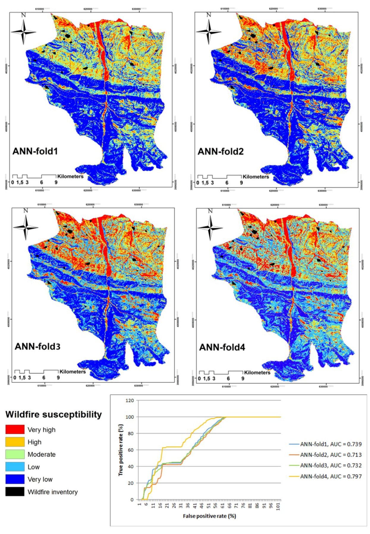
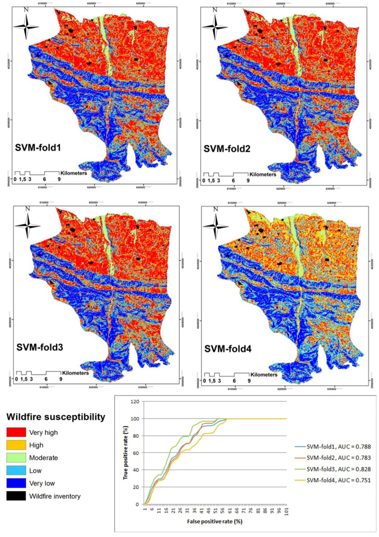
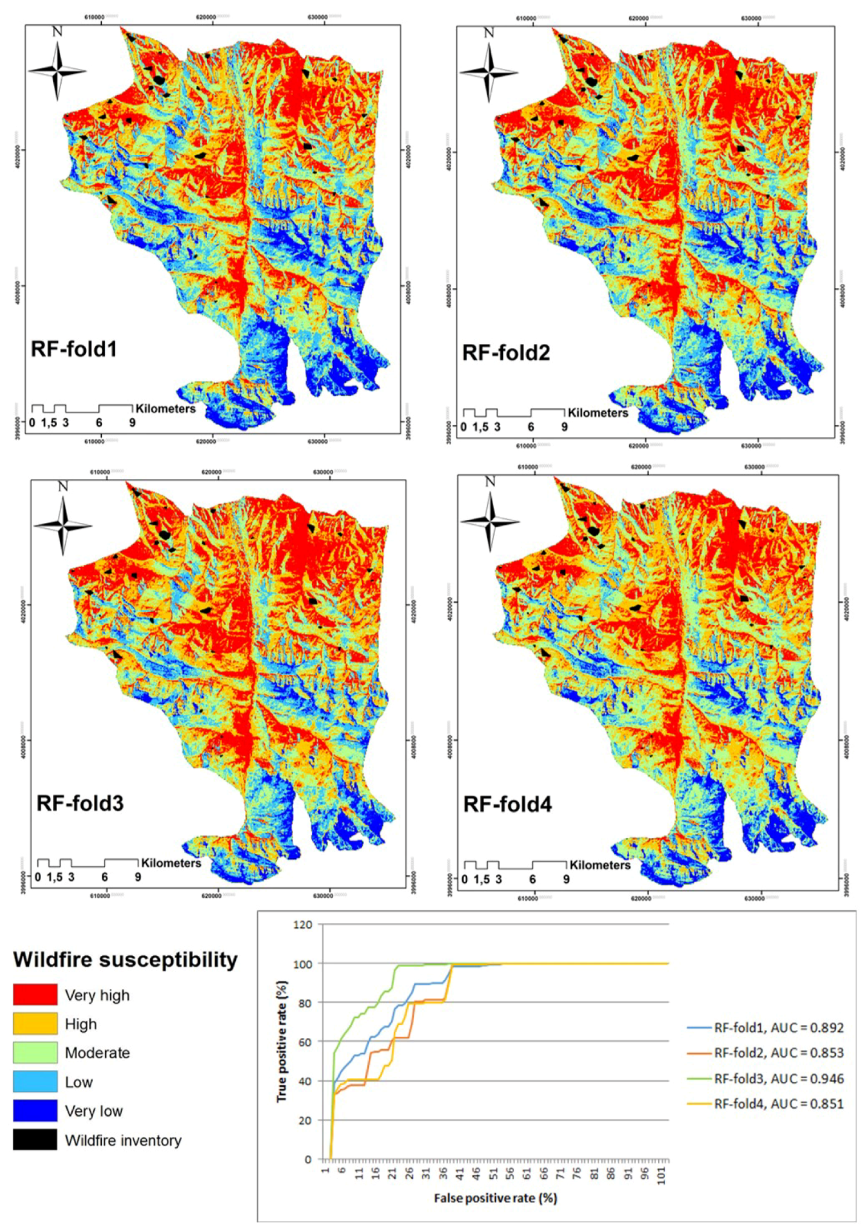
Table 7. The resulting accuracy of each fold and the CV values.
MLAUC-Fold1AUC-Fold2AUC-Fold3AUC-Fold4Cross-Validation (CV)
ANN0.740.710.730.790.74
SVM0.780.780.820.750.79
RF0.890.850.940.850.88

