
Point Cloud Based Mapping of Understory Shrub Fuel Distribution, Estimation of Fuel Consumption and Relationship to Pyrolysis Gas Emissions on Experimental Prescribed Burns †


 , , , , ,
  ,
,
Abstract
:1. Introduction
2. Methods
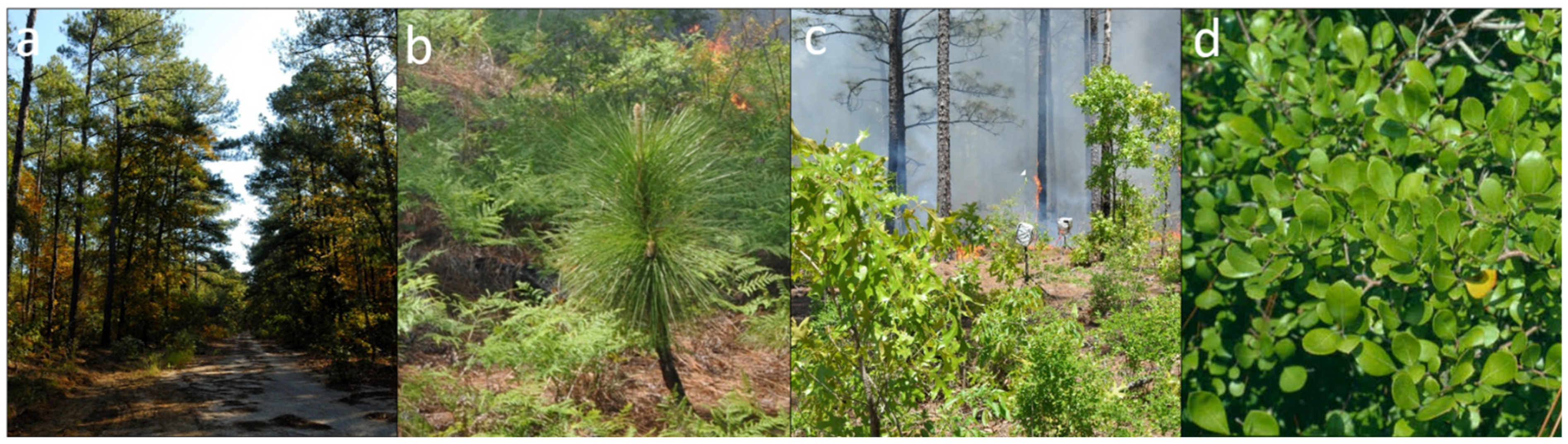
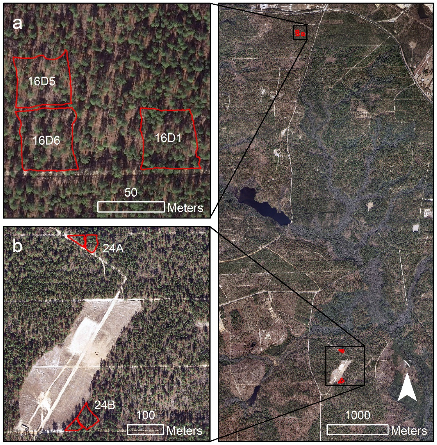
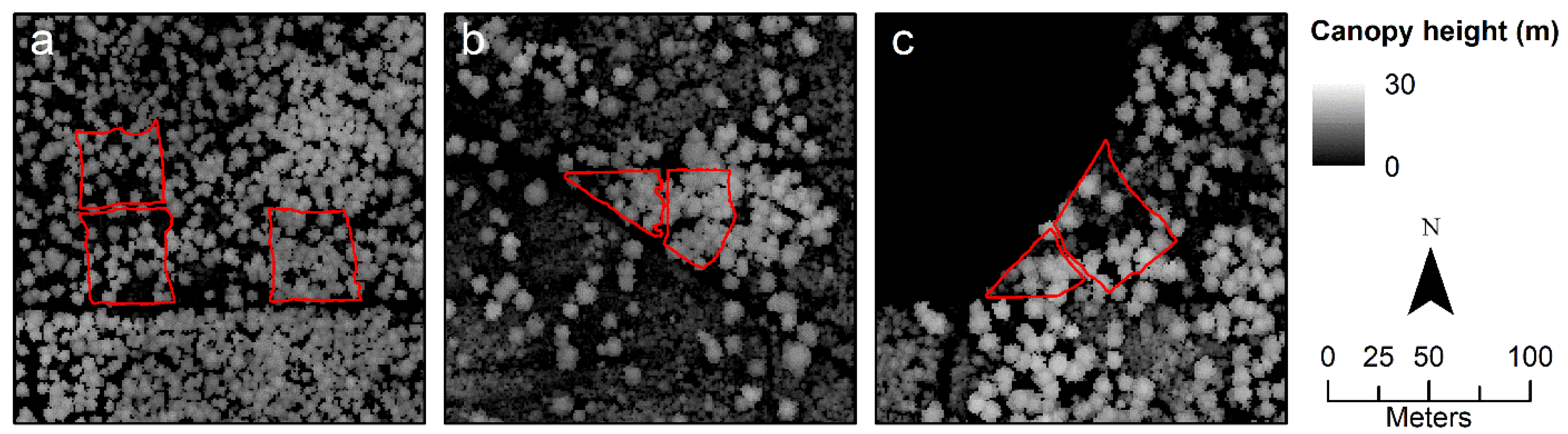
2.1. Study Area
2.2. In Situ Data Collection and Preparation
2.2.1. Airborne Laser Scanning
2.2.2. Terrestrial Laser Scanning
2.2.3. Unmanned Aerial Vehicle Imagery
2.2.4. Field Data
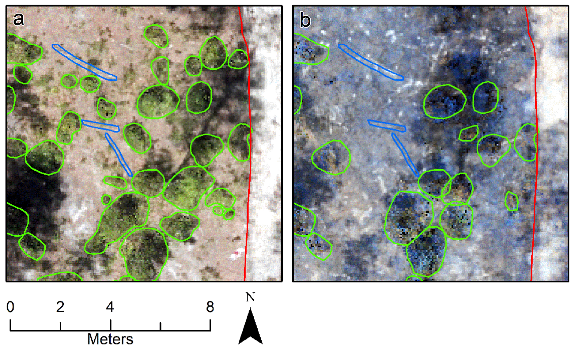
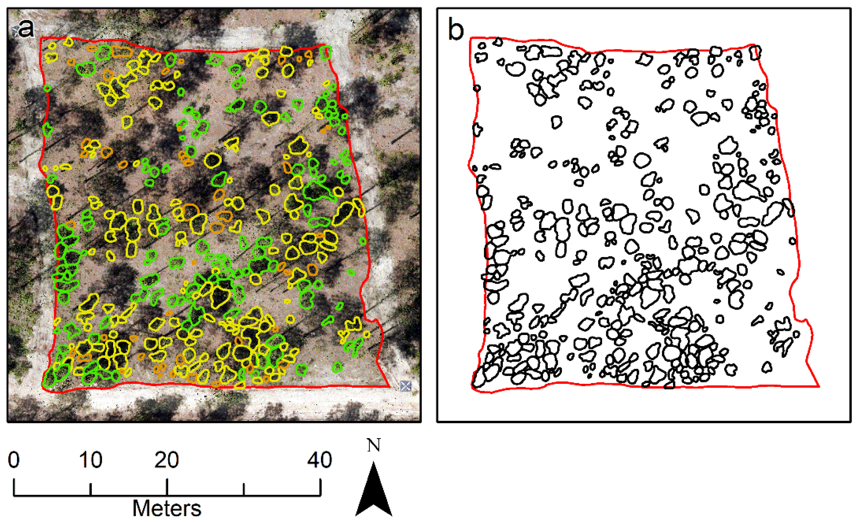
2.3. Digitization of Fuel Sources
2.3.1. Digitization
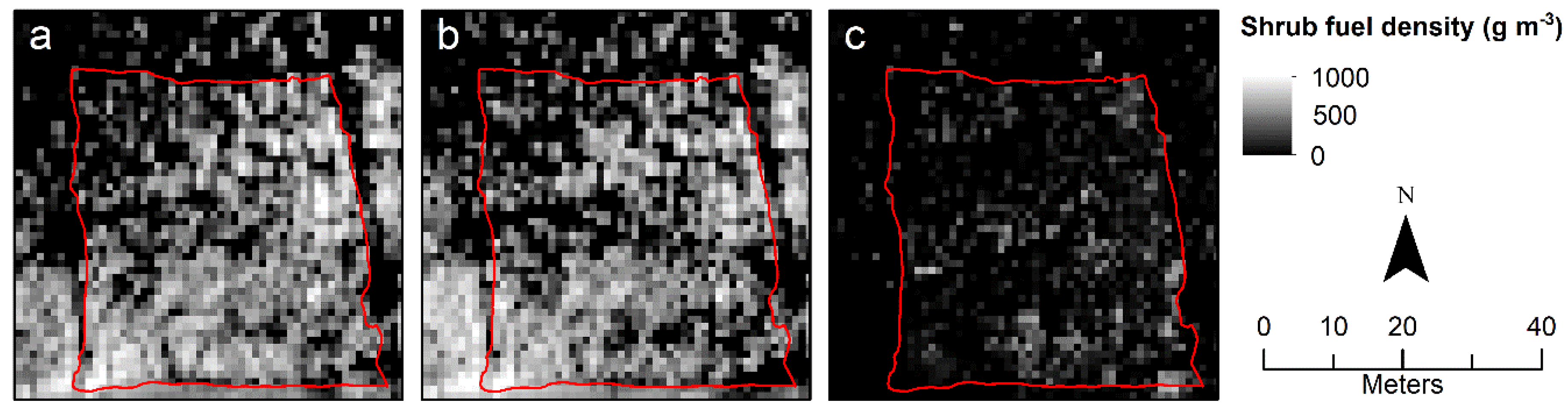
2.3.2. Rasterization
2.4. Ground Truth Measurements
2.5. Fourier Transform Infrared (FTIR) Spectroscopy Gas Analysis
2.6. Statistical Analysis
2.6.1. Tree Crowns vs. Sparkleberry Clumps Distribution
2.6.2. Ground Truth Measurements
2.6.3. Fuel Density/Consumption Estimates
2.6.4. Effect of Fuel Consumption on Composition of Pyrolysis Gases
3. Results
3.1. Tree Crowns vs. Sparkleberry Clumps Distribution
3.2. Ground Truth Measurements
3.3. Shrub Fuel Loading Estimates
3.4. Relationship between Fuel Consumption and Pyrolysis Gas Composition
4. Discussion and Conclusions
4.1. Tree Crowns vs. Sparkleberry Clumps Distribution
4.2. Ground Truth Measurements
4.3. Fuel Density/Consumption Estimates
4.4. Relationship between Fuel Consumption and Pyrolysis Gas Composition
Author Contributions
Funding
Institutional Review Board Statement
Informed Consent Statement
Acknowledgments
Conflicts of Interest
References
- Scott, A.C.; Bowman, D.M.; Bond, W.J.; Pyne, S.J.; Alexander, M.E. Fire on Earth: An Introduction; John Wiley & Sons: Hoboken, NJ, USA, 2013. [Google Scholar]
- Hiers, J.K.; O’Brien, J.J.; Varner, J.M.; Butler, B.W.; Dickinson, M.; Furman, J.; Gallagher, M.; Godwin, D.; Goodrick, S.L.; Hood, S.M. Prescribed fire science: The case for a refined research agenda. Fire Ecol. 2020, 16, 11. [Google Scholar] [CrossRef]
- Pyne, S.J. The Pyrocene: How We Created an Age of Fire, and What Happens Next; University of California Press: Oakland, CA, USA, 2021. [Google Scholar]
- Crutzen, P.J.; Heidt, L.E.; Krasnec, J.P.; Pollock, W.H.; Seiler, W. Biomass burning as a source of atmospheric gases CO, H2, N2O, NO, CH3Cl and COS. Nature 1979, 282, 253–256. [Google Scholar] [CrossRef]
- Burling, I.; Yokelson, R.J.; Griffith, D.W.; Johnson, T.J.; Veres, P.; Roberts, J.; Warneke, C.; Urbanski, S.; Reardon, J.; Weise, D. Laboratory measurements of trace gas emissions from biomass burning of fuel types from the southeastern and southwestern United States. Atmos. Chem. Phys. 2010, 10, 11115–11130. [Google Scholar] [CrossRef]
- Eck, T.; Holben, B.; Reid, J.; O’neill, N.; Schafer, J.; Dubovik, O.; Smirnov, A.; Yamasoe, M.; Artaxo, P. High aerosol optical depth biomass burning events: A comparison of optical properties for different source regions. Geophys. Res. Lett. 2003, 30. [Google Scholar] [CrossRef]
- Yokelson, R.J.; Susott, R.; Ward, D.E.; Reardon, J.; Griffith, D.W. Emissions from smoldering combustion of biomass measured by open-path Fourier transform infrared spectroscopy. J. Geophys. Res. Atmos. 1997, 102, 18865–18877. [Google Scholar] [CrossRef]
- Radke, L.F.; Hegg, D.A.; Hobbs, P.V.; Nance, J.D.; Lyons, J.H.; Laursen, K.K.; Weiss, R.E.; Riggan, P.J.; Ward, D.E. Particulate and trace gas emissions from large biomass fire in North America. In Global Biomass Burning: Atmospheric, Climatic, and Biospheric Implications; Levine, J.S., Ed.; The MIT Press: Cambridge, MA, USA, 1991; pp. 209–216. [Google Scholar]
- Rein, G. Smouldering combustion phenomena in science and technology. Int. Rev. Chem. Eng. 2009, 1, 3–18. [Google Scholar]
- Collard, F.-X.; Blin, J. A review on pyrolysis of biomass constituents: Mechanisms and composition of the products obtained from the conversion of cellulose, hemicelluloses and lignin. Renew. Sustain. Energy Rev. 2014, 38, 594–608. [Google Scholar] [CrossRef]
- Akagi, S.; Yokelson, R.J.; Wiedinmyer, C.; Alvarado, M.; Reid, J.; Karl, T.; Crounse, J.; Wennberg, P. Emission factors for open and domestic biomass burning for use in atmospheric models. Atmos. Chem. Phys. 2011, 11, 4039–4072. [Google Scholar] [CrossRef]
- Yokelson, R.J.; Burling, I.; Gilman, J.; Warneke, C.; Stockwell, C.; De Gouw, J.; Akagi, S.; Urbanski, S.; Veres, P.; Roberts, J. Coupling field and laboratory measurements to estimate the emission factors of identified and unidentified trace gases for prescribed fires. Atmos. Chem. Phys. 2013, 13, 89–116. [Google Scholar] [CrossRef]
- Rein, G. Smouldering Fires and Natural Fuels. In Fire Phenomena and the Earth System: An Interdisciplinary Guide to Fire Science, 1st ed.; Belcher, C.M., Ed.; John Wiley & Sons: Oxford, UK, 2013; pp. 15–33. [Google Scholar]
- Bostrom, D.; Skoglund, N.; Grimm, A.; Boman, C.; Ohman, M.; Brostrom, M.; Backman, R. Ash transformation chemistry during combustion of biomass. Energy Fuels 2012, 26, 85–93. [Google Scholar] [CrossRef]
- Qu, Z.; Schmidt, F.M. In situ H2O and temperature detection close to burning biomass pellets using calibration-free wavelength modulation spectroscopy. Appl. Phys. B 2015, 119, 45–53. [Google Scholar] [CrossRef]
- Yokelson, R.J.; Griffith, D.W.; Ward, D.E. Open-path Fourier transform infrared studies of large-scale laboratory biomass fires. J. Geophys. Res. Atmos. 1996, 101, 21067–21080. [Google Scholar] [CrossRef]
- Scharko, N.K.; Oeck, A.M.; Tonkyn, R.G.; Baker, S.P.; Lincoln, E.N.; Chong, J.; Corcoran, B.M.; Burke, G.M.; Weise, D.R.; Myers, T.L. Identification of gas-phase pyrolysis products in a prescribed fire: First detections using infrared spectroscopy for naphthalene, methyl nitrite, allene, acrolein and acetaldehyde. Atmos. Meas. Tech. 2019, 12, 763–776. [Google Scholar] [CrossRef]
- Akagi, S.K.; Burling, I.R.; Mendoza, A.; Johnson, T.J.; Cameron, M.; Griffith, D.W.; Paton-Walsh, C.; Weise, D.R.; Reardon, J.; Yokelson, R.J. Field measurements of trace gases emitted by prescribed fires in southeastern US pine forests using an open-path FTIR system. Atmos. Chem. Phys. 2014, 14, 199–215. [Google Scholar] [CrossRef]
- Burling, I.; Yokelson, R.J.; Akagi, S.; Urbanski, S.; Wold, C.E.; Griffith, D.W.; Johnson, T.J.; Reardon, J.; Weise, D. Airborne and ground-based measurements of the trace gases and particles emitted by prescribed fires in the United States. Atmos. Chem. Phys. 2011, 11, 12197–12216. [Google Scholar] [CrossRef]
- Gilman, J.; Lerner, B.; Kuster, W.; Goldan, P.; Warneke, C.; Veres, P.; Roberts, J.; De Gouw, J.; Burling, I.; Yokelson, R. Biomass burning emissions and potential air quality impacts of volatile organic compounds and other trace gases from fuels common in the US. Atmos. Chem. Phys. 2015, 15, 13915–13938. [Google Scholar] [CrossRef]
- Andreae, M.O.; Merlet, P. Emission of trace gases and aerosols from biomass burning. Glob. Biogeochem. Cycles 2001, 15, 955–966. [Google Scholar] [CrossRef]
- Koss, A.R.; Sekimoto, K.; Gilman, J.B.; Selimovic, V.; Coggon, M.M.; Zarzana, K.J.; Yuan, B.; Lerner, B.M.; Brown, S.S.; Jimenez, J.L. Non-methane organic gas emissions from biomass burning: Identification, quantification, and emission factors from PTR-ToF during the FIREX 2016 laboratory experiment. Atmos. Chem. Phys. 2018, 18, 3299–3319. [Google Scholar] [CrossRef]
- Scharko, N.K.; Oeck, A.M.; Myers, T.L.; Tonkyn, R.G.; Banach, C.A.; Baker, S.P.; Lincoln, E.N.; Chong, J.; Corcoran, B.M.; Burke, G.M.; et al. Gas-phase pyrolysis products emitted by prescribed fires in pine forests with a shrub understory in the southeastern United States. Atmos. Chem. Phys. 2019, 19, 9681–9698. [Google Scholar] [CrossRef]
- Weise, D.R.; Fletcher, T.H.; Johnson, T.J.; Hao, W.; Dietenberger, M.; Princevac, M.; Butler, B.; McAllister, S.; O’Brien, J.; Loudermilk, L. A project to measure and model pyrolysis to improve prediction of prescribed fire behavior. In Advances in Forest Fire Research 2018; Viegas, D.X., Ed.; University of Coimbra: Coimbra, Portugal, 2018; pp. 308–318. [Google Scholar]
- Ottmar, R.D.; Sandberg, D.V.; Riccardi, C.L.; Prichard, S.J. An overview of the fuel characteristic classification system—quantifying, classifying, and creating fuelbeds for resource planning. Can. J. For. Res. 2007, 37, 2383–2393. [Google Scholar] [CrossRef]
- Boyer, W.D. Techniques and Methods of Measuring Understory Vegetation. Proceedings of a Symposium on Forest Fire Research at Tifton, Georgia; Southern Forest Experiment Station: Tifton, GA, USA, 1959.
- Hudak, A.T.; Kato, A.; Bright, B.C.; Loudermilk, E.L.; Hawley, C.; Restaino, J.C.; Ottmar, R.D.; Prata, G.A.; Cabo, C.; Prichard, S.J. Towards spatially explicit quantification of pre-and postfire fuels and fuel consumption from traditional and point cloud measurements. For. Sci. 2020, 66, 428–442. [Google Scholar] [CrossRef]
- Banach, C.A.; Bradley, A.M.; Tonkyn, R.G.; Williams, O.N.; Chong, J.; Weise, D.R.; Myers, T.L.; Johnson, T.J. Dynamic infrared gas analysis from longleaf pine fuel beds burned in a wind tunnel: Observation of phenol in pyrolysis and combustion phases. Atmos. Meas. Tech. 2021, 14, 2359–2376. [Google Scholar] [CrossRef]
- Christensen, N.L. Vegetation of the Southeastern Coastal Plain, in North American Terrestrial Vegetation. In Northern American Terrestrial Vegetation, 2nd ed.; Billings, M.G.B.W.D., Ed.; Cambridge University Press: New York, NY, USA, 2000. [Google Scholar]
- Jackson, J. Red-cockaded Woodpecker (Dryobates borealis), version 1.0. In Birds of the World; Poole, A.F., Gill, F.B., Eds.; Cornell Lab of Ornithology: Ithaca, NY, USA, 2020. [Google Scholar]
- Silva, C.A.; Hudak, A.T.; Vierling, L.A.; Loudermilk, E.L.; O’Brien, J.J.; Hiers, J.K.; Jack, S.B.; Gonzalez-Benecke, C.; Lee, H.; Falkowski, M.J. Imputation of individual longleaf pine (Pinus palustris Mill.) tree attributes from field and LiDAR data. Can. J. Remote Sens. 2016, 42, 554–573. [Google Scholar] [CrossRef]
- Hudak, A.T.; Bright, B.C.; Pokswinski, S.M.; Loudermilk, E.L.; O’Brien, J.J.; Hornsby, B.S.; Klauberg, C.; Silva, C.A. Mapping forest structure and composition from low-density LiDAR for informed forest, fuel, and fire management at Eglin Air Force Base, Florida, USA. Can. J. Remote Sens. 2016, 42, 411–427. [Google Scholar] [CrossRef]
- Hudak, A.T.; Evans, J.S.; Stuart Smith, A.M. LiDAR utility for natural resource managers. Remote Sens. 2009, 1, 934–951. [Google Scholar] [CrossRef]
- Ullman, S. The Interpretation of Visual Motion; Massachusetts Inst of Technology: Cambridge, MA, USA, 1979; Volume 203, pp. 405–426. [Google Scholar]
- Hillman, S.; Wallace, L.; Reinke, K.; Hally, B.; Jones, S.; Saldias, D.S. A method for validating the structural completeness of understory vegetation models captured with 3D remote sensing. Remote Sens. 2019, 11, 2118. [Google Scholar] [CrossRef]
- Mathews, B.J.; Strand, E.K.; Smith, A.M.; Hudak, A.T.; Dickinson, B.; Kremens, R.L. Laboratory experiments to estimate interception of infrared radiation by tree canopies. Int. J. Wildland Fire 2016, 25, 1009–1014. [Google Scholar] [CrossRef]
- R Core Team. R: A Language and Environment for Statistical Computing; R Foundation for Statistical Computing: Vienna, Austria, 2021. [Google Scholar]
- Weise, D.R.; Hao, W.M.; Baker, S.; Princevac, M.; Aminfar, A.-H.; Palarea-Albaladejo, J.; Ottmar, R.D.; Hudak, A.T.; Restaino, J.; O’Brien, J.J. Comparison of fire-produced gases from wind tunnel and small field experimental burns. Int. J. Wildland Fire 2022, 31, 409–434. [Google Scholar] [CrossRef]
- Griffith, D.W.T. MALT5 User Guide Version 5.5.9. Wollongong, NSW, Australia. 2016. Available online: https://software-ab.informatik.uni-tuebingen.de/download/malt/welcome.html (accessed on 15 July 2022).
- Sharpe, S.W.; Johnson, T.J.; Sams, R.L.; Chu, P.M.; Rhoderick, G.C.; Johnson, P.A. Gas-phase databases for quantitative infrared spectroscopy. Appl. Spectrosc. 2004, 58, 1452–1461. [Google Scholar] [CrossRef]
- Gordon, I.E.; Rothman, L.S.; Hill, C.; Kochanov, R.V.; Tan, Y.; Bernath, P.F.; Birk, M.; Boudon, V.; Campargue, A.; Chance, K. The HITRAN2016 molecular spectroscopic database. J. Quant. Spectrosc. Radiat. Transf. 2017, 203, 3–69. [Google Scholar] [CrossRef]
- USDA NRCS. The PLANTS Database. Available online: http://plants.usda.gov (accessed on 15 July 2022).
- NC State Extension. North Carolina Extension Gardener Plant Toolbox. Available online: https://plants.ces.ncsu.edu/ (accessed on 23 February 2022).
- De Winter, J.C. Using the Student’s t-test with extremely small sample sizes. Pract. Assess. Res. Eval. 2013, 18, 10. [Google Scholar]
- Aitchinson, J. The Statistical Analysis of Compositional Data. Monographs on Statistics and Applied Probability; Chapman and Halll: London, UK; New York, NY, USA, 1986. [Google Scholar]
- Weise, D.R.; Palarea-Albaladejo, J.; Johnson, T.J.; Jung, H. Analyzing wildland fire smoke emissions data using compositional data techniques. J. Geophys. Res. Atmos. 2020, 125, e2019JD032128. [Google Scholar] [CrossRef]
- Weise, D.R.; Fletcher, T.H.; Safdari, M.-S.; Amini, E.; Palarea-Albaladejo, J. Application of compositional data analysis to determine the effects of heating mode, moisture status and plant species on pyrolysates. Int. J. Wildland Fire 2021, 31, 24–45. [Google Scholar] [CrossRef]
- Weise, D.R.; Jung, H.; Palarea-Albaladejo, J.; Cocker, D.R. Compositional data analysis of smoke emissions from debris piles with low-density polyethylene. J. Air Waste Manag. Assoc. 2020, 70, 834–845. [Google Scholar] [CrossRef]
- Egozcue, J.J.; Pawlowsky-Glahn, V.; Mateu-Figueras, G.; Barcelo-Vidal, C. Isometric logratio transformations for compositional data analysis. Math. Geol. 2003, 35, 279–300. [Google Scholar] [CrossRef]
- Palarea-Albaladejo, J.; Martín-Fernández, J.A.; Buccianti, A. Compositional methods for estimating elemental concentrations below the limit of detection in practice using R. J. Geochem. Explor. 2014, 141, 71–77. [Google Scholar] [CrossRef]
- Palarea-Albaladejo, J.; Martín-Fernández, J.A. zCompositions—R package for multivariate imputation of left-censored data under a compositional approach. Chemom. Intell. Lab. Syst. 2015, 143, 85–96. [Google Scholar] [CrossRef]
- McNaught, A.D.; Wilkinson, A. Compendium of Chemical Terminology; Blackwell Science: Oxford, UK, 1997; Volume 1669. [Google Scholar]
- Oksanen, J.; Blanchet, F.G.; Friendly, M.; Kindt, R.; Wagner, H.H. Vegan: Community Ecology Package. R Package Version 2.5-7; R Welthandelsplatz 1: Vienna, Austria, 2020. [Google Scholar]
- Anderson, M.J. A new method for non-parametric multivariate analysis of variance. Austral Ecol. 2001, 26, 32–46. [Google Scholar]
- Van den Boogaart, K.G.; Tolosana-Delgado, R. Analyzing Compositional Data with R; Springer: Berlin/Heidelberg, Germany, 2013; Volume 122. [Google Scholar]
- Anderson, M.J. Permutational Multivariate Analysis of Variance (PERMANOVA). In Wiley StatsRef: Statistics Reference Online; John Wiley & Sons: Hoboken, NJ, USA, 2014; pp. 1–15. [Google Scholar]
- Benjamini, Y.; Hochberg, Y. Controlling the false discovery rate: A practical and powerful approach to multiple testing. J. R. Stat. Soc. Ser. B 1995, 57, 289–300. [Google Scholar] [CrossRef]
- Wenk, E.S.; Wang, G.G.; Walker, J.L. Within-stand variation in understorey vegetation affects fire behaviour in longleaf pine xeric sandhills. Int. J. Wildland Fire 2011, 20, 866–875. [Google Scholar] [CrossRef]
- Lozano, J.S. An Investigation of Surface and Crown Fire Dynamics in Shrub Fuels; University of California: Riverside, CA, USA, 2011. [Google Scholar]
- Tachajapong, W.; Lozano, J.; Mahalingam, S.; Weise, D.R. Experimental modelling of crown fire initiation in open and closed shrubland systems. Int. J. Wildland Fire 2014, 23, 451–462. [Google Scholar] [CrossRef]
- Marino, E.; Guijarro, M.; Madrigal, J.; Hernando, C.; Diez, C. Assessing fire propagation empirical models in shrub fuel complexes using wind tunnel data. WIT Trans. Ecol. Environ. 2008, 119, 121–130. [Google Scholar]
- Cobian-Iñiguez, J.; Aminfar, A.; Weise, D.R.; Princevac, M. On the Use of Semi-empirical Flame Models for Spreading Chaparral Crown Fire. Front. Mech. Eng. 2019, 5, 50. [Google Scholar] [CrossRef]
- Keane, R.E.; Gray, K.; Bacciu, V. Spatial Variability of Wildland Fuel Characteristics in Northern Rocky Mountain Ecosystems; Research Paper RMRS-RP-98; USDA Forest Service, Rocky Mountain Research Station: Fort Collins, CO, USA, 2012; Volume 98, 56p.
- Parresol, B.R.; Blake, J.I.; Thompson, A.J. Effects of overstory composition and prescribed fire on fuel loading across a heterogeneous managed landscape in the southeastern USA. For. Ecol. Manag. 2012, 273, 29–42. [Google Scholar] [CrossRef]
- Skowronski, N.; Clark, K.; Nelson, R.; Hom, J.; Patterson, M. Remotely sensed measurements of forest structure and fuel loads in the Pinelands of New Jersey. Remote Sens. Environ. 2007, 108, 123–129. [Google Scholar] [CrossRef]
- Ottmar, R.D.; Hudak, A.T.; Prichard, S.J.; Wright, C.S.; Restaino, J.C.; Kennedy, M.C.; Vihnanek, R.E. Pre-fire and post-fire surface fuel and cover measurements collected in the south-eastern United States for model evaluation and development–RxCADRE 2008, 2011 and 2012. Int. J. Wildland Fire 2015, 25, 10–24. [Google Scholar] [CrossRef]
- Hudak, A.T.; Dickinson, M.B.; Bright, B.C.; Kremens, R.L.; Loudermilk, E.L.; O’Brien, J.J.; Hornsby, B.S.; Ottmar, R.D. Measurements relating fire radiative energy density and surface fuel consumption–RxCADRE 2011 and 2012. Int. J. Wildland Fire 2015, 25, 25–37. [Google Scholar] [CrossRef]
- Demirbas, A.; Arin, G. An overview of biomass pyrolysis. Energy Sour. 2002, 24, 471–482. [Google Scholar] [CrossRef]
- Kan, T.; Strezov, V.; Evans, T.J. Lignocellulosic biomass pyrolysis: A review of product properties and effects of pyrolysis parameters. Renew. Sustain. Energy Rev. 2016, 57, 1126–1140. [Google Scholar] [CrossRef]
- Hajaligol, M.R.; Howard, J.B.; Longwell, J.P.; Peters, W.A. Product compositions and kinetics for rapid pyrolysis of cellulose. Ind. Eng. Chem. Process Des. Dev. 1982, 21, 457–465. [Google Scholar] [CrossRef]
- Butler, B.; Cohen, J.; Latham, D.; Schuette, R.; Sopko, P.; Shannon, K.; Jimenez, D.; Bradshaw, L. Measurements of radiant emissive power and temperatures in crown fires. Can. J. For. Res. 2004, 34, 1577–1587. [Google Scholar] [CrossRef]


| Burn Unit | Plot Area (m2) | Tree Crown Area (m2) | Tree Crown Area/Plot Area | Sparkleberry Area (m2) | Sparkleberry Area/Plot Area | Overlap Area (m2) | Overlap Area/Sparkleberry Area |
|---|---|---|---|---|---|---|---|
| 16D1 | 1796.2 | 1218.2 | 0.67 | 416.2 | 0.23 | 303.1 | 0.72 |
| 16D5 | 1478.2 | 674.1 | 0.45 | 348.7 | 0.23 | 160.7 | 0.46 |
| 16D6 | 1860.5 | 754.3 | 0.40 | 245.0 | 0.13 | 90.5 | 0.37 |
| 24A Main | 1342.5 | 1060.9 | 0.77 | 282.6 | 0.21 | 184.5 | 0.81 |
| 24A Triangle | 873.2 | 574.2 | 0.50 | 227.6 | 0.26 | 159.9 | 0.71 |
| 24B Main | 2242.0 | 1246.8 | 0.41 | 332.1 | 0.15 | 371.4 | 0.67 |
| 24B Triangle | 838.7 | 586.6 | 0.37 | 56.3 | 0.07 | 58.4 | 0.75 |
| Burn Unit | Digitized | Ground Truth |
|---|---|---|
| 24A Main | 0.137 | 0.211 |
| 24A Triangle | 0.183 | 0.261 |
| 24B Main | 0.166 | 0.148 |
| 24B Triangle | 0.070 | 0.067 |
| Burn Unit | Preburn | Postburn | ||||||
|---|---|---|---|---|---|---|---|---|
| DIN | GIN | DOUT | GOUT | DIN | GIN | DOUT | GOUT | |
| 16D1 | 547 | 398 | 487 | 360 | ||||
| 16D5 | 700 | 488 | 563 | 350 | ||||
| 16D6 | 589 | 326 | 458 | 236 | ||||
| 24A Main | 492 | 510 | 435 | 496 | 485 | 421 | 438 | 428 |
| 24A Triangle | 585 | 550 | 521 | 496 | 569 | 514 | 495 | 521 |
| 24B Main | 256 | 183 | 136 | 118 | 150 | 138 | 87 | 84 |
| 24B Triangle | 211 | 135 | 254 | 123 | 198 | 277 | 232 | 253 |
| Model | Intercept | Slope | Pr > F | Adj. R2 | Estimated Fuel Loading | ||
|---|---|---|---|---|---|---|---|
| 16D1 | 16D5 | 16D6 | |||||
| InsidePreburn | −110.54 | 1.18 ** | 0.009 | 0.97 | 533.8 | 714.9 | 584.0 |
| OutsidePreburn | 19.16 | 0.95 ** | 0.003 | 0.99 | 395.5 | 481.2 | 327.4 |
| InsidePostBurn | −51.73 | 1.03 * | 0.017 | 0.95 | 448.6 | 525.7 | 418.7 |
| OutsidePostBurn | 1.70 | 1.02 ** | 0.004 | 0.99 | 370.1 | 359.3 | 243.2 |
| Burn Unit | |||||
|---|---|---|---|---|---|
| Gas | 24B Main | 24A Triangle | 16D5 | 16D6 | 16D1 |
| H2O | 243,741 1 | 19,839 | 10,073 | 8916 | 15,193 |
| CO2 | 13,637 | 65,899 | 67,508 | 53,715 | 38,852 |
| CO | 2928 | 15,886 | 11,207 | 10,664 | 6546 |
| CH4 | 306 | 1591 | 1261 | 1269 | 553 |
| C2H2 | 80 | 623 | 593 | 527 | 234 |
| C2H4 | 185 | 1013 | 822 | 657 | 340 |
| C2H6 | 24.6 | 100.8 | 55.9 | 52.0 | 28.0 |
| Allene | 2.4 | 18.2 | 15.7 | 12.4 | 6.1 |
| C3H6 | 27.3 | 181.3 | 113.7 | 85.0 | 48.8 |
| C4H6 | 4.2 | 72.6 | 41.9 | 26.8 | 15.8 |
| Isobutene | 0.6 | 14.6 | 8.7 | 3.8 | 2.7 |
| Isoprene | 0.7 | 41.5 | 12.2 | 3.5 | 2.8 |
| CH3OH | 56.5 | 91.4 | 42.7 | 33.3 | 21.7 |
| CH3COOH | 61.1 | 27.5 | 16.7 | 6.3 | 11.8 |
| HCOOH | 5.1 | 9.7 | 8.3 | 3.1 | 5.0 |
| CH3CHO | 47.3 | 181.7 | 94.3 | 70.2 | 43.5 |
| Acrolein | 25.5 | 75.8 | 37.7 | 26.3 | 18.2 |
| Acetone | 21.6 | 48.7 | 25.0 | 19.1 | 13.3 |
| HCHO | 45.6 | 64.4 | 17.7 | 6.3 | 10.2 |
| Furan | 5.4 | 17.4 | 6.4 | 6.2 | 3.7 |
| Furfural | 13.1 | 21.9 | 7.5 | 8.0 | 5.5 |
| Naphthalene | 1.0 | 4.4 | 6.5 | 12.2 | 7.4 |
| Methyl nitrite | 6.1 | 10.5 | 3.4 | 4.3 | 8.1 |
| HCN | 20.1 | 92.7 | 103.4 | 86.3 | 51.2 |
| HONO | 4.6 | 1.8 | 0.6 | 0.8 | 1.7 |
| Predictor | F-Statistic | Pr > F | R2 |
|---|---|---|---|
| Digitized Inside | 0.30 | 0.83 | 0.09 |
| Ground truth Inside | 1.58 | 0.29 | 0.35 |
| Digitized Outside | 0.51 | 0.70 | 0.14 |
| Ground truth Outside | 0.32 | 0.83 | 0.10 |
Publisher’s Note: MDPI stays neutral with regard to jurisdictional claims in published maps and institutional affiliations. |
© 2022 by the authors. Licensee MDPI, Basel, Switzerland. This article is an open access article distributed under the terms and conditions of the Creative Commons Attribution (CC BY) license (https://creativecommons.org/licenses/by/4.0/).
Share and Cite
Herzog, M.M.; Hudak, A.T.; Weise, D.R.; Bradley, A.M.; Tonkyn, R.G.; Banach, C.A.; Myers, T.L.; Bright, B.C.; Batchelor, J.L.; Kato, A.; et al. Point Cloud Based Mapping of Understory Shrub Fuel Distribution, Estimation of Fuel Consumption and Relationship to Pyrolysis Gas Emissions on Experimental Prescribed Burns. Fire 2022, 5, 118. https://doi.org/10.3390/fire5040118
Herzog MM, Hudak AT, Weise DR, Bradley AM, Tonkyn RG, Banach CA, Myers TL, Bright BC, Batchelor JL, Kato A, et al. Point Cloud Based Mapping of Understory Shrub Fuel Distribution, Estimation of Fuel Consumption and Relationship to Pyrolysis Gas Emissions on Experimental Prescribed Burns. Fire. 2022; 5(4):118. https://doi.org/10.3390/fire5040118
Chicago/Turabian StyleHerzog, Molly M., Andrew T. Hudak, David R. Weise, Ashley M. Bradley, Russell G. Tonkyn, Catherine A. Banach, Tanya L. Myers, Benjamin C. Bright, Jonathan L. Batchelor, Akira Kato, and et al. 2022. "Point Cloud Based Mapping of Understory Shrub Fuel Distribution, Estimation of Fuel Consumption and Relationship to Pyrolysis Gas Emissions on Experimental Prescribed Burns" Fire 5, no. 4: 118. https://doi.org/10.3390/fire5040118