
Cardiovascular Circulatory System and Left Carotid Model: A Fractional Approach to Disease Modeling

 , , , , ,
  and
and 
Abstract
:1. Introduction
2. Cardiovascular System
2.1. Anatomy and Physiology of the CVS
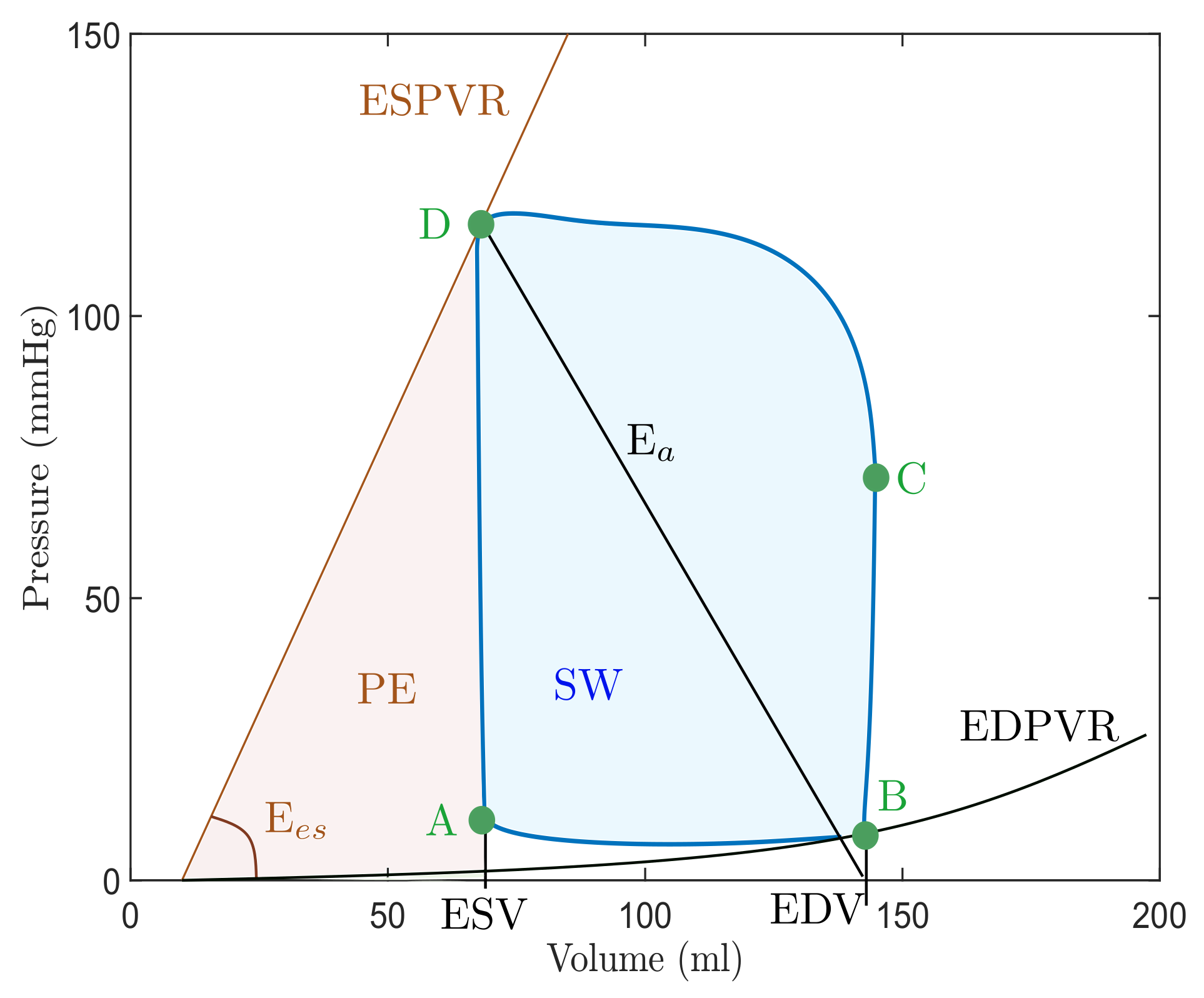
2.2. Cardiac Cycle and Pressure–Volume Loops
- (1)
- Passive filling (referred to as A-B);
- (2)
- Isovolumetric contraction (denoted as B-C);
- (3)
- Ejection (C-D);
- (4)
- Isovolumetric relaxation (D-A) [46].


| Abbreviation | Parameter | Meaning |
|---|---|---|
| EDV | End-diastolic volume | Left ventricular volume in diastole. |
| ESV | End-systolic volume | Left ventricular volume in systole. |
| ESPVR | End-systolic PV relationship | Maximal pressure of left ventricle. |
| EDPVR | End-diastolic PV relationship | Left ventricular pressure in diastole. |
| E | End-systolic elastance | Peak chamber elastance during a beat. |
| E | Effective arterial elastance | Relates EDP and EDV to ESV. |
| SV | Stroke volume | The difference between ESV and EDV. |
| SW | Stroke work | The area within the loop. |
| PE | Potential energy | The area within the loop and ESPVR. |
| PVA | Pressure–volume area | Sum of SW and potential energy PE. |
| ME | Mechanical efficiency | The ratio between SW and PVA. |
2.3. Valve Pathologies
3. Description of the CVS Model
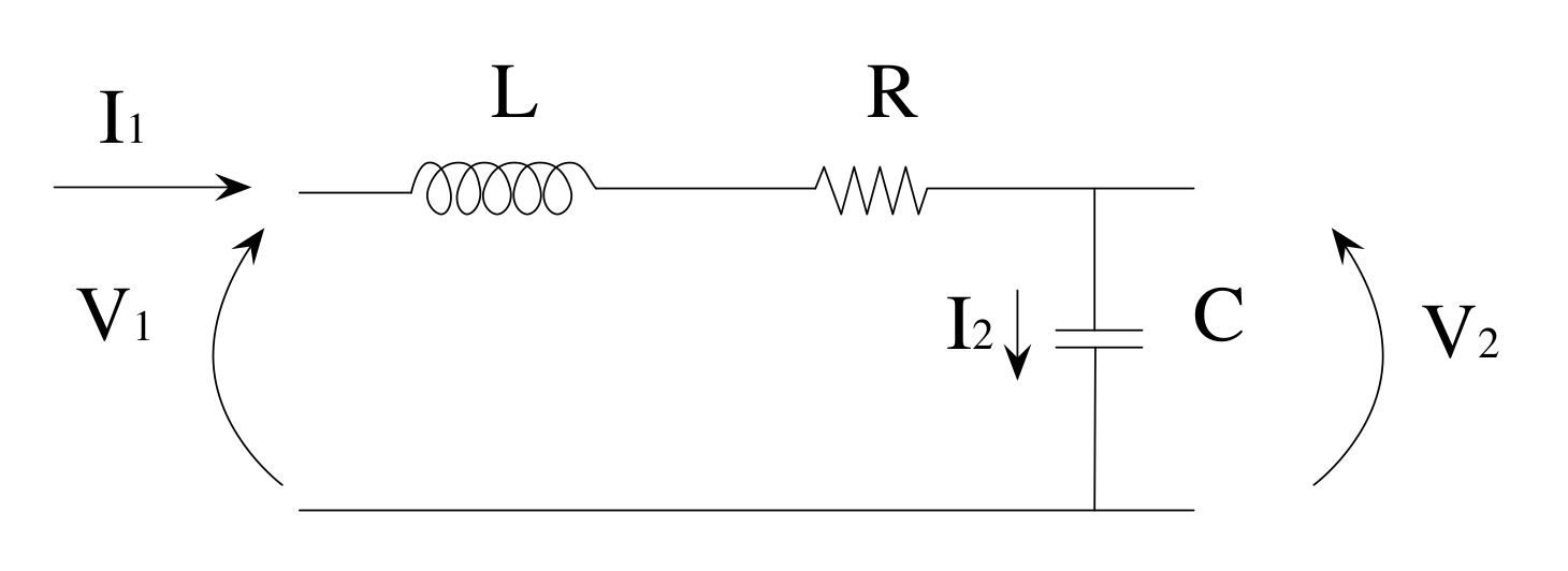
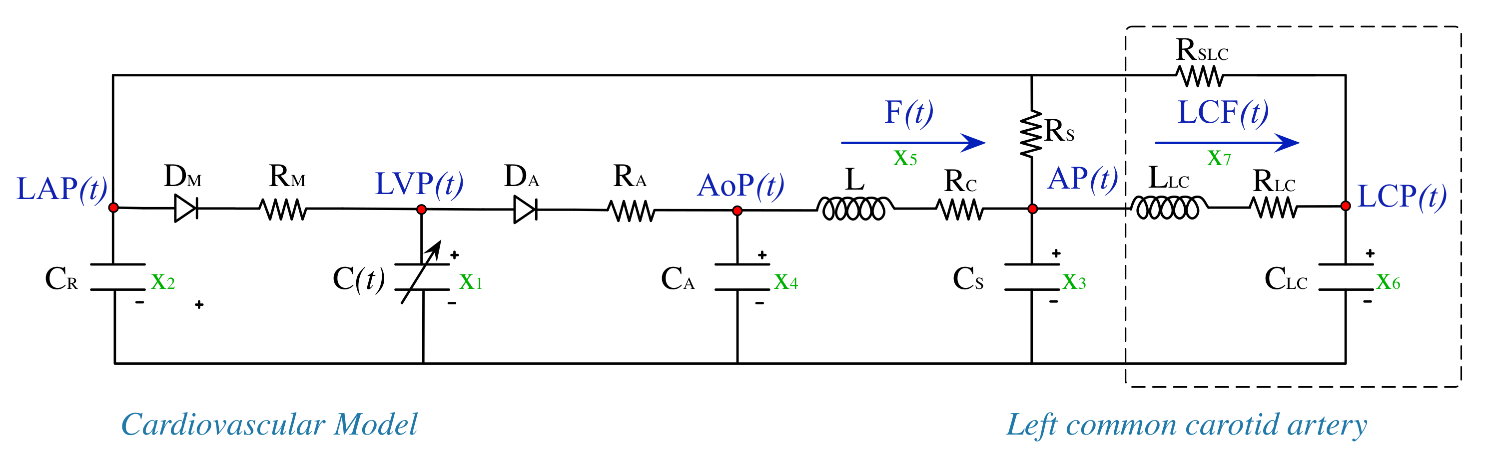
3.1. Electrical Equivalences
3.2. Model
| Variable | Abbreviation | Clinical Meaning (Unit) |
|---|---|---|
| (t) | LVP(t) | Left ventricular pressure (mmHg). |
| (t) | LAP(t) | Left atrial pressure (mmHg). |
| (t) | AP(t) | Descending aorta pressure (mmHg). |
| (t) | AoP(t) | Ascending aorta pressure (mmHg). |
| (t) | F(t) | Total flow (mL/s). |
| (t) | LCP(t) | Left common carotid artery pressure (mmHg). |
| (t) | LCF(t) | Carotid artery flow rate (mL/s). |
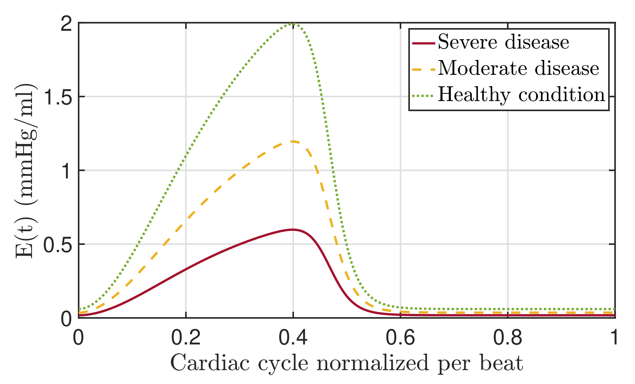
3.3. Elastance
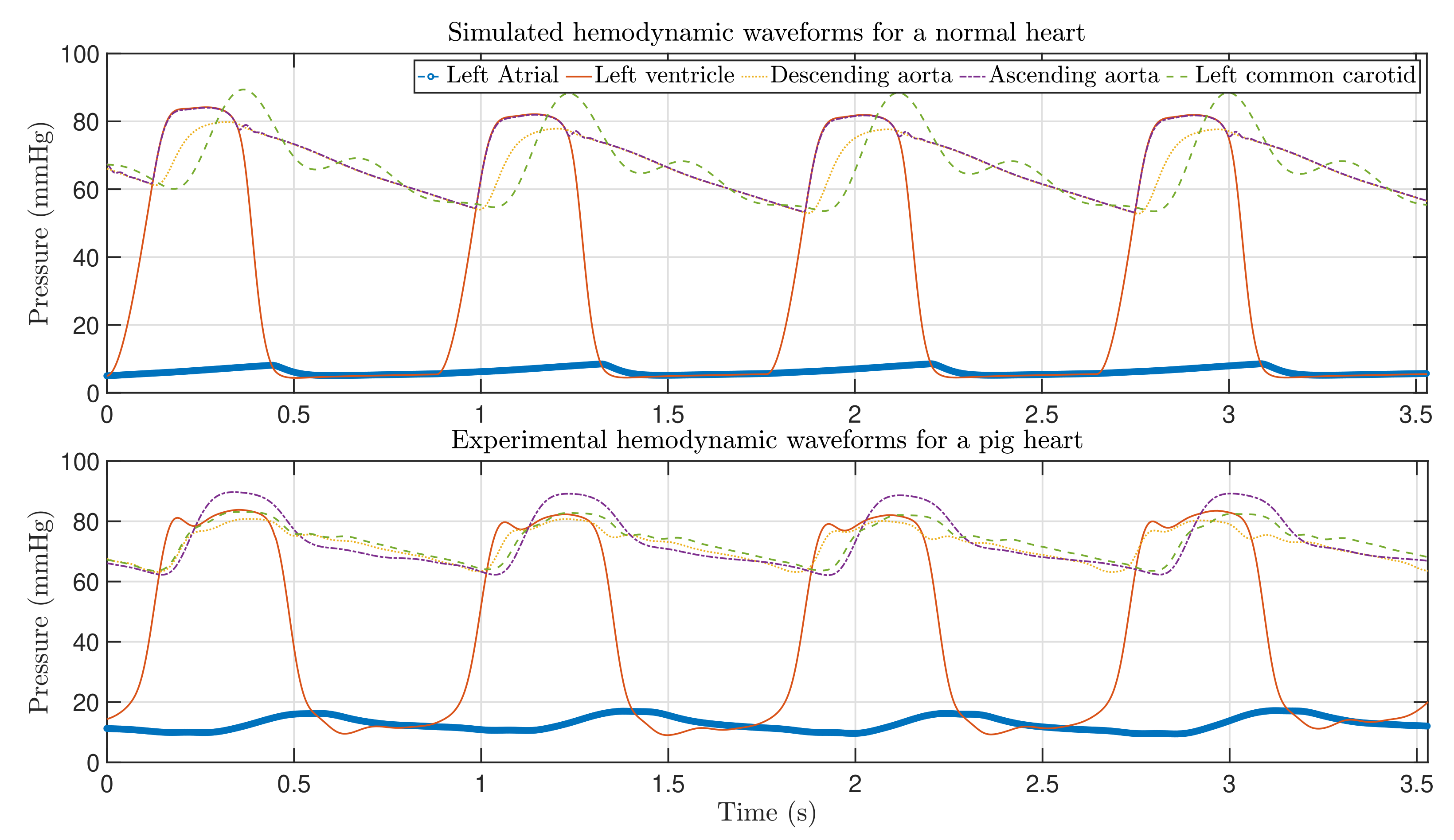
4. Validation of the CVS Model
4.1. Clinical Parameters and Experimental Waveforms
| Parameter | Value | Physiological Meaning |
|---|---|---|
| Resistors | ||
| R | 1 | Total peripheral resistance |
| R | 10 | Left common carotid peripheral resistance |
| R | Mitral valve resistance | |
| R | Aortic valve resistance | |
| R | Characteristic resistance | |
| R | 10 | Left common carotid resistance |
| Capacitors | ||
| C | Left atrial compliance | |
| C | Systemic compliance | |
| C | Aortic compliance | |
| C | Left common carotid | |
| Inductors | ||
| L | Inertia of blood in aorta | |
| L | Inertia of blood in left common carotid | |
| Left ventricle | ||
| 2 | Maximum volume in diastole | |
| Minimum volume in diastole | ||
| 10 | Reference volume at zero pressure (mL) | |
| HR | 75 | Heart rate (bpm) |
| Elastance | ||
| A | Shape parameter | |
| B | Shape parameter | |
| C | Amplitude | |
| Ascending slope of the LV relaxation time | ||
| Descending slope of the LV relaxation time |
| Data from | Heart Rate Pressure (mmHg) | Systolic Arterial Pressure (mmHg) | Diastolic Arterial Pressure (mmHg) | Mean Arterial Pressure (L/s) | Cardiac Output CO (mL/beat) | ||
| Literature | 50–90 | 90–140 | 60–90 | 70–105 | 4–8 | ||
| Model | 68 | 112 | 77 | 92 | |||
| Experiments | 67–70 | 89 | 62 | 68 | |||
| Data from | Stroke Volume SV (mmHg) | Systolic LVP (mmHg) | Diastolic LVP (mL) | Max LVV (mL) | Min LVV (mmHg) | Systolic LAP (mmHg) | Diastolic LVV (mmHg) |
| Literature | 60–100 | 100–140 | 4–15 | 77–195 | 19–72 | ∼12 | ∼12 |
| Model | 78.71 | 117 | 7 | 137 | 67 | 12 | 7 |
| Experiments | 46.83 | 82 | 9 | — | — | 16 | 10.5 |
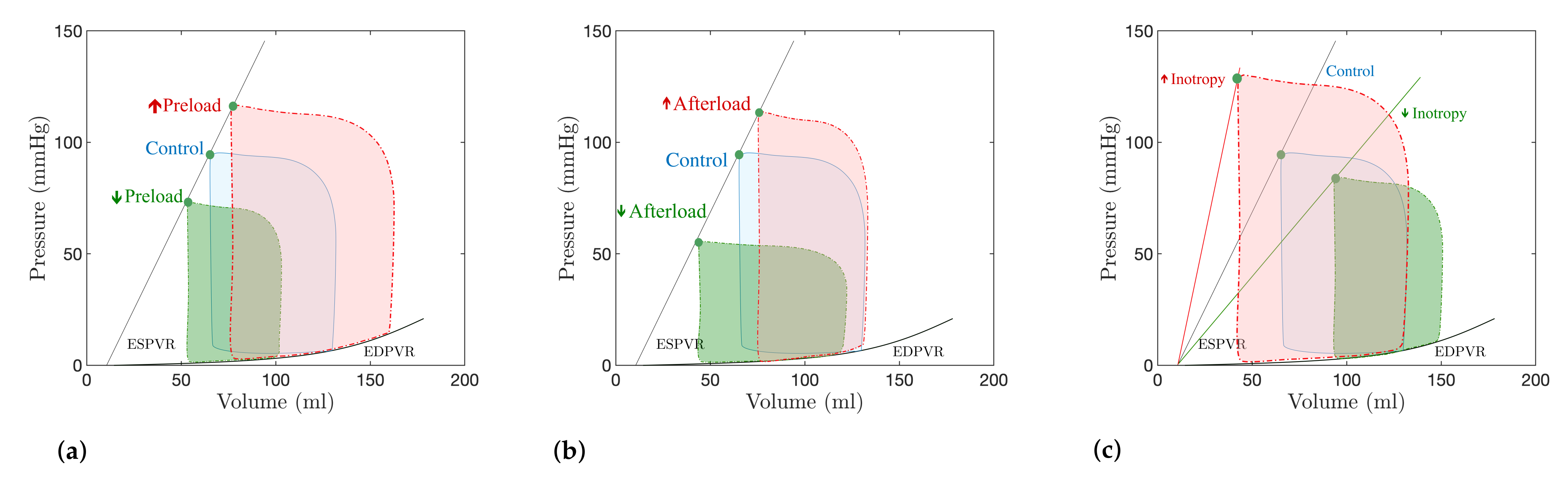
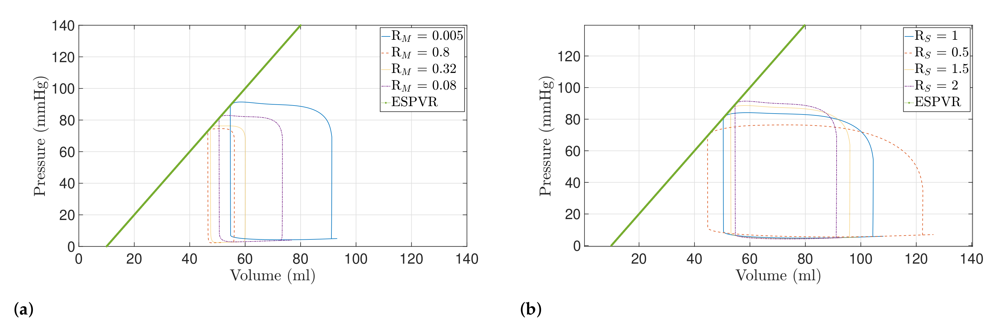
4.2. Preload and Afterload Dynamics
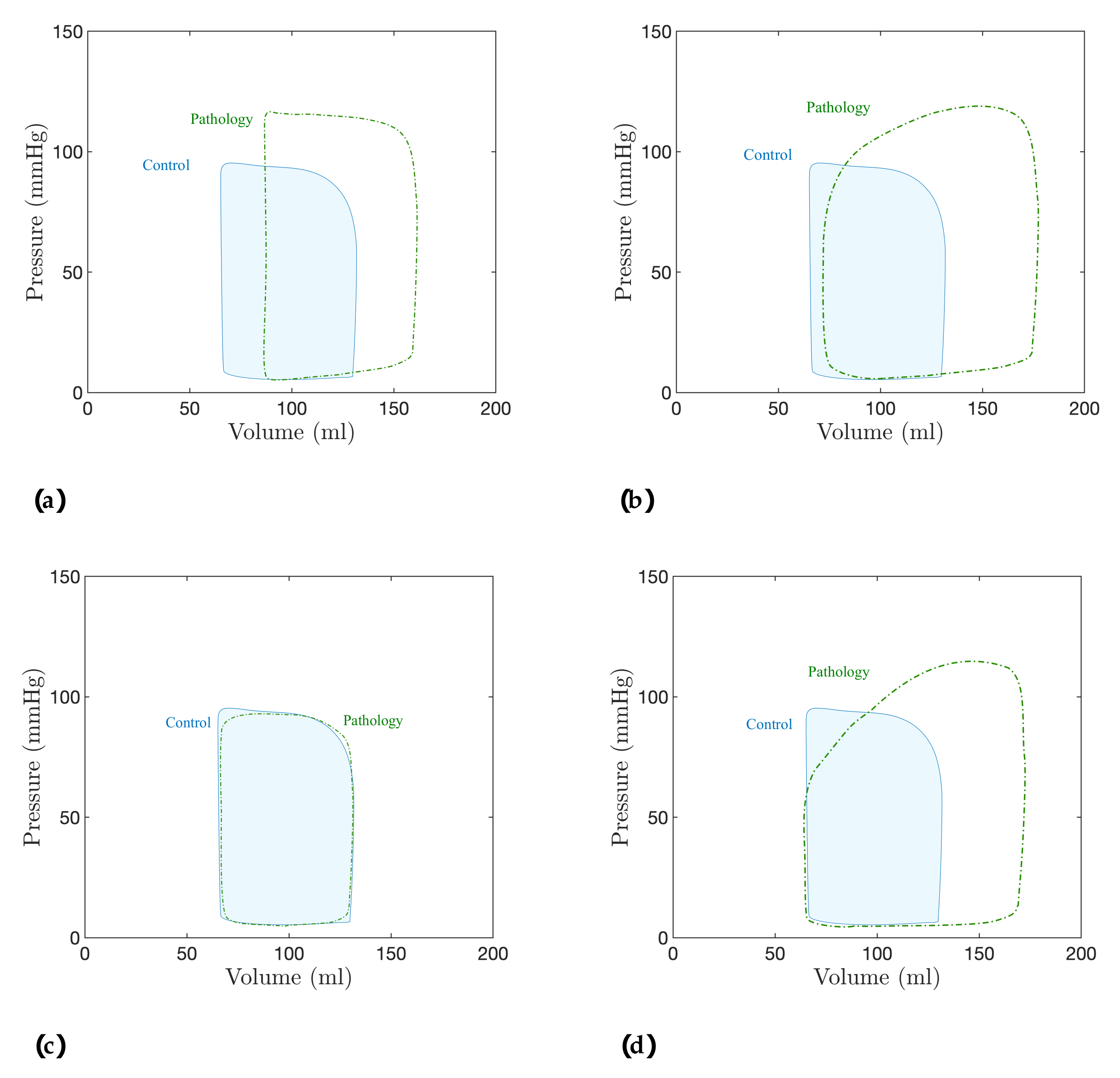
5. Discussion: Modeling of Pathologies
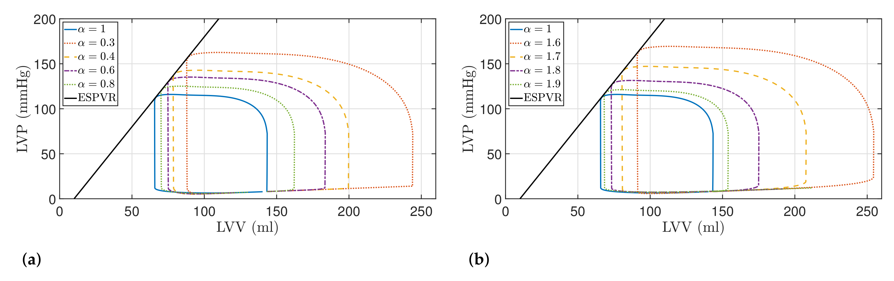
5.1. Fractional-Order Model
5.2. Results
| Model Order | SV (mL) | SW (J/beat) | PE (J/beat) | PVA (J/beat) | ME (%) | |
|---|---|---|---|---|---|---|
| Healthy | ||||||
| 92.01 (18.43%) | 1.34 (29.12%) | 0.45 (17.27%) | 1.79 (25.91%) | 74.78 (2.54%) | ||
| 108.62 (39.81%) | 1.70 (64.14%) | 0.52 (37.25%) | 2.23 (56.86%) | 76.30 (4.63%) | ||
| 121.08 (55.85%) | 2.00 (92.73%) | 0.59 (53.21%) | 2.59 (82.03%) | 77.21 (5.87%) | ||
| 156.01 (100.81%) | 2.89 (178.77%) | 0.76 (98.46%) | 3.66 (157.03%) | 79.09 (8.45%) | ||
| 85.57 (10.14%) | 1.19 (15.22%) | 0.42 (9.51%) | 1.62 (13.67%) | 73.91 (1.35%) | ||
| 102.88 (32.42%) | 1.54 (48.52%) | 0.49 (29.06%) | 2.04 (43.23%) | 75.60 (3.67%) | ||
| 127.03 (63.50%) | 2.14 (106.18%) | 0.62 (61.81%) | 2.76 (94.17%) | 77.43 (6.18%) | ||
| 163.27 (110.15%) | 3.13 (201.88%) | 0.83 (115.01%) | 3.96 (178.36%) | 79.08 (8.44%) | ||
6. Conclusions
Supplementary Materials
Author Contributions
Funding
Institutional Review Board Statement
Informed Consent Statement
Data Availability Statement
Acknowledgments
Conflicts of Interest
Abbreviations
| MDPI | Multidisciplinary Digital Publishing Institute |
| CVD | Cardiovascular disease |
| WHO | World Health Organization |
| CVS | Cardiovascular system |
| PV | Pressure-volume |
| EDV | End-diastolic volume |
| ESV | End-systolic volume |
| ESPVR | End-systolic PV relationship |
| EDPVR | End-diastolic PV relationship |
| E | End-systolic elastance |
| E | Effective arterial elastance |
| SV | Stroke volume |
| SW | Stroke work |
| PE | Potential energy |
| PVA | Pressure-volume area |
| ME | Mechanical efficiency |
| LV | Left ventricle |
| LA | Left atria |
| LA | Left atria volume |
| LVP | Left ventricular pressure |
| LVV | Left ventricular volume |
| HR | Heart rate |
| LAP | Left atrial pressure |
| AP | Descending aorta pressure |
| AoP | Ascending aorta pressure |
| F | Total flow |
| LCP | Left common carotid artery pressure |
| LCF | Left common carotid artery flow rate |
Appendix A. Integer-Order CVS Model
Appendix B. Non-Integer-Order CVS Model
References
- Roth, G.A.; Mensah, G.A.; Johnson, C.O.; Addolorato, G.; Ammirati, E.; Baddour, L.M.; Barengo, N.C.; Beaton, A.Z.; Benjamin, E.J.; Benziger, C.P.; et al. Global burden of cardiovascular diseases and risk factors, 1990–2019: Update from the GBD 2019 study. J. Am. Coll. Cardiol. 2020, 76, 2982–3021. [Google Scholar] [CrossRef] [PubMed]
- World Health Organization. Cardiovascular Diseases (CVDs). Available online: https://www.who.int/news-room/fact-sheets/detail/cardiovascular-diseases-%20(cvds) (accessed on 11 October 2021).
- Simaan, M.A. Rotary Heart Assist Devices. In Springer Handbook of Automation; Springer: Berlin/Heidelberg, Germany, 2009; pp. 1409–1422. [Google Scholar]
- Westerhof, N.; Bosman, F.; De Vries, C.J.; Noordergraaf, A. Analog studies of the human systemic arterial tree. J. Biomech. 1969, 2, 121–143. [Google Scholar] [CrossRef]
- Ortiz-Rangel, E.; Guerrero-Ramírez, G.V.; García-Beltrán, C.D.; Guerrero-Lara, M.; Adam-Medina, M.; Astorga-Zaragoza, C.M.; Reyes-Reyes, J.; Posada-Gómez, R. Dynamic modeling and simulation of the human cardiovascular system with PDA. Biomed. Signal Process. Control. 2022, 71, 103151. [Google Scholar] [CrossRef]
- Pantalos, G.M.; Ionan, C.; Koenig, S.C.; Gillars, K.J.; Horrell, T.; Sahetya, S.; Colyer, J.; Gray, L.A. Expanded pediatric cardiovascular simulator for research and training. ASAIO J. 2010, 56, 67–72. [Google Scholar] [CrossRef]
- Ferreira, A.; Chen, S.; Simaan, M.A.; Boston, J.R.; Antaki, J.F. A Nonlinear State-Space Model of a Combined Cardiovascular System and a Rotary Pump. In Proceedings of the 44th IEEE Conference on Decision and Control, Seville, Spain, 12–15 December 2005; pp. 897–902. [Google Scholar]
- Yu, Y.; Boston, J.R.; Simaan, M.A.; Antaki, J. Estimation of systemic vascular bed parameters for artificial heart control. IEEE Trans. Autom. Control. 1998, 43, 765–778. [Google Scholar]
- Ferrari, G.; Di Molfetta, A.; Zieliński, K.; Fresiello, L. Circulatory modelling as a clinical decision support and an educational tool. Biomed. Data J. 2015, 1, 45–50. [Google Scholar] [CrossRef] [Green Version]
- Alastruey, J.; Parker, K.; Peiró, J.; Byrd, S.; Sherwin, S. Modelling the circle of Willis to assess the effects of anatomical variations and occlusions on cerebral flows. J. Biomech. 2007, 40, 1794–1805. [Google Scholar] [CrossRef]
- Olufsen, M.S.; Peskin, C.S.; Kim, W.Y.; Pedersen, E.M.; Nadim, A.; Larsen, J. Numerical simulation and experimental validation of blood flow in arteries with structured-tree outflow conditions. Ann. Biomed. Eng. 2000, 28, 1281–1299. [Google Scholar] [CrossRef]
- Sherwin, S.; Franke, V.; Peiró, J.; Parker, K. One-dimensional modelling of a vascular network in space-time variables. J. Eng. Math. 2003, 47, 217–250. [Google Scholar] [CrossRef]
- Rosalia, L.; Ozturk, C.; Van Story, D.; Horvath, M.A.; Roche, E.T. Object-Oriented Lumped-Parameter Modeling of the Cardiovascular System for Physiological and Pathophysiological Conditions. Adv. Theory Simul. 2021, 4, 2000216. [Google Scholar] [CrossRef]
- Taylor, C.E.; Miller, G.E. Mock circulatory loop compliance chamber employing a novel real-time control process. J. Med. Devices 2012, 6, 450031–450038. [Google Scholar] [CrossRef]
- Gwak, K.W.; Paden, B.E.; Antaki, J.F.; Ahn, I.S. Experimental verification of the feasibility of the cardiovascular impedance simulator. IEEE Trans. Biomed. Eng. 2009, 57, 1176–1183. [Google Scholar] [CrossRef]
- Roy, D.; Mazumder, O.; Sinha, A.; Khandelwal, S. Multimodal cardiovascular model for hemodynamic analysis: Simulation study on mitral valve disorders. PLoS ONE 2021, 16, e0247921. [Google Scholar] [CrossRef]
- Liu, H.; Liang, F.; Wong, J.; Fujiwara, T.; Ye, W.; Tsubota, K.I.; Sugawara, M. Multi-scale modeling of hemodynamics in the cardiovascular system. Acta Mech. Sin. 2015, 31, 446–464. [Google Scholar] [CrossRef]
- Blanco, P.; Feijóo, R. A dimensionally-heterogeneous closed-loop model for the cardiovascular system and its applications. Med Eng. Phys. 2013, 35, 652–667. [Google Scholar] [CrossRef]
- Formaggia, L.; Quarteroni, A.; Veneziani, A. Cardiovascular Mathematics: Modeling and Simulation of the Circulatory System; MS&A; Springer: Milan, Italy, 2010. [Google Scholar]
- Keshavarz-Motamed, Z. A diagnostic, monitoring, and predictive tool for patients with complex valvular, vascular and ventricular diseases. Sci. Rep. 2020, 10, 6905. [Google Scholar] [CrossRef] [Green Version]
- Simakov, S.S. Lumped parameter heart model with valve dynamics. Russ. J. Numer. Anal. Math. Model. 2019, 34, 289–300. [Google Scholar] [CrossRef]
- Bozkurt, S. Mathematical modeling of cardiac function to evaluate clinical cases in adults and children. PLoS ONE 2019, 14, e0224663. [Google Scholar] [CrossRef]
- Paeme, S.; Moorhead, K.T.; Chase, J.G.; Lambermont, B.; Kolh, P.; D’orio, V.; Pierard, L.; Moonen, M.; Lancellotti, P.; Dauby, P.C.; et al. Mathematical multi-scale model of the cardiovascular system including mitral valve dynamics. Application to ischemic mitral insufficiency. Biomed. Eng. Online 2011, 10, 86. [Google Scholar] [CrossRef] [Green Version]
- Mynard, J.P.; Davidson, M.R.; Penny, D.J.; Smolich, J.J. A simple, versatile valve model for use in lumped parameter and one-dimensional cardiovascular models. Int. J. Numer. Methods Biomed. Eng. 2012, 28, 626–641. [Google Scholar] [CrossRef]
- Liu, H.; Liu, S.; Ma, X.; Zhang, Y. A numerical model applied to the simulation of cardiovascular hemodynamics and operating condition of continuous-flow left ventricular assist device. Math. Biosci. Eng. 2020, 17, 7519–7543. [Google Scholar] [CrossRef] [PubMed]
- Faragallah, G.; Simaan, M.A. An engineering analysis of the aortic valve dynamics in patients with rotary left ventricular assist devices. J. Healthc. Eng. 2013, 4, 307–327. [Google Scholar] [CrossRef] [PubMed]
- Shimizu, S.; Une, D.; Kawada, T.; Hayama, Y.; Kamiya, A.; Shishido, T.; Sugimachi, M. Lumped parameter model for hemodynamic simulation of congenital heart diseases. J. Physiol. Sci. 2018, 68, 103–111. [Google Scholar] [CrossRef]
- Ježek, F.; Kulhánek, T.; Kaleckỳ, K.; Kofránek, J. Lumped models of the cardiovascular system of various complexity. Biocybern. Biomed. Eng. 2017, 37, 666–678. [Google Scholar] [CrossRef]
- Wang, Y.; Loghmanpour, N.; Vandenberghe, S.; Ferreira, A.; Keller, B.; Gorcsan, J.; Antaki, J. Simulation of dilated heart failure with continuous flow circulatory support. PLoS ONE 2014, 9, e85234. [Google Scholar] [CrossRef] [PubMed] [Green Version]
- Nichols, W.; O’Rourke, M.; Vlachopoulos, C. McDonald’s Blood Flow in Arteries, Sixth Edition: Theoretical, Experimental and Clinical Principles; CRC Press: Boca Raton, FL, USA, 2011. [Google Scholar]
- Sun, H.; Zhang, Y.; Baleanu, D.; Chen, W.; Chen, Y. A new collection of real world applications of fractional calculus in science and engineering. Commun. Nonlinear Sci. Numer. Simul. 2018, 64, 213–231. [Google Scholar] [CrossRef]
- Magin, R.L. Fractional calculus models of complex dynamics in biological tissues. Comput. Math. Appl. 2010, 59, 1586–1593. [Google Scholar] [CrossRef] [Green Version]
- Bahloul, M.A.; Laleg-Kirati, T.M. Three-Element Fractional-Order Viscoelastic Arterial Windkessel Model. In Proceedings of the 2018 40th Annual International Conference of the IEEE Engineering in Medicine and Biology Society (EMBC), Honolulu, HI, USA, 17–21 July 2018; pp. 5261–5266. [Google Scholar]
- Bahloul, M.A.; Laleg-Kirati, T.M. Arterial viscoelastic model using lumped parameter circuit with fractional-order capacitor. In Proceedings of the 2018 IEEE 61st International Midwest Symposium on Circuits and Systems (MWSCAS), Windsor, ON, Canada, 5–8 August 2018; pp. 53–56. [Google Scholar]
- Perdikaris, P.; Karniadakis, G.E. Fractional-order viscoelasticity in one-dimensional blood flow models. Ann. Biomed. Eng. 2014, 42, 1012–1023. [Google Scholar] [CrossRef]
- Craiem, D.; Rojo, F.; Atienza, J.; Guinea, G.; Armentano, R.L. Fractional calculus applied to model arterial viscoelasticity. Lat. Am. Appl. Res. 2008, 38, 141–145. [Google Scholar]
- Craiem, D.; Rojo, F.J.; Atienza, J.M.; Armentano, R.L.; Guinea, G.V. Fractional-order viscoelasticity applied to describe uniaxial stress relaxation of human arteries. Phys. Med. Biol. 2008, 53, 4543–4554. [Google Scholar] [CrossRef] [Green Version]
- Doehring, T.C.; Freed, A.D.; Carew, E.O.; Vesely, I. Fractional Order Viscoelasticity of the Aortic Valve Cusp: An Alternative to Quasilinear Viscoelasticity. J. Biomech. Eng. 2005, 127, 700–708. [Google Scholar] [CrossRef]
- Balcı, E.; Öztürk, İ.; Kartal, S. Dynamical behaviour of fractional order tumor model with Caputo and conformable fractional derivative. Chaos Solitons Fractals 2019, 123, 43–51. [Google Scholar] [CrossRef]
- Yao, S.W.; Faridi, W.A.; Asjad, M.I.; Jhangeer, A.; Inc, M. A mathematical modelling of a Atherosclerosis intimation with Atangana-Baleanu fractional derivative in terms of memory function. Results Phys. 2021, 27, 104425. [Google Scholar] [CrossRef]
- Traver, J.E.; Tejado, I.; Prieto-Arranz, J.; Vinagre, B.M. Comparing Classical and Fractional Order Control Strategies of a Cardiovascular Circulatory System Simulator. IFAC-PapersOnLine 2018, 51, 48–53. [Google Scholar] [CrossRef]
- Nuevo-Gallardo, C.; Traver, J.E.; Tejado, I.; Vinagre, B.M. Modelling Cardiovascular Diseases with Fractional-Order Derivatives; Springer: Berlin/Heidelberg, Germany, 2022. [Google Scholar]
- Martini, F.; Nath, J.; Bartholomew, E. Fundamentals of Anatomy & Physiology; Benjamin-Cummings Publishing Company: San Francisco, CA, USA, 2015. [Google Scholar]
- Texas Heart Institute. Carotid Artery Disease. Available online: https://www.texasheart.org/heart-health/heart-information-center/topics/carotid-artery-disease/ (accessed on 13 October 2021).
- Goldstein, J.A.; Kern, M.J. Principles of Normal Physiology and Pathophysiology. In Hemodynamic Rounds; John Wiley and Sons, Ltd.: Hoboken, NJ, USA, 2018; Chapter 1; pp. 1–34. [Google Scholar]
- Bastos, M.B.; Burkhoff, D.; Maly, J.; Daemen, J.; den Uil, C.A.; Ameloot, K.; Lenzen, M.; Mahfoud, F.; Zijlstra, F.; Schreuder, J.J.; et al. Invasive left ventricle pressure–volume analysis: Overview and practical clinical implications. Eur. Heart J. 2020, 41, 1286–1297. [Google Scholar] [CrossRef]
- Hall, J.E. Guyton and Hall Textbook of Medical Physiology; Elsevier Health Sciences: Amsterdam, The Netherlands, 2015. [Google Scholar]
- Silverthorn, D.U.; Ober, W.C.; Garrison, C.W.; Silverthorn, A.C.; Johnson, B.R. Human Physiology: An Integrated Approach; Pearson/Benjamin Cummings: San Francisco, CA, USA, 2009. [Google Scholar]
- Nishimura, R.A. Aortic Valve Disease. Circulation 2002, 106, 770–772. [Google Scholar] [CrossRef] [Green Version]
- Itu, L.; Sharma, P.; Suciu, C. Patient-Specific Hemodynamic Computations: Application to Personalized Diagnosis of Cardiovascular Pathologies; Springer: Berlin/Heidelberg, Germany, 2017; pp. 1–227. [Google Scholar]
- Paul, A.; Das, S. Valvular heart disease and anaesthesia. Indian J. Anaesth. 2017, 61, 721–727. [Google Scholar] [CrossRef]
- Lee, T.C.; Huang, K.F.; Hsiao, M.L.; Tang, S.T.; Young, S.T. Electrical lumped model for arterial vessel beds. Comput. Methods Programs Biomed. 2004, 73, 209–219. [Google Scholar] [CrossRef]
- Otto, F. Die grundform des arteriellen pulses. Ztg. Fur Biol. 1899, 37, 483–586. [Google Scholar]
- Westerhof, N.; Lankhaar, J.; Westerhof, B.E. The arterial Windkessel. Med Biol. Eng. Comput. 2009, 47, 131–141. [Google Scholar] [CrossRef] [Green Version]
- Breitenstein, D.S. Cardiovascular Modeling: The Mathematical Expression of Blood Circulation. Master’s Thesis, University of Pittsburgh, Pittsburgh, PA, USA, 1993. [Google Scholar]
- Suga, H.; Sagawa, K. Instantaneous pressure-volume relationships and their ratio in the excised, supported canine left ventricle. Circ. Res. 1974, 35, 117–126. [Google Scholar] [CrossRef] [PubMed] [Green Version]
- Stergiopulos, N.; Meister, J.; Westerhof, N. Determinants of stroke volume and systolic and diastolic aortic pressure. Am. J. Physiol. Heart Circ. Physiol. 1996, 270, H2050–H2059. [Google Scholar] [CrossRef] [PubMed]
- Pacher, M.A.A.; Cingolani, H. Modelo de Ventrículo Izquierdo. Ph.D. Thesis, Universidad Católica de Córdoba, Córdoba, Argentina, 1997. [Google Scholar]
- Sheffer, L.; Santamore, W.P.; Barnea, O. Cardiovascular Simulation Toolbox. Cardiovasc. Eng. 2007, 7, 81–88. [Google Scholar] [CrossRef] [PubMed]
- Westerhof, N.; Stergiopulos, N.; Noble, M. Snapshots of Hemodynamics: An Aid for Clinical Research and Graduate Education; Springer Science & Business Media: Berlin/Heidelberg, Germany, 2010. [Google Scholar]
- Lidco Ltd. Normal Hemodynamic Parameters. Available online: http://www.lidco.com/clinical/hemodynamic.php (accessed on 20 September 2021).
- Monje, C.; Chen, Y.; Vinagre, B.; Xue, D.; Feliu, V. Fractional Order Systems and Control-Fundamentals and Applications; Springer: Berlin/Heidelberg, Germany, 2010. [Google Scholar]
- Blume, G.; Mcleod, C.; Barnes, M.; Seward, J.; Pellikka, P.; Bastiansen, P.; Tsang, T. Left atrial function: Physiology, assessment, and clinical implications. Eur. J. Echocardiogr. 2011, 12, 421–430. [Google Scholar] [CrossRef] [Green Version]
- Rosca, M.; Lancellotti, P.; Popescu, B.A.; Pierard, L. Left atrial function: Pathophysiology, echocardiographic assessment, and clinical applications. Heart 2011, 97, 1982–1989. [Google Scholar] [CrossRef]


Publisher’s Note: MDPI stays neutral with regard to jurisdictional claims in published maps and institutional affiliations. |
© 2022 by the authors. Licensee MDPI, Basel, Switzerland. This article is an open access article distributed under the terms and conditions of the Creative Commons Attribution (CC BY) license (https://creativecommons.org/licenses/by/4.0/).
Share and Cite
Traver, J.E.; Nuevo-Gallardo, C.; Tejado, I.; Fernández-Portales, J.; Ortega-Morán, J.F.; Pagador, J.B.; Vinagre, B.M. Cardiovascular Circulatory System and Left Carotid Model: A Fractional Approach to Disease Modeling. Fractal Fract. 2022, 6, 64. https://doi.org/10.3390/fractalfract6020064
Traver JE, Nuevo-Gallardo C, Tejado I, Fernández-Portales J, Ortega-Morán JF, Pagador JB, Vinagre BM. Cardiovascular Circulatory System and Left Carotid Model: A Fractional Approach to Disease Modeling. Fractal and Fractional. 2022; 6(2):64. https://doi.org/10.3390/fractalfract6020064
Chicago/Turabian StyleTraver, José Emilio, Cristina Nuevo-Gallardo, Inés Tejado, Javier Fernández-Portales, Juan Francisco Ortega-Morán, J. Blas Pagador, and Blas M. Vinagre. 2022. "Cardiovascular Circulatory System and Left Carotid Model: A Fractional Approach to Disease Modeling" Fractal and Fractional 6, no. 2: 64. https://doi.org/10.3390/fractalfract6020064