
Fractal Analysis on Surface Topography of Thin Films: A Review
by
 , ,
, ,
Wenmeng Zhou
1,† ,
,
Yating Cao
1,†,
Haolin Zhao
1,
Zhiwei Li
1,2,
Pingfa Feng
1,2 and
Feng Feng
1,* 1
Division of Advanced Manufacturing, Shenzhen International Graduate School, Tsinghua University, Shenzhen 518055, China
2
Department of Mechanical Engineering, Tsinghua University, Beijing 100084, China
*
Author to whom correspondence should be addressed.
†
These authors contributed equally to this work.
Fractal Fract. 2022, 6(3), 135; https://doi.org/10.3390/fractalfract6030135
Submission received: 20 December 2021
/
Revised: 13 February 2022
/
Accepted: 25 February 2022
/
Published: 28 February 2022
Abstract
:The topographies of various surfaces have been studied in many fields due to the significant influence that surfaces have on the practical performance of a given sample. A comprehensive evaluation requires the assistance of fractal analysis, which is of significant importance for modern science and technology. Due to the deep insights of fractal theory, fractal analysis on surface topographies has been widely applied and recommended. In this paper, the remarkable uprising in recent decades of fractal analysis on the surfaces of thin films, an essential domain of surface engineering, is reviewed. By summarizing the methods used to calculate fractal dimension and the deposition techniques of thin films, the results and trends of fractal analysis are associated with the microstructure, deposition parameters, etc. and this contributes profoundly to exploring the mechanism of film growth under different conditions. Choosing appropriate methods of surface characterization and calculation methods to study diverse surfaces is the main challenge of current research on thin film surface topography by using fractal theory. Prospective developing trends are proposed based on the data extraction and statistics of the published literature in this field.
1. Introduction
Surface topography is one of the important indicators in thin film analysis and surface quality evaluation [1]. The quality of surface topography is generally characterized by surface roughness (such as and ), but many studies [2,3,4,5] have shown that the roughness value is obviously affected by the measurement scale, i.e., scale characteristics of roughness. Sayles et al. [2] found that the standard deviation of height distribution is related to the sample length. When the surface topography is measured under different scales, the calculated roughness values are variant. In general, the roughness value of the film surface will gradually increase with the expansion of the measured scale [5,6,7]. Thus, fractal theory can be used for more accurate analysis results at the microscale than roughness as an evaluation means.
Fractal theory is a nonlinear science, and mainly focuses on complex and random geometric objects that are self-similar/affine and scale-invariant, and it is widely used in the natural sciences and engineering applications [8,9,10]. In the field of surface engineering, Yehoda et al. [11,12] explicitly pointed out in 1985 that thin film surfaces showed fractal characteristics. The self-similarity is regarded as the whole to the local invariant after equal scale transformation in all directions. The self-affine is invariant when scaled by direction independent factors, i.e., the unequal scale transformation from the whole to the local. For films deposited under non-equilibrium conditions, the surface is usually self-affine rather than self-similar. The possible reason is that the newly absorbed atomic layers are correlated with their adjacent, deposited surface during diffusion process [13,14,15,16,17]. In addition, they showed that the scale dependence of surface roughness can be revealed by calculating the fractal dimension (FD). Unlike roughness, FD can be independent on measuring range within a certain scope, thus FD is more objective and reliable.
Scale symmetry is present in many objects and figures. It means that there is still a level of details can be observed even after zooming in or out, which is the same at different scales of observation [18]. FD is the key parameter of fractal theory and basic property of the fractal [19], which evaluates the complexity of a fractal objects. In other words, fractal analysis, compared to traditional surface topography characterization parameters, is not sensitive to resolution [20]. The value reflects the irregularity and degree of fragmentation on the surface. The FD value of a profile is between 1 and 2, while that of a surface is between 2 and 3. The larger the FD is, the greater complexity, irregularity, space-filling ability the topography has. When FD as a parameter is combined with the physical processes, it provides important descriptions and constitutes sufficient measures [21].
At present, the commonly used calculation methods of FD include the box counting (BC) method, the Higuchi method, the power spectrum density (PSD) method, the structure function (SF) method, the autocorrelation function (ACF) method, height-height correlation function, and the traditional roughness (TR) method. According to their calculation principles, their applicable occasions and result accuracies are different. The calculation of the Higuchi/PSD methods is generally based on the profiles of topography, while the TR method is usually based on multiple topography images. The BC/SF/ACF methods can be used for both profile analysis and image analysis, and the latter is used in most cases. However, it is worth noting that the calculation results of FD show certain differences due to different calculation methods, data selection ranges (scaling region), measurement equipment, etc. In this paper, the authors have reviewed the methods of both the fractal analysis on surfaces and the deposition techniques of thin films, summarizing the related results and trends in this field. Meanwhile, the mainstream fractal methods including reality issues are discussed in detail. Future development trends in this field are proposed and discussed.
2. Methods of Fractal Analysis
2.1. Simulation Methods for Fractal Features
The surface topography of a thin film usually presents fractal property. However, the exact FD value of an actual film surface cannot be defined in prior, thus the accuracy of calculate FD value by using a certain fractal method is difficult to evaluate. Therefore, the accuracy evaluation of a concerned fractal method has to be carried out with the assistance of the ideal fractal surfaces with known FD values. The common solution is to create artificial topography by using the theoretical fractal functions, then the accuracy of a fractal method can be obtained by deviation of calculated FD value relative to the ideal FD. There are several functions for generating ideal fractal topography, including Weierstrass-Mandelbrot (W-M) function (the most frequently used one), Takagi function, Brownian motion function, etc.
2.1.1. Artificial Profile Generated by W-M Function
The widely used standard fractal profile and surface function is the W-M function, which is continuous but indifferent everywhere [22]. A series of sequence values with fractal characteristics, i.e., the one dimensional profile, can be generated by W-M function. The specific mathematical expression [23,24] is as follows,
where D represents the ideal FD of generated sequence, ; is a parameter determining the frequency density, which is greater than 1, and generally taken as 1.5 [25]; n represents the number of items accumulated by series; represents the random phase, which is to avoid the phase repetition of generated sequence at any position [22,26]. It can be seen from Equation (1) that the W-M function is the superposition of a series of cosine functions with increasing frequency.
2.1.2. Artificial Surface Generated by W-M Function
When W-M function is used to generated two-dimensional ideal fractal surface, the equation is as follows,
where is the height of topography at ; L is the measurement scale of surface topography; G is the height scaling coefficient; is a random phase; is ideal FD ranging from 2 to 3; M is the number of overlapping components. Different fractal surfaces could be obtained by setting related parameters, such as the measurement scale, FD, height coefficient, and frequency density of the W-M function.
The surface generated by mathematical methods has a certain FD, which can be used to measure the accuracy of the calculated results by different methods. Feng [24,27] used W-M function to generate a series of fractal surface with known FD, compared the accuracy of different FD calculation methods, and then optimized the proposed methods based on the comparative results.
2.1.3. Other Function
- (1)
- Takagi function
Takagi [28] found a nowhere–differentiable continuous function as Equation (3).
for where and is an n-fold iteration by . Tagaki function is composed of infinitely many piecewise linear continuous functions, and its slope is . The Tagaki function is generally used in the generation of one-dimensional fractal profile [29,30], and the form is simpler than the W-M function.
- (2)
- Fractal Brownian motion function
After highly irregular trails of minute particles were found by R. Brown, Wiener proposed a mathematical model to exhibit the random and irregular paths in Brownian motion in 1923. Fractal Brownian motions are stochastic processes of non-stationary and are self-similar, and they are mainly used to describe the irregular topography of mountains, clouds, and landforms in nature [31]. Fractional Brownian motion of index- can be defined as a Gaussian process .
(a) With probability 1, is continuous and ;
(b) For every and , has the normal distribution with mean zero and variance
A further development of fractal Brownian motion was multifractional Brownian motion, where is a given continuous function.
2.2. Surface Characterization Methods
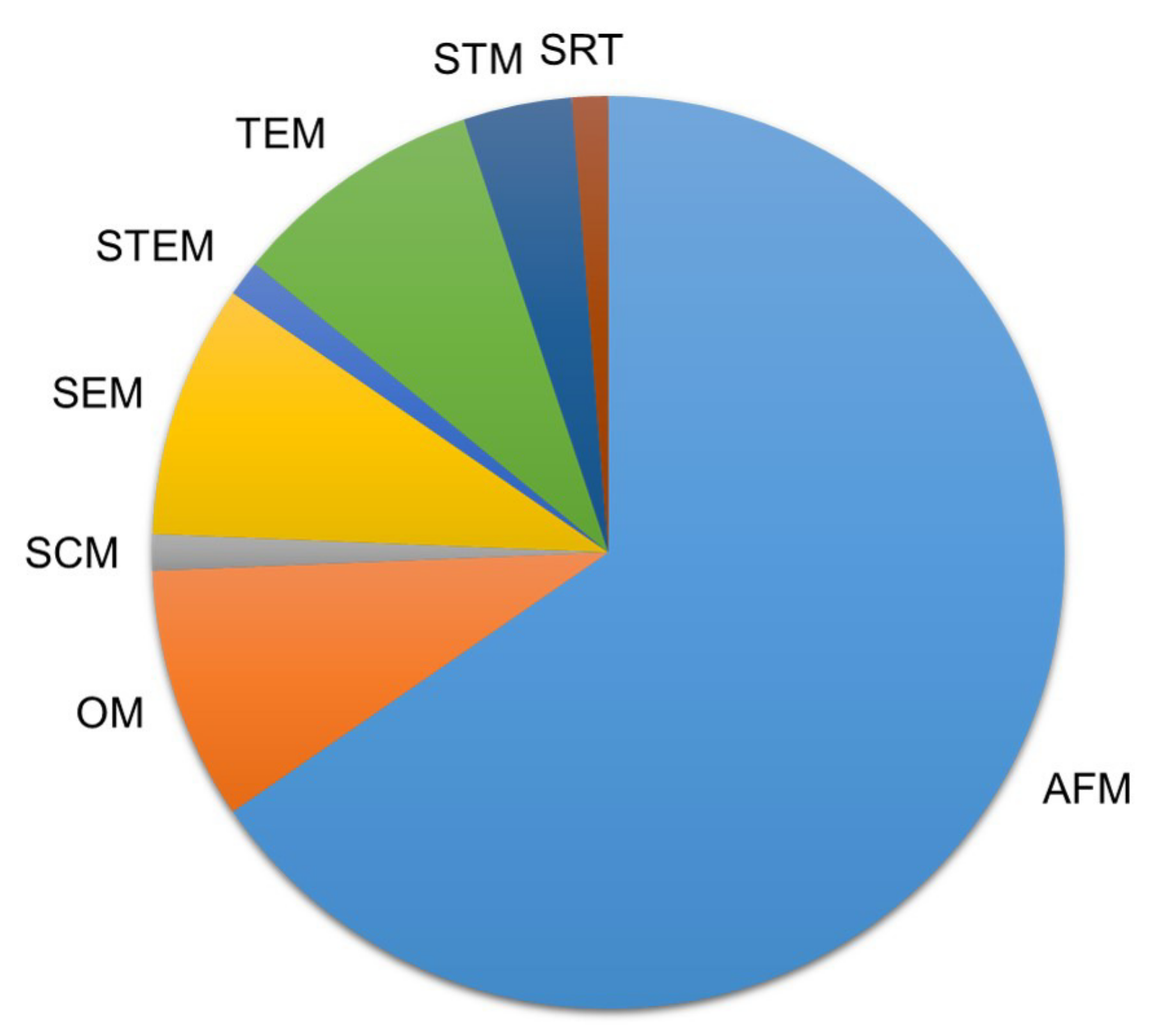
For fractal analysis of thin films, the calculation results of the FD affects by the characterization of film surface, i.e., acquisition of surface data. The usage ratio of characterization methods for fractal calculation of thin film is shown in Figure 1 based on the data statistics of the literature, which can be referred in detail in Appendix A. It can be noticed that atomic force microscopy (AFM) is used most commonly to measure the surface topography of thin films. AFM is based on the closed-loop feedback of weak interaction force signals to obtain the surface topography, so it outputs image height data directly. Except the topographic images with height matrices obtained by AFM or scanning tunneling microscope (STM), the grayscale images obtained by using other instruments such as scanning electron microscope (SEM) have been reported to carry out fractal analysis. However, the FD value of such grayscale images can be different from those of AFM or STM, because the grayscale is not directly relevant to the height of a measured position. In some studies, the grayscale images output by SEM needs to be transformed into topographic data, and then used for subsequent calculations [32,33]. The directly acquired topography data of AFM is more suitable for fractal analysis than the converted data [34]. The calculation results of FD between the two methods are quite different. Therefore, it was necessary to pay attention to the source of topographical data before fractal analysis.
2.3. Calculation Methods for FD
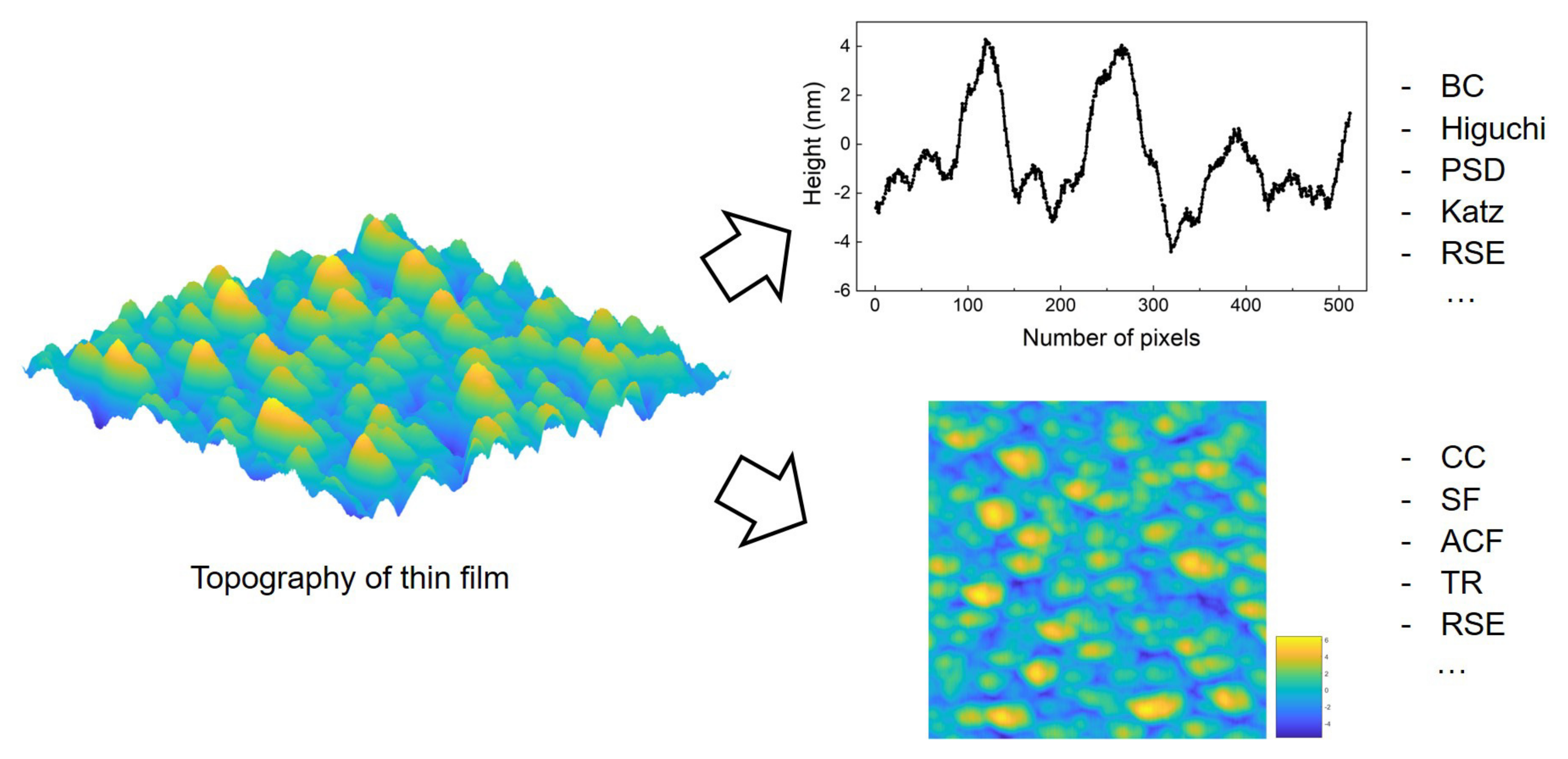
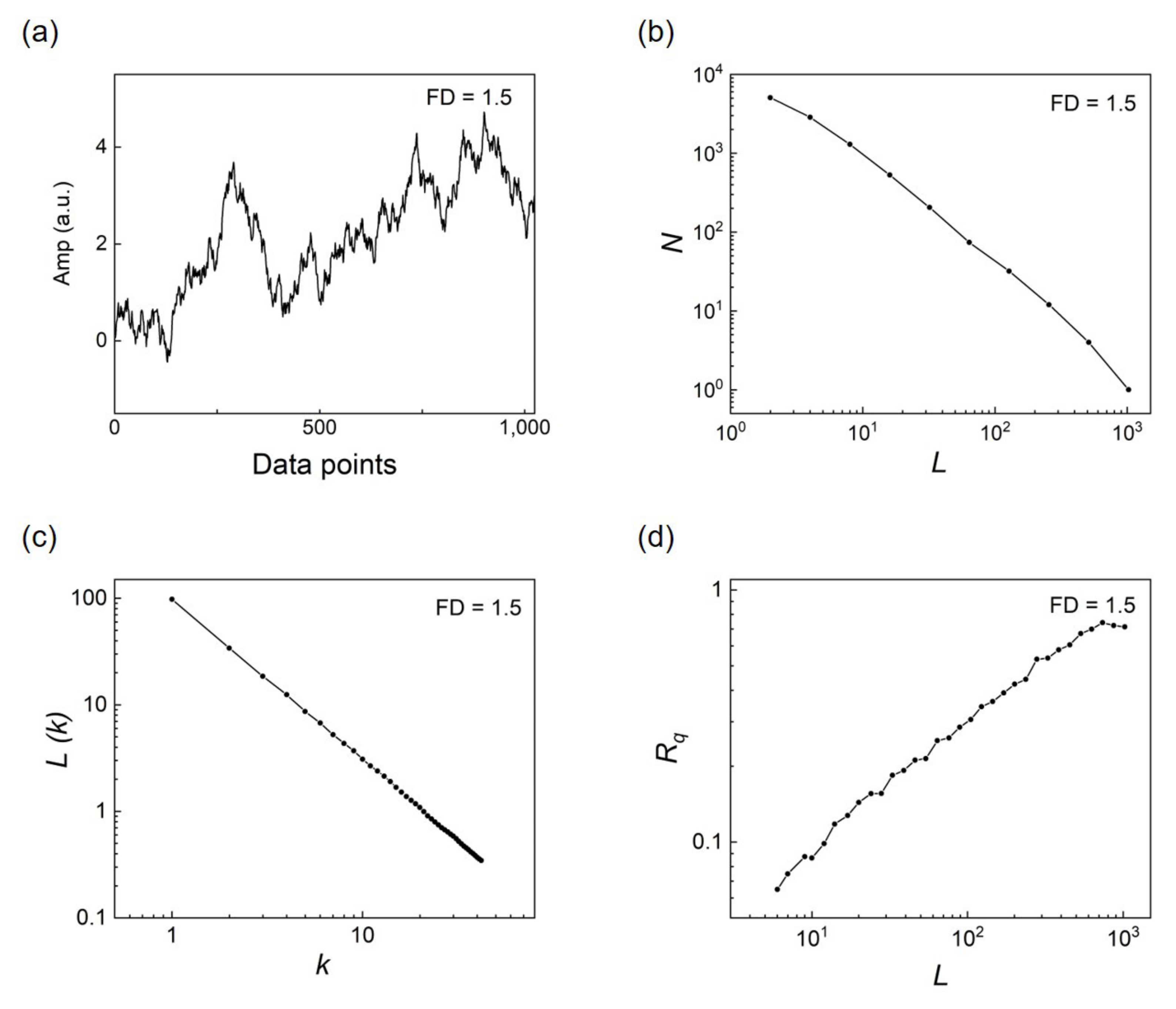
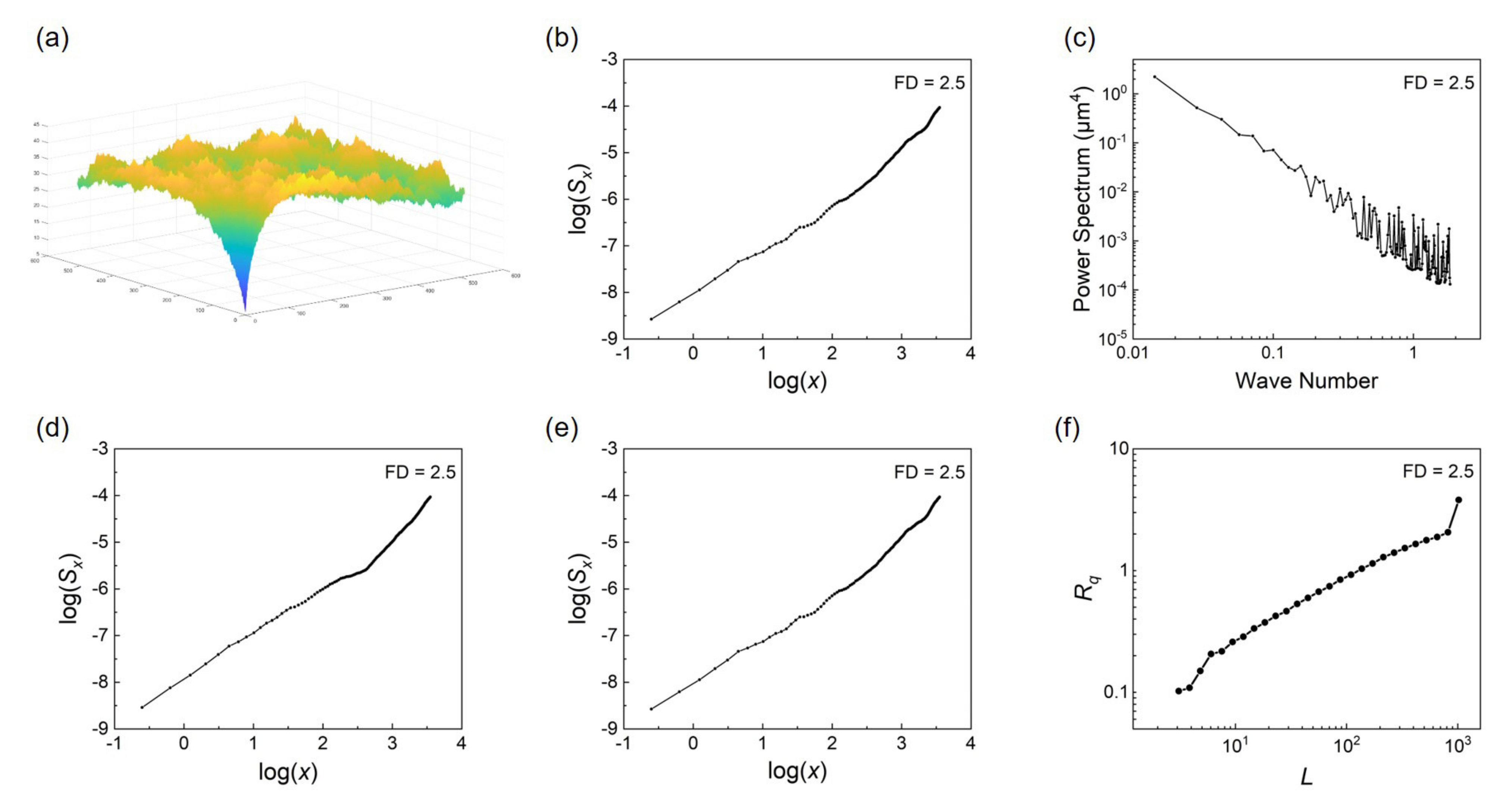
With the wide application of fractal geometry, a variety of FD calculation methods have appeared, such as the BC, SF, ACF, PSD, TR method. According to different calculation principles, the above calculation methods can be roughly divided into scanline-based methods and image-based methods. The former are based on the profile, which referred to a standard height profile as . The latter are based on topographical images directly, which refer to a point plot of height matrix as . The data forms of profile and topographical image are presented in Figure 2. The procedures of calculating the ideal fractal profiles and surfaces with different methods are shown in Figure 3 and Figure 4, respectively. The specific calculation equations and solutions of these methods are demonstrated in Section 2.3.
2.3.1. Scanline-Based Methods
- (1)
- Box counting method
Liebovitch et al. [35] proposed the BC method, to calculate the FD of dynamic and iterated function systems. The profile point set is completely covered by boxes of size , and is the minimal number of boxes. Hence, its FD () can be expressed as follows.
In order to calculate FD easily and clearly, it could be written as follows,
where C is a constant value. In the double logarithmic coordinate system, could be obtained by fitting the slope of the straight line with the least square method, as Figure 3b.
- (2)
- Higuchi method
The Higuchi method is a fractal method for time/space signals. For surface data, the FD is calculated by extracting profiles from surface topography. The specific calculation process [36] is:
Step 1: Set a time series of length N, and use the delay method to reconstruct the time series into the matrix as:
Step 2: Each curve length is defined as:
Step 3: The total sequence length is similar to the average of the lengths of the k delay-generated sequence curves,
Step 4: Obtain the curves for different k and . If it is a straight line, it means that exists. FD can be obtained by fitting in double logarithmic coordinates as Figure 3c. The Higuchi method has higher accuracy in calculating the FD of time series, but the setting of in the realization process is relatively vague. In realistic application, empirical or hypothetical values are often used, which lead to uncertain risks to the accuracy.
- (3)
- Power spectral density method
Surface topography can be considered as a series of signals in the spatial domain, and the power spectral density can describe the topography from a frequency perspective. Changing the measurement scale L of the surface topography is equal to changing the cutoff frequency at the view of the signal. If a surface topography is fractal, then the shape of the spectrum remains the same, even if the observation scale is changed. Thus, the fractal curve is as follows:
where , and is FD of the profile.
The power spectral density method can quantitatively describe the frequency spectrum, and provide abundant information [37]. However, it can be seen in the previous description that the calculation process is based on a linear topography rather than a surface topography. In order to calculate the FD of a whole surface, in the PSD method, it was common to disassemble the surface into a series of profiles, and calculate all their FD values. By adding 1 to the average FD of profiles, FD can be obtained. This calculation process greatly reduces the reliability of the results.
- (4)
- Katz Method
The Katz method was proposed by Katz [38] in 1988 to evaluate the FD of electroencephalography (EEG). It can be regarded as a collection of a series of points , where represents the gradual increase of time. The following is the calculation formula of FD (D) in the Katz method.
where n is the number of intervals between the midpoint of the waveform point column, i.e., , and represents the maximum plane diameter range of the waveform (i.e., the maximum distance from the starting point of the waveform to any other point), and L refers to the Euclidean geometric length of the waveform. The Katz method is considered to be an algorithm reflecting time-domain amplitude characteristics of signals, which has relevant applications in the fault diagnosis of bearings and gears.
2.3.2. Single-Image-Based Methods
- (1)
- The Cube counting method
The essence of cube counting (CC) and the BC method is the same. BC is used for two-dimensional profile and CC is used for surfaces. Some reports also refer to CC method collectively as BC. For the fractal surface topography, a cube (or sphere) with side length is used to cover it, and the minimum number of cubes required is . Changing the side length of the cube obtains a series of . When , there is the relationship: , where is the FD. Therefore, the equation of this method is as follows:
Limited by the resolution of the measuring instrument, the interval between the data points of the surface topography obtained by actual measurement cannot be infinitely small, resulting in a surface topography with limited resolution, and the ratio between the height and width of the surface topography is large. Therefore, in practice, a cuboid with a scale of is usually used to cover the known surface topography. The value of is usually selected from 100 to 1000 (according to the ratio of the height or the pixel width). The minimum number of cuboids required is . The FD is calculated by the slope K of the line fitted in a double logarithmic coordinate, as Figure 4b. The relationship between and the slope K is .
The BC/CC method is one of the most classic FD calculation methods and widely used in various fields. This method can obtain FD from a single image, but the disadvantage is that the calculation accuracy is relatively low.
- (2)
- Structure function method
In surface topography, the structural function of a spatial sequence with fractal features is Equation (15).
where represents the averaging operation. The slope K of is fitted by a straight line in a double logarithmic coordinate, as Figure 4d, and its FD is , where . For the surface topography, the FD of each profile must be calculated and the average value is calculated, and the value of the FD of the surface topography is . The structure function method is suitable for self-affine profiles of engineering surfaces and can provide good results. However, as its FD must be transformed from the profiles to a surface, the accuracy is still not very high.
- (3)
- Autocorrelation function method
For a spatial sequence in the surface topography, its autocorrelation function of the spatial sequence with fractal characteristics is:
The structure function has the following relationship with the autocorrelation function:
Therefore, the ACF method can be converted into a structural function method for calculation.
- (4)
- Height-height correlation function
Vicsek et al. linked the spatial scaling behavior with time, and the concept of dynamic scaling appeared in 1985 [39,40]. During film growth, the interface width w as Equation (18), and the deposition time t exhibit power-law behavior. And obviously t is proportional to the film thickness l. Therefore, the power law can be written as Equation (19), and is the growth exponent. The height matrix of AFM can be analyzed by height-height correlation function, i.e., . Since the actual film surface is continuous, the height obtained by AFM is related rather than independent. Along the scan direction, the height correlation can be obtained in Equation (20).
where m is number of pixel points used in calculation, d is the distance between two pixel points. FD is obtained by fitting a power law of the linear region of the double logarithm curve of and r [41]. As shown in Equation (21), the r value in a certain range can reflect the surface topography, such as self-affine and mounded thin film surfaces [42]. For smaller r, the relationship between and r is exponential, and , where is roughness index between 0 and 1. For mounded surface, r is larger and exhibits oscillatory behavior. Thus, the value of r, when H increase to , is defined as the lateral correlation length . The variation of the lateral correlation with thickness obeys the power law as Equation (22), where z is the dynamic exponent. If the lateral distance between two points is more than , the correlation of them is little.
2.3.3. Multi-Image-Based Method
Roughness is one of the most common parameters that characterize surface topography, but the roughness value is highly affected by measuring instruments, measurement scales, etc. Previous studies have reviewed that there is a strong correlation between roughness and measurement scale, which is associated with the scaling characteristics of surface roughness. Soumya et al. [43] studied the power function relationship between roughness, measurement scale and FD in a fractal surface, as shown in Equation (23).
is the root-mean-squared value of the height measured over the surface; L is the measurement scale, i.e., side length of the scanned area; H is the Hurst exponent. Thus, the FD can be calculated from the slope of a least-square regression fitting line in a log-log coordinate plot of -L.
When comparing the BC/ACF/SF/PSD/TR methods, Kulesza et al. [44] found that the first four can calculate the FD from a single image, but the accuracy of the calculation result is low. Traditional roughness (TR) method has a higher accuracy, however, it requires a series of images with different measurement scales, leading to a decrease in calculation efficiency. To deal with this shortcoming, roughness scaling extraction (RSE) was proposed [24] based on the scaling effect and the robust of roughness against low image elements [45].
2.3.4. Roughness Scaling Extraction Method
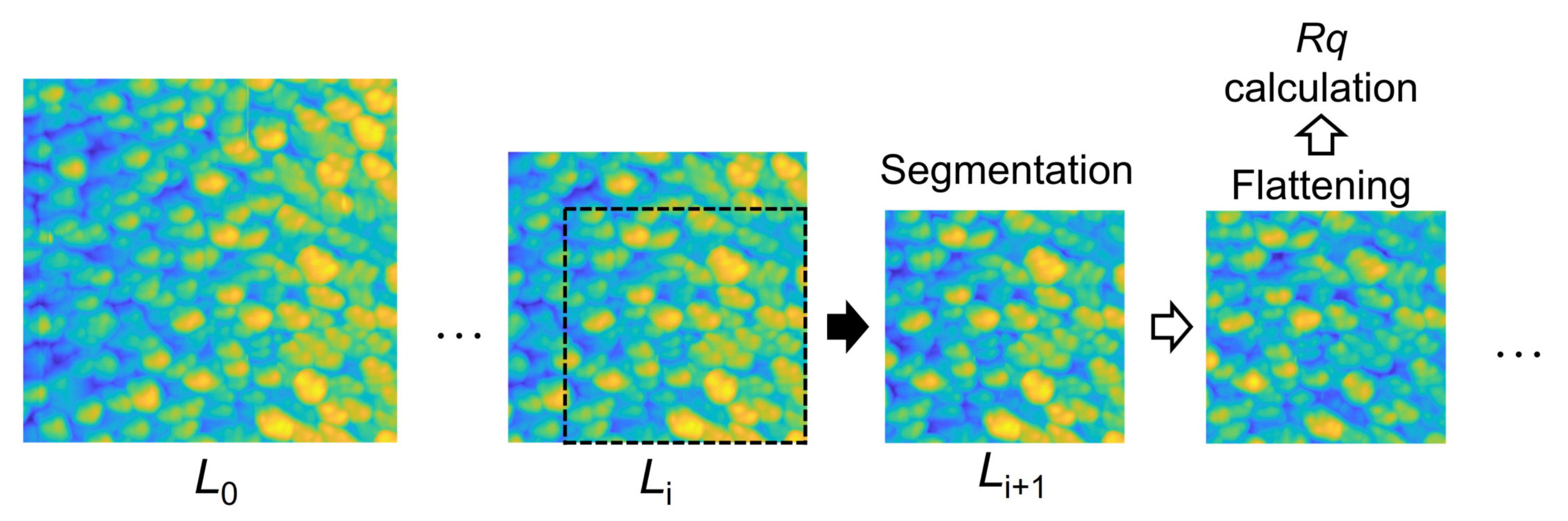
The RSE method was found to be effective to analyze thin film surfaces [24], the morphological filtering effect of AFM measurement [27] and time-series signals such as EEG [23]. Similar to the TR method, the RSE method is also based on the scaling characteristics of surface roughness shown in Equation (23) and Figure 5; otherwise, the robustness of roughness at low image-resolution is another vital theoretical basis that ensures the validity of the segmentation process. Therefore, the RSE method only requires a single topographical image of the concerned surface. The sub-images at different scales are obtained through segmentation of the original image. Due to the inclination and waviness of the sample surface, the roughness value calculated directly based on the sub-images is significantly higher [5], so the flatten modification would to be carried out for all the sub-images to obtain a more accurate relationship between and L.
The flatten modification procedure firstly involves fitting the sub-image matrix and then subtracting the fitting matrix from the original one, in order to remove deviations of the sample surface due to large-scale bending, tilting, etc., so that the high-frequency details of the topography surface is enhanced. The overall procedure of RSE is shown in Figure 6. There are two methods of flattening modification: scanline flattening (RSE-f) for per-row/column data and surface planarization (RSE-p) for image matrix data. The order of flattening modification includes 0, 1, 2, etc., depending on the order of the utilized fitting function. RSE-f1 is used in the following because of its balanced performance of both high efficiency and accuracy with a mean relative error of about 0.64% [24]. The RSE method can not only accurately calculate the FD of a surface, but also acquire a reliabe -L curve during the process, which can quickly obtain the roughness of the surface at other scales.
3. Mechanism and Techniques of Thin Films
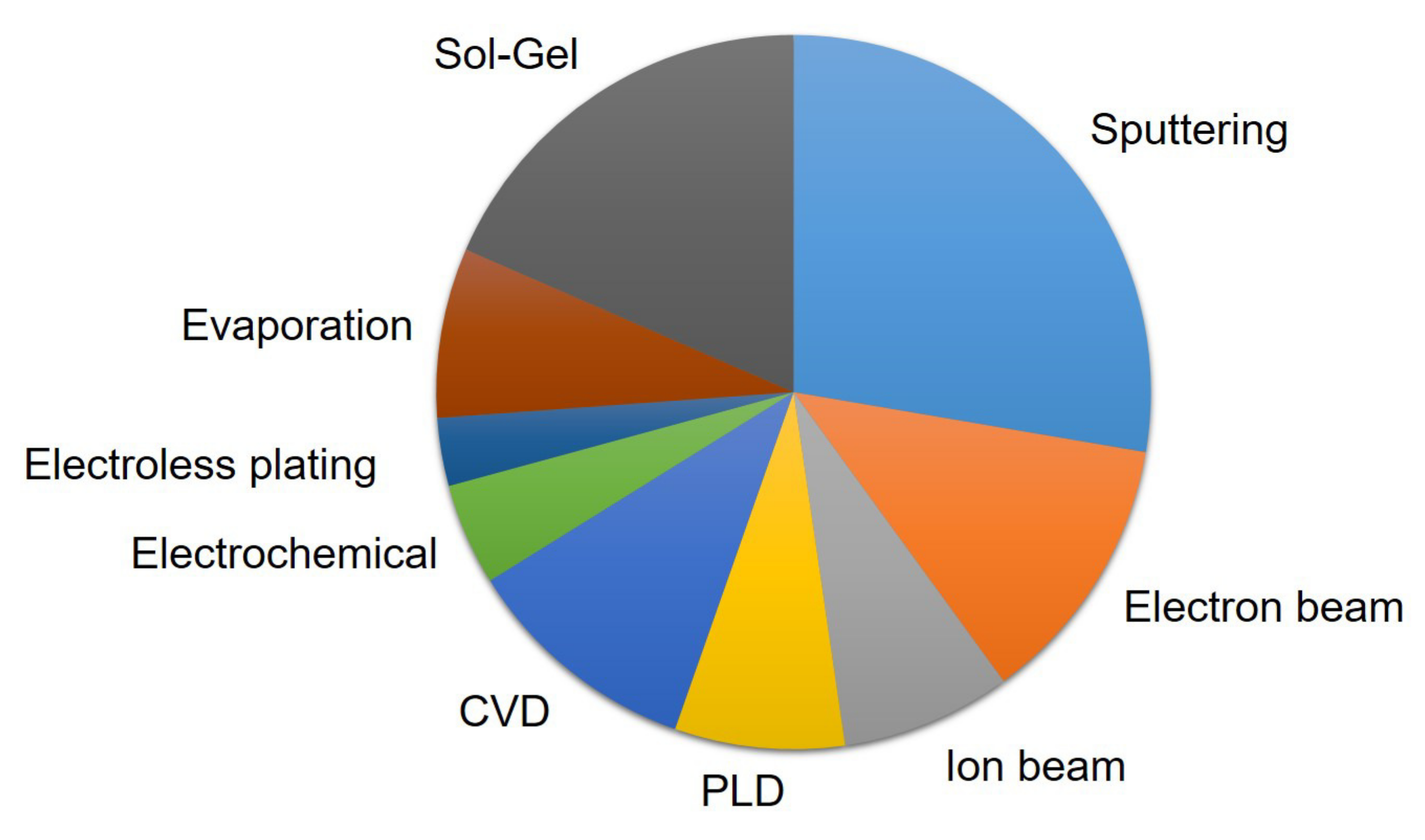
Many thin film surfaces, machined surfaces [2,46,47,48], and other treated surfaces have been shown to have fractal properties. In the field of surface engineering, the surfaces have different degrees of fractal topography, which leads to different performance of the functional film [37,49]. In the field of thin films, different substrate surfaces and preparation methods lead to different fractal micro-structures. In the field of tribology, the fractal characteristics of surfaces affect the state of friction and wear [50,51]. Many theoretical and experimental studies have shown fractal features in various thin film structures. The ratios of the preparation methods in the literature are shown in Figure 7. In previous publications, the applications of fractal analysis obtained more valuable findings than traditional roughness characterization, which was helpful to study more comprehensive surface quality assessments and the study of topography formation and film growth mechanisms. The applications of fractal analysis in various thin films using different preparation methods are introduced in this sections. The films investigated in this review were prepared with physical vapor deposition (PVD), chemical vapor deposition (CVD) and non-vacuum methods, and their surfaces were analysis with fractal methods.
3.1. Surface Growth and Factors
In surface growth, clustering and diffusion of atomic or molecule affect surface topography of thin films at the micro scale. Roughness index and dynamics index can be calculated by surface growth model. The surface growth model is expressed by nonlinear partial differential equation, and partial differential of time-variable is expressed by space-variable partial differential derivative. Edwards-Wilkinson equation [52], Kardar-Paris-Zhang equation [53], Lai-Das Sarma equation [54], and Kuramato-Sivashinsky equation [55] can express the process of particle deposition and accumulation into film under chaotic dynamics. However, the order and variable of the expression are different, so the numerical solution of nonlinear partial differential equations in dimension needs further discussion.
For Edward-Wilkinson equation, it can be expressed as Equation (24), where is Gauss white noise.
For Kardar-Paris-Zhang equation, it can be expressed as Equation (25).
For Lai-Das Sarma equation, it can be expressed as Equation (26).
For Kuramato-Sivashinsky equation, it can be expressed as Equation (27).
The two common statistical models of sedimentary processes are random deposition and ballistic deposition. In the two deposition methods, fractal model can simulate surface height of thin films and reveal growth mechanism to some extent. Ghosh et al. found that the roughness index of the ballistic deposition model calculated by FD fitted with the calculated value of the Kardar-Paris-Zhang continuum growth model [56]. Qi et al. verified the fractal characteristics in the film growth process in Kuramato-Sivashinsky model [57].
The deposition process and final morphology of films are also influenced by shadowing and diffusion effect. The cause for shadowing is that the higher part of the angular surface topography blocks the lower part, resulting in different particle fluxes received at different locations on the surfaces. The film grows in columns, eventually forming mound on surface [58]. In oblique incidence flux and substrate motion, different deposition angles can affect deposition effect of shadowing [59]. When the fractal surface is affected by different degrees of shadowing, FD is also affected. In the shadowing effect model, the shadowing function is a function of incident angle , RMS slope and observation length L. The RMS slope is a function of FD, so the shadowing function is related to and FD. The rough surface with larger FD has a more significant masking effect [60,61].
To quantify a fractal surface, except FD, there are some advanced fractal parameters can be used as surface entropy, fractal succolarity and fractal lacunarity. Surface entropy is used to describe the height distribution homogeneity [62], which influences the chemical structure and surface tension of surface at micro or nanoscale [63]. The value of surface entropy varies between 0 and 1, with 0 representing maximum heterogeneity. Being close to 0 of surface entropy may indicate topographic irregularities and problems in adhesion [64]. Fractal succolarity relates the intercommunication in a surface [62], which can be seen as the degree of surface percolation. For the film surface, it is assumed that there is fluid entering the upper band of the surface, and the channels composed of similar points can assist fluid to the lower band. Penetration into the inner layer through such a process is the phenomenon of percolation [65,66]. Fractal lacunarity quantifies the distribution of gaps in space as a function of scale [67]. A lower fractal lacunarity indicates that the gaps are uniform, and the surface can be indirectly considered to be homogeneous [63].
3.2. Physical Vapor Deposition
3.2.1. Electron Beam Evaporation
Electron beam evaporation (EBE) heats and vaporizes coating material by accelerated electrons. The kinetic energy of the electrons is mostly converted into thermal energy, thereby achieving evaporation. This method has a high evaporation rate and a high purity of the film, and is suitable for fabricating thin films with a high melting point.
Pandey et al. [68] studied BaF2 thin films prepared on three different substrates of Al, Si, and glass, and they calculated the average roughness, interface width, and surface FD. It was found that the FD values of the film on a glass substrate in the horizontal and vertical directions were close, indicating isotropy. The FD of the BaF2 film on the Si substrate was higher than the others, indicating that the surface topography was highly complex. The variation of Hurst exponent and crystalline size with thickness on different substrates was systematic studied, which contributed to growth mechanism understanding. Yadav et al. [20] also studied BaF2 thin films, and analyzed topographical changes over the growth of thin films through roughness , interface width, and FD. Among them, the FD and multifractal approach were mainly used as complexity measures to demonstrate the geometrical and physical characters of ions irradiated surface, which were excellent tools for characterizing surfaces.
The general finding in those reports is that fractal structure actually exists in the EBE films. FD can exclude the influence of the scale effect, which is different from roughness. Hence, using fractal analysis is more direct to study the relationship between the surface topography and substrate material, preparation parameters, etc.
3.2.2. Pulsed Laser Deposition
Pulsed laser deposition (PLD) irradiates target with a focused laser pulse, generating a strong laser spray plume. Evaporated atoms in the melt beam are then deposited on the substrate and form a thin film. Through the PLD method, the crystalline state (size distribution and shape of nanocrystals) and the adhesion to the substrate can be controlled by changing the target-to-substrate distance, background pressure, substrate temperature, laser flux and other parameters. As reported, too many parameters could affect the PLD surfaces, which could be effectively quantified and compared by fractal analysis.
Soumya et al. [43] studied ZnS thin films prepared with the PLD method at different annealing temperatures and analyzed the surface topography based on AFM image data. A strong correlation was found between the annealing temperature, surface roughness and FD. Singh et al. [69] studied multiferroic BiFeO3 films prepared on Si, STO, and sapphire substrates, and they calculated the FD of the topography profiles in rows and columns respectively. It was found that all the samples shown the anti-persistence behaviour by fractal analysis of Hurst exponent, and the anisotropic level on different substrates can be suggested by FD value.
3.2.3. Magnetron Sputtering Deposition
As one of the PVD methods, magnetron sputtering deposition is commonly utilized in the preparation of thin films. The theory is to bombard the target with hundreds of eV ions accelerated in an electric magnetic field. Target atoms obtain energy, and are sputtered into the gas phase. The sputtered atoms re-agglomerate on the substrate and then form a thin film. In the meantime, the secondary electrons generated during sputtering are bound by the electric-magnetic field in the plasma region on the target surface, so a large amount of ions are continuously ionized to bombard the target to improve the deposition rate. In 1999, high power pulsed/impluse magnetron sputtering technology was proposed by Kouznetsov et al. [70], which combined the advantages of high intensity arc technology and magnetron sputtering, attracting attention for its high metal ionization rate. High power impluse magnetron sputtering can improve film quality, reduce surface roughness [71], intensify adhesion of film and increase hardness and strength [72].
Wang et al. [37] applied the fractal theory to analyze the surface topography of a Cu-W thin film during the growth process, and explored the relationship between FD and the resistivity of the thin film. It was found that the surface roughness of the thin film was caused by high-frequency components. As the deposition time increased, the thickness and FD of the film increased. In addition, for the film surface of the uniform phases, the resistivity was positively correlated with FD. Similarly, Talu et al. [73] analyzed the surface topography of Ag-Cu thin films at different deposition times and found that as the deposition time increased from 4 to 24 min, the particle size and FD both increased and then decreased. The resistivity was then found to be negatively correlated with deposition time, which was ascribed to the increment of the contacts between particles. In these reports, FD can be used not only to evaluate surface complexity, but also to study its correlation with film properties.
The thin film growth is affected by the fabrication parameters and is shown in the analysis of FD. Talu et al. [74] studied the effect of annealing temperatures on the surface topography of C-Ni thin films, and analyzed the correlation between the surface texture characteristics and the length scale. Meanwhile, there were two corner frequencies in the profile for calculating the FD, and their values were positively correlated with tip radius and cluster size respectively. Fang et al. [75] analyzed the nano-friction and wear characteristics of ZnO thin films deposited at different sputtering powers. Moreover, the higher sputtering power led to smoother surfaces, lower FDs, a more pronounced preferential orientation, and larger nano-wear rate.
Feng et al. [76] used the RSE method to perform fractal analysis on MgO thin films prepared by the energetic partical self-assisted deposition (EPSAD) method. The FD values of MgO films under different preparation were compared to reveal deposition mechanism during the EPSAD method. Talu et al. [77] focused on zinc oxide film, calculated multiple fractal characteristics of the 3-D texture on the surface based on AFM measurement, and proved that there was a significant correlation between the fractal features and the surface texture. Talu et al. [32] also studied the surface texture of Cu/Co thin films and established a set of friction mathematical models including , kurtosis, FD, and corner frequency, from nanoscale to macroscale, so that the friction properties of the films could be controlled and modified. To understand material science such as crystal growth, defects and phase transformations, fractal analysis contribute to explaining the relationship between topography and material performance.
Based on the above reports, FD as the complexity of the film surface is affected by the film preparation parameters. On the other hand, it can be related to the application performance. As an intermediate parameter, the selection of preparation parameter could be optimized according to the FD trend to obtain the desired application performance.
3.3. Chemical Vapor Deposition
CVD refers to the method of depositing thin films by a surface chemical reaction with the raw reaction materials being gaseous and at least one of the products being solid. Compared with PVD, CVD applies a vapor phase reaction, by which the surface can form films with a high production efficiency and performance consistency. The preparation process and parameters of CVD and PVD are different in principle, but the fractal properties of thin films fabricated with both methods have been reported.
Talu et al. [78] studied the three-dimensional surface texture of amorphous hydrogenated carbon by the different power of radio frequency-plasma enhanced CVD, and the analyzed parameters includes FD, pseudo-topothesy, anisotropy ratio, skewness, kurtosis, and roughness. Those function allowed for a reasonable prediction of space patterns. The statistical, fractal, and functional surface properties of films contribute to a characterization of micrometer- and nanometer-scale textures. Haniam et al. [79] synthesized a fractal thin film of cobalt oxides by using CVD, and its density and crystallization were affected by various factors, such as laser irradiation time and the gas flow ratio. This meant that the fractal structures could be controlled in CVD process. Fractal structures described by diffusion-limited aggregation model and compared with the FD of the growth pattern by box counting. Li et al. [80] built a 2D diffusion-limited aggregation model, which was based on a typical model of fractal theory. By this model, the CVD growth of various fractal-morphology 2D materials were precisely controlled. Fractal-growth theory applied to CVD-growth process provided favourable predictions for fabrication parameters.
3.4. Non-Vacuum Methods
3.4.1. Electroplating Method
Electroplating is the process of plating a thin layer of metals or alloys on the surface of a substrate using electrolysis, which can enhance the corrosion resistance of the metal, increase hardness, and prevent wear.
Nasehnejad et al. [81] calculated the surface FD of Ag films with different thicknesses. The film thickness increased from 250 to 750 nm, and the FD increased from 2.57 to 2.64, indicating that, during the deposition process, as the deposition time increased, the irregular shape of the surface became more prominent. Naseri et al. [82] analyzed TiO2 thin films prepared at different current densities and found that extremely low or high current densities cause anisotropic structures of the films, but medium current densities would cause uniformly decorated tubes, and the FD was also lower. Gholamreza et al. [83] studied Ag films obtained from different deposition current densities and substrate rotation speeds. The higher the rotation speed, the larger the FD value was, and the FD could be used to describe the change in the overall topography along the growth direction. Fractal analysis provides the lateral development of surface features [42], and it is useful for understanding the growth and scaling of thin films during formation.
3.4.2. Sol–Gel Method
Sol–Gel method is a process of converting sol, a colloidal suspension of solid particles in liquid [84], into thin films by coating and heat treatment [85]. The unique features of the sol–gel process, including the chemical reactions, the ease of doping, and the low synthesis temperature, were conducive to the preparation of industrial coatings.
Ghosh et al. [86] studied the surface microstructures of sol–gel spin coated ZnO thin films in varying precursor quantified by Higuchi method. There was a certain correlation between grain size and the Hurst exponent, and larger average grain sizes were attributed to higher Hurst exponent values. Pandey et al. [87] analyzed three parameters of Al–doped ZnO thin films by AFM images, were thickness, refractive index and FD. The root mean square interface and FD used to quantify the surface topography decreased with increasing thickness. It was found that increasing film thickness, corresponding to densification and a growing number of hillocks, may contribute to the refractive index.
3.5. Parameters Related to FD
In traditional surface analysis, roughness is often used to evaluate surface quality at the micro-scale. However, due to the scaling characteristics of surface roughness, it is difficult to compare the roughness at different scales. A surface with many fine structures and a high degree of fragmentation might have a lower surface roughness value, but the actual corresponding quality does not meet the engineering requirements. Therefore, it is difficult to characterize the essential characteristics of micro-engineered surfaces based only on roughness. Previous studies have found that fractal phenomena exist during the nucleation and growth processes of thin films at the microscopic scale. Thus, fractal theory contributes to a comprehensive characterization on surface topography.
As a scale-independent parameter reflecting the surface microstructure properties and surface quality, FD has a strong correlation with preparation process parameters and topographical parameters.
In terms of the preparation process, common process parameters include deposition time, sputtering power, and annealing temperature. Trends reported in some articles were summarized, but corresponding to specific preparation methods and topography, researchers still have to use FD to explore the rules. As the deposition time increases, the irregular shape of the surface becomes more prominent, and the value of FD increases accordingly [37,63]. As the sputtering power increases, the preferential orientation of the grains becomes more pronounced [75,76], and the FD decreases. As the annealing temperature increases, the atomic mobility increases and the FD decreases [27,43,88].
In terms of topographical parameters, the change in FD is consistent with cluster size formation, which is usually interpreted as follows. The formation or aggregation of island-like structures on the surface is often manifested by an increase in cluster size, which causes the rise of surface complexity, and thus the value of FD increases. Moreover, in the process of calculating the FD, the corner of the -L curve is usually related to the tip radius and the size of the clusters. In addition, the FD of the profiles in different directions of the topography can be used to quantify the anisotropy of the film.
At present, the relationship between fractal parameters and film surface characteristics and topography cannot be predicted [42]. It is necessary to conduct fractal analysis of specific films and attempt to explore the relationship between FD and performance parameters. Though fractal results, the fabrication parameters can be modified.
4. Factors and Effects of Fractal Properties
4.1. Fractal Study of Various Thin Films
In investigations of thin films prepared by different technologies, previous studies have repeatedly found that the microstructure of the topography appearing in the growth process of the films exhibits fractal properties. The FD can be used to measure the complexity of the topography and explore the effect of preparation conditions on topographical quality [89,90]. In recent years, different methods have been used to calculate the FD of various thin films, and the results are summarized in Appendix A.
For the FD value, firstly, it limited by the definition range. The FD for profiles is between 1 and 2, and it is between 2 and 3 for the topography surface. Secondly, the FD value difference of the same type of film under different preparation conditions is almost within 0.5. The FD value directly reflects the irregularity of the surface topography, and the deposition state during film preparation can be characterized by the Hurst exponent. Hurst exponent is also often used to evaluate the randomness of the time series. The relationship between H and D is shown in the Equation (28).
(1) When , the time series has a long-range correlation [81], i.e., an increasing (decreasing) trend over a certain period of time, and an increasing (decreasing) trend in the next period, and the closer H is to 1, the stronger the correlation is.
(2) When , the time series is irrelevant and is an independent random process; i.e., the current state does not affect the future state. The change at any time step is uncorrelated with the change of previous or later steps.
(3) When , there is only negative correlation in the time series, showing an anti-persistent state [91], i.e., the time series is increasing (decreasing) in a certain time period, and then decreasing (increasing) in the next time period.
The value of H ranging 0.5 to 1 can be found if there is a long-range correlation (also known as long memory) during the preparation process [92], which can provide detailed information on cluster growth and surface formation regarding continuity.
4.2. Application of Fractal Calculating Methods
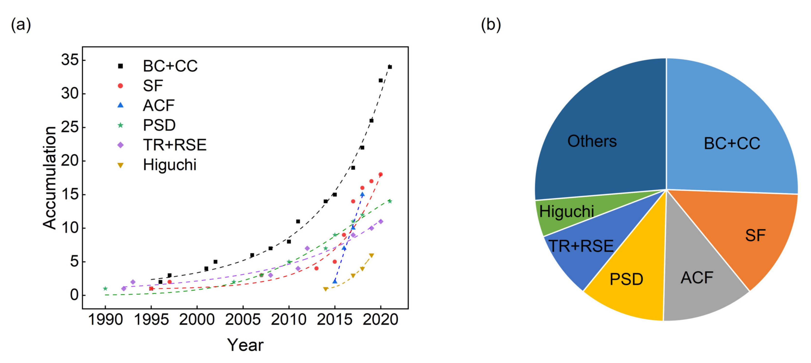
During the development of fractal theory, the calculation method of FD was constantly being updated, and was increasingly used in the topography of thin films. To investigate the utilization of different fractal methods in recent decades, a schematic diagram of the development in accumulative count of studies using a certain FD method over time is shown in Figure 8a. It can be seen that classic fractal calculation methods of BC and CC are the most commonly used in the field of surface topography analysis. Although the Higuchi/SF/PSD methods had been proposed as early as the 80s~90s, these methods are commonly used for fractal calculations of time series, such as signals. In recent decades, these fractal calculation methods have extended to the surface area and have been widely used in growth mechanism analysis and surface quality evaluations of various types of films. The utilization ratio of these fractal methods is shown in Figure 8b. Representative of traditional methods, BC and CC methods are the most widely used, and various new methods were developed and applied after 2010. The community of thin films is now embracing a significant uprising of fractal analysis on surface topography.
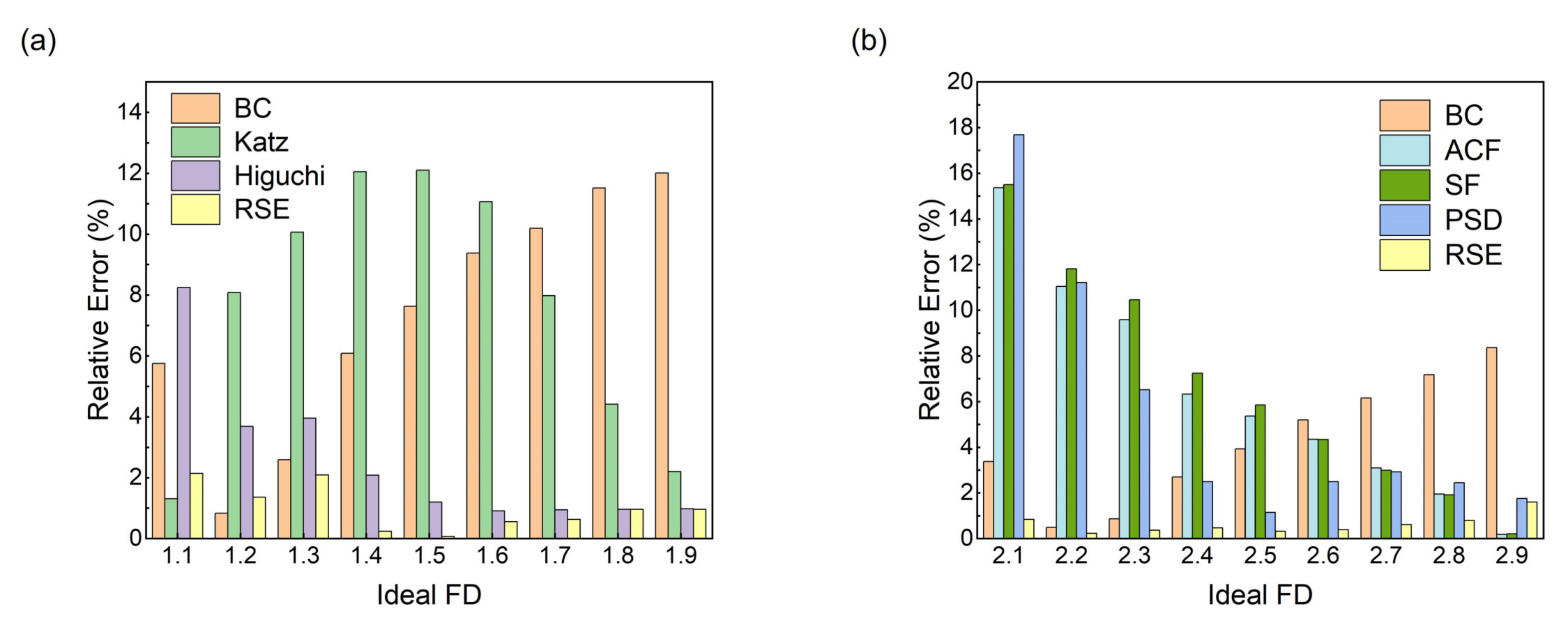
As a core indicator of fractal theory, the FD represents the complexity of fractal geometry. Thus, accurate calculations of FD play an important role in fractal analysis. In order to compare the accuracy of the results of different FD calculation methods, it is necessary to generate surfaces with an ideal FD for verification calculations by mathematical methods. As a general approach, a series of profiles and surfaces with ideal FDs are generated with the W-M function, and FD is calculated using the above methods. In Figure 9, the accuracy of different method is compared. The relative errors of the results calculated with each method significantly different under each ideal FD. For profiles, the calculated results of BC method and KATZ method are significantly different from the ideal FD, even though they are widely used. The results obtained by the Higuchi method are relatively stable when the FD is 1.4∼1.9. For surfaces, in the BC method, when the ideal FD is large, the obtained FD is obviously different from the ideal FD. In the ACF and SF methods, when the ideal FD is low, the calculated FD and the ideal FD are significantly different. In the PSD method, the calculated FD result is relatively accurate only when the ideal FD is larger than 2.4. Therefore, traditional methods cannot provide calculation results of the FD in the full range of the ideal FD (2.0∼3.0) with high accuracy. The RSE method is the most accurate in most cases.
4.3. Reality Issue for Fractal Analysis
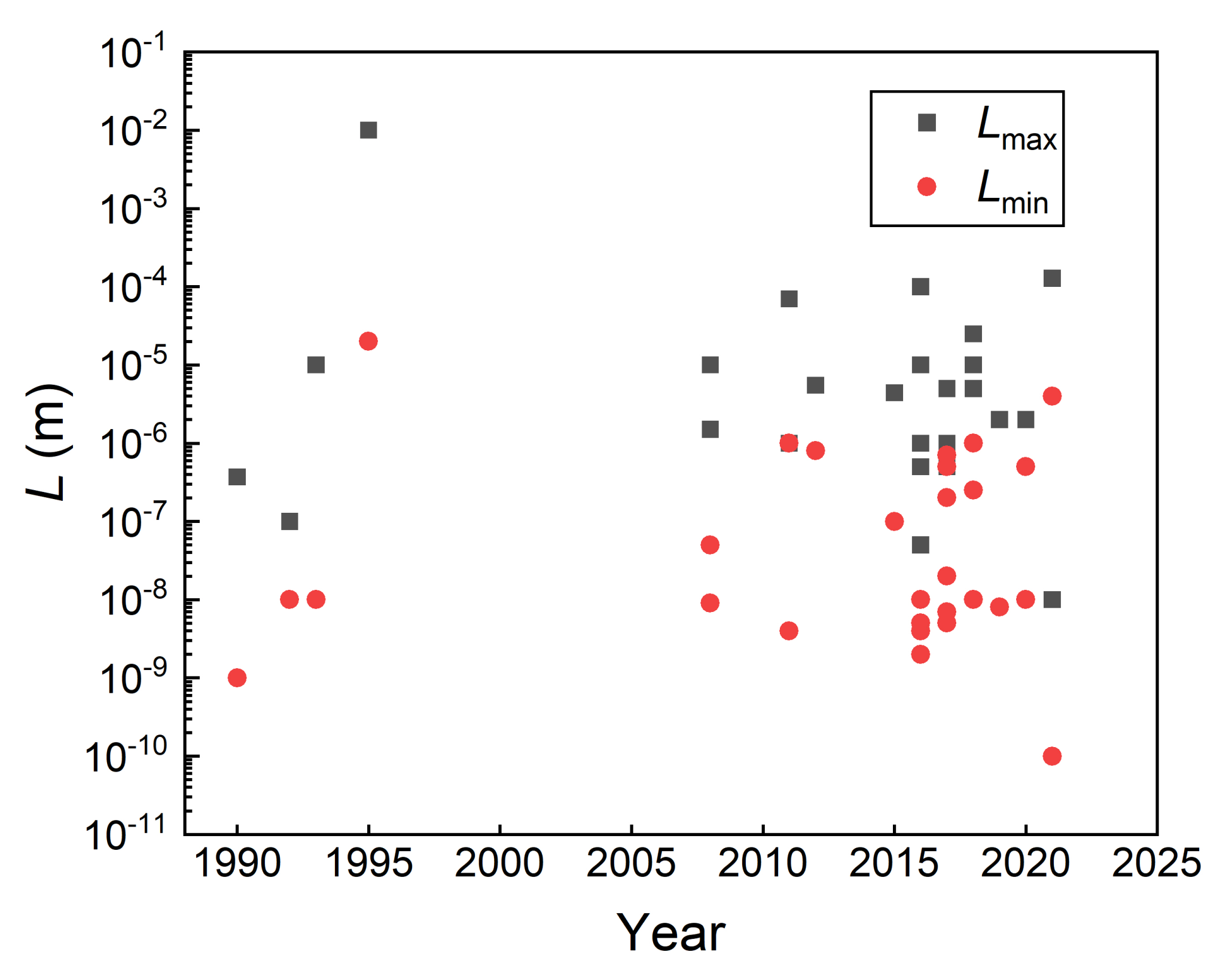
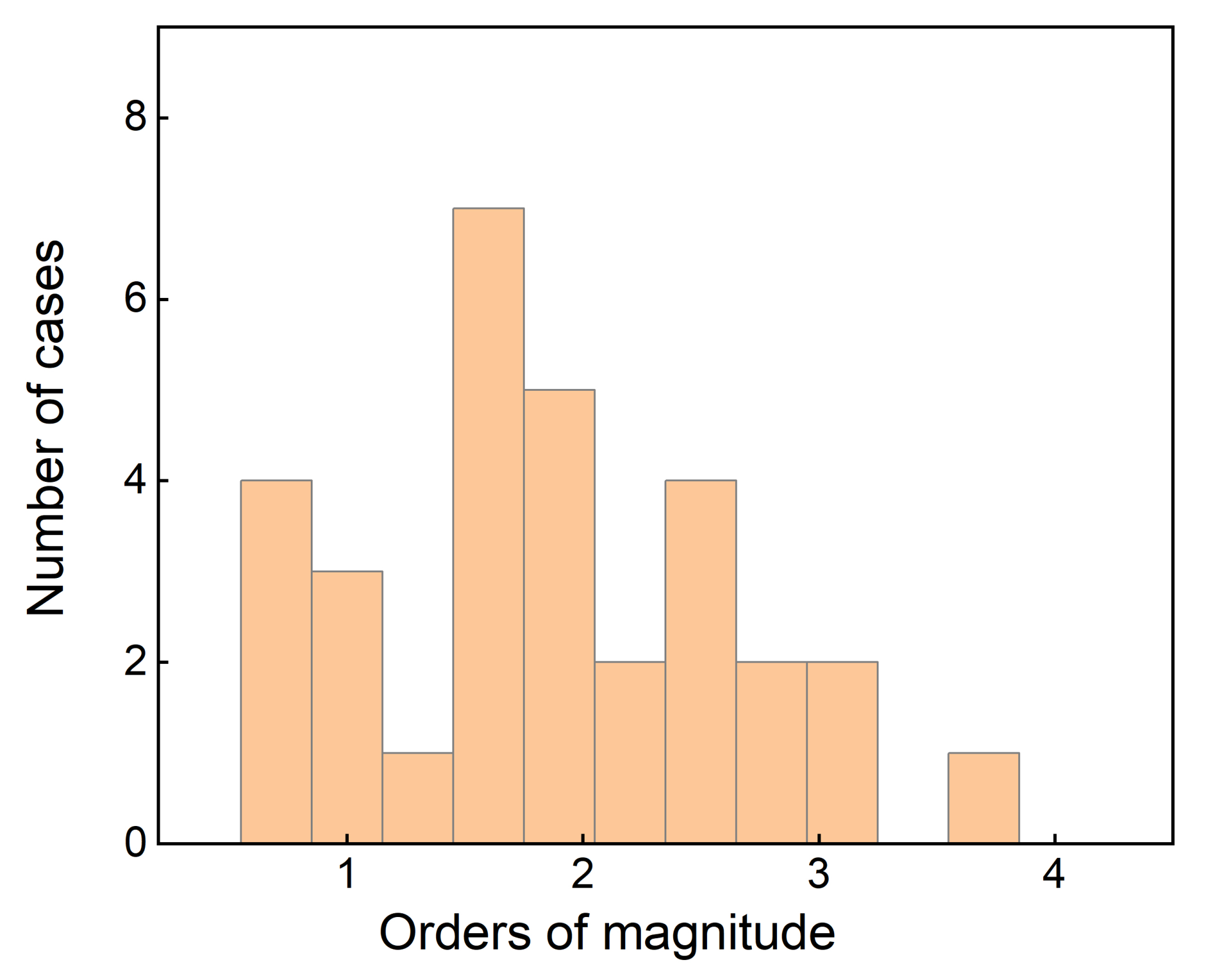
As early as 1998, Avnir [93] noticed that the calculation of FD usually requires the experiment data with a large magnitude span of scales, which centers around 1.3 orders of magnitude in a histogram of this perspective. Based on the extracted data of relevant literature in this study, the maximum and minimum values of scales are summarized in Figure 10. By using the division operation on these values, the magnitude span of scales for fractal analysis of thin films was obtained, as shown in the distribution histogram of Figure 11. The average order of magnitude span in the past two decades in the field of thin films was 1.86. It can be speculated that the enlarging magnitude span relative to the report by Avnir [93] in 1998 indicated an advancement of fractal analysis, which can be attributed to the improvement in surface measurement technology. Currently, the further enlargement of scan scale of AFM is expected, but probe wear could be accelerated due to excessive data collection; thus, a reasonable selection of sampling length could reduce equipment wear, accelerate FD calculations while ensuring the accuracy [94]. There must be further improvements in surface measurements in the next decade.
However, the limitation of a further enlarging of the span might be not technical in the future. The difficulty lying ahead could be the intrinsic characteristics of thin films. As shown in Figure 10, the common maximum scale is around 10,000 nm, while the minimum is around 1 nm. Generally, such a maximum scale corresponds to the typical size of clusters of thin films. If a larger scale is to be investigated, the surface topography is dominated by other factors such as waviness, which are usually dependent on the fabrication process other than cluster growth. The minimum scale is similar to the typical size of stabilized nuclei. If a smaller scale is to be investigated, the individual existence of atoms or ions would be considered, and even the sub-atom structures might be taken into consideration, and these are both quite different from the atomic diffusion process during the nucleation and growth of thin films.
The results and discussion above could be related to the reality issue for fractal analysis, i.e., the scaling region. Fractal analysis can theoretically deal with self-similarity or self-affine features with boundless scales, but the real features in nature are all within a certain range of scales. In 1989, Yokoya et al. [95], when they studied the geographical fractal phenomenon, put forward the argument that fractal feature exists only in the scale range with upper and lower bounds, not a global scope, and the simulation function of fractal Brownian motion was used to derive the specific size of range. The method of cutting the scale-free region based on a genetic algorithm proposed by Fei et al. [96] was applied to the fractal analysis of ground surface. The summation of the average variance can be applied for searching the optimal position of the initial and terminal points. Zuo et al. [97] found that the linearity of the scaling region increased with the sampling length, and the minimum sampling length was greater for a smooth profile than that for a rough profile. The advantage of scaling region interception to improve accuracy was also found in a fractal analysis of EEG signals [98].
For real features in nature, measurement data within the scaling region rather than the global region can invariability exhibit fractal properties with the scale with a high efficiency. When calculating the FD, the linear part in the double logarithmic coordinates can be considered as the scaling region, as shown in Figure 5. Therefore, the identification of the scaling region should play a crucial role in fractal analysis.
5. Prospective Developing Trends
FD is a measure of surface irregularities and discontinuities. Fractal analysis can be associated with cluster size [73,74,75,86], deposition state [37,63,76], topography [69,88], material composition estimations [99] and other parameters to obtain more objective results than the traditional roughness characterization, which is favorable for further interpreting the growth mechanism of thin film surfaces [68,79,83,100]. The specific value and variation trend of FD can play an important role in the comparative investigations of thin films under different conditions. The optimization of calculating FD has also become a principal part of the development of fractal theory.
As the understanding of fractal theory gradually deepens, the calculation of FDs evolves on the basis of traditional methods, and both the calculation efficiency and accuracy are going to be improved. The comparison of mean relative error in this paper assists researchers to utilize the fractal methods with high accuracy.
5.1. Multifractal Analysis for Thin Films
In order to obtain more detailed fractal descriptions, it is necessary to increase the parameters that describe different fractal sets, so the multifractal theory has been developed and applied widely in last decade. A multifractal is a staggered superposition of a large number of single fractals with different dimensions. It is generally characterized by the multifractal spectrum , revealing the complexity and singularity of a class of topography, where a determines the strength of the singularity property, and describes the density of the distribution. As an evolution based on single fractals, the multifractal theory is developing fast [101,102,103,104,105] and becoming a powerful tool for surface analysis. It would be promising to open up new research fields for the application of fractal theory and exciting research achievements. Multifractal detrended fluctuation analysis can determine higher-dimensional fractal and multifractal scaling behavior in time series, which can better filter out the trend components of evolution, retain the fluctuation components, and assist researchers to extract effective information [106,107]. Moreover, with the emerging of more indicators for surface analysis (including FD, multifractal parameters and traditional parameters), it would be convenient to establish a practical scheme of machine learning, such as an artificial neural network model [108], which has demonstrated high accuracy and efficiency in fractal analysis.
5.2. Fractal for Surface Mechanism and Properties
Fractal characters are found in natural topography [8], crystals [109], plants [110], retinal blood vessels [111], etc. For the field of surface engineering, research on the growth mechanism of fractal structures and its impact on the practical applications will be further explored systematically.
In terms of scientific theoretical research, the micro model of the fractal growth mechanism has been established to explain the surface characteristics of thin films [80]. However, whether the theoretical model of fractal growth is consistent with the actual film deposition process has not been systematically studied. The details of film nucleation and cluster growth need to be characterized with more powerful instruments for a comparison with the established models. Such work could further explore the principle of film deposition and reveal the formation mechanism of natural substances from a fractal perspective.
In terms of practical application, many of above-mentioned previous studies have linked fractal characteristics with the application properties of specific film surfaces, such as gas sensing characteristics [49], refractive properties [87], wettability [102], capacitance behavior [112], and resistivity performance [37]. Since the artificial surface of fractal structure can characterize rough surface profile [113], which is random but is also multi-scale and self-similar [25], it is also used in modeling research on the effect of surface topography on performance [114,115]. For studies related to rough surface properties, such as contact process [116], surface liquid film evaporation [117], and post-treatment surface structure [118], fractal analysis can be used to model surfaces. Then the FD as surface evaluation parameter, combined with other physical performance parameters. As a parameter for evaluating the surface complexity, FD is a functional carrier that supports researchers to quantitatively associate surface topography with both fabrication parameters and application performance. In the future, such a functional carrier will be used in more researches on scientific questions and engineering applications.
6. Summary
This article presents an overview of main methods of fractal analysis, ranging from calculation methods for FD to simulation methods of fractal characteristics, and a variety of thin film fabrication techniques. In fractal analysis, the simulation of arificial fractals for evalating the accuarcy of fractal methods, the source of surface data, and the calculation method of FD, are introduced in detail. For calculating FD, methods include scanline-based methods (including BC, Higuchi, PSD, and Katz), single-image-based methods (including CC, SF, ACF and height-height correlation function), and the RSE method based on the TR method. By comparing their usage and accuracies, it provides a reference for researchers to choose appropriate fractal calculation methods. Physical vapor deposition methods, such as electron beam evaporation, pulsed laser deposition, and magnetron sputtering deposition, chemical vapor deposition, and non-vacuum methods, such as electroplating and sol-gel are described. The relationship between film deposition parameters and FD was analyzed, along with the current developments in fractal calculation methods. FD as a topography parameter can feedback the process parameters and application properties in the comprehensive characterization. In nature, the scale range in which the fractal structure exists is not global, so it is a reality issue to determine the scale range selected for fractal calculation in thin films. The scaling region, which would affect the efficiency and accuracy of calculations, was discussed by investigating the literature over the past 2 decades. Compared to the result of 1998, the average order of magnitude span expended to 1.86, which is predicted to be further improved. Through the analysis of literature data on fractal calculations of the film surface, future development trends in this field are proposed including multifractal analysis, surface modeling and practical application. In addition to offering a broad introduction to the common methods of film deposition and fractal analysis, this review can provide an extensive set of references and statistical data that can be used by researchers in the fields of both thin films and fractal analysis.
Author Contributions
Data curation, W.Z. and Y.C.; Funding acquisition, P.F. and F.F.; Investigation, Y.C., Z.L. and F.F.; Project administration, P.F. and F.F.; Visualization, W.Z., Y.C. and H.Z.; Writing—original draft, W.Z. and Y.C.; Writing—review and editing, H.Z. and F.F. All authors have read and agreed to the present version of the manuscript.
Funding
This study was supported by National Natural Science Foundation of China under Grant No. 51875311, Guangdong Basic and Applied Basic Research Foundation under Grant No. 2020A1515011199, and Shenzhen Natural Science Foundation under Grant No. WDZC20200817152115001.
Institutional Review Board Statement
Not Applicable.
Informed Consent Statement
Not Applicable.
Data Availability Statement
The data presented in this study are available from the corresponding author with reasonable request. Moreover, the codes of analysis and simulation on fractal profiles and surfaces have been established, and the collaboration investigation by using them is welcome by the authors.
Acknowledgments
The authors would like to thank Shaozhu Xiao, Xiangsong Zhang, Binbin Liu, Shaocong Wang, Junlong Huang, Jun Li, Yousheng Xia and Zengxian Ma of Tsinghua University for their contributions to fractal studies in our lab.
Conflicts of Interest
The authors declare no conflict of interest.
Abbreviations
The following abbreviations are used in this manuscript:
| ACF | Auto-correlation function |
| AFM | Atomic force microscopy |
| BC | Box counting |
| CC | Cube counting |
| CVD | Chemical vapor deposition |
| EBE | Electron beam evaporation |
| EEG | Electroencephalogram |
| EPSAD | Energetic partical self-assisted deposition |
| FD | Fractal dimension |
| OM | Optical microscope |
| PLD | Pulsed laser deposition |
| PSD | Power spectrum density |
| PVD | Physical vapor deposition |
| RSE | Roughness scaling extraction |
| SCM | Scanning confocal microscope |
| SEM | Scanning electron microscope |
| SF | Structure function |
| SRT | Surface roughness tester |
| STEM | Scanning transmission electron microscopy |
| STM | Scanning tunneling microscope |
| TEM | Transmission electron microscope |
| TR | Traditional roughness |
| W-M | Weierstrass-Mandelbrot |
Appendix A
Appendix A.1

Table A1.
Calculation methods and ranges of FD, and the max/min values of scales in fractal literature of thin films (1990–2021).
Table A1.
Calculation methods and ranges of FD, and the max/min values of scales in fractal literature of thin films (1990–2021).
| Authors | Year | Calculation | FD Range | Lmax | Lmin |
|---|---|---|---|---|---|
| Mitchell M. W. al. [119] | 1990 | PSD | 1.06–1.63 | 370 nm | 1 nm |
| Herrasti P. al. [120] | 1992 | TR | 2.5 ± 0.1 (Au) 2.7 ± 0.1 (Vapour) | 100 nm | 10 nm |
| Krim J. al. [14] | 1993 | TR | 2.47–2.98 | 10 m | 10 nm |
| Ba L. al. [121] | 1995 | BC | 1.67–1.83 | - | - |
| Strizhak P. E. [122] | 1995 | other | 1.49–2 | 10 mm | 0.02 mm |
| Ba L. et al. [123] | 1996 | BC | 1.67–1.78 | - | - |
| Chen Z. W. et al. [124] | 2001 | BC | 1.52–1.75 | - | - |
| Sun X. et al. [125] | 2002 | BC | 1.18–2.0 | 3 m | - |
| Fang T. H. et al. [75] | 2003 | SF | 2.03–2.07 | 1 m | - |
| Wang Y. et al. [37] | 2004 | PSD | 2.0–2.7 | 2 m | |
| Catalan G. et al. [126] | 2008 | other | 1.29–1.52 | 300 nm | 8 nm |
| Raoufi D. [127] | 2010 | PSD | 2.67–2.91 | 1 m | - |
| Raoufi D. [88] | 2010 | PSD | 2.1 | - | - |
| Chen Z. W. et al. [128] | 2010 | BC | 1.82–1.90 | - | - |
| Miyata S. et al. [129] | 2011 | TR | 2.2–2.4 | 1 m | 4 nm |
| Gao H. J. et al. [130] | 2011 | BC | 1.69 ± 0.07 | - | - |
| Chen Z. W. et al. [61] | 2011 | BC | 1.65–1.86 | - | - |
| Feng F. et al. [5] | 2012 | TR | 2.01–2.16 | 70 m | 1 m |
| Ponomareva A. A. et al. [131] | 2014 | PSD | 2–2.73; 1.85–2 | 5.5 m | 0.8 m |
| Zheng G. M. et al. [50] | 2014 | Higuchi | 1.33–1.94 | - | - |
| Hou L. et al. [132] | 2014 | BC | 1.77 | - | - |
| Haniam P. et al. [79] | 2014 | BC | 1.87 | - | - |
| Kong Y. L. et al. [133] | 2014 | PSD | 2.33–2.45 | 100 nm | - |
| Park K. et al. [134] | 2014 | log–log plot | 1.22–1.53 | - | - |
| Arman A. et al. [135] | 2015 | PSD | 2.31–2.50 | 4.4 m | 0.1 m |
| Yadav R. P. et al. [20] | 2015 | PSD | 2.82–2.90 | 1 m | - |
| Yadav R. P. et al. [136] | 2015 | ACF&H-H | 2.07–2.40 | 20 m | - |
| Talu S. et al. [137] | 2015 | ACCF | 2.28-2.55 | - | - |
| Talu S. et al. [138] | 2015 | morphological envelopes | 2.33–2.66 | 1 m | - |
| Talu S. et al. [74] | 2016 | ACF/SF | 2.43–2.66 | 500 nm | 5 nm |
| Talu S. et al. [78] | 2016 | AACF/SF | 2.31–2.33 | 1 m | 4 nm |
| Talu S. et al. [139] | 2016 | SF | 2.33–2.36 (AFM) 2.64–2.93 (SEM) | 10 m | 2 nm |
| Talu S. et al. [140] | 2016 | SF | 2.42–2.84 | 10 m | 2 m |
| Talu S. et al. [77] | 2016 | AACF | 2.20–2.38 | - | - |
| Talu S. et al. [141] | 2016 | AACF | 2.27–2.49 | 50 nm | 2 nm |
| Talu S. et al. [32] | 2016 | AACF | 2.45–2.80 | 1 m | 2 nm |
| Feng F. et al. [76] | 2017 | RSE | 2.65–2.98 | 5 m | 0.5 m |
| Nasehnejad M. et al. [81] | 2017 | BC | 2.57–2.64 | 5 m | 0.7 m |
| Soumya S. et al. [43] | 2017 | BC/PSD | 1.63–1.99 | 1 m | - |
| Yadav R. P. et al. [91] | 2017 | Higuchi | 1.54–1.62 | 5 m | - |
| Talu S. et al. [73] | 2017 | Higuchi | 1.26–1.51 | 1 m | 0.2 m |
| Talu S. et al. [142] | 2017 | SF | 2.3–2.7 | 500 nm | 5 nm |
| Talu S. et al. [143] | 2017 | ACF/SF | 2.20–2.69 | - | - |
| Talu S. et al. [144] | 2017 | SF | 2.2–2.8 | 1 m | 7 nm |
| Sani Z. K. et al. [145] | 2017 | BC/triangulation method | 2.24–2.48 | 1 m | 200 nm |
| Nasehnejad M. et al. [146] | 2017 | height–height correlation | 2.33–2.45 | 1 m | 20 nm |
| Pan A. et al. [147] | 2017 | BC | 1.38–1.41 | - | - |
| Pandey R. K. et al. [87] | 2018 | PSD | 2.03–2.11 | 10 m | 0.25 m |
| Singh G. et al. [69] | 2018 | Higuchi | 1.68–1.89 | 25 m | - |
| Naseri N. et al. [82] | 2018 | ACF | 2.27–2.50 | - | - |
| Talu S. et al. [148] | 2018 | ACF | 2.24–2.66 | - | - |
| Talu S. et al. [149] | 2018 | ACF | 2.4–2.7 | - | - |
| Talu S. et al. [150] | 2018 | AACF | 2.30–2.42 | - | - |
| Talu S. et al. [151] | 2018 | ACF | 2.26–2.49 | - | - |
| Nabiyouni G. et al. [83] | 2018 | BC | 1.2–2 | 5 m | 1 m |
| Kim S. et al. [152] | 2018 | R-based algorithm | 1.04–1.65 | - | - |
| Kavyashree et al. [68] | 2019 | Higuchi | 1.31–1.67 | 2 m | - |
| Ren L. et al. [153] | 2019 | SF | 1.21–1.36 | - | - |
| Li B. et al. [154] | 2019 | BC | 1.94–2.14 | - | - |
| Zhu W. et al. [155] | 2019 | perimeter–area relationship | 1.2–1.9 | - | - |
| Ghosh K. et al. [86] | 2019 | Higuchi | 1.16–1.5 | 2 m | 8 nm |
| Mwema F. M. et al. [156] | 2019 | PSD | 2.12–2.40 | - | - |
| Pedro, G.d.C. et al. [157] | 2019 | BC | 1.54–1.66 | - | - |
| Talu S. et al. [63] | 2020 | BC | 2.78–2.32 | 1 m | - |
| Jafari A. et al. [158] | 2020 | BC | 2.06 | 1 m | - |
| Yildiz K. et al. [159] | 2020 | BC | 1.9 | - | - |
| Aminirastabi H. et al. [160] | 2020 | BC | 2.1–2.75 | - | - |
| Yang L. et al. [161] | 2021 | SF/BC/Diviers method | 1.6 | - | - |
| Dorgham A. et al. [162] | 2021 | BC/Triangulation | 2.14–2.30 | 10 m | - |
| Jiang Y. et al. [163] | 2021 | BC | 1.52–1.95 (monolayer) 1.98–1.83 (multilayer) | 128 m | 4 m |
| Jiang H. et al. [15] | 2021 | BC | 1.63 ± 0.01 | 10 nm | 0.1 nm |
| Romaguera Y. et al. [164] | 2021 | PSD | 2.21–2.28 | - | - |
Appendix A.2
Table A2.
Film types and characterization methods used when evaluating FDs (1990–2021).
| Authors | Year | Material | Fabrication | Characterization |
|---|---|---|---|---|
| Mitchell M. W. et al. [119] | 1990 | Gold, polycrystalline copper | sputter deposition | STM |
| Herrasti P. et al. [120] | 1992 | Au | electrochemically | STM |
| Krim J. et al. [14] | 1993 | iron | ion-beam erosion | STM |
| Ba L. et al. [121] | 1995 | Ge-22% Au | deposited & annealed | TEM |
| Strizhak P. E. [122] | 1995 | CuS | chemical synthesis | OM |
| Ba L. et al. [123] | 1996 | Ge-5% Au | deposited & annealed | TEM |
| Chen Z. W. et al. [124] | 2001 | Au/Ge | evaporation& annealed | TEM |
| Sun X. et al. [125] | 2002 | ZnO | reactive sputtering | AFM |
| Fang T. H. et al. [75] | 2003 | ZnO | magnetron sputtering | AFM |
| Wang Y. et al. [37] | 2004 | Cu-W | magnetron sputtering | AFM |
| Catalan G. et al. [126] | 2008 | multiferroic BiFeO3 | PLD | PFM |
| Raoufi D. [127] | 2010 | ITO | EBE | AFM |
| Raoufi D. [88] | 2010 | SiO2-SiO2 | polymeric sol-gel | AFM |
| Chen Z. W. et al. [128] | 2010 | SiO2 | PLD | SEM |
| Miyata S. et al. [129] | 2011 | MgO | Ion beam assisted deposition | AFM |
| Gao H. J. et al. [130] | 2011 | C60-polymer | ionized-cluster-beam | TEM |
| Chen Z. W. et al. [61] | 2011 | Pd/Ge | evaporation & annealing | TEM |
| Feng F. et al. [5] | 2012 | alumina/Hastelloy C276 | Ion beam assisted deposition | AFM |
| Ponomareva A. A. et al. [131] | 2014 | Oxide | sol-gel deposited | AFM |
| Hou L. et al. [132] | 2014 | Pd/Ge | thermal evaporation | TEM |
| Haniam P. et al. [79] | 2014 | cobalt oxides | laser CVD | SEM |
| Kong Y. L. et al. [133] | 2014 | TsNiPc | spin-coating & annealed | AFM |
| Park K. et al. [134] | 2014 | ferroelectric copolymer | spin-coating | PFM |
| Arman A. et al. [135] | 2015 | copper | magnetron sputtering | AFM |
| Yadav R. P. et al. [20] | 2015 | BaF2 | EBE | AFM |
| Yadav R. P. et al. [136] | 2015 | silicon | ion beam irradiation | AFM |
| Talu S. et al. [137] | 2015 | (FeNPs@a-C:H) | RE-PECVD | AFM |
| Talu S. et al. [138] | 2015 | TiN | magnetron sputtering | AFM |
| Talu S. et al. [74] | 2016 | carbon–nickel (C–Ni) | magnetron sputtering | AFM |
| Talu S. et al. [78] | 2016 | Cu/Co | magnetron sputtering | AFM |
| Talu S. et al. [139] | 2016 | silver | resistive evaporation | AFM |
| Talu S. et al. [140] | 2016 | resin-based composites | polymerised & polished | AFM |
| Talu S. et al. [77] | 2016 | Zinc Oxide | magnetron sputtering | AFM |
| Talu S. et al. [141] | 2016 | gold (NPs) | CVD | AFM |
| Talu S. et al. [32] | 2016 | Co/CP/X | Electrochemistry | SEM |
| Feng F. et al. [76] | 2017 | MgO | EPSAD | AFM |
| Nasehnejad M. et al. [81] | 2017 | silver | electrodeposition sputtering | AFM |
| Soumya S. et al. [43] | 2017 | ZnS | PLD | AFM |
| Yadav R. P. et al. [91] | 2017 | ZnO | atom beam sputtering | AFM |
| Talu S. et al. [73] | 2017 | Ag–Cu | magnetron sputtering | AFM |
| Talu S. et al. [142] | 2017 | carbon-nickel | magnetron sputtering | AFM |
| Talu S. et al. [165] | 2017 | contact lenses | polished | AFM |
| Talu S. et al. [143] | 2017 | filler nanoparticles | spin-coating | AFM |
| Talu S. et al. [144] | 2017 | Ni NPs@a-C | CVD | AFM |
| Sani Z. K. et al. [145] | 2017 | undoped & Cu-doped CeO2 | sol-gel | AFM |
| Nasehnejad M. et al. [146] | 2017 | silver | electrodeposition | AFM |
| Pan A. et al. [147] | 2017 | titanium oxide | inverse PLD | SCM |
| Nabiyouni G. et al. [83] | 2018 | silver | electrodeposited sputtering | AFM |
| Pandey R. K. et al. [87] | 2018 | Al: ZnO | spin-coating | AFM |
| Singh G. et al. [69] | 2018 | Multiferroic BiFeO3 | PLD | AFM |
| Naseri N. et al. [82] | 2018 | TiO2 | electrodeposition | SEM |
| Talu S. et al. [148] | 2018 | 2,6-diphenyl anthracene | evaporated in vacuum | AFM |
| Talu S. et al. [149] | 2018 | nanocomposite | sputtering & CVD | AFM |
| Talu S. et al. [150] | 2018 | ITO | magnetron sputtering | AFM |
| Talu S. et al. [151] | 2018 | CdTe after oxidation | Everson etch | AFM |
| Kim S. et al. [152] | 2018 | ferroelectric copolymer | spin-coating | AFM |
| Kavyashree et al. [68] | 2019 | BaF2 | EBE | AFM |
| Ren L. et al. [153] | 2019 | Ni–W–P | electroless plating | SEM |
| Li B. et al. [154] | 2019 | beta-SiC | laser CVD | SEM |
| Zhu W. et al. [155] | 2019 | C8-BTBT | meniscus-guided coating | OM |
| Ghosh K. et al. [86] | 2019 | ZnO | sol-gel spin-coating | AFM |
| Mwema F. M. et al. [156] | 2019 | Al | magnetron sputtering | AFM |
| Pedro, G.d.C. et al. [157] | 2019 | chlorophyll (Chl) | casting & drying | OM |
| Talu S. et al. [63] | 2020 | Ag–Cu | magnetron sputtering | AFM |
| Jafari A. et al. [158] | 2020 | copper oxide | magnetron sputtering | AFM |
| Yildiz K. et al. [159] | 2020 | montmorillonite | cast | OM |
| Aminirastabi H. et al. [160] | 2020 | BaTiO3 | sol-gel | - |
| Yang L. et al. [161] | 2021 | Pt | electroless plating | SEM |
| Jiang Y. et al. [163] | 2021 | MoS2 | CVD | OM |
| Jiang H. et al. [15] | 2021 | metallic glass | ion beam deposition | STEM |
| Romaguera Y. et al. [164] | 2021 | GdMnO3 | spin-coating | AFM |
References
- Freund, L.; Suresh, S. Thin Film Materials: Stress, Defect Formation, and Surface Evolution; Cambridge University Press: New York, NY, USA, 2004. [Google Scholar]
- Sayles, R.S.; Thomas, T.R. The spatial representation of surface roughness by means of the structure function: A practical alternative to correlation. Wear 1977, 42, 263–276. [Google Scholar] [CrossRef]
- Mandelbrot, B. Self-affinity and fractal dimension. Phys. Scr. 1985, 32, 257–260. [Google Scholar] [CrossRef]
- Koyuncu, I.; Brant, J.; Lüttge, A.; Wiesner, M.R. A comparison of vertical scanning interferometry (VSI) and atomic force microscopy (AFM) for characterizing membrane surface topography. J. Membr. Sci. 2006, 278, 410–417. [Google Scholar] [CrossRef]
- Feng, F.; Shi, K.; Xiao, S.Z.; Zhang, Y.Y.; Zhao, Z.J.; Wang, Z.; Wei, J.J.; Han, Z. Fractal analysis and atomic force microscopy measurements of surface roughness for Hastelloy C276 substrates and amorphous alumina buffer layers in coated conductors. Appl. Surf. Sci. 2012, 258, 3502–3508. [Google Scholar] [CrossRef]
- Boussu, K.; Van der Bruggen, B.; Volodin, A.; Snauwaert, J.; Van Haesendonck, C.; Vandecasteele, C. Roughness and hydrophobicity studies of nanofiltration membranes using different modes of AFM. J. Colloid Interface Sci. 2005, 286, 632–638. [Google Scholar] [CrossRef]
- Qiao, Y.; Chen, Y.; Xiong, X.; Kim, S.; Matias, V.; Sheehan, C.; Zhang, Y.; Selvamanickam, V. Scale Up of Coated Conductor Substrate Process by Reel-to-Reel Planarization of Amorphous Oxide Layers. IEEE Trans. Appl. Supercond. 2011, 21, 3055–3058. [Google Scholar] [CrossRef]
- Mandelbrot, B. How long is the coast of britain? Statistical self-similarity and fractional dimension. Science 1967, 156, 636–638. [Google Scholar] [CrossRef] [Green Version]
- Campbell, P.; Abhyankar, S. Fractals, form, chance and dimension. Math. Intell. 1978, 1, 35–37. [Google Scholar] [CrossRef]
- Mandelbrot, B.B.; Wheeler, J.A. The Fractal Geometry of Nature. Am. J. Phys. 1983, 51, 286–287. [Google Scholar] [CrossRef]
- Yehoda, J.E.; Messier, R. Are thin-film physical structures fractals. Appl. Surf. Sci. 1985, 22–23, 590–595. [Google Scholar] [CrossRef]
- Messier, R.; Yehoda, J.E. Geometry of thin-film morphology. J. Appl. Phys. 1985, 58, 3739–3746. [Google Scholar] [CrossRef]
- Barabasi, A.L.; Stanley, H.E.; Sander, L.M. Fractal Concepts in Surface Growth. Phys. Today 1995, 48, 68–69. [Google Scholar] [CrossRef]
- Krim, J.; Heyvaert, I.I.; Van Haesendonck, C.; Bruynseraede, Y. Scanning tunneling microscopy observation of self-affine fractal roughness in ion-bombarded film surfaces. Phys. Rev. Lett. 1993, 70, 57–60. [Google Scholar] [CrossRef]
- Jiang, H.; Xu, J.; Zhang, Q.; Yu, Q.; Shen, L.; Liu, M.; Sun, Y.; Cao, C.; Su, D.; Bai, H.; et al. Direct observation of atomic-level fractal structure in a metallic glass membrane. Sci. Bull. 2021, 66, 1312–1318. [Google Scholar] [CrossRef]
- Habenicht, S.; Bolse, W.; Lieb, K.P.; Reimann, K.; Geyer, U. Nanometer ripple formation and self-affine roughening of ion-beam-eroded graphite surfaces. Phys. Rev. B 1999, 60, R2200–R2203. [Google Scholar] [CrossRef]
- Eklund, E.A.; Bruinsma, R.; Rudnick, J.; Williams, R.S. Submicron-scale surface roughening induced by ion bombardment. Phys. Rev. Lett. 1991, 67, 1759–1762. [Google Scholar] [CrossRef] [Green Version]
- Stanley, H.E.; Meakin, P. Multifractal phenomena in physics and chemistry. Nature 1988, 335, 405–409. [Google Scholar] [CrossRef]
- Sreenivasan, K.R. Fractals and Multifractals in Fluid Turbulence. Annu. Rev. Fluid Mech. 1991, 23, 539. [Google Scholar] [CrossRef]
- Yadav, R.P.; Kumar, M.; Mittal, A.K.; Pandey, A.C. Fractal and multifractal characteristics of swift heavy ion induced self-affine nanostructured BaF2 thin film surfaces. Chaos 2015, 25, 83115. [Google Scholar] [CrossRef]
- Smith, T.G.; Lange, G.D.; Marks, W.B. Fractal methods and results in cellular morphology—Dimensions, lacunarity and multifractals. J. Neurosci. Methods 1996, 69, 123–136. [Google Scholar] [CrossRef] [Green Version]
- Berry, M.V.; Lewis, Z.V. On the Weierstrass-Mandelbrot fractal function. Proc. R. Soc. Lond. Ser.-Math. Phys. Sci. 1980, 370, 459–484. [Google Scholar] [CrossRef]
- Wang, S.; Zhang, J.; Feng, F.; Qian, X.; Jiang, L.; Huang, J.; Liu, B.; Li, J.; Xia, Y.; Feng, P. Fractal analysis on artificial profiles and electroencephalography signals by roughness scaling extraction algorithm. IEEE Access 2019, 7, 89265–89277. [Google Scholar] [CrossRef]
- Feng, F.; Liu, B.; Zhang, X.; Qian, X.; Li, X.; Huang, J.; Qu, T.; Feng, P. Roughness scaling extraction method for fractal dimension evaluation based on a single morphological image. Appl. Surf. Sci. 2018, 458, 489–494. [Google Scholar] [CrossRef]
- Majumdar, A.; Tien, C.L. Fractal characterization and simulation of rough surfaces. Wear 1990, 136, 313–327. [Google Scholar] [CrossRef]
- Gou, X.; Schwartz, J. Fractal analysis of the role of the rough interface between Bi2Sr2CaCu2Oxfilaments and the Ag matrix in the mechanical behavior of composite round wires. Supercond. Sci. Technol. 2013, 26, 55016. [Google Scholar] [CrossRef]
- Feng, F.; Huang, J.L.; Li, X.H.; Qu, T.M.; Liu, B.B.; Zhou, W.M.; Qian, X.; Feng, P.F. Influences of planarization modification and morphological filtering by AFM probe-tip on the evaluation accuracy of fractal dimension. Surf. Coat. Technol. 2019, 363, 436–441. [Google Scholar] [CrossRef]
- Takagi, T. A simple example of the continuous function without derivative. Collect. Pap. Teiji Takagi 1973, 5–6. [Google Scholar] [CrossRef]
- Raghavendra, B.S.; Narayana Dutt, D. A note on fractal dimensions of biomedical waveforms. Comput. Biol. Med. 2009, 39, 1006–1012. [Google Scholar] [CrossRef]
- Hata, M.; Yamaguti, M. The Takagi function and its generalization. Jpn. J. Appl. Math. 1984, 1, 183–199. [Google Scholar] [CrossRef]
- Falconer, K.J. Fractal geometry-mathematical foundations and applications. Biometrics 1990, 46, 499. [Google Scholar] [CrossRef]
- Talu, S.; Solaymani, S.; Bramowicz, M.; Naseri, N.; Kulesza, S.; Ghaderi, A. Surface micromorphology and fractal geometry of Co/CP/X (X = Cu, Ti, SM and Ni) nanoflake electrocatalysts. RSC Adv. 2016, 6, 27228–27234. [Google Scholar] [CrossRef]
- Risović, D.; Poljaček, S.M.; Furić, K.; Gojo, M. Inferring fractal dimension of rough/porous surfaces—A comparison of SEM image analysis and electrochemical impedance spectroscopy methods. Appl. Surf. Sci. 2008, 255, 3063–3070. [Google Scholar] [CrossRef]
- Kizu, R.; Misumi, I.; Hirai, A.; Gonda, S. Direct comparison of line edge roughness measurements by SEM and a metrological tilting-atomic force microscopy for reference metrology. J. Micro-Nanolithogr. Mems Moems 2020, 19, 44001. [Google Scholar] [CrossRef] [Green Version]
- Liebovitch, L.S.; Toth, T. A fast algorithm to determine fractal dimensions by box counting. Phys. Lett. A 1989, 141, 386–390. [Google Scholar] [CrossRef]
- Higuchi, T. Approach to an irregular time-series on the basis of the farctal theory. Phys. D-Nonlinear Phenom. 1988, 31, 277–283. [Google Scholar] [CrossRef]
- Wang, Y.; Xu, K.W. Characterization of surface morphology of copper tungsten thin film by surface fractal geometry and resistivity. Thin Solid Film 2004, 468, 310–315. [Google Scholar] [CrossRef]
- Katz, M.J. Fractals and the analysis of waveforms. Comput. Biol. Med. 1988, 18, 145–156. [Google Scholar] [CrossRef]
- Meakin, P.; Vicsek, T.; Family, F. Dynamic cluster-size distribution in cluster-cluster aggregation: Effects of cluster diffusivity. Phys. Rev. B 1985, 31, 564–569. [Google Scholar] [CrossRef]
- Li, J.M.; Li, L.; Lai, M.O.; Ralph, B. Image-Based Fractal Description of Microstructures; Springer: Berlin/Heidelberg, Germany, 2003. [Google Scholar]
- Yadav, R.P.; Kumar, M.; Mittal, A.K.; Dwivedi, S.; Pandey, A.C. On the scaling law analysis of nanodimensional LiF thin film surfaces. Mater. Lett. 2014, 126, 123–125. [Google Scholar] [CrossRef]
- Mwema, F.M.; Akinlabi, E.T.; Oladijo, O.P. Fractal Analysis of Thin Films Surfaces: A Brief Overview. In Advances in Material Sciences and Engineering; Springer: Berlin/Heidelberg, Germany, 2020; pp. 251–263. [Google Scholar] [CrossRef]
- Soumya, S.; Swapna, M.S.; Raj, V.; Pillai, V.P.M.; Sankararaman, S. Fractal analysis as a potential tool for surface morphology of thin films. Eur. Phys. J. Plus 2017, 132, 551. [Google Scholar] [CrossRef]
- Kulesza, S.; Bramowicz, M. A comparative study of correlation methods for determination of fractal parameters in surface characterization. Appl. Surf. Sci. 2014, 293, 196–201. [Google Scholar] [CrossRef]
- Zhou, W.M.; Li, X.H.; Feng, F.; Qu, T.M.; Huang, J.L.; Qian, X.; Zha, H.T.; Feng, P.F. Robustness of surface roughness against low number of picture elements and its benefit for scaling analysis. Coatings 2020, 10, 776. [Google Scholar] [CrossRef]
- Qadri, M.O.; Namazi, H. Fractal-based analysis of the relation between surface finish and machine vibration in milling operation. Fluct. Noise Lett. 2019, 19, 2050006. [Google Scholar] [CrossRef]
- Melbouci, B.; Yezli, S. Influence of the Fractal Dimension on the Mechanical Properties of Granular Materials. Key Eng. Mater. 2013, 550, 99–106. [Google Scholar] [CrossRef]
- Zhao, H.; Wu, Q.L. Application study of fractal theory in mechanical transmission. Chin. J. Mech. Eng. 2016, 29, 871–879. [Google Scholar] [CrossRef]
- Tian, F.; Jiang, A.; Yang, T.; Qian, J.; Liu, R.; Jiang, M. Application of fractal geometry in gas sensor: A review. IEEE Sens. J. 2021, 21, 14587–14600. [Google Scholar] [CrossRef]
- Zheng, G.M.; Zhao, J.; Li, Z.Y.; Cheng, X.; Li, L. Fractal characterization of the friction forces of a graded ceramic tool material. Int. J. Adv. Manuf. Technol. 2014, 74, 707–714. [Google Scholar] [CrossRef]
- Kang, M.C.; Kim, J.S.; Kim, K.H. Fractal dimension analysis of machined surface depending on coated tool wear. Surf. Coat. Technol. 2005, 193, 259–265. [Google Scholar] [CrossRef]
- Edwards, S.F.; Wilkinson, D. The surface statistics of a granular aggregate. Proc. R. Soc. Lond. A Math. Phys. Sci. 1982, 381, 17–31. [Google Scholar]
- Kardar, M.; Parisi, G.; Zhang, Y.C. Dynamic scaling of growing interfaces. Phys. Rev. Lett. 1986, 56, 889. [Google Scholar] [CrossRef] [Green Version]
- Lai, Z.W.; Sarma, S.D. Kinetic growth with surface relaxation: Continuum versus atomistic models. Phys. Rev. Lett. 1991, 66, 2348. [Google Scholar] [CrossRef]
- Kuramoto, Y. Diffusion-induced chaos in reaction systems. Prog. Theor. Phys. Suppl. 1978, 64, 346–367. [Google Scholar] [CrossRef]
- Ghosh, K.; Pandey, R. Fractal assessment of thin films deposited by random and ballistic deposition models. AIP Conf. Proc. 2020, 2265, 30316. [Google Scholar]
- Qi, H.J.; Shao, J.D.; Zhang, D.P.; Yi, K.; Fan, Z.X. Simulation of growth process of thin film on non-planar substrate. Appl. Surf. Sci. 2005, 249, 85–90. [Google Scholar] [CrossRef]
- Pelliccione, M.; Karabacak, T.; Gaire, C.; Wang, G.C.; Lu, T.M. Mound formation in surface growth under shadowing. Phys. Rev. B 2006, 74, 125420. [Google Scholar] [CrossRef]
- Paritosh; Srolovitz, D.J. Shadowing effects on the microstructure of obliquely deposited films. J. Appl. Phys. 2002, 91, 1963–1972. [Google Scholar] [CrossRef] [Green Version]
- Bourlier, C.; Berginc, G.; Saillard, J. One- and two-dimensional shadowing functions for any height and slope stationary uncorrelated surface in the monostatic and bistatic configurations. IEEE Trans. Antennas Propag. 2002, 50, 312–324. [Google Scholar] [CrossRef]
- Chen, Z.; Li, Q.; Wang, J.; Pan, D.; Jiao, Z.; Wu, M.; Shek, C.H.; Wu, C.M.; Lai, J.K. Probing into interesting effects of fractal Ge nanoclusters induced by Pd nanoparticles. Inorg. Chem. 2011, 50, 6756–6761. [Google Scholar] [CrossRef]
- Das, A.; Chawla, V.; Matos, R.S.; da Fonseca Filho, H.D.; Yadav, R.P.; Talu, S.; Kumar, S. Surface microtexture and wettability analysis of Quasi Two-Dimensional (Ti, Al)N thin films using Fractal Geometry. Surf. Coat. Technol. 2021, 421, 127420. [Google Scholar] [CrossRef]
- Talu, S.; Matos, R.S.; Pinto, E.P.; Rezaee, S.; Mardani, M. Stereometric and fractal analysis of sputtered Ag-Cu thin films. Surfaces Interfaces 2020, 21, 100650. [Google Scholar] [CrossRef]
- Matos, R.S.; Lopes, G.A.C.; Ferreira, N.S.; Pinto, E.P.; Carvalho, J.C.T.; Figueiredo, S.S.; Oliveira, A.F.; Zamora, R.R.M. Superficial Characterization of Kefir Biofilms Associated with Açaí and Cupuaçu Extracts. Arab. J. Sci. Eng. 2017, 43, 3371–3379. [Google Scholar] [CrossRef]
- De Melo, R.H.C.; Conci, A. Succolarity: Defining a method to calculate this fractal measure. In Proceedings of the Iwssip 2008, 15th International Conference on Systems, Signals and Image Processing, Bratislava, Slovakia, 25–28 June 2008; pp. 291–294. [Google Scholar] [CrossRef]
- Matos, R.S.; Ramos, G.Q.; da Fonseca Filho, H.D.; Talu, S. Advanced micromorphology study of microbial films grown on Kefir loaded with Acai extract. Micron 2020, 137, 102912. [Google Scholar] [CrossRef]
- Mandelbrot, B.B. A Fractal’s Lacunarity, and how it can be Tuned and Measured. In Fractals in Biology and Medicine; Springer: Basel, Switzerland, 1994; pp. 8–21. [Google Scholar] [CrossRef]
- Pandey, R.K.; Yadav, R.P.; Kumar, M.; Bhasker, H.P.; Mittal, A.K.; Pandey, A.C.; Pandey, S.N. Substrate effect on the evolution of surface morphology of BaF2thin films: A study based on fractal concepts. Appl. Surf. Sci. 2019, 466, 780–786. [Google Scholar] [CrossRef]
- Singh, G.; Yadav, R.P.; Bhasker, H.P.; Kumar, M.; Rajput, P.; Rao, P.N.; Rai, S.K.; Singh, M.K. Investigation of fractal feature of multiferroic BiFeO3 thin films deposited on different substrates. Mater. Res. Express 2018, 5, 126405. [Google Scholar] [CrossRef]
- Fetisov, I.K.; Filippov, A.A.; Khodachenko, G.V.; Mozgrin, D.V.; Pisarev, A.A. Impulse irradiation plasma technology for film deposition. Vacuum 1999, 53, 133–136. [Google Scholar] [CrossRef]
- Alami, J.; Eklund, P.; Emmerlich, J.; Wilhelmsson, O.; Jansson, U.; Högberg, H.; Hultman, L.; Helmersson, U. High-power impulse magnetron sputtering of Ti–Si–C thin films from a Ti3SiC2 compound target. Thin Solid Film 2006, 515, 1731–1736. [Google Scholar] [CrossRef] [Green Version]
- Gaedike, B.; Guth, S.; Kern, F.; Killinger, A.; Gadow, R. Deposition of 3YSZ-TiC PVD Coatings with High-Power Impulse Magnetron Sputtering (HiPIMS). Appl. Sci. 2021, 11, 2753. [Google Scholar] [CrossRef]
- Talu, S.; Yadav, R.P.; Mittal, A.K.; Achour, A.; Luna, C.; Mardani, M.; Solaymani, S.; Arman, A.; Hafezi, F.; Ahmadpourian, A. Application of Mie theory and fractal models to determine the optical and surface roughness of Ag–Cu thin films. Opt. Quantum Electron. 2017, 49, 256. [Google Scholar] [CrossRef]
- Talu, S.; Bramowicz, M.; Kulesza, S.; Dalouji, V.; Solaymani, S.; Valedbagi, S. Fractal features of carbon-nickel composite thin films. Microsc. Res. Tech. 2016, 79, 1208–1213. [Google Scholar] [CrossRef]
- Fang, T.H.; Jian, S.R.; Chuu, D.S. Nanotribology and fractal analysis of ZnO thin films using scanning probe microscopy. J. Phys. D-Appl. Phys. 2003, 36, 878–883. [Google Scholar] [CrossRef]
- Feng, F.; Zhang, X.S.; Qu, T.M.; Liu, B.B.; Huang, J.L.; Li, J.; Xiao, S.Z.; Han, Z.H.; Feng, P.F. Surface scaling analysis of textured MgO thin films fabricated by energetic particle self-assisted deposition. Appl. Surf. Sci. 2017, 437, 287–293. [Google Scholar] [CrossRef]
- Talu, S.; Bramowicz, M.; Kulesza, S.; Solaymani, S.; Ghaderi, A.; Dejam, L.; Elahi, S.M.; Boochani, A. Microstructure and micromorphology of ZnO thin films: Case study on Al doping and annealing effects. Superlattices Microstruct. 2016, 93, 109–121. [Google Scholar] [CrossRef]
- Talu, S.; Bramowicz, M.; Kulesza, S.; Ghaderi, A.; Dalouji, V.; Solaymani, S.; Khalaj, Z. Microstructure and micromorphology of Cu/Co nanoparticles: Surface texture analysis. Electron. Mater. Lett. 2016, 12, 580–588. [Google Scholar] [CrossRef]
- Haniam, P.; Kunsombat, C.; Chiangga, S.; Songsasen, A. Synthesis of cobalt oxides thin films fractal structures by laser chemical vapor deposition. Sci. World J. 2014, 2014, 685270. [Google Scholar] [CrossRef] [PubMed]
- Li, J.; Chen, M.; Zhang, C.; Dong, H.; Lin, W.; Zhuang, P.; Wen, Y.; Tian, B.; Cai, W.; Zhang, X. Fractal-Theory-Based Control of the Shape and Quality of CVD-Grown 2D Materials. Adv. Mater. 2019, 31, e1902431. [Google Scholar] [CrossRef] [PubMed]
- Nasehnejad, M.; Nabiyouni, G.; Shahraki, M.G. Fractal analysis of nanostructured silver film surface. Chin. J. Phys. 2017, 55, 2484–2490. [Google Scholar] [CrossRef]
- Naseri, N.; Talu, S.; Kulesza, S.; Qarechalloo, S.; Achour, A.; Bramowicz, M.; Ghaderi, A.; Solaymani, S. How morphological surface parameters are correlated with electrocatalytic performance of cobalt-based nanostructures. J. Ind. Eng. Chem. 2018, 57, 97–103. [Google Scholar] [CrossRef]
- Nabiyouni, G.; Nasehnejad, M. Conventional and fractal analyses and nanoscale behavior studies of electrodeposited silver films. Phys. B Condens. Matter 2018, 548, 46–52. [Google Scholar] [CrossRef]
- Roy, J.; Das, S.; Maitra, S. Solgel-processed mullite coating-a review. Int. J. Appl. Ceram. Technol. 2015, 12, E71–E77. [Google Scholar] [CrossRef]
- Brinker, C.J.; Brinker, C.J.; Scherer, G.W. Sol-Gel Science: The Physics and Chemistry of Sol-Gel Processing; Gulf Professional Publishing: Houston, TX, USA, 1990. [Google Scholar]
- Ghosh, K.; Pandey, R.K. Fractal assessment of ZnO thin films using Higuchi’s algorithm. Aip Conf. Proc. 2019, 2115, 30280. [Google Scholar] [CrossRef]
- Pandey, R.K.; Ghosh, K.; Mishra, S.; Bange, J.P.; Bajpai, P.K.; Gautam, D.K. Effect of film thickness on structural and optical properties of sol-gel spin coated aluminum doped zinc oxide (Al:ZnO) thin films. Mater. Res. Express 2018, 5, 86408. [Google Scholar] [CrossRef]
- Raoufi, D. Fractal analyses of ITO thin films: A study based on power spectral density. Phys. B-Condens. Matter 2010, 405, 451–455. [Google Scholar] [CrossRef]
- Solaymani, S.; Kulesza, S.; Talu, S.; Bramowicz, M.; Nezafat, N.B.; Dalouji, V.; Rezaee, S.; Karami, H.; Malekzadeh, M.; Dorbidi, E.S. The effect of different laser irradiation on rugometric and microtopographic features in zirconia ceramics: Study of surface statistical metrics. J. Alloy Compd. 2018, 765, 180–185. [Google Scholar] [CrossRef]
- Kiew, C.L.; Brahmananda, A.; Islam, K.T.; Lee, H.N.; Venier, S.A.; Saraar, A.; Namazi, H. Analysis of the relation between fractal structures of machined surface and machine vibration signal in turning operation. Fractals 2020, 28, 2050019. [Google Scholar] [CrossRef]
- Yadav, R.P.; Agarwal, D.C.; Kumar, M.; Rajput, P.; Tomar, D.S.; Pandey, S.N.; Priya, P.K.; Mittal, A.K. Effect of angle of deposition on the Fractal properties of ZnO thin film surface. Appl. Surf. Sci. 2017, 416, 51–58. [Google Scholar] [CrossRef]
- Gneiting, T.; Schlather, M. Stochastic models that separate fractal dimension and the Hurst effect. Siam Rev. 2004, 46, 269–282. [Google Scholar] [CrossRef] [Green Version]
- Avnir, D.; Biham, O.; Lidar, D.; Malcai, O. Is the geometry of nature fractal? Science 1998, 279, 39–40. [Google Scholar] [CrossRef] [Green Version]
- Ji, C.; Zhu, H.; Jiang, W. A novel method to identify the scaling region for chaotic time series correlation dimension calculation. Chin. Sci. Bull. 2011, 56, 925–932. [Google Scholar] [CrossRef] [Green Version]
- Yokoya, N.; Yamamoto, K.; Funakubo, N. Fractal-based analysis and interpolation of 3D natural surface shapes and their application to terrain modeling. Comput. Vis. Graph. Image Process. 1989, 45, 284–302. [Google Scholar] [CrossRef]
- Fei, B.; Jiang, Z.; Wang, H. Genetic algorithm for determining scale independent fractals associated with grinding surface. J. Xi’An Jiaotong Univ. 1998, 32, 74–77. [Google Scholar]
- Zuo, X.; Tang, X.; Zhou, Y. Influence of sampling length on estimated fractal dimension of surface profile. Chaos Solitons Fractals 2020, 135, 109755. [Google Scholar] [CrossRef]
- Li, Z.; Li, J.; Xia, Y.; Feng, P.; Feng, F. Variation trends of fractal dimension in epileptic EEG signals. Algorithms 2021, 14, 316. [Google Scholar] [CrossRef]
- Yang, F.; Ning, Z.; Liu, H. Fractal characteristics of shales from a shale gas reservoir in the Sichuan Basin, China. Fuel 2014, 115, 378–384. [Google Scholar] [CrossRef]
- Zhang, X.; Zhou, Q.; Yuan, M.; Liao, B.; Wu, X.; Ying, M. Etching-controlled preparation of large-area fractal graphene by low-pressure CVD on polycrystalline Cu substrate. Mater. Today Commun. 2020, 24, 101093. [Google Scholar] [CrossRef]
- Modabberasl, A.; Sharifi, M.; Shahbazi, F.; Kameli, P. Multifractal analysis of DLC thin films deposited by pulsed laser deposition. Appl. Surf. Sci. 2019, 479, 639–645. [Google Scholar] [CrossRef]
- Singh, U.B.; Yadav, R.P.; Pandey, R.K.; Agarwal, D.C.; Pannu, C.; Mittal, A.K. Insight mechanisms of surface structuring and wettability of ion-treated Ag thin films. J. Phys. Chem. C 2016, 120, 5755–5763. [Google Scholar] [CrossRef]
- Zuo, R.; Wang, J. Fractal/multifractal modeling of geochemical data: A review. J. Geochem. Explor. 2016, 164, 33–41. [Google Scholar] [CrossRef]
- Nasehnejad, M.; Gholipour Shahraki, M.; Nabiyouni, G. Atomic force microscopy study, kinetic roughening and multifractal analysis of electrodeposited silver films. Appl. Surf. Sci. 2016, 389, 735–741. [Google Scholar] [CrossRef]
- Dallaeva, D.; Talu, S.; Stach, S.; Skarvada, P.; Tomanek, P.; Grmela, L. AFM imaging and fractal analysis of surface roughness of AlN epilayers on sapphire substrates. Appl. Surf. Sci. 2014, 312, 81–86. [Google Scholar] [CrossRef]
- Kantelhardt, J.W.; Zschiegner, S.A.; Koscielny-Bunde, E.; Havlin, S.; Bunde, A.; Stanley, H.E. Multifractal detrended fluctuation analysis of nonstationary time series. Phys. A Stat. Mech. Its Appl. 2002, 316, 87–114. [Google Scholar] [CrossRef] [Green Version]
- Zhang, X.; Zhang, G.; Qiu, L.; Zhang, B.; Sun, Y.; Gui, Z.; Zhang, Q. A Modified Multifractal Detrended Fluctuation Analysis (MFDFA) Approach for Multifractal Analysis of Precipitation in Dongting Lake Basin, China. Water 2019, 11, 891. [Google Scholar] [CrossRef] [Green Version]
- Zhou, G.U.O.; Wang, X.; Feng, F.; Feng, P.; Zhang, M.I.N. Calculation of fractal dimension based on artificial neural network and its application for machined surfaces. Fractals 2021, 29, 2150129-1936. [Google Scholar] [CrossRef]
- Xie, S.; Zhou, W.; Zhu, Y. Formation Mechanism of Mg2SiO4 Fishbone-like Fractal Nanostructures. J. Phys. Chem. B 2004, 108, 11561–11566. [Google Scholar] [CrossRef]
- Azpeitia, E.; Tichtinsky, G.; Le Masson, M.; Serrano-Mislata, A.; Lucas, J.; Gregis, V.; Gimenez, C.; Prunet, N.; Farcot, E.; Kater, M.M.; et al. Cauliflower fractal forms arise from perturbations of floral gene networks. Science 2021, 373, 192–197. [Google Scholar] [CrossRef]
- Yu, S.; Lakshminarayanan, V. Fractal dimension and retinal pathology: A meta-analysis. Appl. Sci. 2021, 11, 2376. [Google Scholar] [CrossRef]
- Liu, Y.; Chang, L.; Hu, Y.; Niu, Q.; Yu, L.; Wang, Y.; Lu, P.; Wu, Y. Rough interface in IPMC: Modeling and its influence analysis. Smart Mater. Struct. 2018, 27, 75055. [Google Scholar] [CrossRef]
- Zou, M.Q.; Yu, B.M.; Feng, Y.J.; Xu, P. A Monte Carlo method for simulating fractal surfaces. Phys. A-Stat. Mech. Its Appl. 2007, 386, 176–186. [Google Scholar] [CrossRef]
- Warren, T.L.; Krajcinovic, D. Fractal models of elastic-perfectly plastic contact of rough surfaces based on the Cantor set. Int. J. Solids Struct. 1995, 32, 2907–2922. [Google Scholar] [CrossRef]
- Warren, T.L.; Krajcinovic, D. Random Cantor set models for the elastic-perfectly plastic contact of rough surfaces. Wear 1996, 196, 1–15. [Google Scholar] [CrossRef]
- Wang, M.; Sun, H.; Cheng, L. Investigation of convective heat transfer performance in nanochannels with fractal Cantor structures. Int. J. Heat Mass Transf. 2021, 171, 121086. [Google Scholar] [CrossRef]
- Wu, S.; Cheng, Q.; Peng, Q.; Shen, C. Molecular Dynamics Study on Liquid Film Evaporation on the Fractal Rough Surfaces. Fractals 2019, 27, 1950081. [Google Scholar] [CrossRef]
- Singh, U.B.; Yadav, R.P.; Kumar, R.; Ojha, S.; Mittal, A.K.; Ghosh, S.; Singh, F. Nanostructuring and wettability of ion treated Au thin films. J. Appl. Phys. 2017, 122, 185303. [Google Scholar] [CrossRef]
- Mitchell, M.W.; Bonnell, D.A. Quantitative topographic analysis of fractal surfaces by scanning tunneling microscopy. J. Mater. Res. 1990, 5, 2244–2254. [Google Scholar] [CrossRef]
- Herrasti, P.; Ocon, P.; Salvarezza, R.C.; Vara, J.M.; Vazquez, L.; Arvia, A.J. A comparative-study of electrodeposited and vapor-deposited Gold-Films-fractal surface characterization through scanning tunneling microscopy. Electrochim. Acta 1992, 37, 2209–2214. [Google Scholar] [CrossRef]
- Ba, L.; Zen, J.L.; Zhang, S.Y.; Wu, Z.Q. Fractals in annealed Ge-Au Au bilayer films. J. Appl. Phys. 1995, 77, 587–590. [Google Scholar] [CrossRef]
- Strizhak, P.E. New approach to synthesis of fractal materials with a given fractal dimension. synthesis and some properties of amorphous fractal films of copper sulfide. Berichte Bunsenges. Phys. Chem. 1995, 99, 1226–1229. [Google Scholar] [CrossRef]
- Ba, L.; Zeng, J.L.; Zhang, S.Y.; Wu, Z.Q. Microstructure and fractal formation of annealed Ge-Au film and Ge-Au/Au bilayer films. Acta Phys. Sin.-Overseas Ed. 1996, 5, 530–537. [Google Scholar]
- Chen, Z.W.; Wang, X.P.; Tan, S.; Zhang, S.Y.; Hou, J.G.; Wu, Z.Q. Multifractal behavior of crystallization on Au/Ge bilayer films. Phys. Rev. B 2001, 63, 5. [Google Scholar] [CrossRef]
- Sun, X.; Fu, Z.X.; Wu, Z.Q. Fractal processing of AFM images of rough ZnO films. Mater. Charact. 2002, 48, 169–175. [Google Scholar] [CrossRef]
- Catalan, G.; Béa, H.; Fusil, S.; Bibes, M.; Paruch, P.; Barthélémy, A.; Scott, J.F. Fractal dimension and size scaling of domains in thin films of multiferroic BiFeO3. Phys. Rev. Lett. 2008, 100, 27602. [Google Scholar] [CrossRef] [Green Version]
- Raoufi, D.; Fallah, H.R.; Kiasatpour, A.; Rozatian, A.S.H. Multifractal analysis of ITO thin films prepared by electron beam deposition method. Appl. Surf. Sci. 2008, 254, 2168–2173. [Google Scholar] [CrossRef]
- Chen, Z.; Pan, D.; Zhao, B.; Ding, G.; Jiao, Z.; Wu, M.; Shek, C.H.; Wu, L.C.; Lai, J.K. Insight on fractal assessment strategies for tin dioxide thin films. ACS Nano 2010, 4, 1202–1208. [Google Scholar] [CrossRef]
- Miyata, S.; Ibi, A.; Izumi, T.; Shiohara, Y. Surface roughness of MgO thin film and its critical thickness for optimal biaxial texturing by ion-beam-assisted deposition. J. Appl. Phys. 2011, 109, 219. [Google Scholar] [CrossRef]
- Gao, H.J.; Xue, Z.Q.; Wu, Q.D.; Pang, S. Observation of fractal patterns in C60-polymer thin films. J. Mater. Res. 2011, 9, 2216–2218. [Google Scholar] [CrossRef]
- Ponomareva, A.A.; Moshnikov, V.A.; Suchaneck, G. Evaluation of the fractal dimension of sol-gel deposited oxide films by means of the power spectral density. Glass Phys. Chem. 2014, 40, 203–207. [Google Scholar] [CrossRef]
- Hou, L.; Liu, P.; Chen, Z.; Wang, W.; Shek, C.H.; Lawrence Wu, C.M.; Lai, J.K.L. Annealing-dependent growth and nonlinear electrical properties of fractal Ge nanojoints based on Pd matrix. Mater. Lett. 2014, 115, 29–33. [Google Scholar] [CrossRef]
- Kong, Y.L.; Muniandy, S.V.; Fakir, M.S.; Sulaiman, K. Morphological image interpretation of organic nickel(II) phthalocyanine-tetrasulfonic acid tetrasodium film using fractal analysis. Appl. Surf. Sci. 2014, 301, 363–368. [Google Scholar] [CrossRef]
- Park, K.W.; Seo, H.; Kim, J.; Seol, D.; Hong, J.; Kim, Y. Humidity effect of domain wall roughening behavior in ferroelectric copolymer thin films. Nanotechnology 2014, 25, 355703. [Google Scholar] [CrossRef]
- Arman, A.; Talu, S.; Luna, C.; Ahmadpourian, A.; Naseri, M.; Molamohammadi, M. Micromorphology characterization of copper thin films by AFM and fractal analysis. J. Mater. Sci.-Mater. Electron. 2015, 26, 9630–9639. [Google Scholar] [CrossRef]
- Yadav, R.P.; Kumar, T.; Mittal, A.K.; Dwivedi, S.; Kanjilal, D. Fractal characterization of the silicon surfaces produced by ion beam irradiation of varying fluences. Appl. Surf. Sci. 2015, 347, 706–712. [Google Scholar] [CrossRef]
- Talu, S.; Bramowicz, M.; Kulesza, S.; Shafiekhani, A.; Ghaderi, A.; Mashayekhi, F.; Solaymani, S. Microstructure and tribological properties of FeNPs@a-C:H films by micromorphology analysis and fractal geometry. Ind. Eng. Chem. Res. 2015, 54, 8212–8218. [Google Scholar] [CrossRef]
- Ţalu, S.; Stach, S.; Valedbagi, S.; Elahi, S.M.; Bavadi, R. Surface morphology of titanium nitride thin films synthesized by DC reactive magnetron sputtering. Mater. Sci.-Pol. 2015, 33, 137–143. [Google Scholar] [CrossRef] [Green Version]
- Talu, S.; Bramowicz, M.; Kulesza, S.; Ghaderi, A.; Solaymani, S.; Savaloni, H.; Babaei, R. Micromorphology analysis of specific 3-D surface texture of silver chiral nanoflower sculptured structures. J. Ind. Eng. Chem. 2016, 43, 164–169. [Google Scholar] [CrossRef]
- Talu, S.; Bramowicz, M.; Kulesza, S.; Lainovic, T.; Vilotic, M.; Blazic, L. Influence of the artificial saliva storage on 3-D surface texture characteristics of contemporary dental nanocomposites. J. Microsc. 2016, 264, 198–206. [Google Scholar] [CrossRef] [PubMed]
- Talu, S.; Bramowicz, M.; Kulesza, S.; Solaymani, S.; Shafikhani, A.; Ghaderi, A.; Ahmadirad, M. Gold nanoparticles embedded in carbon film: Micromorphology analysis. J. Ind. Eng. Chem. 2016, 35, 158–166. [Google Scholar] [CrossRef]
- Talu, S.; Bramowicz, M.; Kulesza, S.; Dalouji, V.; Ilkhani, M.; Ghaderi, A.; Solaymani, S. Influence of annealing process on surface micromorphology of carbon-nickel composite thin films. Opt. Quantum Electron. 2017, 49, 9. [Google Scholar] [CrossRef]
- Talu, S.; Bramowicz, M.; Kulesza, S.; Pignatelli, F.; Salerno, M. Surface morphology analysis of composite thin films based on Titanium-Dioxide nanoparticles. Acta Phys. Pol. A 2017, 131, 1529–1533. [Google Scholar] [CrossRef]
- Talu, S.; Bramowicz, M.; Kulesza, S.; Shafiekhani, A.; Rahmati, M.; Ghaderi, A.; Ahmadirad, M.; Solaymani, S. Microstructure of nickel nanoparticles embedded in carbon films: Case study on annealing effect by micromorphology analysis. Surf. Interface Anal. 2017, 49, 153–160. [Google Scholar] [CrossRef]
- Sani, Z.K.; Ghodsi, F.E.; Mazloom, J. Surface morphology effects on Li ion diffusion toward CeO2:Cu nanostructured thin films incorporated in PEG matrix. J. Sol-Gel Sci. Technol. 2017, 82, 643–653. [Google Scholar] [CrossRef]
- Nasehnejad, M.; Nabiyouni, G.; Shahraki, M.G. Morphological characterisation and microstructure of silver films prepared by electrodeposition method. Surf. Eng. 2017, 33, 389–394. [Google Scholar] [CrossRef]
- Pan, A.; Wang, W.; Mei, X.; Lin, Q.; Cui, J.; Wang, K.; Zhai, Z. Fractal titanium oxide under inverse 10-ns laser deposition in air and water. Appl. Phys. A 2017, 123, 253. [Google Scholar] [CrossRef]
- Talu, S.; Bramowicz, M.; Kulesza, S.; Solaymani, S. Topographic characterization of thin film field-effect transistors of 2,6-diphenyl anthracene (DPA) by fractal and AFM analysis. Mater. Sci. Semicond. Process. 2018, 79, 144–152. [Google Scholar] [CrossRef]
- Talu, S.; Kulesza, S.; Bramowicz, M.; Arman, A.; Luna, C.; Achour, A.; Ahmadpourian, A. Fractal Nature of Nanocomposite Thin Films with Co NPs in a-C:H Matrix. Silicon 2018, 10, 675–680. [Google Scholar] [CrossRef]
- Talu, S.; Kulesza, S.; Bramowicz, M.; Pringle, A.M.; Pearce, J.M.; Murugesan, M.; Venkatachalapathy, V.; Mayandi, J. Micromorphology analysis of sputtered indium tin oxide fabricated with variable ambient combinations. Mater. Lett. 2018, 220, 169–171. [Google Scholar] [CrossRef] [Green Version]
- Talu, S.; Yadav, R.P.; Sik, O.; Sobola, D.; Dallaev, R.; Solaymani, S.; Man, O. How topographical surface parameters are correlated with CdTe monocrystal surface oxidation. Mater. Sci. Semicond. Process. 2018, 85, 15–23. [Google Scholar] [CrossRef]
- Kim, S.; Park, K.W.; Woo, H.y.; Hong, J. Time-resolved fractal dimension analysis in ferroelectric copolymer thin films using R-based image processing. Mater. Lett. 2018, 230, 195–198. [Google Scholar] [CrossRef]
- Ren, L.; Cheng, Y.; Han, Z.; Meng, X.; Yang, J. Investigation on the mechanical performance of the electroless Ni–W–P coating based on fractal theory. Surf. Topogr. Metrol. Prop. 2019, 7, 25017. [Google Scholar] [CrossRef]
- Li, B.; Chen, Z.; Ren, E. A fractal analysis for the microstructures of beta-SiC films. Int. J. Mater. Res. 2019, 110, 746–756. [Google Scholar] [CrossRef]
- Zhu, W.; Mohammadi, E.; Diao, Y. Quantitative image analysis of fractal-like thin film of organic semiconductors. J. Polym. Sci. Part B Polym. Phys. 2019, 57, 1622–1634. [Google Scholar] [CrossRef]
- Mwema, F.M.; Akinlabi, E.T.; Oladijo, O.P. Effect of substrate type on the fractal characteristics of AFM images of sputtered aluminium thin films. Mater. Sci. 2019, 26, 49–57. [Google Scholar] [CrossRef] [Green Version]
- Pedro, G.d.C.; Gorza, F.D.S.; da Silva, R.J.; de Souza, N.C.; Silva, J.R. Effects of electric field and temperature on the shape of chlorophyll aggregates in casting films. Thin Solid Film 2019, 692, 137608. [Google Scholar] [CrossRef]
- Jafari, A.; Tahani, K.; Dastan, D.; Asgary, S.; Shi, Z.; Yin, X.T.; Zhou, W.D.; Garmestani, H.; Talu, S. Ion implantation of copper oxide thin films; statistical and experimental results. Surf. Interfaces 2020, 18, 100463. [Google Scholar] [CrossRef]
- Yildiz, K.; Yildiz, Z. Evaluation of nano-filler dispersion quality in polymeric films with binary feature characteristics and fractal analysis. IET Image Process. 2020, 14, 2006–2012. [Google Scholar] [CrossRef]
- Aminirastabi, H.; Xue, H.; Mitić, V.V.; Lazović, G.; Ji, G.; Peng, D. Novel fractal analysis of nanograin growth in BaTiO3 thin film. Mater. Chem. Phys. 2020, 239, 122261. [Google Scholar] [CrossRef]
- Yang, L.; Zhang, D.; Zhang, X.; Tian, A. Surface profile topography of ionic polymer metal composite based on fractal theory. Surf. Interfaces 2021, 22, 100834. [Google Scholar] [CrossRef]
- Dorgham, A.; Azam, A.; Parsaeian, P.; Wang, C.; Morina, A.; Neville, A. An assessment of the effect of relative humidity on the decomposition of the ZDDP antiwear additive. Tribol. Lett. 2021, 69, 12. [Google Scholar] [CrossRef]
- Jiang, Y.; Baben, M.T.; Lin, Y.; Littler, C.L.; Syllaios, A.J.; Neogi, A.; Philipose, U. Analyzing growth kinematics and fractal dimensions of molybdenum disulfide films. Nanotechnology 2021, 32, 245602. [Google Scholar] [CrossRef] [PubMed]
- Romaguera-Barcelay, Y.; Talu, S.; Matos, R.S.; Oliveira, R.M.P.B.; Moreira, J.A.; de Cruz, J.P.; da Fonseca Filho, H.D. Fractal-stereometric correlation of nanoscale spatial patterns of GdMnO3 thin films deposited by spin coating. Appl. Sci. 2021, 11, 3886. [Google Scholar] [CrossRef]
- Talu, S.; Bramowicz, M.; Kulesza, S.; Fiorillo, I.; Giovanzana, S. Fractal features and Surface micromorphology of unworn surfaces of rigid gas permeable contact lenses. Curr. Eye Res. 2017, 42, 1118–1123. [Google Scholar] [CrossRef] [PubMed]
Figure 1.
Usage ratio of different characterization methods in thin film analysis reported in the literature (1990–2021). The full name of all the methods can be referred to the list of Abbreviations.
Figure 1.
Usage ratio of different characterization methods in thin film analysis reported in the literature (1990–2021). The full name of all the methods can be referred to the list of Abbreviations.

Figure 2.
The fractal calculation methods of thin film surface based on profile or topographical image.
Figure 2.
The fractal calculation methods of thin film surface based on profile or topographical image.

Figure 3.
The typical FD evaluation procedures of an artificial profile generated by W-M function shown in (a), (b) BC method, (c) Higuchi method, (d) RSE-f1 method.
Figure 3.
The typical FD evaluation procedures of an artificial profile generated by W-M function shown in (a), (b) BC method, (c) Higuchi method, (d) RSE-f1 method.

Figure 4.
The typical FD evaluation procedures of artificial surfaces by W-M function shown in (a), (b) CC method, (c) PSD method, (d) the SF method, (e) the ACF method, (f) the RSE-p1 method.
Figure 4.
The typical FD evaluation procedures of artificial surfaces by W-M function shown in (a), (b) CC method, (c) PSD method, (d) the SF method, (e) the ACF method, (f) the RSE-p1 method.

Figure 5.
The -L curve of RSE method with f1. The linear part in double logarithmic coordinates between the red dotted line was the scaling region.
Figure 5.
The -L curve of RSE method with f1. The linear part in double logarithmic coordinates between the red dotted line was the scaling region.

Figure 6.
The procedure of RSE method including the segmentation, flatten, and calculation steps.

Figure 7.
The pie chart of the fractal surface preparation methods.

Figure 8.
Application status of various fractal calculating methods on the film analysis published in the during literature (1990–2021). (a) trends of accumulative count, (b) usage ratio. Category “Other” incorporates some less frequently used methods, the specific content of which could be referred to Appendix A.

Figure 9.
Errors relative to the ideal FD in W-M function of fractal calculation methods, (a) scanline-based fractal calculation methods including BC, Higuchi, Katz and RSE; (b) image-based fractal calculation methods, including ACF, SF, PSD, BC and RSE.
Figure 9.
Errors relative to the ideal FD in W-M function of fractal calculation methods, (a) scanline-based fractal calculation methods including BC, Higuchi, Katz and RSE; (b) image-based fractal calculation methods, including ACF, SF, PSD, BC and RSE.

Figure 10.
The max/min values of scales used in fractal literature of thin films in recent decades.

Figure 11.
Histogram of magnitude span in fractal calculation of thin films.

Publisher’s Note: MDPI stays neutral with regard to jurisdictional claims in published maps and institutional affiliations. |
© 2022 by the authors. Licensee MDPI, Basel, Switzerland. This article is an open access article distributed under the terms and conditions of the Creative Commons Attribution (CC BY) license (https://creativecommons.org/licenses/by/4.0/).
Share and Cite
MDPI and ACS Style
Zhou, W.; Cao, Y.; Zhao, H.; Li, Z.; Feng, P.; Feng, F. Fractal Analysis on Surface Topography of Thin Films: A Review. Fractal Fract. 2022, 6, 135. https://doi.org/10.3390/fractalfract6030135
AMA Style
Zhou W, Cao Y, Zhao H, Li Z, Feng P, Feng F. Fractal Analysis on Surface Topography of Thin Films: A Review. Fractal and Fractional. 2022; 6(3):135. https://doi.org/10.3390/fractalfract6030135
Chicago/Turabian StyleZhou, Wenmeng, Yating Cao, Haolin Zhao, Zhiwei Li, Pingfa Feng, and Feng Feng. 2022. "Fractal Analysis on Surface Topography of Thin Films: A Review" Fractal and Fractional 6, no. 3: 135. https://doi.org/10.3390/fractalfract6030135