
Dynamics, Periodic Orbit Analysis, and Circuit Implementation of a New Chaotic System with Hidden Attractor


Department of Physics, North University of China, Taiyuan 030051, China
Fractal Fract. 2022, 6(4), 190; https://doi.org/10.3390/fractalfract6040190
Submission received: 25 February 2022
/
Revised: 22 March 2022
/
Accepted: 26 March 2022
/
Published: 30 March 2022
(This article belongs to the Special Issue Nonlinear Dynamics in Complex Systems via Fractals and Fractional Calculus)
Abstract
:Hidden attractors are associated with multistability phenomena, which have considerable application prospects in engineering. By modifying a simple three-dimensional continuous quadratic dynamical system, this paper reports a new autonomous chaotic system with two stable node-foci that can generate double-wing hidden chaotic attractors. We discuss the rich dynamics of the proposed system, which have some interesting characteristics for different parameters and initial conditions, through the use of dynamic analysis tools such as the phase portrait, Lyapunov exponent spectrum, and bifurcation diagram. The topological classification of the periodic orbits of the system is investigated by a recently devised variational method. Symbolic dynamics of four and six letters are successfully established under two sets of system parameters, including hidden and self-excited chaotic attractors. The system is implemented by a corresponding analog electronic circuit to verify its realizability.
1. Introduction
Chaos theory, which is regarded as the third scientific theory revolution in the 20th century, has been extensively and intensively studied since the meteorologist Lorenz discovered chaotic phenomena for three-dimensional (3D) autonomous quadratic systems in 1963 [1]. As chaotic states in nonlinear dynamic systems are extremely sensitive to initial values, a large amount of research work shows that chaos is closely related to engineering technology, with wide application in fields such as circuit control [2], image encryption [3], secure communications [4], and neural networks [5].
Many chaotic systems have been constructed [6,7,8,9] that include both self-excited and hidden attractors [10]. Self-excited attractors have a basin of attraction related to the unstable equilibrium, whereas those of hidden attractors do not intersect with small neighborhoods of any equilibria [11,12]. Most well-known dynamical systems have self-excited chaotic attractors [13,14,15]. As hidden attractors cannot be calculated from the initial conditions in the neighborhood of the equilibrium point, they were not introduced until recently, and there are some new studies on how to locate them [16,17]. Hidden attractors have attracted great interest in recent years due to their considerable importance in both theory and engineering, because they allow unexpected and potentially catastrophic responses to structural disturbances such as to bridges or aircraft wings. It has been shown that attractors in a dynamical system with stable equilibria [18,19,20], an infinite number of equilibria [21,22,23], or no equilibrium points [24,25,26,27,28,29] are hidden attractors. These are also represented in a 3D continuous dynamical system with only one unstable node as the equilibrium point [30].
Hidden attractors have been broadly investigated in the literature. Wang and Chen constructed a chaotic system with only one stable equilibrium via a constant control parameter added to the Sprott E system [31]. Wei found a new chaotic system with no equilibrium by adding a simple constant to the Sprott D system [32]. Two modified Sprott systems that have only stable node-focus points with hidden chaotic attractors were analyzed [33]. The generalized Sprott C system with two stable equilibrium points was proposed [34], and its chaotic and complex dynamic behaviors in the parametric space were investigated. Hidden chaos and hyperchaos have been found in the jerk system [35,36,37], meminductor-based chaotic system [38], extended Rikitake system [39], 4D Rabinovich system [40], 4D modified Lorenz-Stenflo system [41], and 5D homopolar disc dynamo [42]. Self-excited and hidden attractors can also be generated in a modified Chua’s circuit and in a 3D memristive Hindmarsh–Rose neuron model [43,44]. Moreover, some 3D dynamical systems with three different families of hidden attractors have been discovered [45,46,47]. A 4D autonomous chaotic system that has two types of hidden attractors with a line of equilibria or no equilibria was derived [48]. A 5D chaotic system with both hidden attractors and extreme multistability was introduced [49], and coexisting self-excited and hidden attractors in a Lorenz-like system with two equilibria were found [50].
This paper proposes a hidden chaotic attractor system with two stable fixed points. With the change of parameters, its complex dynamical behaviors are analyzed using multiple dynamical tools, such as phase portraits, time sequence, power spectrum, and Lyapunov exponents. We establish two symbolic dynamics in the system, and classify the unstable periodic orbits embedded in hidden and self-excited chaotic attractors topologically for two sets of parameters. The electronic circuit of the system is designed and simulated by Multisim software, which proves the existence of chaos. Compared to the above contributions in the literature, the novelty of the work lies in the unstable periodic orbits of the new system showing a complexity of significant differences with different parameter values. For the system with hidden chaotic attractors, which is determined by four parameters, the complexity is relatively simple; however, the system with self-excited chaotic attractors, which contains only two parameters, unexpectedly has more complex dynamics.
The rest of this paper is arranged as follows. Section 2 introduces the mathematical model of the system, and its nonlinear dynamic characteristics are investigated. In Section 3, observation of chaotic and complex dynamics in the system is implemented by varying different parameters. To locate the unstable cycles in the system, we review the variational method in Section 4, which can be effectively utilized in calculations. We systematically calculate all short unstable cycles of the new system under two parameters. To establish appropriate symbolic dynamics, one needs four letters, and the other needs six. Section 5 presents a circuit implementation of the system to validate its feasibility. Section 6 discusses our conclusions.
2. The New System and Its Dynamic Characteristics
Inspired by the chaotic system proposed by [51], a new system can be easily constructed by adding a nonlinear term of cross-product to the first equation,
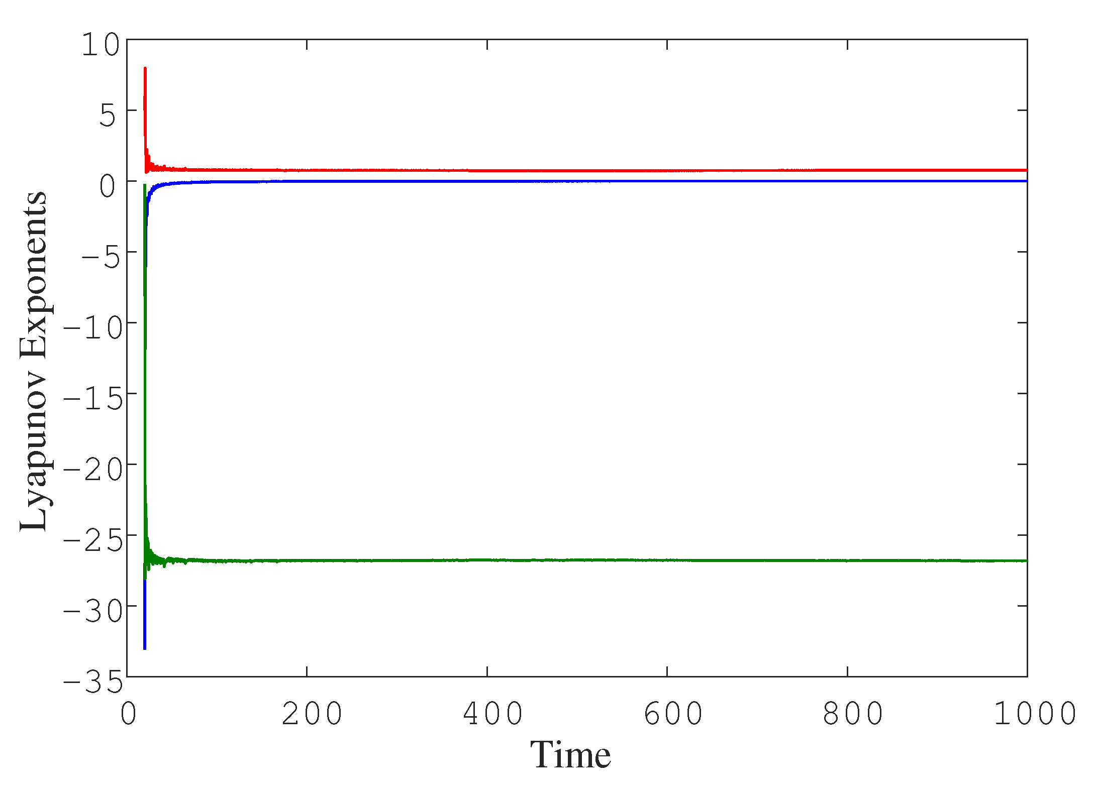
where and z are state variables, and a, b, c, and k are the control parameters. Note that adding a cross-product nonlinear term is not a general method to realize chaos in a 3D quadratic system. In addition, the proposed system (1) has three nonlinear terms, where notably each equation has one single cross-product term, so it certainly does not belong to algebraic simple chaotic flows, but is suitable for practical implementation as an electronic circuit. When the parameters of system (1) are assigned as and the initial values are set as , a fourth-order Runge–Kutta method is adopted in the numerical integration, which reveals the chaotic behaviors characterized by strange attractors, as shown in Figure 1a–c, and the power spectrum with continuous broadband characteristics (Figure 1d) verifies the emergence of chaos. Correspondingly, the Lyapunov exponents are calculated based on the Wolf algorithm [52], which gives (see Figure 2). The positive Lyapunov exponent indicates that the phase volume of the system is expanding and folding in a certain direction, which means that the system is in a chaotic state. The Kaplan–Yorke dimension is , which also verifies the chaoticity of system (1).
The new system has the following fundamental dynamic properties:
(1) System (1) is rotationally symmetric versus the z-axis, which is invariant under the coordinate transformation . Any attractors are either a symmetric pair or symmetric under a 180-degree rotation around the z-axis;
(2) Since the divergence of system (1) is
under the condition it is dissipative and can converge to a set of zero measure in exponential form,
(3) System (1) possesses two equilibrium points:
Linearizing the system gives the Jacobian matrix
For the parameters the Jacobian eigenvalues at and can be calculated by solving the corresponding characteristic equations, and they have the same values: From the eigenvalues, we can see that and are both stable node-focus points.
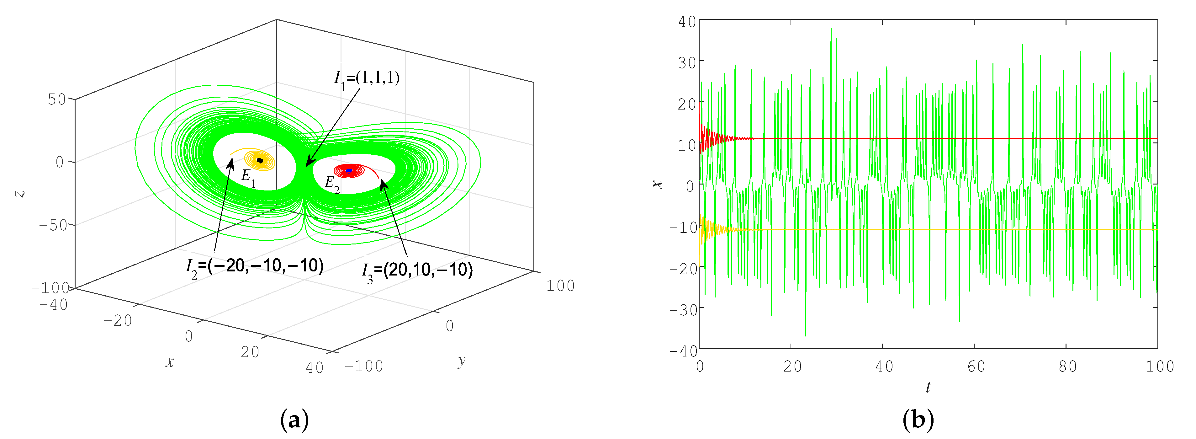
Since the new system can generate strange attractors, it is implied that system (1) under current parameters has hidden chaotic attractors. Figure 3a displays the coexistence of chaotic motion and stable node-foci in 3D phase space. We can see clearly that the trajectory starting from initial conditions becomes a disordered state; however, orbits starting from initial conditions and spirally converge to and , respectively. Figure 3b displays the time-domain waveform diagram for initial conditions , and ; an apparently chaotic waveform of illustrates that hidden chaotic attractors exist in system (1). To avoid transient chaos, we also confirmed the existence of a hidden chaotic attractor, since the orbit remains on it for .
The graphics of the basin of attraction, which is defined as the initial condition set that the orbits converge to a given attractor, can clearly exhibit the initial point distributions of different attractors. To further check whether the chaotic attractor in Figure 3 is hidden, a section , including and , is selected, and the initial condition regions of coexisting attractors are explored, as shown in Figure 4. Three types of basins of attraction on the cross section are colored yellow, blue, and red. Yellow areas with black stripes represent the basin of attraction of a chaotic attractor and the Poincaré section concerning the chaotic attractor with two wings, while blue and red areas denote that the movement from these initial conditions will converge to equilibria and , respectively. From Figure 4, we find that the basin of attraction has the expected symmetric similarity and a smooth boundary. Moreover, in view of the topology of basins in Figure 4, the basins of attraction of chaotic attractors do not intersect with small neighborhoods of stable equilibrium points and , which also illustrates that there is a hidden chaotic attractor in system (1).
3. Chaotic and Complex Dynamics in New System
The system parameters can significantly influence the dynamics, and the qualitative or topological variety in the behavior of dynamic systems means that a bifurcation occurs [53]. We discuss the chaotic and complex dynamics of the proposed system (1) through varying the parameters, taking the initial values as . The bifurcation diagram, largest Lyapunov exponent, and division diagram are adopted as tools to observe the impacts of parameters.
3.1. Fix and Vary b
To investigate the effect of the parameters on the dynamics of system (1), we first take parameters and vary . When altering b, the system shows many complex dynamic behaviors that can be explored in the parameter space. The typical Benettin method is employed to calculate the maximum Lyapunov exponent spectrum, and the corresponding bifurcation diagram versus parameter b is displayed in Figure 5. Obviously, a positive maximum Lyapunov exponent implies that the system is chaotic over a wide range of parameters. It is clear that the bifurcation diagram with the variation of parameter b matches well with the largest Lyapunov exponent spectrum. We can see that the state of system (1) becomes chaotic through pitchfork and period-doubling bifurcations, then periodic, and chaotic again. The bifurcation diagram in Figure 5b demonstrates that the system evolves smoothly from a periodic solution to a chaotic region through a typical period-doubling route; hence, no clear boundary exists between a periodic phase portrait and chaos. When b is in the interval , the largest Lyapunov exponent quickly becomes negative, and the corresponding bifurcation diagram suddenly changes to no cutoff points, which both mean that the trajectory of system (1) finally converges to a fixed point. More details are presented through the 3D projections of phase portraits of system (1) at different b values, as shown in Figure 6.
3.2. Fix and Vary a
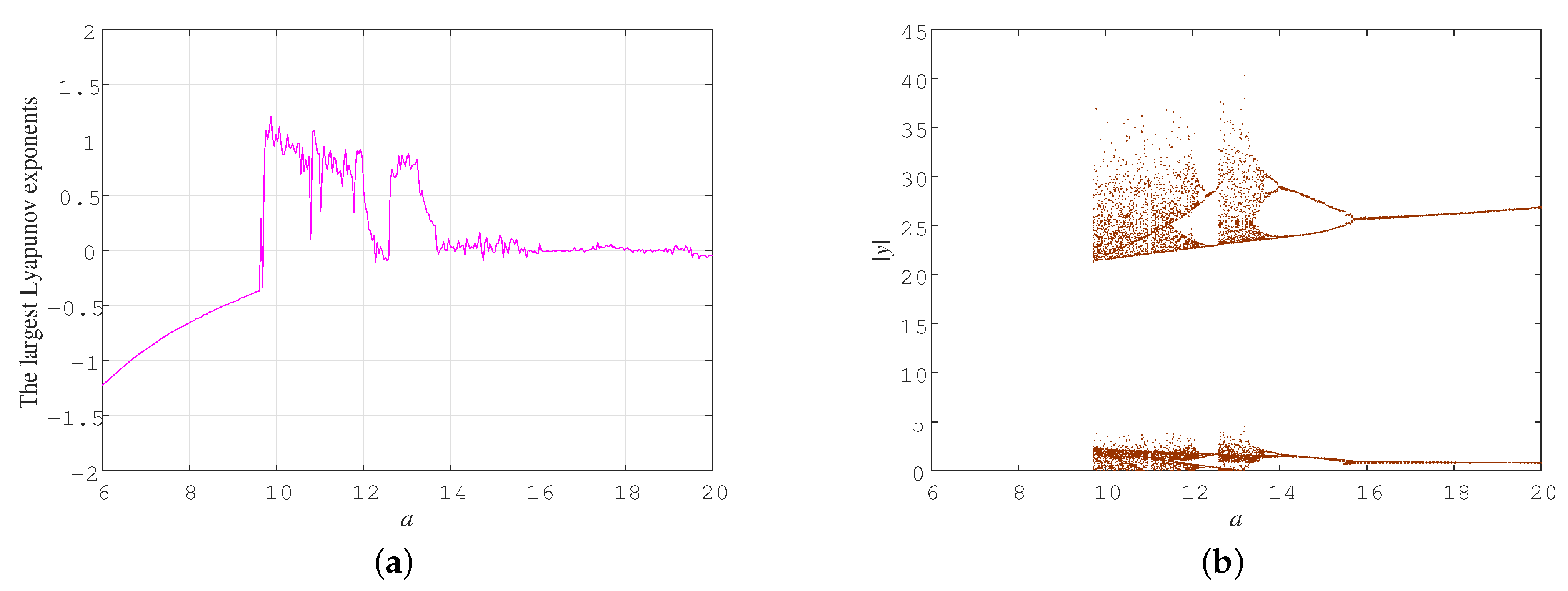
Now, we fix and vary and explore the dynamical evolution of system (1). Figure 7a shows the largest Lyapunov exponent spectrum with respect to a, and Figure 7b displays the bifurcation diagram of the whole evolution process. As can be seen from Figure 7, these results are consistent with each other and demonstrate that the dynamical behaviors vary when a undergoes change. Obviously, when a is in the interval , the system converges to one stable equilibrium, as shown in Figure 8a, where . When a, the system has a chaotic status. Near , the largest Lyapunov exponent is about zero, which implies that system (1) is periodic in a small parameter range, as demonstrated in Figure 8b, where However, the system becomes chaotic again when a is in the interval (see Figure 8c). Then, when , the system experiences an inverse period-doubling bifurcation process with the increase of a, and eventually becomes periodic again. Figure 8d displays the 3D phase diagram for .
3.3. Fix and Vary c
Here, we fix the parameters , and vary c. The Lyapunov exponent spectrum and bifurcation diagram presented in Figure 9 reveal that the limit cycle, chaos, and equilibrium point appear alternately as c increases from −30 to 20. We can see that the system shows complex dynamic behavior in this region, and generates chaos via period-doubling bifurcation. Moreover, periodic windows exist in such a parameter region. An attractor of system (1) becomes a limit cycle from chaos through a process of reverse period-doubling bifurcations, then becomes chaotic again through period-doubling bifurcations, and finally converges to a stable equilibrium point. With initial values , the system will undergo the same bifurcation process, and the orbits in the phase space will eventually converge toward another stable fixed point.
When the parameters , the emergence of a hidden chaotic attractor is dependent on the value of . When we take , the system generates a self-excited chaotic attractor. It is worth noting that the periodic regions do not share the same dynamical characteristics; diverse limit cycles appear in four periodic regions, as shown in Figure 10.
3.4. Fix and Vary k
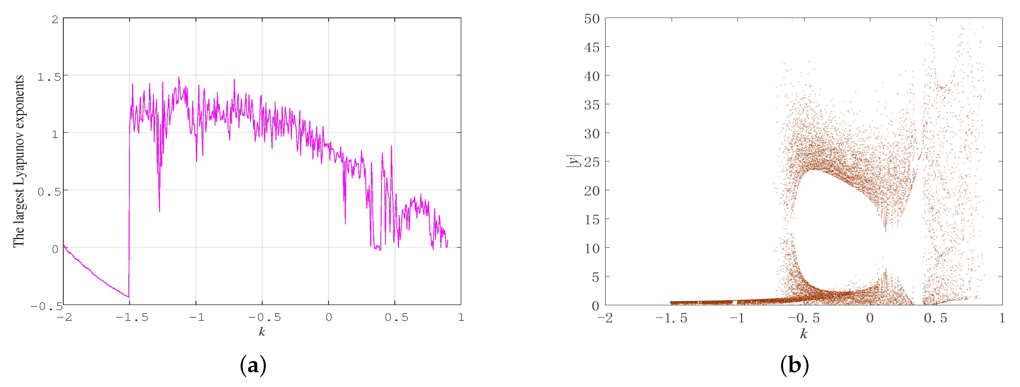
The Lyapunov exponent spectrum and bifurcation diagram shown in Figure 11 reveal that equilibrium point and chaotic orbit appear alternately with k increasing gradually from to . When we take parameters , system (1) becomes the system with a hidden chaotic attractor in Ref. [51]. As shown in Figure 11, when k becomes slightly positive or negative, chaotic attractors can still be generated. However, the type of chaotic attractors will depend on the positive or negative value of k; these are the new structures that have emerged. As required by the Routh–Hurwitz stability criterion, when we take parameters , hidden chaotic attractors can exist if the following inequalities are satisfied: , which requires or . Hence, when k is slightly positive, the chaotic attractor is self-excited, while when k is slightly negative, it generates a hidden chaotic attractor with two stable node-foci. It is noteworthy that, with k increasing in the range , the orbit finally leads to infinity.
3.5. Fix and Vary k and c
We draw a division diagram to capture different kinds of dynamical modes of system (1) with respect to parameters k–c. Varying k and c within the region of , , by calculating the largest Lyapunov exponents, we obtain a pseudo-colored map on a grid of parameters (see Figure 12a). Colors correspond to magnitudes of the largest Lyapunov exponents, where green and blue imply equilibrium, yellow indicates a limit cycle, and red represents a state of chaos. It can be observed from Figure 12a that the dynamical mode of system (1) evolves as k and c change. To more clearly show the evolution of chaos, we fix , take , and plot a vertical line A–B–C, presented in Figure 12a for . The rich dynamics of the evolution process in the division diagram are shown in Figure 9. Starting with the periodic region A, as c increases, the chaos degenerates through period-doubling bifurcations in line A–B, and the system abruptly changes to one equilibrium through the chaotic status in line B–C. Similarly, we plot a horizontal line, D–E, fix c at 11.2, and take . The system changes from one stable equilibrium to a chaotic state at .
Taking initial conditions , the numerical results in Figure 12b illustrate that the other initial conditions have an impact on the division diagram, leading to expansion of the regions of stable equilibrium. The original chaotic state regions become an equilibrium state, indicating the existence of a hidden attractor in the corresponding parameters. If the regions remain in a chaotic state, a self-excited attractor might exist under the corresponding parameters, as the regions may become one equilibrium at other initial values.
Inspired by the k–c division diagram, it is clear that the parameter values and at the lower-right corner are dark red, which means the chaos is most complex. As will be discussed shortly, system (1) has a self-excited chaotic attractor at parameter values .
4. Diverse Symbolic Dynamics for Unstable Periodic Orbits
We employ the variational method for the cycle search in system (1) and establish appropriate symbolic dynamics for the found periodic orbits. We first introduce the variational method, which can be effectively used in the calculations. After that, we aim to accurately find the surrounding mode of the orbit in system (1), and develop a universal approach for the symbolic encodings of cycles. We select two sets of parameters, one corresponding to the hidden chaotic attractor, and the other to the self-excited chaotic attractor. The symbolic encoding method based on orbit topology will enable us to analyze periodic orbits by establishing diverse symbolic dynamics.
As shown in Figure 1, the strange attractor of system (1) is composed of numerous unstable periodic orbits. The 3D continuous flow can be transformed to a 2D discrete mapping by an appropriate Poincaré section. The idea is to select a section properly in a high-dimensional phase space, on which a pair of conjugate variables are fixed; then, the information about the motion characteristics can be obtained by observing the intersection points of the motion trajectory and cross section. Figure 13a shows the first return map of system (1) for . When we choose a special Poincaré section , the initial values are where a dense point with a four-branch structure is presented under these parameters, which indicates the necessity to encode all short cycles by symbolic dynamics with four letters. For the parameters , which also correspond to a chaotic state, the first return map with a Poincaré section with the same initial values is shown in Figure 13b. We can see more branches in this case, which means that more symbols are needed to encode the periodic orbits, and demonstrates better complexity in the topological structure of periodic orbits. To the best of our knowledge, investigations of such complex unstable cycles in the chaotic attractor have rarely been reported. The Lyapunov exponents under the parameters are also calculated, which gives , , and (see Figure 14). Correspondingly, the Kaplan–Yorke dimension is . Compared with the largest Lyapunov exponent, i.e., 0.7457, under the parameters , the largest Lyapunov exponent becomes larger, which indicates that the chaotic characteristics of the system are more complex for the parameters .
4.1. Variational Method
Periodic orbits play important roles in physical and engineering applications. It is relatively easy to locate the unstable cycles in low-dimensional chaotic systems in general [54]. When we locate them in a high-dimensional state space, because the topological structure of the dynamical system is difficult to perceive, even if points on the cycle are guessed, the shooting method may fail. This problem can be solved by initializing a complete orbit with similar topology, and making it gradually evolve into a real cycle. This is also the basic idea for the variational method to calculate unstable periodic orbits of dynamical systems. For the calculations of unstable cycles, a discretization equation was derived as [55]
where is the virtual time related to iteration times. We use to adjust the period, which has the relationship with the period when the periodic orbit converges. We want to match the vector fields everywhere along the loop, and v and represent the flow velocity and loop velocity vector, respectively. is an -dimensional row vector that restricts coordinate alterations. where , is the gradient matrix of the velocity field, and the five-point approximation matrix is
where each matrix element is dimensional, and blanks are filled with zeros. The matrix on the left side of Equation (6) must be inverted to solve for and , and the banded lower-upper decomposition method for accelerated computing and the Woodbury formula are adopted. In addition, because the virtual time steps are sometimes not significant, we may choose larger time steps for numerical integration, so as to effectively search the real periodic orbit.
To utilize the variational method, as a first step, a loop guess which is fit to the cycle calculations is a prerequisite, and the loop guess can be initialized in many ways in the numerical calculations [55]. For example, we can use a fast Fourier transform of a nearly closed orbital fragment obtained from the numerical integration, keep only the lowest-frequency components, and use a reverse fast Fourier transform back to the phase space, in which emerges a glossy loop guess that can be used to initialize. We can also easily construct the initial loop guess by utilizing the homotopy evolution method [56]. We mention other initialization methods below.
The flexibility of the variational method for cycle searching has been verified by many examples [57,58,59], including conservative systems and low- or high-dimensional dissipative systems. The method can also locate other invariant sets in dynamical systems with proper modification [60,61]. The method cannot only find cycles with fixed parameters, but can be used to study the deformations of cycles when changing some parameters, i.e., to investigate the bifurcation behaviors of a dynamical system [62,63]. Hence, this approach can be used to study the generation or disappearance of periodic orbits and the change of cycle stability.
4.2. Unstable Cycles Embedded in Hidden Chaotic Attractor for
The unstable periodic orbits in system (1) when are investigated based on the variational method. In the process, establishing appropriate symbolic dynamics is important for locating all short cycles without missing any [64]. To obtain the topological shape of the periodic orbit to be calculated, we perform numerical simulations, intercepting part of the simple orbital fragment to construct the initial loop guess. Several short periodic orbits with uncomplicated topological structures are found, as shown in Figure 15. Figure 15a shows a periodic orbit that revolves one turn around the left equilibrium with an elliptical shape, which has a relatively small extension in the z-axis with shortest period We mark it as cycle 0. Figure 15b shows a cycle that rotates once around the right equilibrium with an elliptical shape, and mark it as cycle 1. It can be seen that the two periodic orbits are symmetric to each other. Similarly, we mark the cycle with a wing shape rotating around the fixed point on the left once as cycle 2, as shown in Figure 15c, and its symmetric cycle with reasonably large extension in the z orientation is denoted as cycle 3 (see Figure 15d). The above four cycles can be regarded as the building blocks, and other periodic orbits can be calculated systematically by the symbolic dynamics of four letters.
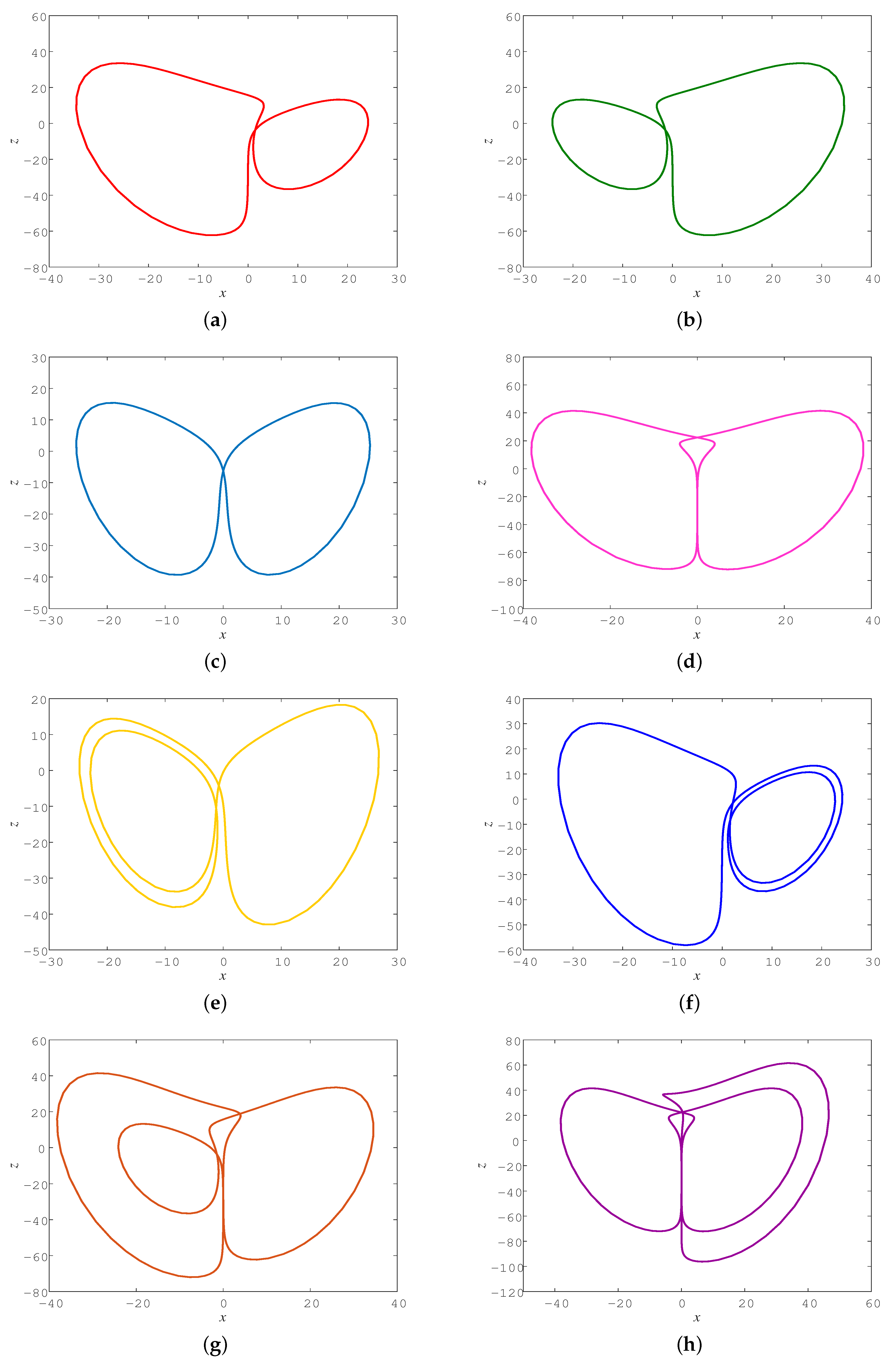
There are four situations in which an orbit revolves one turn both around the left and right fixed points, and they are the cycles with topological length 2, as listed in Figure 16a–d. The rotationally symmetric property of system (1) implies the exchange symmetry 0 and 1 or 2 and 3 of the symbol sequence. Consequently, it is shown that the symmetry partner of cycle 12 is 03, and they have the same period. Cycles 01 or 23 are conjugated with themselves, so that no other orbit has the same period. Figure 16e–h display four cycles with topological length 3. Utilizing symbolic dynamics, we can calculate the cycles up to any topological length, i.e., we first construct the loop guess of the corresponding symbol sequence, and use the variational technique to verify its existence. Altogether, we found 20 periodic orbits with topological length 3, as listed in Table 1.
4.3. Unstable Periodic Orbits Embedded in Self-Excited Chaotic Attractor for
If we make the third and fourth parameters in the chosen set zero, according to the Routh–Hurwitz stability criterion, must be satisfied, so there is no solution, which means that there will be no hidden chaotic attractors in the system. Only when c and k are not zero is it possible to satisfy the Routh–Hurwitz stability criterion and a hidden chaotic attractor with stable equilibrium points can exist. When we take another set of parameters, , system (1) becomes a dynamical system with only five terms and also exhibits the existence of a chaotic state. As with some simple chaotic flows, namely the Sprott system, listed in Ref. [15], system (1) is simpler, but it has more complex dynamics, which is worthy of further research. For these parameter values, the two equilibrium points yield and and three eigenvalues of the fixed points are and . Since are two saddle-foci, system (1) has a self-excited chaotic attractor under current parameters.
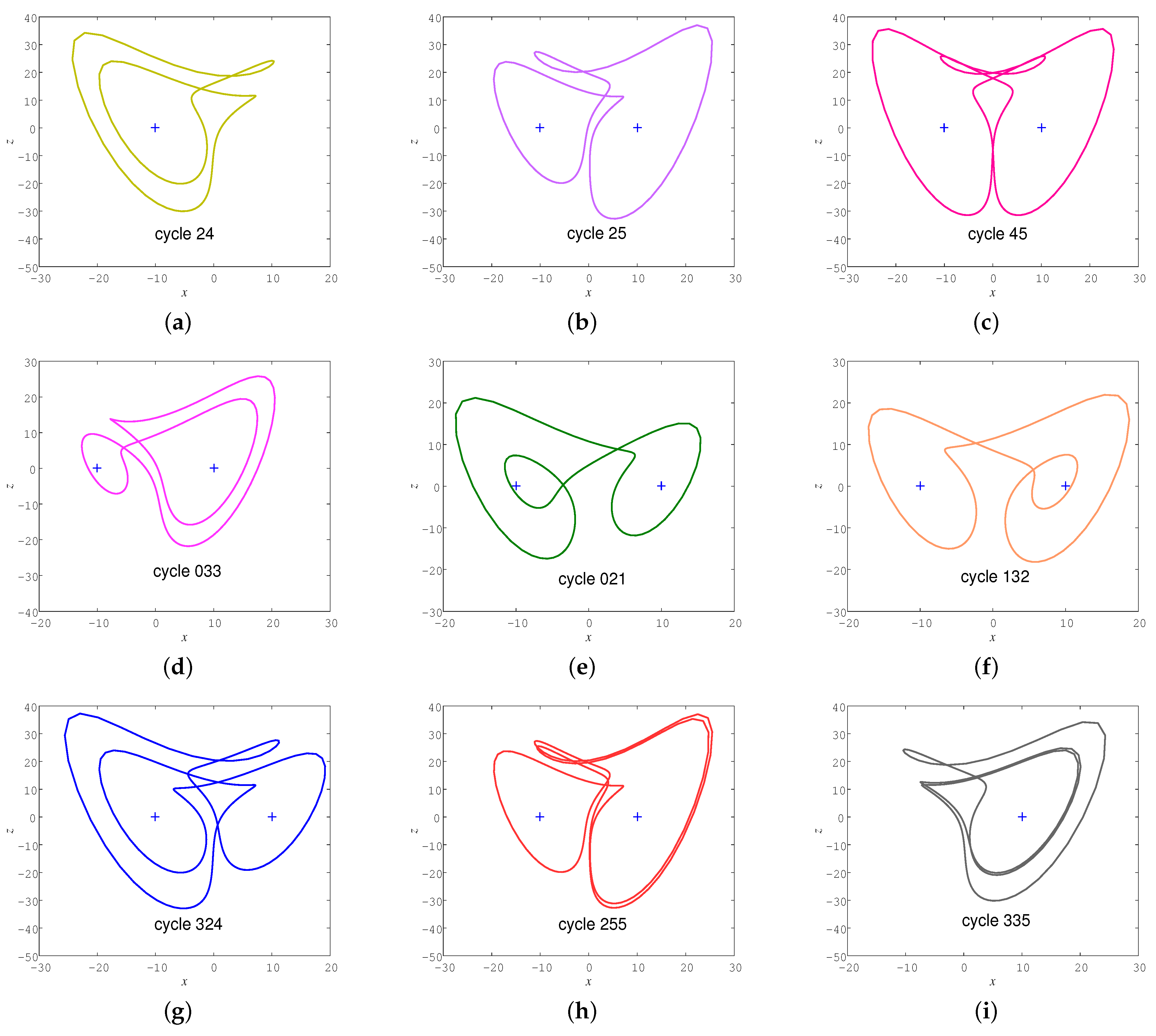
We locate the unstable periodic orbits via the variational method, which brings great convenience. Here, we numerically integrate Equation (1) and extract approximate closed trajectories with different shapes, then artificially connect them so as to initialize the search. Figure 17 displays our calculated results for some short periodic orbits. We can also record the cycle swirling around the left fixed point once with a wing shape in Figure 17a by cycle 2, and its symmetric partner in Figure 17b with cycle 3. However, we did not find cycle 0 and cycle 1 to exist. The cycles in Figure 17c,d both have a knot, which indicates that they have a self-linking number of 1, which can conveniently be calculated [65]. We mark them as cycle 4 and cycle 5, respectively. Noting that they are symmetric to each other, the commutative symmetry 4 and 5 of the symbol sequence is satisfied.
We can use the above cycles as building blocks to find more complicated cycles, and the symbolic dynamics is established successfully. Figure 18 shows part of the found cycles together with equilibria and . According to the symbolic dynamics, we find 41 unstable cycles with topological lengths up to 3, and sort them in Table 2. A total of 14 cycles are pruned, e.g., cycles 02, 002, and 123. Compared with the two sets of parameters, for the same periodic orbits, the cycles embedded in the hidden chaotic attractor have longer periods than those embedded in the self-excited chaotic attractor. The unstable cycles of system (1), as discussed under current parameters, must invoke symbolic dynamics for six letters, which is usually complicated. The topological classification approach used here indicates its flexibility. Additionally, although the symbolic dynamics of six letters can produce many symbol sequences within the topological length of 3, it is found that the 2 and 3 building blocks can be combined with all the other building blocks, while the 0 and 1 building blocks cannot be combined with the 4 or 5 building blocks. These behaviors are surely unusual. Therefore, the number of cycles actually allowed by the symbol sequence is greatly reduced. Whether this empirical pruning rule is applicable to longer periodic orbits is an open problem worthy of further investigation.
Regarding the system’s overall dynamical complexity from the two sets of parameters chosen in the study, we can draw the following conclusions:
(1) The proposed system (1) with two parameters has more complex dynamics than the system with four parameters.
(2) The system with a self-excited attractor has more complex dynamics than the system with a hidden attractor.
(3) The system with periodic orbits containing building blocks of self-linking number 1 has more complex dynamics than that containing building blocks of self-linking number 0.
5. Circuit Simulation
We discuss the circuit implementation of system (1) to confirm the realizability of the mathematical model. Because all the values of state variables in system (1) are out of the dynamic range, they should be scaled down to avoid problems during simulation. We set the amplitude scaling factor to 10, where , , and . The time scale factor is set to to better match the system, a new time variable is defined instead of t, and As a result, system (1) after scale transformation is described as
where and .
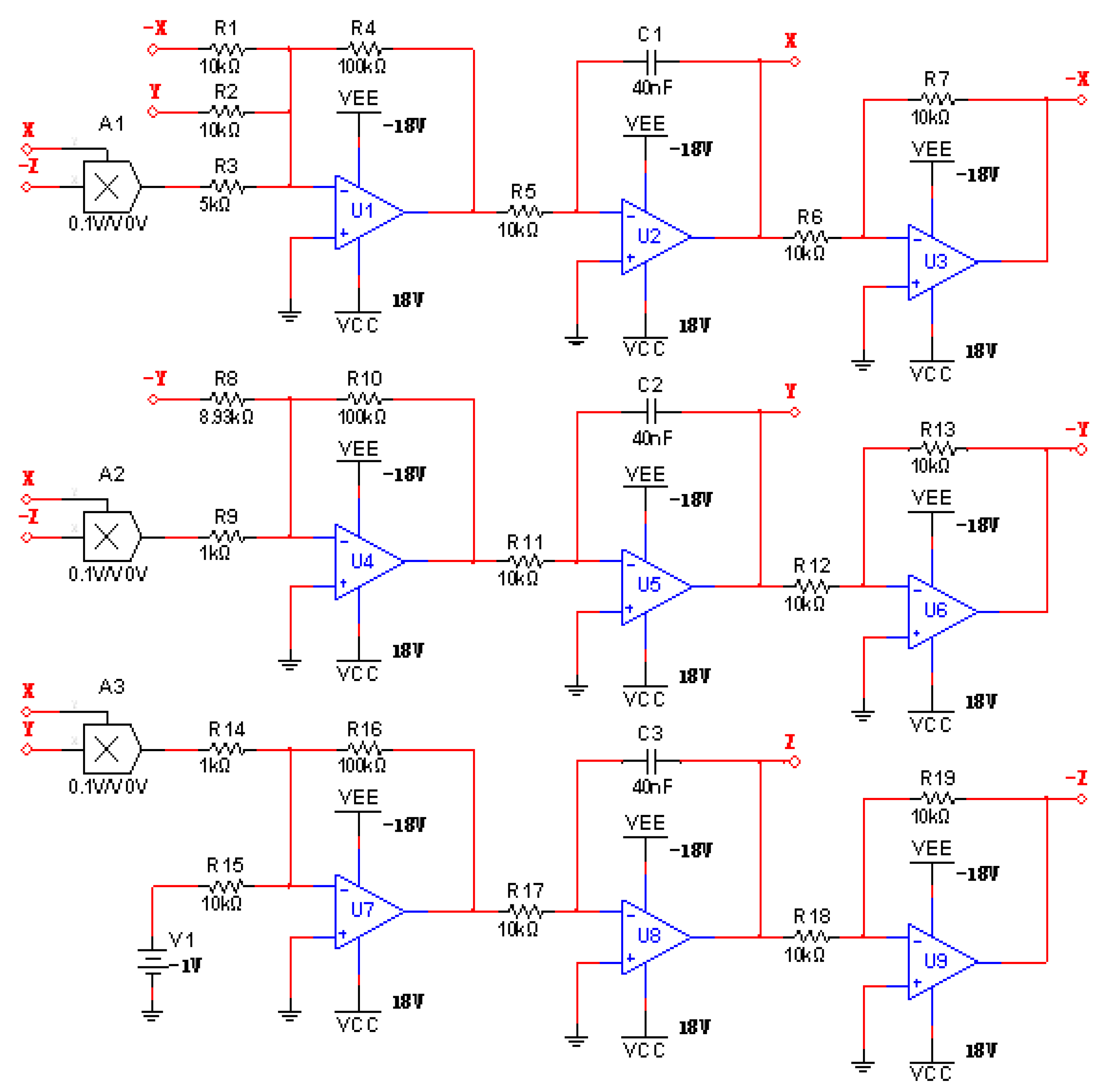
The proposed circuit design is depicted in Figure 19, in which X, Y, and Z are the voltages at the outputs of operational amplifiers U2, U5, and U8, respectively. The circuit consists of nine AD811AN operational amplifiers, whose supply voltage is ±18 V; three multipliers with an output coefficient of 0.1; three capacitors; and 19 resistors. Based on Kirchhoff’s law, we can get
Comparing Equation (8) with Equation (9), we select all the capacitors = 40 nF and = −1 V. The resistors = 1 kΩ, = 5 kΩ, = 8.93 kΩ, = 10 kΩ , and = 100 kΩ We used NI Multisim 14.0 to simulate the circuit, as shown in Figure 20. It can be seen that the circuit well emulates the proposed system, which is in good agreement with the numerical results in Figure 1. Therefore, we can conclude that system (1) can be realized in physical experiments.
6. Conclusions and Discussion
We constructed a new 3D autonomous chaotic system with coexisting self-excited and hidden attractors, in which the generation of different types of attractors depends on its parameters. The complex dynamics of the system were analyzed by different tools, and it was proved to be chaotic in the sense of having a fractional Kaplan–Yorke dimension, a phase portrait of a strange attractor, and a period-doubling route to chaos. Moreover, an applicable generic procedure for topological classification of unstable cycles in the proposed system was addressed. Guessing an entire orbit, we utilized the variational method for the calculation of cycles, and the initial conjecture loop could be gradually evolved into a real cycle. Diverse symbolic dynamics based on orbital topology was successfully established in the phase space, including four and six letters, corresponding to hidden and self-excited chaotic attractors. Periodic orbits up to certain topological lengths were found accordingly, which indicates the utility of the topological classification approach in the periodic orbit taxonomy. A Multisim circuit simulation of the system was implemented to further verify the mathematical model.
The symbolic encoding method employed here could also be applied to discrete dynamical systems, such as the memristive Rulkov neuron model [66], discrete memristor hyperchaotic maps [67], 2D memristive hyperchaotic maps [68], and 2D sine map [69]. Quotienting symmetries of a given dynamical system prior to the symbolic dynamics analysis is an attractive research direction. Symmetry reduction could not only reduce the multiple-letter symbolic encodings of periodic orbits to a single letter, but could visualize self-linking in the symmetry-reduced state space, which requires further investigation. The new system still contains rich and complex dynamic behavior, and its topology requires comprehensive and deep exploration. Moreover, as the system proposed in Ref. [51], the newly proposed system (1) is a mathematical model at present and does not correspond to any physical phenomena. It is hoped that more detailed theoretical analysis and application investigations will be carried out in the future.
Funding
This research was funded by National Natural Science Foundation of China (Grant Nos. 11647085 and 11647086), Shanxi Province Science Foundation for Youths (Grant No. 201901D211252), and the Scientific and Technological Innovation Programs of Higher Education Institutions in Shanxi (Grant Nos. 2019L0505 and 2019L0554).
Institutional Review Board Statement
Not applicable.
Informed Consent Statement
Not applicable.
Data Availability Statement
Not applicable.
Acknowledgments
I thank the anonymous reviewers for their many insightful comments and suggestions, which have improved our manuscript substantially.
Conflicts of Interest
The author declares no conflict of interest.
References
- Lorenz, E.N. Deterministic nonperiodic flow. J. Atmos. Sci. 1963, 20, 130–141. [Google Scholar] [CrossRef] [Green Version]
- Fu, S.; Liu, Y.; Ma, H.; Du, Y. Control chaos to different stable states for a piecewise linear circuit system by a simple linear control. Chaos Solitons Fractals 2020, 130, 109431. [Google Scholar] [CrossRef]
- Gong, L.H.; Luo, H.X.; Wu, R.Q.; Zhou, N.R. New 4D chaotic system with hidden attractors and self-excited attractors and its application in image encryption based on RNG. Physica A 2022, 591, 126793. [Google Scholar] [CrossRef]
- Hassan, M.F. Synchronization of uncertain constrained hyperchaotic systems and chaos-based secure communications via a novel decomposed nonlinear stochastic estimator. Nonlinear Dyn. 2016, 83, 2183–2211. [Google Scholar] [CrossRef]
- Sangiorgio, M.; Dercole, F. Robustness of lstm neural networks for multi-step forecasting of chaotic time series. Chaos Solitons Fractals 2020, 139, 110045. [Google Scholar] [CrossRef]
- Zhou, L.; You, Z.; Tang, Y. A new chaotic system with nested coexisting multiple attractors and riddled basins. Chaos Solitons Fractals 2021, 148, 111057. [Google Scholar] [CrossRef]
- Nwachioma, C.; Pérez-Cruz, J.H. Analysis of a new chaotic system, electronic realization and use in navigation of differential drive mobile robot. Chaos Solitons Fractals 2021, 144, 110684. [Google Scholar] [CrossRef]
- Wang, G.; Yuan, F.; Chen, G.; Zhang, Y. Coexisting multiple attractors and riddled basins of a memristive system. Chaos 2018, 28, 013125. [Google Scholar] [CrossRef]
- Ly, A.; Qy, A.; Gc, B. Hidden attractors, singularly degenerate heteroclinic orbits, multistability and physical realization of a new 6D hyperchaotic system. Commun. Nonlinear Sci. Numer. Simul. 2020, 90, 105362. [Google Scholar]
- Dudkowski, D.; Jafari, S.; Kapitaniak, T.; Kuznetsov, N.V.; Leonov, G.A.; Prasad, A. Hidden attractors in dynamical systems. Phy. Rep. 2016, 637, 1–50. [Google Scholar] [CrossRef]
- Jafari, S.; Sprott, J.C.; Nazarimehr, F. Recent new examples of hidden attractors. Eur. Phys. J. Spec. Top. 2015, 224, 1469–1476. [Google Scholar] [CrossRef]
- Pham, V.T.; Kapitaniak, T.; Volos, C. Systems with Hidden Attractors: From Theory to Realization in Circuits; Springer: Berlin, Germany, 2017; pp. 11–13. [Google Scholar]
- Chen, G.R.; Ueta, T. Yet another chaotic attractor. Int. J. Bifurc. Chaos 1999, 9, 1465–1466. [Google Scholar] [CrossRef]
- Qi, G.; Chen, G.; Du, S.; Chen, Z.; Yuan, Z. Analysis of a new chaotic system. Physica A 2005, 352, 295–308. [Google Scholar] [CrossRef]
- Sprott, J.C. Some simple chaotic flows. Phys. Rev. E 1994, 50, 647–650. [Google Scholar] [CrossRef] [PubMed]
- Guan, X.; Xie, Y. Connecting curve: A new tool for locating hidden attractors. Chaos 2021, 31, 113143. [Google Scholar] [CrossRef] [PubMed]
- Kuznetsov, N.V.; Leonov, G.A.; Mokaev, T.N.; Prasad, A.; Shrimali, M.D. Finite-time lyapunov dimension and hidden attractor of the rabinovich system. Nonlinear Dyn. 2018, 92, 267–285. [Google Scholar] [CrossRef] [Green Version]
- Deng, Q.; Wang, C. Multi-scroll hidden attractors with two stable equilibrium points. Chaos 2019, 29, 093112. [Google Scholar] [CrossRef] [PubMed]
- Yang, T. Multistability and hidden attractors in a three-dimensional chaotic system. Int. J. Bifurc. Chaos 2020, 30, 2050087. [Google Scholar] [CrossRef]
- Molaie, M.; Jafari, S.; Sprott, J.C.; Golpayegani, S.M.R.H. Simple chaotic flows with one stable equilibrium. Int. J. Bifurc. Chaos 2013, 23, 1350188. [Google Scholar] [CrossRef]
- Huang, L.; Wang, Y.; Jiang, Y.; Lei, T. A novel memristor chaotic system with a hidden attractor and multistability and its implementation in a circuit. Math. Probl. Eng. 2021, 2021, 7457220. [Google Scholar] [CrossRef]
- Wang, X.; Viet-Thanh, P.; Christos, V. Dynamics, circuit design, and synchronization of a new chaotic system with closed curve equilibrium. Complexity 2017, 2017, 7138971. [Google Scholar] [CrossRef] [Green Version]
- Jafari, S.; Sprott, J.C.; Pham, V.T.; Volos, C.; Li, C. Simple chaotic 3d flows with surfaces of equilibria. Nonlinear Dyn. 2016, 86, 1349–1358. [Google Scholar] [CrossRef]
- Zhang, X.; Tian, Z.; Li, J.; Wu, X.; Cui, Z. A hidden chaotic system with multiple attractors. Entropy 2021, 23, 1341. [Google Scholar] [CrossRef] [PubMed]
- Li, C.; Sprott, J.C. Coexisting hidden attractors in a 4-D simplified lorenz system. Int. J. Bifurc. Chaos 2014, 24, 1450034. [Google Scholar] [CrossRef]
- Jafari, S.; Sprott, J.C.; Mohammad Reza Hashemi Golpayegani, S. Elementary quadratic chaotic flows with no equilibria. Phys. Lett. A 2013, 377, 699–702. [Google Scholar] [CrossRef]
- Zhou, W.; Wang, G.; Shen, Y.; Yuan, F.; Yu, S. Hidden coexisting attractors in a chaotic system without equilibrium point. Int. J. Bifurc. Chaos 2018, 28, 1830033. [Google Scholar] [CrossRef]
- Zuo, J.L.; Li, C.L. Multiple attractors and dynamic analysis of a no-equilibrium chaotic system. Optik 2016, 127, 7952–7957. [Google Scholar] [CrossRef]
- Maaita, J.O.; Volos, C.K.; Kyprianidis, I.M.; Stouboulos, I.N. The dynamics of a cubic nonlinear system with no equilibrium point. J. Nonlinear Dyn. 2015, 2015, 257923. [Google Scholar] [CrossRef] [Green Version]
- Sprott, J.C.; Jafari, S.; Pham, V.T.; Hosseinib, Z.S. A chaotic system with a single unstable node. Phys. Lett. A 2015, 379, 2030–2036. [Google Scholar] [CrossRef]
- Wang, X.; Chen, G.R. A chaotic system with only one stable equilibrium. Commun. Nonlinear Sci. Numer. Simul. 2012, 17, 1264–1272. [Google Scholar] [CrossRef] [Green Version]
- Wei, Z. Dynamical behaviors of a chaotic system with no equilibria. Phys. Lett. A 2011, 376, 102–108. [Google Scholar] [CrossRef]
- Yang, Y.; Huang, L.; Xiang, J.; Bao, H.; Li, H. Generating multi-wing hidden attractors with only stable node-foci via non-autonomous approach. Phys. Scr. 2021, 96, 125220. [Google Scholar] [CrossRef]
- Wei, Z.; Yang, Q. Dynamical analysis of the generalized sprott C system with only two stable equilibria. Nonlinear Dyn. 2012, 68, 543–554. [Google Scholar] [CrossRef]
- Tian, H.; Wang, Z.; Zhang, P.; Chen, M.; Wang, Y. Dynamic analysis and robust control of a chaotic system with hidden attractor. Complexity 2021, 2021, 8865522. [Google Scholar] [CrossRef]
- Wang, Z.; Sun, W.; Wei, Z.; Zhang, S. Dynamics and delayed feedback control for a 3D jerk system with hidden attractor. Nonlinear Dyn. 2015, 82, 577–588. [Google Scholar] [CrossRef]
- Wei, Z.; Zhang, W.; Yao, M. On the periodic orbit bifurcating from one single non-hyperbolic equilibrium in a chaotic jerk system. Nonlinear Dyn. 2015, 82, 1251–1258. [Google Scholar] [CrossRef]
- Qi, A.; Muhammad, K.; Liu, S. Dynamical analysis of the meminductor-based chaotic system with hidden attractor. Fractals 2021, 29, 2140020. [Google Scholar] [CrossRef]
- Wei, Z.; Zhang, W.; Wang, Z.; Yao, M. Hidden attractors and dynamical behaviors in an extended Rikitake system. Int. J. Bifurc. Chaos 2015, 25, 1550028. [Google Scholar] [CrossRef]
- Wei, Z.; Yu, P.; Zhang, W.; Yao, M. Study of hidden attractors, multiple limit cycles from Hopf bifurcation and boundedness of motion in the generalized hyperchaotic Rabinovich system. Nonlinear Dyn. 2015, 82, 131–141. [Google Scholar] [CrossRef]
- Wei, Z.; Zhang, W. Hidden hyperchaotic attractors in a modified Lorenz–Stenflo system with only one stable equilibrium. Int. J. Bifurc. Chaos 2014, 24, 1450127. [Google Scholar] [CrossRef]
- Wei, Z.; Moroz, I.; Sprott, J.C.; Akgul, A.; Zhang, W. Hidden hyperchaos and electronic circuit application in a 5D self-exciting homopolar disc dynamo. Chaos 2017, 27, 033101. [Google Scholar] [CrossRef] [PubMed] [Green Version]
- Wang, N.; Zhang, G.; Kuznetsov, N.V.; Bao, H. Hidden attractors and multistability in a modified Chua’s circuit. Commun. Nonlinear Sci. Numer. Simul. 2021, 92, 105494. [Google Scholar] [CrossRef]
- Bao, H.; Hu, A.; Liu, W.; Bao, B. Hidden bursting firings and bifurcation mechanisms in memristive neuron model with threshold electromagnetic induction. IEEE Trans. Neural Netw. Learn. Syst. 2020, 31, 502–511. [Google Scholar] [CrossRef] [PubMed]
- Wu, Y.; Wang, C.; Deng, Q. A new 3d multi-scroll chaotic system generated with three types of hidden attractors. Eur. Phys. J. Spec. Top. 2021, 230, 1863–1871. [Google Scholar] [CrossRef]
- Wei, Z.; Li, Y.; Sang, B.; Liu, Y.; Zhang, W. Complex dynamical behaviors in a 3D simple chaotic flow with 3D stable or 3D unstable manifolds of a single equilibrium. Int. J. Bifurc. Chaos 2019, 29, 1950095. [Google Scholar] [CrossRef]
- Kingni, S.T.; Jafari, S.; Pham, V.T.; Woafo, P. Constructing and analyzing of a unique three-dimensional chaotic autonomous system exhibiting three families of hidden attractors. Math. Comput. Simul. 2017, 132, 172–182. [Google Scholar] [CrossRef]
- Zhang, S.; Zeng, Y.; Li, Z.; Wang, M.; Le, X. Generating one to four-wing hidden attractors in a novel 4D no-equilibrium chaotic system with extreme multistability. Chaos 2018, 28, 013113. [Google Scholar] [CrossRef] [PubMed]
- Jafari, S.; Ahmadi, A.; Khalaf, A.; Abdolmohammadi, H.R.; Pham, V.T.; Alsaadi, F.E. A new hidden chaotic attractor with extreme multi-stability. AEU—Int. J. Electron. C. 2018, 89, 131–135. [Google Scholar] [CrossRef]
- Cang, S.; Yue, L.; Zhang, R.; Wang, Z. Hidden and self-excited coexisting attractors in a lorenz-like system with two equilibrium points. Nonlinear Dyn. 2019, 95, 381–390. [Google Scholar] [CrossRef]
- Yang, Q.; Wei, Z.; Chen, G. An unusual 3d autonomous quadratic chaotic system with two stable node-foci. Int. J. Bifurc. Chaos 2010, 20, 1061–1083. [Google Scholar] [CrossRef]
- Wolf, A.; Swift, J.B.; Swinney, H.L.; Vastano, J.A. Determining Lyapunov exponents from a time series. Physica D 1985, 16, 285–317. [Google Scholar] [CrossRef] [Green Version]
- Strogatz, S.H. Nonlinear Dynamics and Chaos: With Applications to Physics, Biology, Chemistry, and Engineering; Perseus Books: Reading, MA, USA, 1994; pp. 44–45. [Google Scholar]
- Cvitanović, P.; Artuso, R.; Mainieri, R.; Tanner, G.; Vattay, G. Chaos: Classical and Quantum; Niels Bohr Institute: Copenhagen, Denmark, 2012; pp. 131–133. [Google Scholar]
- Lan, Y.; Cvitanović, P. Variational method for finding periodic orbits in a general flow. Phys. Rev. E 2004, 69, 016217. [Google Scholar] [CrossRef] [Green Version]
- Dong, C.; Jia, L.; Jie, Q.; Li, H. Symbolic encoding of periodic orbits and chaos in the Rucklidge system. Complexity 2021, 2021, 4465151. [Google Scholar] [CrossRef]
- Lan, Y.; Cvitanović, P. Unstable recurrent patterns in Kuramoto–Sivashinsky dynamics. Phys. Rev. E 2008, 78, 026208. [Google Scholar] [CrossRef] [PubMed] [Green Version]
- Dong, C.; Liu, H.; Li, H. Unstable periodic orbits analysis in the generalized Lorenz-type system. J. Stat. Mech. 2020, 2020, 073211. [Google Scholar] [CrossRef]
- Dong, C. Topological classification of periodic orbits in the kuramoto–sivashinsky equation. Mod. Phys. Lett. B 2018, 32, 1850155. [Google Scholar] [CrossRef]
- Lan, Y.; Chandre, C.; Cvitanović, P. Newton’s descent method for the determination of invariant tori. Phys. Rev. E 2006, 74, 046206. [Google Scholar] [CrossRef] [Green Version]
- Dong, C.; Lan, Y. A variational approach to connecting orbits in nonlinear dynamical systems. Phys. Lett. A 2014, 378, 705–712. [Google Scholar] [CrossRef]
- Dong, C.; Lan, Y. Organization of spatially periodic solutions of the steady Kuramoto–Sivashinsky equation. Commun. Nonlinear Sci. Numer. Simul. 2014, 19, 2140–2153. [Google Scholar] [CrossRef]
- Dong, C.; Liu, H.; Jie, Q.; Li, H. Topological classification of periodic orbits in the generalized Lorenz-type system with diverse symbolic dynamics. Chaos Solitons Fractals 2022, 154, 111686. [Google Scholar] [CrossRef]
- Hao, B.L.; Zheng, W.M. Applied Symbolic Dynamics and Chaos; World Scientic: Singapore, 1998; pp. 11–13. [Google Scholar]
- Ray, A.; Ghosh, D.; Chowdhury, A.R. Topological study of multiple coexisting attractors in a nonlinear system. J. Phys. A-Math. Theor. 2009, 42, 385102. [Google Scholar] [CrossRef]
- Li, K.; Bao, H.; Li, H.; Ma, J.; Hua, Z.; Bao, B. Memristive Rulkov neuron model with magnetic induction effects. IEEE Trans. Ind. Inform. 2022, 18, 1726–1736. [Google Scholar] [CrossRef]
- Bao, H.; Hua, Z.; Li, H.; Chen, M.; Bao, B. Discrete memristor hyperchaotic maps. IEEE Trans. Circuits—I 2021, 68, 4534–4544. [Google Scholar] [CrossRef]
- Li, H.; Hua, Z.; Bao, H.; Zhu, L.; Chen, M.; Bao, B. Two-dimensional memristive hyperchaotic maps and application in secure communication. IEEE Trans. Ind. Electron. 2021, 68, 9931–9940. [Google Scholar] [CrossRef]
- Bao, H.; Hua, Z.; Wang, N.; Zhu, L.; Chen, M.; Bao, B. Initials-boosted coexisting chaos in a 2-D Sine map and its hardware implementation. IEEE Trans. Ind. Inform. 2021, 17, 1132–1140. [Google Scholar] [CrossRef]
Figure 1.
Projections of chaotic attractor onto various planes at time : (a) x–z phase space; (b) y–z phase space; (c) x–y phase space; (d) continuous broadband frequency spectrum.
Figure 1.
Projections of chaotic attractor onto various planes at time : (a) x–z phase space; (b) y–z phase space; (c) x–y phase space; (d) continuous broadband frequency spectrum.

Figure 2.
Lyapunov exponent spectrum of system (1) for .

Figure 3.
(a) 3D phase portrait of system (1) for . Initial conditions lead to hidden chaotic attractor, and initial conditions lead to asymptotically converging behaviors to equilibrium point and respectively; (b) coexisting time series diagram of .
Figure 3.
(a) 3D phase portrait of system (1) for . Initial conditions lead to hidden chaotic attractor, and initial conditions lead to asymptotically converging behaviors to equilibrium point and respectively; (b) coexisting time series diagram of .

Figure 4.
Basins of attraction for system (1) at . Blue and red basins represent attractors of two stable node-focus points and , yellow region denotes basin of chaotic attractor, and black stripes denote crossing trajectories of chaotic attractor.
Figure 4.
Basins of attraction for system (1) at . Blue and red basins represent attractors of two stable node-focus points and , yellow region denotes basin of chaotic attractor, and black stripes denote crossing trajectories of chaotic attractor.

Figure 5.
Largest Lyapunov exponent spectrum (a) and bifurcation diagram (b) of system (1) versus b, where .
Figure 5.
Largest Lyapunov exponent spectrum (a) and bifurcation diagram (b) of system (1) versus b, where .

Figure 6.
3D view of phase portraits of system (1), where : (a) , (b) , (c) .


Figure 7.
Parameter values , largest Lyapunov exponent spectrum (a), and bifurcation diagram (b) of system (1) for .
Figure 7.
Parameter values , largest Lyapunov exponent spectrum (a), and bifurcation diagram (b) of system (1) for .

Figure 8.
3D view of phase portraits of system (1), : (a) ; (b) ; (c) ; (d) .

Figure 9.
Parameter values , largest Lyapunov exponent spectrum (a) and bifurcation diagram (b) of system (1) for .
Figure 9.
Parameter values , largest Lyapunov exponent spectrum (a) and bifurcation diagram (b) of system (1) for .

Figure 10.
2D view of different limit cycles of system (1), : (a) ; (b) ; (c) ; and (d) .

Figure 11.
Largest Lyapunov exponent spectrum (a) and bifurcation diagram (b) of system (1) versus k, where .
Figure 11.
Largest Lyapunov exponent spectrum (a) and bifurcation diagram (b) of system (1) versus k, where .

Figure 12.
Division of parameters k and c with different initial conditions: (a) (b) .

Figure 13.
First return map of system (1) under different parameters: (a) Poincaré section , ; (b) Poincaré section , .
Figure 13.
First return map of system (1) under different parameters: (a) Poincaré section , ; (b) Poincaré section , .

Figure 14.
Lyapunov exponent spectrum of system (1) for .

Figure 15.
Four basic building blocks in system (1) for parameters : (a) cycle 0; (b) cycle 1; (c) cycle 2; and (d) cycle 3.
Figure 15.
Four basic building blocks in system (1) for parameters : (a) cycle 0; (b) cycle 1; (c) cycle 2; and (d) cycle 3.

Figure 16.
Unstable cycles in system (1) under parameters : (a) cycle 12; (b) 03; (c) 01; (d) 23; (e) 001; (f) 112; (g) 023; and (h) 233.
Figure 16.
Unstable cycles in system (1) under parameters : (a) cycle 12; (b) 03; (c) 01; (d) 23; (e) 001; (f) 112; (g) 023; and (h) 233.

Figure 17.
Four building blocks in system (1) for parameters : (a) cycle 2; (b) cycle 3; (c) cycle 4; (d) cycle 5.
Figure 17.
Four building blocks in system (1) for parameters : (a) cycle 2; (b) cycle 3; (c) cycle 4; (d) cycle 5.

Figure 18.
Unstable periodic orbits in system (1) for parameters . Two equilibria are marked with “+”. (a) cycle 24; (b) cycle 25; (c) cycle 45; (d) cycle 033; (e) cycle 021; (f) cycle 132; (g) cycle 324; (h) cycle 255; (i) cycle 335; (j) cycle 325; (k) cycle 225; (l) cycle 254.
Figure 18.
Unstable periodic orbits in system (1) for parameters . Two equilibria are marked with “+”. (a) cycle 24; (b) cycle 25; (c) cycle 45; (d) cycle 033; (e) cycle 021; (f) cycle 132; (g) cycle 324; (h) cycle 255; (i) cycle 335; (j) cycle 325; (k) cycle 225; (l) cycle 254.


Figure 19.
Schematic of circuit.

Figure 20.
Phase portraits in Multisim of circuit: (a) X–Z plane; (b) X–Y plane.


Table 1.
Twenty unstable periodic orbits embedded in hidden chaotic attractor of system (1) for , showing topological length, itinerary p, period , and three coordinates of a point on the periodic orbit.
Table 1.
Twenty unstable periodic orbits embedded in hidden chaotic attractor of system (1) for , showing topological length, itinerary p, period , and three coordinates of a point on the periodic orbit.
| Length | p | x | y | z | |
|---|---|---|---|---|---|
| 1 | 0 | 0.635920 | −7.028076 | 0.430355 | 1.092913 |
| 1 | 0.635920 | 7.028076 | −0.430355 | 1.092913 | |
| 2 | 1.192933 | 2.544434 | 12.123766 | 20.650672 | |
| 3 | 1.192933 | −2.544434 | −12.123766 | 20.650672 | |
| 2 | 12 | 1.752388 | 2.807407 | 6.313538 | 12.146665 |
| 03 | 1.752388 | −2.807407 | −6.313538 | 12.146665 | |
| 01 | 1.467965 | 0.100280 | 1.271667 | −7.073590 | |
| 23 | 2.383824 | −14.090307 | 17.922194 | 33.086632 | |
| 3 | 001 | 2.174153 | −7.214950 | 4.081725 | 7.082844 |
| 011 | 2.174153 | 7.214950 | −4.081725 | 7.082844 | |
| 003 | 2.361334 | −1.162938 | −0.669254 | −14.983886 | |
| 112 | 2.361334 | 1.162938 | 0.669254 | −14.983886 | |
| 132 | 2.940945 | −2.570910 | −0.291669 | 11.591391 | |
| 023 | 2.940945 | 2.570910 | 0.291669 | 11.591391 | |
| 021 | 2.554559 | −0.016908 | −0.016629 | −31.681837 | |
| 013 | 2.554559 | 0.016908 | 0.016629 | −31.681837 | |
| 033 | 2.946229 | 0.291076 | 0.540818 | −60.155264 | |
| 122 | 2.946229 | −0.291076 | −0.540818 | −60.155264 | |
| 223 | 3.954898 | −5.509519 | −11.111451076 | −71.906347 | |
| 233 | 3.954898 | 5.509519 | 11.111451076 | −71.906347 |
Table 2.
Forty-one unstable periodic orbits embedded in self-excited chaotic attractor of system (1) for .
Table 2.
Forty-one unstable periodic orbits embedded in self-excited chaotic attractor of system (1) for .
| Length | p | Self-Linking | Length | p | Self-Linking | p | Self-Linking | |||
|---|---|---|---|---|---|---|---|---|---|---|
| 1 | 2 | 1.016946 | 0 | 3 | 223 | 2.994130 | 0 | 031 | 2.447450 | 2 |
| 3 | 1.016946 | 0 | 233 | 2.994130 | 0 | 012 | 2.447450 | 2 | ||
| 2 | 01 | 1.358438 | 1 | 033 | 2.609712 | 2 | 132 | 2.505368 | 0 | |
| 23 | 1.965825 | 1 | 122 | 2.609712 | 2 | 023 | 2.505368 | 0 | ||
| 12 | 1.587528 | 1 | 021 | 2.323226 | 0 | |||||
| 03 | 1.587528 | 1 | 013 | 2.323226 | 0 | |||||
| 1 | 4 | 1.312552 | 1 | 445 | 4.235720 | 3 | 354 | 3.955079 | 2 | |
| 5 | 1.312552 | 1 | 455 | 4.235720 | 3 | 234 | 3.263831 | 1 | ||
| 2 | 24 | 2.289914 | 2 | 344 | 3.667897 | 1 | 325 | 3.263831 | 1 | |
| 25 | 2.354458 | 0 | 255 | 3.667897 | 1 | 225 | 3.367249 | 1 | ||
| 34 | 2.354458 | 0 | 335 | 3.312270 | 1 | 334 | 3.367249 | 1 | ||
| 35 | 2.289914 | 2 | 224 | 3.312270 | 1 | 254 | 3.606269 | 3 | ||
| 45 | 2.642183 | 1 | 244 | 3.600833 | 3 | 345 | 3.606269 | 3 | ||
| 3 | 235 | 3.349139 | 1 | 355 | 3.600833 | 3 | ||||
| 324 | 3.349139 | 1 | 245 | 3.955079 | 2 |
Publisher’s Note: MDPI stays neutral with regard to jurisdictional claims in published maps and institutional affiliations. |
© 2022 by the author. Licensee MDPI, Basel, Switzerland. This article is an open access article distributed under the terms and conditions of the Creative Commons Attribution (CC BY) license (https://creativecommons.org/licenses/by/4.0/).
Share and Cite
MDPI and ACS Style
Dong, C. Dynamics, Periodic Orbit Analysis, and Circuit Implementation of a New Chaotic System with Hidden Attractor. Fractal Fract. 2022, 6, 190. https://doi.org/10.3390/fractalfract6040190
AMA Style
Dong C. Dynamics, Periodic Orbit Analysis, and Circuit Implementation of a New Chaotic System with Hidden Attractor. Fractal and Fractional. 2022; 6(4):190. https://doi.org/10.3390/fractalfract6040190
Chicago/Turabian StyleDong, Chengwei. 2022. "Dynamics, Periodic Orbit Analysis, and Circuit Implementation of a New Chaotic System with Hidden Attractor" Fractal and Fractional 6, no. 4: 190. https://doi.org/10.3390/fractalfract6040190