
Spatially Disaggregated Car Ownership Prediction Using Deep Neural Networks


1
Environmental Change Institute, University of Oxford, South Parks Road, Oxford OX1 3QY, UK
2
Institute for Energy & Environment, University of Strathclyde, 99 George Street, Glasgow G1 1RD, UK
3
Institute for Transport Studies, University of Leeds, 34-40 University Road, Leeds LS2 9JT, UK
*
Author to whom correspondence should be addressed.
Future Transp. 2021, 1(1), 113-133; https://doi.org/10.3390/futuretransp1010008
Submission received: 20 April 2021
/
Revised: 4 June 2021
/
Accepted: 15 June 2021
/
Published: 20 June 2021
Abstract
:Predicting car ownership patterns at high spatial resolution is key to understanding pathways for decarbonisation—via electrification and demand reduction—of the private vehicle fleet. As the factors widely understood to influence car ownership are highly interdependent, linearised regression models, which dominate previous work on spatially explicit car ownership modelling in the UK, have shortcomings in accurately predicting the relationship. This paper presents predictions of spatially disaggregated car ownership—and change in car ownership over time—in Great Britain (GB) using deep neural networks (NNs) with hyperparameter tuning. The inputs to the models are demographic, socio-economic and geographic datasets compiled at the level of Census Lower Super Output Areas (LSOAs)—areas covering between 300 and 600 households. It was found that when optimal hyperparameters are selected, these neural networks can predict car ownership with a mean absolute error of up to 29% lower than when formulating the same problem as a linear regression; the results from NN regression are also shown to outperform three other artificial intelligence (AI)-based methods: random forest, stochastic gradient descent and support vector regression. The methods presented in this paper could enhance the capability of transport/energy modelling frameworks in predicting the spatial distribution of vehicle fleets, particularly as demographics, socio-economics and the built environment—such as public transport availability and the provision of local amenities—evolve over time. A particularly relevant contribution of this method is that by coupling it with a technology dissipation model, it could be used to explore the possible effects of changing policy, behaviour and socio-economics on uptake pathways for electric vehicles —cited as a vital technology for meeting Net Zero greenhouse gas emissions by 2050.
1. Introduction
Surface transport is the largest contributing sector to UK greenhouse gas emissions, of which private cars make up the dominant share [1]. In their legally-binding commitment to reach Net Zero greenhouse gas emissions by 2050 [2], the UK Government must reduce surface transport emissions by 98%, from 116 MtCO2e/year in 2019 to 2 MtCO2 in 2050, according to the Climate Change Committee (CCC)’s Further Ambition scenario [3]. Much of this abatement will come from banning the sale of pure internal combustion engine vehicles from 2030—with the sale of plug-in hybrids banned from 2035 [4]. Given that (as of June 2021) battery electric vehicle (EV) sales contribute just 7% of total car sales [5], the rate of increase in EV adoption over the next fourteen years will need to accelerate significantly, assuming that the current market dominance of battery EVs over other low-emission-vehicle technologies (e.g., hydrogen fuel cell EVs) [6] will continue.
Wider transport system decarbonisation, however, requires more than a switch from internal combustion-powered vehicles to EVs. As part of the pathways released in their 2020 Sixth Carbon Budget recommendation, the CCC states that car miles per person must decrease by 17% from 2020 to 2050 [7] for the UK to meet Net Zero targets. Likewise, all three Net Zero-compatible pathways in National Grid ESO’s 2020 Future Energy Scenarios [8] show a decline in car ownership in the late-2030s to mid-2040s as private car travel is curbed in favour of increased public transport and active travel—which has been shown to be effective at replacing car-based trips and abating transport emissions [9]. Therefore, the characterisation of the relationship between demographics, socio-economics and the built environment (including public transport availability) to the spatial distribution of car ownership is an urgent area of research. By establishing which of these independent variables can be influenced by transport/energy policy, future pathways for car ownership—and hence technology shifts in the vehicle fleet—can be explored as a function of the changing policy, social and behavioural landscape. Furthermore, while it has long been predicted that EVs will present problems to electricity distribution networks with respect to their thermal and voltage limits [10,11,12,13,14], they also have the potential to interact positively with the grid—by providing flexible demand to utilise renewable generation when in surplus [15] and by charging bidirectionally to mitigate impacts on the network [16]. However, for these benefits to be realised, involved parties need to know where the EVs are likely to be at a given point in the future.
While car ownership modelling is a well-established field of the academic literature (Section 2), efforts to model the spatial distribution of car ownership have been few. Those that have attempted to do so in a UK context have used linear regression models, which are identified as problematic due to significant multicollinearity between the independent variables considered. To address these shortcomings, this paper presents a method of predicting the spatial variation in car ownership across Great Britain (GB) using an artificial neural network (NN) trained on key variables pertaining to these factors. A dataset of demographic, socio-economic and built environment variables is constructed from several sources (Table 1) for each of the three countries within GB (England, Wales and Scotland). NNs are designed and optimised using a hyperparameter tuning approach; once trained on the datasets, the predictions of car ownership are compared to those produced by an ordinary least squares (OLS) linear regression technique to highlight the benefit of this approach. Results are given for the base year of 2011 and for the prediction of the change in car ownership between 2001 and 2011. This approach can be used to predict future changes in the spatial distribution of vehicle ownership in GB. The spatial units of analysis in this paper are Lower Super Output Areas (LSOAs) for England & Wales, and analogous Data Zones (DZs) for Scotland—areas containing, on average, 672 and 340 households respectively.
2. Previous Work on Car Ownership Modelling
Car ownership is a major determinant of the modal split of the distance travelled by a population, and therefore car ownership forecasting is crucially important in transport system modelling [17]. Factors that influence car ownership are widely accepted to relate to household structure, socio-economic characteristics and the built environment (including the so-called ‘six Ds’ of diversity, density, design, destination accessibility, distance to transit, and demand management) [18,19,20].
Car ownership models can be broadly categorised into (i) longitudinal and (ii) cross-sectional. In longitudinal models, the evolution of car ownership is modelled year on year by considering the changing demand for cars. Such models generally follow a Sigmoid (S-shaped) curve, typical of the evolution of any technology, in which an initially slow rate of uptake increases to a steady linear rate of increase before plateauing at a quantity assumed to represent the saturation of car ownership. This approach is used in the UK Department for Transport’s National Car Ownership Model (NATCOP) [21] and the International Transport Forum’s 2019 car fleet model for France [22]. Conversely, cross-sectional models seek to predict car ownership at a point in time based on a snapshot of the explanatory variables, or changes in car ownership between two points in time based on changes in those variables between those points. Cross-sectional models have been employed as part of ‘pseudo-panel’ car ownership model (see for example [23]), which combines multiple cross-sectional datasets to predict the evolution in car ownership over time. Effectively, the model presented in this paper is a pseudo-panel model, in that multiple points in time are used to predict the change in car ownership over time. Whereas models in [21,22,23] predict changes in national car ownership (millions of vehicles), this paper is concerned with changes in car ownership per Census LSOA/DZ (hundreds of vehicles, scaled up to millions).
Prediction of car ownership given demographic, socio-economic and built environment variables are often based on forms of linear regression—either OLS, if the output of the model is treated as a discrete variable (the number of cars in a given area or owned by a given household), or logit, if the output is treated as a binary outcome (a household’s decision to buy another car or not). Either way, the prediction involves producing a line or curve of ‘best fit’ by iteratively estimating a set of coefficients in order to minimise the mean squared error (MSE) (in the case of OLS regression) or maximise the likelihood function (in the case of logit regression).
In [24], the authors present a study of the relationship between vehicle energy demand in GB and demographic, socio-economic and built environment variables using OLS linear regression, though clusters are first formed pertaining to the energy use of the households being studied. In [25], OLS linear regression is employed to quantify the relationship between CO2 emissions of private vehicle use with demographic, socio-economic and built environment variables. In [26], an OLS linear regression model is built to predict car ownership in China with a focus on geospatial built environment variables (e.g., the ratio of road to pavement in a given area). In [27], an OLS linear regression model is used to predict greenhouse gas emissions based on UK households’ socio-economic characteristics. In [28], over 300 million records from UK road worthiness tests (known as ‘MOTs’) are analysed to provide understanding of how vehicle characteristics (vehicle age & type, location), household characteristics (income, energy consumption) and geographic characteristics (population density) influence car ownership and use.
The variables explored and demonstrated to be important when modelling car ownership in all of these works [23,24,25,26,27,28] relate to: demographic variables of the household (number of residents, household composition (e.g., 2 adults, 2 children)); socio-economic variables (disposable income, social classification, tenure, employment status); and built environment variables (means of and distance travelled to work, urbanity, population density—which is used as an indicator of (i) access to local services within a walkable distance or developed public transport and (ii) the prevalence of off-street parking). Aside from including as input the same variables as listed above, this paper includes detailed accessibility data detailing households’ level of access to public transport, services and jobs. The hypothesised determinants of car ownership as used for this study are further detailed in Section 3.1.
A key problem of formulating these predictors as OLS or logit regression problems is that strong multicollinearity exists between demographic, socio-economic and built environment variables of individuals and households. For example, if an individual is employed, then the probability that they drive to work would be greater than it would for an individual who is not employed (for whom the probability is zero). This presents a problem, as a fundamental assumption of linear regression is that little or no collinearity exists in the predictors [29]. As could be expected, significant multicollinearity between the variables used in this study was found (Section 3.2).
Techniques designed to overcome multicollinearity in these problems have been deployed in the literature. Studies in [20,30] demonstrate the use of multi-level Bayesian prediction techniques to enable prediction of car ownership and usage patterns given built environment variables. In [31], a negative binomial regression performed on input features ranging from population density and demographics to public transport & car sharing availability is used to investigate the extent to which the availability of public transport & car sharing can reduce demand for car parking in Melbourne. In [32], a Poisson regression formulation is used to examine the statistical relationship between demographic data and gasoline pump prices and car ownership among a cohort of ‘millennial’ dwellings in Washington D.C. There has also been considerable recent interest in using more advanced, non-linear prediction approaches for regression outside of car ownership prediction (as further discussed in Section 4.1). In [33], the authors compare the performance of separate non-linear machine learning approaches—random forest, support vector regression and ‘gradient boosting machines’—to predict household energy use from real-time sensor data (e.g., ambient weather conditions). In [34], the authors propose a convolutional neural network (CNN): a deep learning technique commonly used for image recognition, which flattens multidimensional arrays (such as digital images) before being input into the nodes of the neural network (see Section 4.3). Such an approach is used in [34] to predict residential energy consumption based on the time of day/week/year and output from sensors on the power grid (current and voltage readings). In [35], the authors propose an ensemble method—ensembling the results of separate NN regressors—to predict household electricity consumption based on a set of household characteristics including the number of rooms, the total floor space and the number of residents. In [36], car ownership in Thailand is predicted from independent variables relating to household socio-economic factors, activities and accessibility using both NNs and decision trees. By defining the problem as a classification, in which the number of cars per household is classified as either 0, 1 or 2+, it is shown that neural networks statistically outperform decision trees.
The gaps identified in the literature are two-fold: (i) there is a lack of spatial resolution in car ownership modelling, and (ii) the statistical problems posed by multicollinearity between the independent variables call for the use of advanced statistical models. To address these gaps, this paper presents predictions of car ownership in small (300–600 household) chunks of GB (i.e., LSOAs and DZs) using NNs, a form of non-linear statistical model. The NN hyperparameters are optimised, to demonstrate their effectiveness in this context versus other regression techniques.
3. Data
3.1. Hypothesised Predictors of Car Ownership
Data used to form the independent variables for this study were taken from the UK Census, the Department for Transport (DfT), Experian, the Office for National Statistics (ONS) and the Scottish Government.
The categories of independent variables used to predict car ownership in this study are summarised in Table 1. Within each variable category are several distinct variables, each of which is described in this section (below the table). In total, there are up to 169 independent variables in this study. As shown, data sources were often different for the separate constituent countries within GB—England, Wales and Scotland. This meant that individual NNs had to be formed for each country.
2011 is used as the base year, as it is the year of the latest Census in the UK and the most recent year from which all datasets in Table 1 are available. In predicting the change in car ownership over a period of time, the period 2001–2011 is used, as 2001 is the year of the UK Census before that.
Demographic data were taken from the UK Census [39]. The variable categories shown in Table 1 comprise of responses to that Census question. For example, the economic activity variable category contains five distinct variables: economically active—full-time employee; economically active—part-time employee; economically active—self-employed; economically active—unemployed; economically inactive. Each variable is the number of individuals within that LSOA with that response.
Accessibility data were taken from [40]. In Table 1, , indexed by s, is the set of amenities: employment centres, primary schools; secondary schools; further education institutions; doctors’ surgeries; hospitals; supermarkets; town centres. , indexed by t, is the set of transport modes: cycle; car; public transport (including walking to/from transit stops); composite mode. , indexed by m, is the set of journey durations (minutes) applicable for amenity s. This is equal to {15, 30} for primary schools, doctors’ surgeries, supermarkets and town centres; {20, 40} for employment centres and secondary schools; {30, 60} for further education institutions and hospitals. It should be noted that it would also be desirable to have journey time via other modes of public transport besides bus; rail in particular provides a major mode of transit in many major population centres in GB. Therefore, having access to data on rail services would lead to the production of more valuable research in this area.
The Mosaic Public Sector classification data were taken from Experian [41]. These are household counts within each of the 15 Mosaic Public Sector consumer segmentation groups (labelled ‘A’ to ‘O’). The classification takes into account income, credit behaviour, property value and consumption [42], all of which are deemed to be important indicators for individuals’ propensity for car ownership [43,44].
Gross disposable household income (GDHI) data were taken from [45]. These data cover the period 1997–2017 inclusive for the whole of GB, though are only available at a Local Authority (LA) level. Their lack of spatial resolution meant that Mosaic classifications were preferable to predict base year car ownership; however, as the latter dataset is not available for 2001, the GDHI data were used to predict the change in car ownership 2001–2011. To match LSOAs/DZs with GDHI, shapefiles of LA boundaries were matched up to shapefiles of LSOA/DZ boundaries, and the corresponding values were assigned. Geographic data were taken from the UK and Scottish governments. English regions were assigned to each LSOA by matching up LSOA boundaries to region boundaries [46]. As these data are categorical, they are transformed into dummy variables in order to be used as inputs to the regression models. These were then transformed to 9 dummy variables (1 or 0) for each regional classification. Urban/rural classifications were taken from [47] for England & Wales and [48] for Scotland. Both sets of urban/rural classifications were transformed from their 8 (England & Wales) or 6 (Scotland) level categorical form to dummy variables (1 or 0) for each category. Population density was calculated from 2011 and 2001 population data for England & Wales [49] and Scotland [50] and the area of each LSOA/DZ boundary.
It should be noted that the LSOA geographies were different for 2001 and 2011. In this work, all datasets were aligned to 2011 geographies to allow comparison. This was performed using the lookup tables provided [51]. As the geographies are changed due to population changes, this led to discrepancies in population in given LSOAs between 2001 and 2011, which in turn leads to extreme ‘increases’ in car ownership. This is further discussed in Section 5.
After collation of all predictors and transformation from categorical to dummy variables where applicable, England had 169 independent variables, Wales had 69, and Scotland had 67.
To form a dataset of the change in the variables in Table 1 for the period 2001–2011, only the variables common to both years could be used. Therefore, the accessibility statistics and, as discussed, Mosaic data were switched for GDHI. A new dataset was created by computing the difference between all values in 2011 and all values in 2001. The assigned region and urban/rural classification was assumed to be constant between the two years.
3.2. Multicollinearity
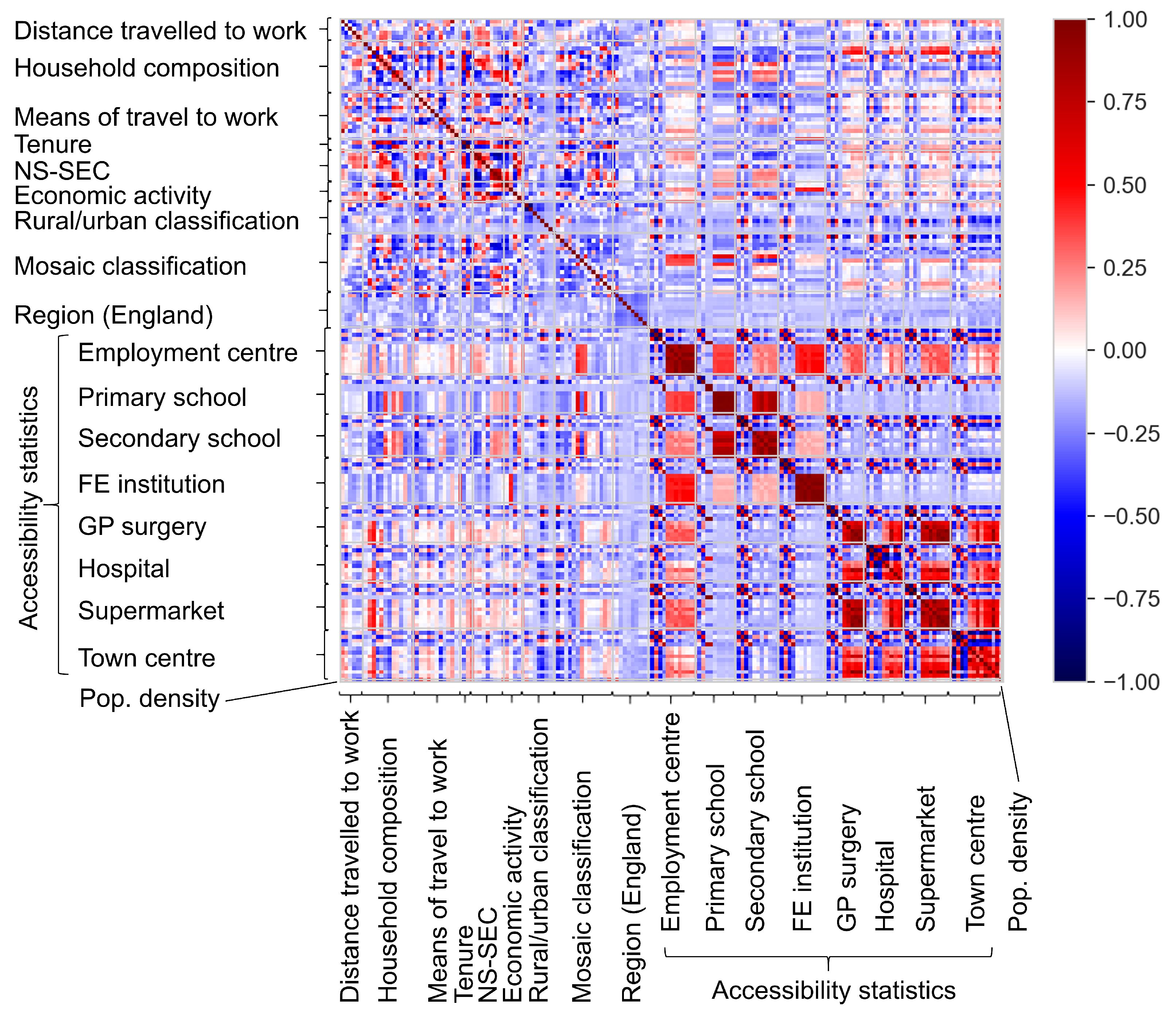
Figure 1 shows a correlation matrix between 169 variables for the England dataset to demonstrate the significant level of multicollinearity in this problem.
Figure 1, which is symmetrical about the line , shows that many of the independent variables are strongly correlated with one another. The appearance of Figure 1 resembles four distinct quadrants.
The bottom-right quadrant highlights how there is a significant correlation between the levels of accessibility to each amenity. This could be expected; for example, the number of households within a 15 min drive of a primary school would be expected to influence the number of households within a 30 min drive. There is also shown to be a correlation between access to different amenities, particularly between access to employment centres and other amenities.
The bottom-left and top-right quadrants show some localised strong correlations between the accessibility statistics and other data. This is particularly apparent between household composition and propensity to live within close access to GP surgeries, hospitals, supermarkets and town centres.
The top-left quadrant shows strong correlations between many of the datasets used in this study. In particular, tenure and NS-SEC are heavily correlated with distance and means of travel to work, economic activity.
3.3. Dependent Variable
The dependent variable in this study was the number of cars & vans per LSOA/Data Zone, taken from [39]. It is important to note that this does not distinguish between different types of car ownership (e.g., leasing or owning outright). Furthermore, the only vans included in this dataset are smaller, privately-owned vans rather than delivery vans used for business and commerce. In the rest of this paper, ‘cars’ is used synonymously with ‘cars & vans’.
4. Method
4.1. Advanced Regression Models and Artificial Intelligence
Modelling the relationship between independent and dependent data (regression) is well practised in fields including (but not limited to) medicine [52,53,54], cyber security [55], finance [56], scheduling [57,58], vehicle routing [59], data classification [60] and multi-objective optimisation [61,62]. The task of regression—the prediction of this relationship—can be performed via any one of a variety of methods, including heuristics [55,59], nature-inspired algorithms [52,56,57,60,61,62] and non-linear statistical models [53,54,58].
In this study, the potential for NNs—a non-linear statistical model—to estimate the relationship between car ownership and the independent variables in Table 1 is investigated. In selection of the regression method used, four advanced regression methods were chosen: NNs, random forest (RF), stochastic gradient descent (SGD) and support vector regression (SVR). Due to their significantly higher accuracy compared to the other three advanced regression methods and OLS regression (as shown in Table 2), NNs have been used to present results from this study. In the interest of conciseness, RF, SGD and SVR are not described in detail in this paper.
4.2. Comparison to Other Regression Techniques
RF, SGD, SVR and NN regression models were designed and optimised using grid search techniques on key hyperparameters given the same dataset to return the minimum possible mean absolute error (MAE); each model was tested with an 80%:20% training:testing split. (The hyperparameters optimised for the NNs are described in detail in Section 4.5. For the RF regression model, the number of trees and the size of trees (depth; nodes per tree) were altered. For the SGD regression model, the loss function and penalty parameters were altered. For the SVR regression model, the kernel functions, and parameters —the decision surface ‘smoothness’ and significance of each training sample respectively—were altered. More detail on hyperparameter optimisation for RF, SGD and SVR regressors can be found at [63]).
Table 2 shows a comparison of the performance (given by the MAE of prediction) of the RF, SGD, SVR and NN regression models compared to that of an OLS linear regression model (Backwards elimination was used to avoid overfitting with a cut-off p-value of 0.05) on the same dataset with the same training:testing split. In Table 2, the values in brackets are the MAE values as a percentage of the average number of cars per LSOA/DZ, or the average change in cars per LSOA/DZ. As previously stated, there were 776 cars per LSOA in England, 830 cars per LSOA in Wales and 353 cars per DZ in Scotland on average. The average change in cars per LSOA/DZ between 2001 and 2011 was a positive gain of 86 cars.
As shown, significant improvements of up to 28.8% versus the OLS baseline are realised by using the NN method presented in this paper. The improvement, in percentage terms, is shown to be lower for the prediction of change in cars than for the prediction of the number of cars.
The clear out performance of NNs versus other techniques resounds with results found in a review of machine learning studies applied to problems in the energy sector in [64].
4.3. Artificial Neural Network
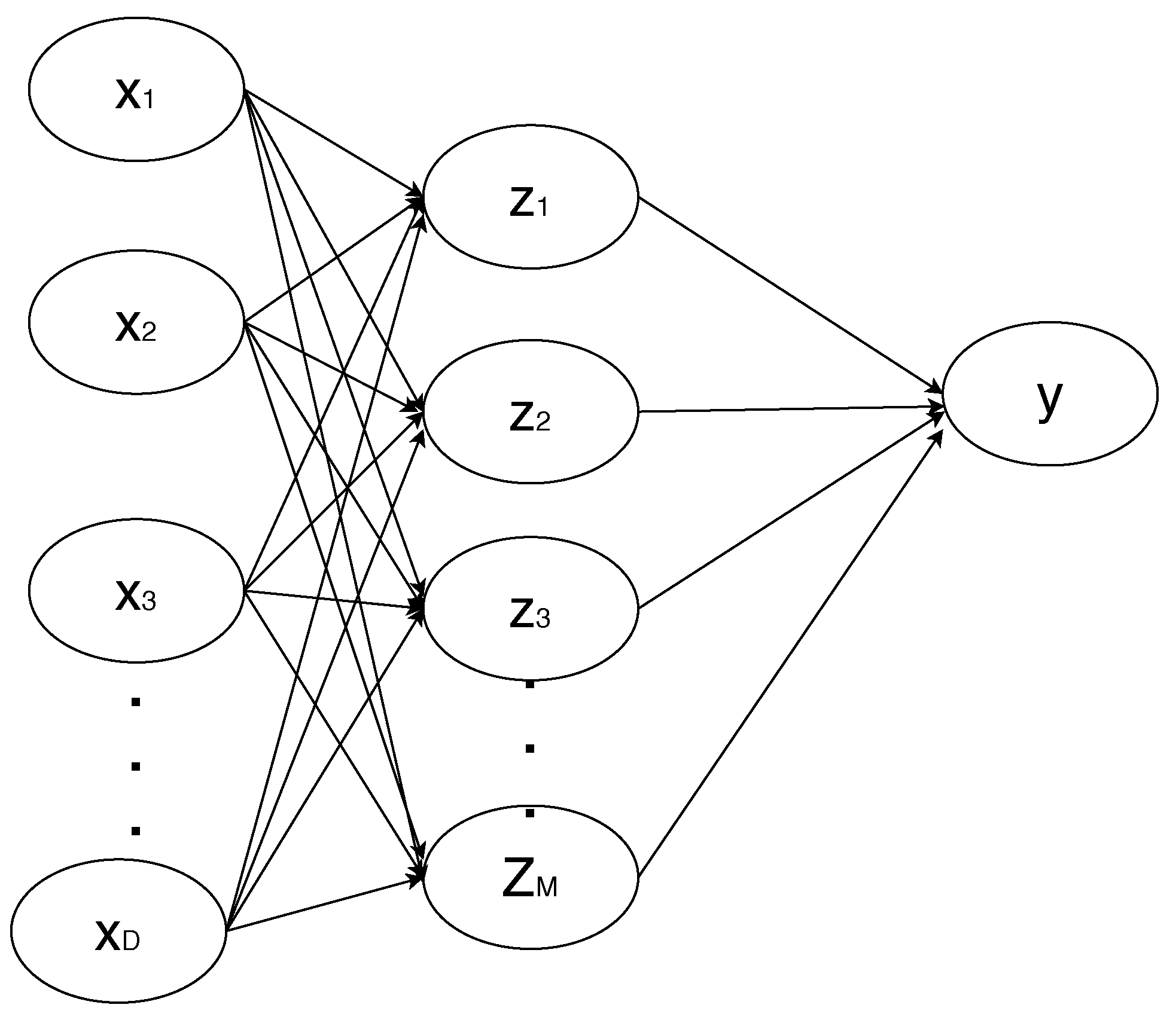
NNs are non-linear statistical models that can be used both in regression and classification tasks in machine learning applications. A linear combination of the inputs (Equation (1)) creates features, and a target variable is modelled as a function of linear combinations of the features.
Equation (1) shows the first layer of the network (as indicated by superscript 1) where , with M being the number of linear combinations. The parameters are and the parameters are biases. The quantities are known as activations. Each of them is then transformed using a differentiable, non-linear activation function h to yield the hidden units z as shown in Equation (2).
h functions vary by network design. Two of the most popular are Sigmoid and rectified linear units (ReLU) [65,66], which are both trialled in this study (Section 4.5).
A linear combination in the next layer gives output unit activations, as shown in Equation (3), where , with K being the total number of outputs. Finally, assuming that the network has one hidden layer for simplicity reasons but without loss of generality, the output unit activations are transformed through an activation function, giving a set of network outputs . The neural network is, therefore, a non-linear function, mapping the input variables to the output variables , which depend on the inputs, and a vector w that is composed by the weights and biases. A simple neural network for regression with one hidden layer can be shown in Figure 2. This configuration can be generalised by considering additional layers—‘deep’ networks are defined as those with more than one hidden layer. Each layer consists of a weighted linear combination as in Equation (3) followed by an element-wise transformation using a non-linear activation function.
While training the network, given a set of input vectors and a corresponding set of target variables, the aim is to minimise an error function . This requires an iterative optimisation process; a weight vector w which minimises the chosen error function must be found. This involves choosing some initial value for the weight vector and then moving through weight space in a succession of steps, as in Equation (4), where is the iteration step. The process by which is chosen varies by what distribution the values are selected from. In this study, normal and uniform distributions are trialled.
The choice of the vector update depends on the algorithm. Many algorithms make use of gradient information and therefore require that, after each update, the value of is evaluated at the new weight vector . (The algorithm used in this paper was the Adam optimiser [67], based on stochastic gradient descent.) The learning rate determines the step size at each iteration while moving towards a minimum of the error loss function, as shown in Equation (5).
For computational reasons, it is common practice to divide the data into smaller datasets and update the weights of the neural networks at the end of every step to fit it to the data given. The batch size is the total number of training examples present in a single batch; this is further discussed in Section 4.5.
Model parameters are internal to the neural network—for example, neuron weights w. They are estimated from the training samples and specify how to transform the input data into the desired output. On the other hand, a hyperparameter is one whose value is set before the learning process begins. Hyperparameters are not updated during the learning and are used to configure either the model (e.g., number of neurons) or the algorithm used to find the minimum error solution (e.g., the learning rate).
Hyperparameter tuning is choosing a set of optimal hyperparameters for a learning algorithm. This is carried out in this study via a grid search approach, in which a specified subset of hyperparameters is searched exhaustively to produce the best (i.e., the one that returns the lowest MSE) configuration. This is further discussed in Section 4.5.
4.4. Preprocessing—Normalisation
Before being put into the networks, the data were normalised as per a Gaussian distribution (Equation (6)).
where each is one of the set of independent variables, with corresponding mean and standard deviation .
4.5. Hyperparameter Tuning
As discussed in Section 4.3, hyperparameter tuning is undertaken to find the NN configuration that returns the smallest error of prediction. In this study, the hyperparameters tuned were the number of hidden layers, the number of neurons in each layer, the activation function used for each layer, the batch size, the learning rate and the parameter initialisation functions.
4.5.1. Network Depth and Number of Neurons per Layer
The number of neurons in the input layer was fixed by the number of independent variables. This was 169 for England, 69 for Wales and 67 for Scotland. The difference is due to the presence of the accessibility statistics for England (see Table 1) and the 6-level urban/rural classification for Scotland (compared to an 8-level classification for England & Wales).
As this is a regression problem, the number of neurons in the output layer was fixed to 1.
The number of hidden layers (i.e., not including the input and output layers) trialled was 1 to 4 inclusive. The number of neurons in the nth hidden layer was trialled exhaustively from the set (Equation (7)), where represents the set of integer multiples of 10.
4.5.2. Learning Rate, Weightings Estimator, Batch Size, Activation Function
Learning rates trialled were 0.01 and 0.001. Batch sizes trialled were 1% and 10% of the training dataset (see Section 4.5.3). ReLU and Sigmoid activation functions are trialled for all layers. Weighting estimators for all layers trialled were of normal and uniform distributions.
4.5.3. Training
The dataset was split into training, a set of data for fitting the model, validation, a set of data with which to continually evaluate the model’s performance as hyperparameter tuning was undertaken, and testing, a set of data that the model had never seen before to evaluate the performance once the hyperparameters had been fixed. The proportions of these sets were 64%, 16% and 20% respectively.
For each combination, the network was trained for up to 10,000 epochs (this was cut short if the reported MSE did not reduce substantially over 50 epochs).
The building and training of NNs in this paper was performed using the Keras library in Python [68].
4.5.4. Optimal Configurations
The sets of optimal hyperparameters out of those trialled for each regression problem are shown in Table 3.
Table 3 shows that certain hyperparameter values were consistently found to be the best performing: a learning rate of 0.001, Normal weightings estimators and ReLU activation functions were consistently better performing than their alternatives. The minimum MSE values were reported for networks with 2 hidden layers for all regression problems, though the number of neurons in each layer differed. The batch size differed depending on the input dataset. For regressions involving the England dataset (32,802 LSOAs), the optimum batch size was 1%. For the considerably smaller Wales and Scotland datasets (1909 LSOAs and 6976 DZs respectively), a 10% batch size produced a lower MSE.
5. Results and Discussion
This section presents the results of car ownership prediction in the base year (2011) and change in car ownership between 2001 and 2011 by LSOA/DZ. For background, the mean number of cars per LSOA/DZ was 776 for England, 830 for Wales and 353 for Scotland (this is lower due to the smaller number of households per Scottish DZ than English or Welsh LSOA). The average change in cars per LSOA/DZ between 2001 and 2011 was a positive gain of 86 cars.
5.1. Base Year (2011)
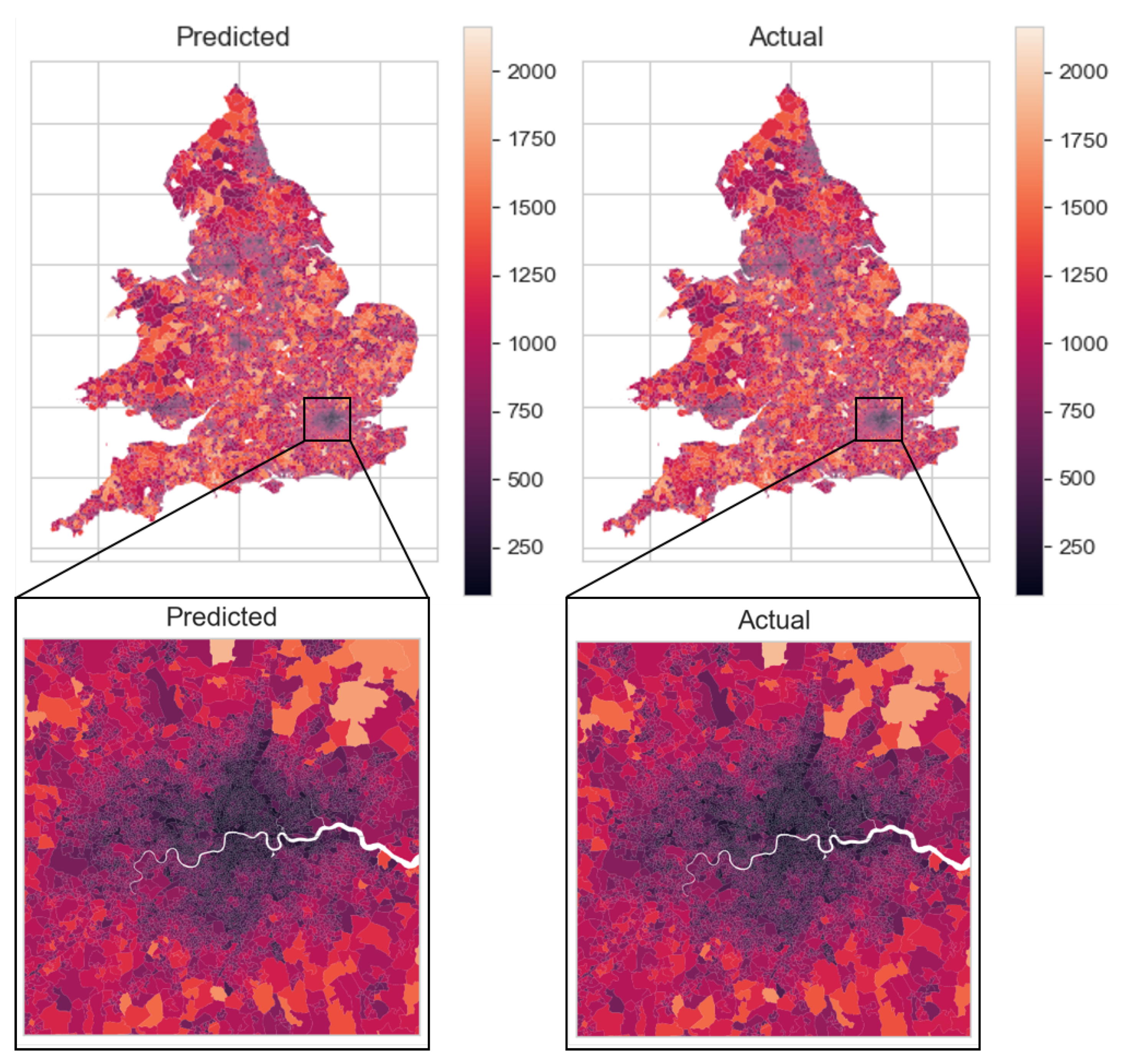
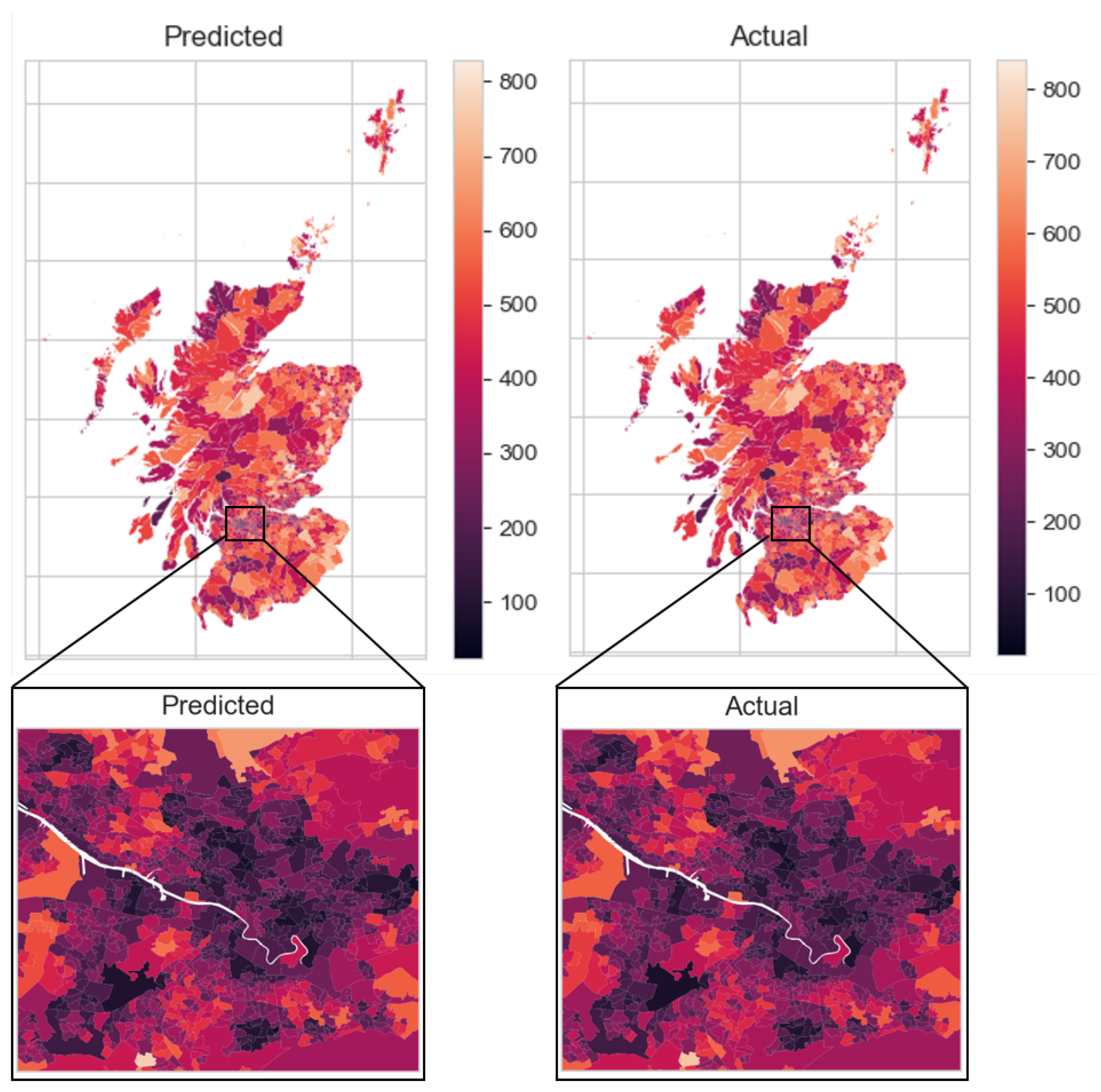
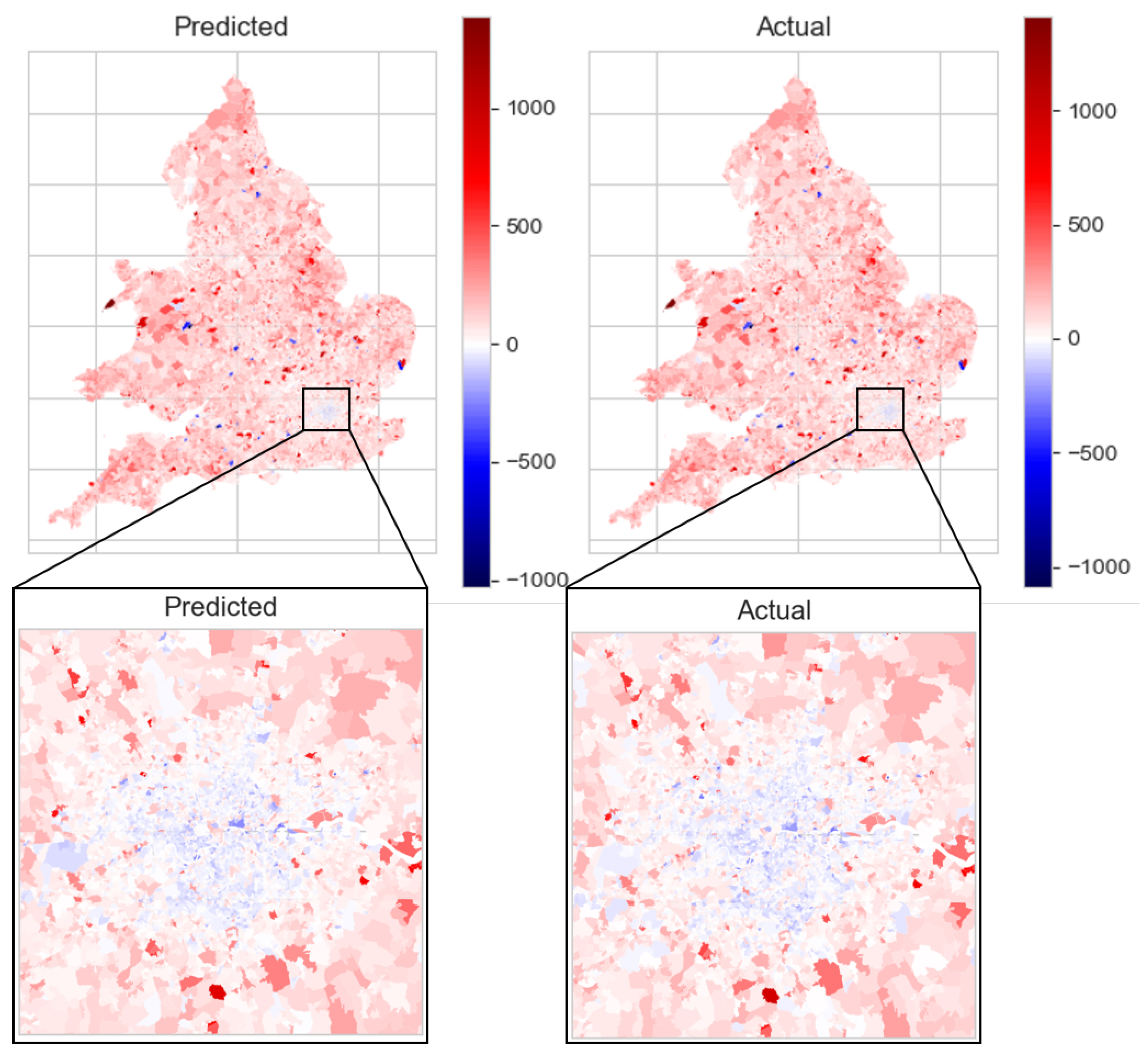
Figure 3 shows predicted and actual cars per LSOA in England & Wales; Figure 4 shows the same result per DZ for Scotland.
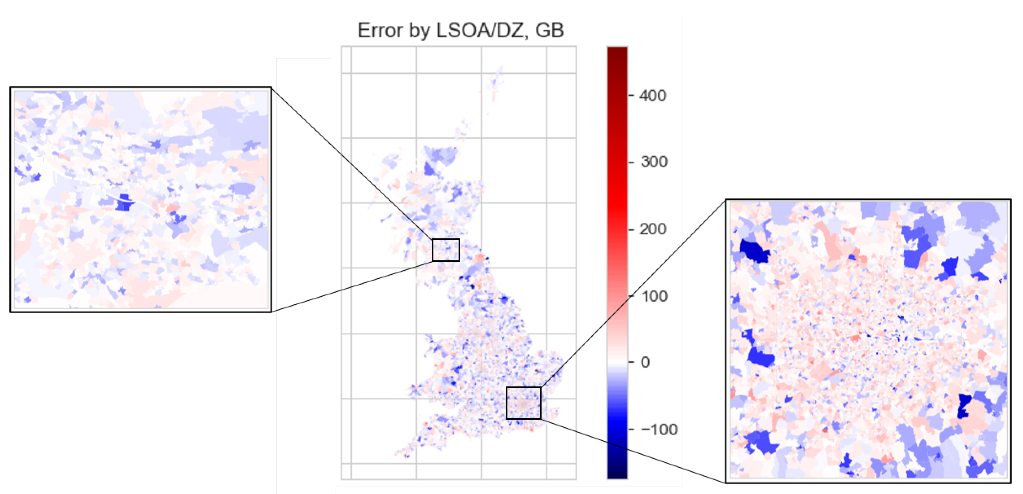
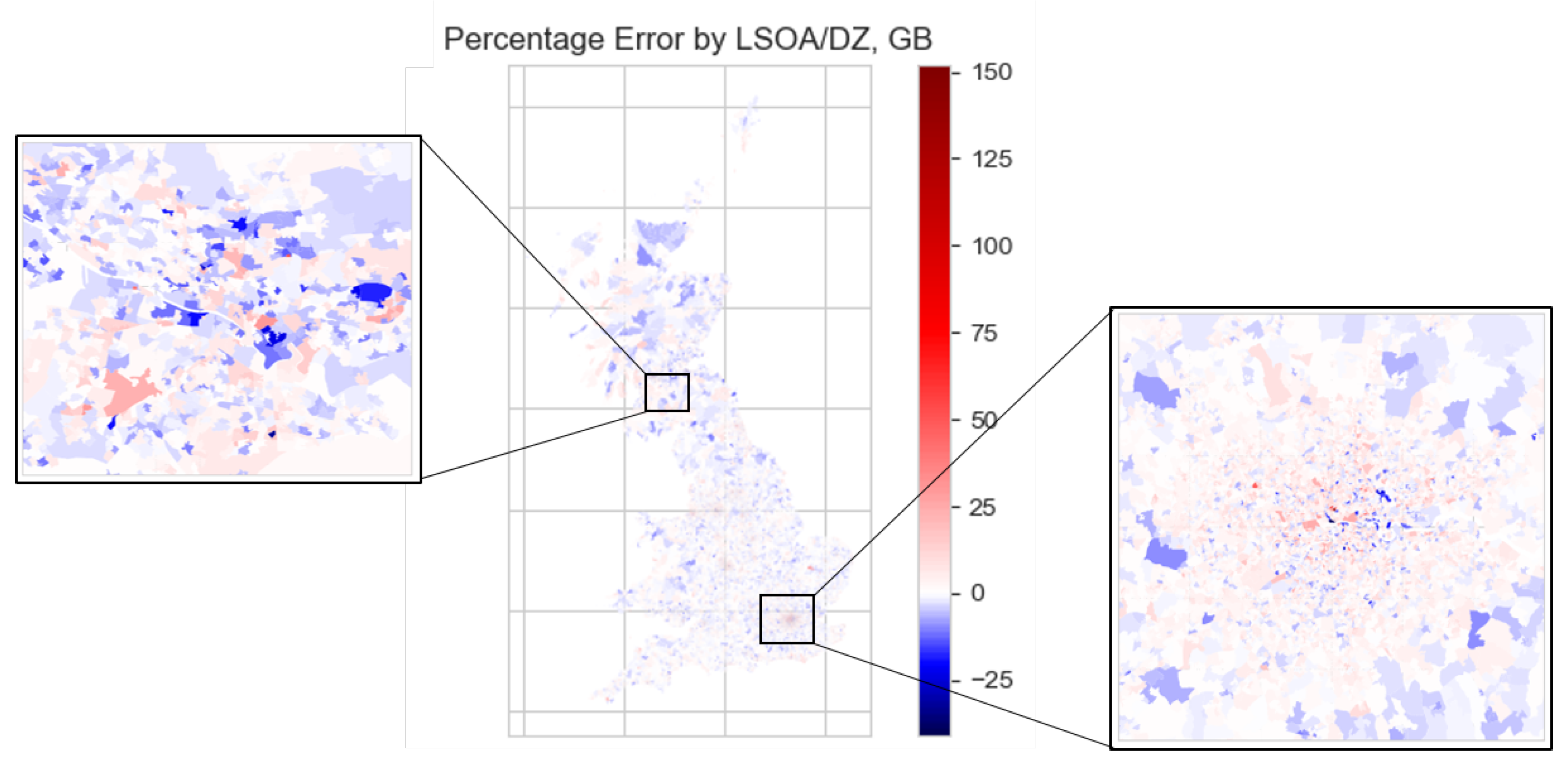
Figure 3 and Figure 4 exhibit a good prediction of the number of cars per LSOA in England & Wales and per DZ in Scotland. It is shown that generally, car ownership is higher in rural areas than urban areas (recall that LSOAs/DZs are sized on number of households)—this is a trend that has been generally observed, including in the UK [69]. While the error in prediction is difficult to make out by eye in Figure 3 and Figure 4, the error in prediction is quantified, first as a histogram and density plot in Figure 5, then displayed per LSOA/DZ for the whole of GB in Figure 6 and Figure 7.
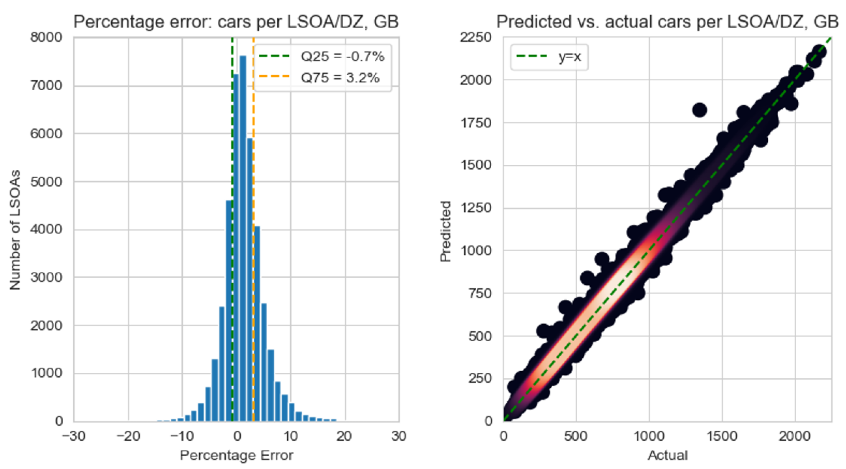
Figure 5 displays a broad goodness of fit between the actual number of cars and the predicted number of cars across GB. Half of the LSOAs/DZs are predicted within −0.7% and +3.2%, corresponding to an absolute error of −5 to +20 cars per LSOA/DZ—compared to a weighted mean of 709 cars per LSOA/DZ—across GB. The positive skew of the histogram shows that the model tends to over-predict than under-predict. This is found to be in common with the Department for Transport’s NATCOP model [21].
Figure 6 and Figure 7 show the limited correlation between prediction error and location. Though there are clearly under- and over-predictions throughout GB, it is apparent that in Greater London car ownership is generally over-predicted. This trend is also evident in other UK fleet models; for example, the aforementioned NATCOP model [21], in which it is discussed how the distinctive travel behaviours of the Greater London region lead to difficulty in predicting car ownership there. However, to this model’s credit, the errors appear to be small: whereas [21] gives an over-prediction of the total number of cars in London to be 12% (compared to over-predictions of metropolitan and non-metropolitan districts in the rest of GB to be 2% and 3% respectively), the average percentage error for this model was found to be 3.04% in London, versus a GB-wide rate of 1.35%. The mean percentage error is given for all nine English regions and the other non-English constituent countries of GB in Table 4.
5.2. Change in Car Ownership from 2001 to 2011
Figure 8 shows predicted and actual change in cars per LSOA in England & Wales.
Figure 8 shows a generally good match between the predicted and actual change in number of cars per LSOA between 2001 and 2011 in England & Wales. Extreme values in excess of +/−1000 are shown on the axis; these are due to the boundary changes in Census geography between 2001 and 2011. As discussed in Section 3.1, 2011 boundaries were used for both datasets to allow comparison; however, for a small proportion (<0.5%) of boundaries, the change in boundaries lead to drastic changes in population—and hence vehicle ownership. In general, the error appears to be small; it is difficult to see the difference between the predicted and actual plots in Figure 8. It is shown that generally, car ownership has reduced in Greater London in the period 2001–2011 and increased virtually everywhere else. This is in agreement with UK Department for Transport statistics [69].
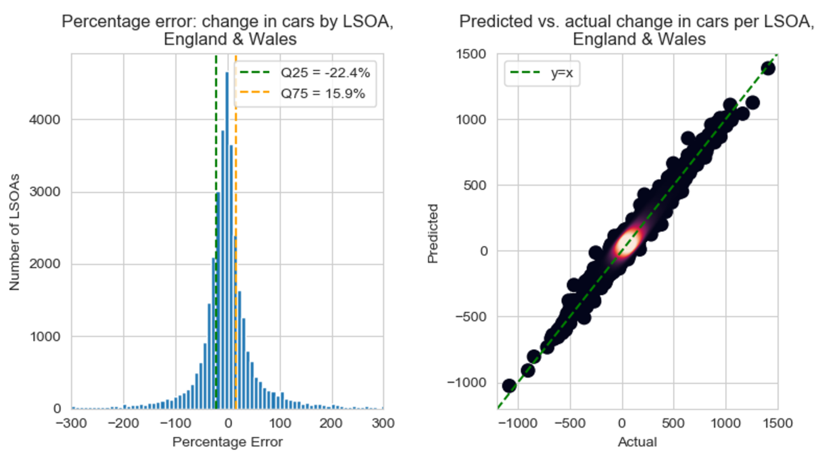
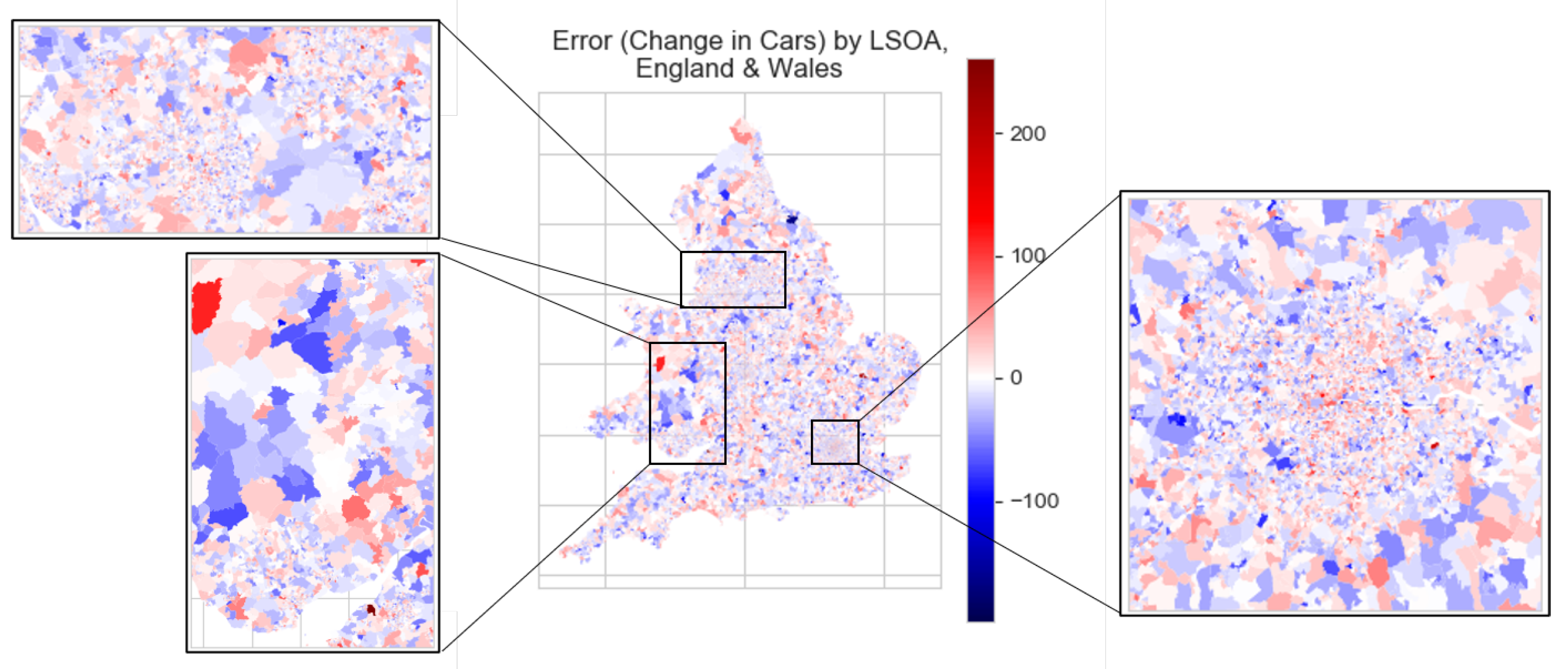
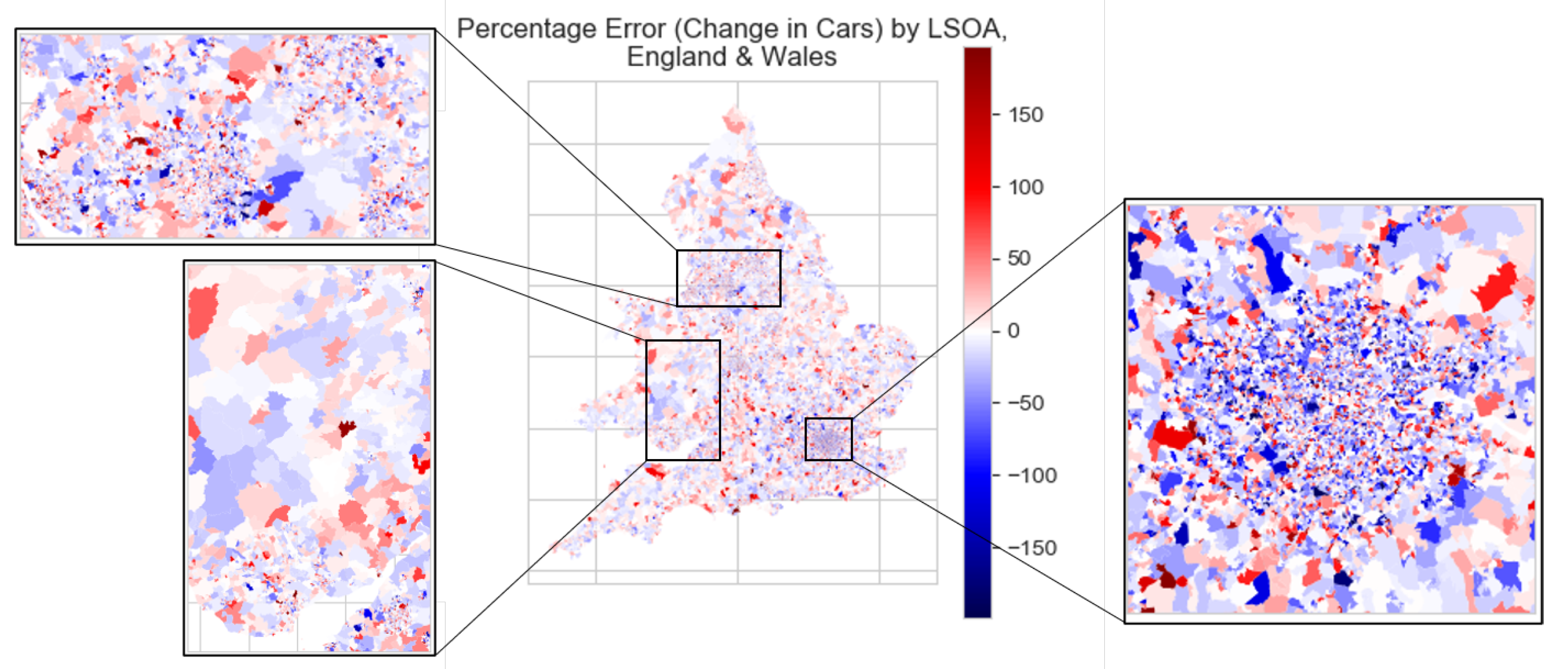
The error in prediction of the change in cars is quantified, first as a histogram and density plot in Figure 9, then displayed per LSOA for England & Wales in Figure 10 and Figure 11 (for the error in number of cars and in percentage terms respectively).
Though Figure 9 shows a steep-sided Gaussian distribution—as was the case in Figure 5—the percentage errors are notably larger: this time, 50% of the predictions are between −22.4% and 15.9% of the actual values, corresponding to an absolute error of −19 to +14 cars per LSOA (compared to, as already mentioned, an average increase in cars per LSOA/DZ between 2001 and 2011 of 86). Whereas the Gaussian distribution in Figure 5 was positively skewed, the distribution in Figure 9 is negatively skewed, meaning that the model tends to under-predict the (positive) change in cars. This is heavily impacted by the ‘special case’ presented by Greater London (see Table 5). The right-hand-side plot in Figure 9 shows the significant range of changes in cars by LSOA in 10 years. By comparison to the dashed green line (showing the line ), a generally strong prediction of change in cars is shown.
Figure 10 and Table 5 show less correlation between prediction and geographical location than was shown in Figure 6 and Figure 7. Figure 11 especially highlights the extremity of the under-predictions within Greater London (shown by the dark blue). This is reflected in Table 5, which shows the mean percentage error for the predicted change in cars (2001–2011) per LSOA for England & Wales, by English region and non-English GB constituent country (in this case, Wales). It is shown that whereas non-London English regions have a mean percentage error between −2.29% and +3.95%, Greater London’s corresponding value is −15.29%.
As detailed in Section 3, the set of predictors used for the change in car ownership is less comprehensive than the set used for base year car ownership (due to lack of data collection in 2001). This is likely to be a key reason for the greater errors in the change in car ownership model compared with the base year car ownership model.
Clearly, predicting car ownership patterns in Greater London is more difficult than doing so for the rest of GB (as previously mentioned in [21]). This may be due to the relative scarcity of off-street parking, advanced public transport networks and high-quality cycling infrastructure in the capital when compared to the rest of GB. Further work is recommended to investigate methods of improving prediction of car ownership in this region.
6. Conclusions and Future Work
This paper has presented predictions of car ownership based on demographic, socio-economic and built environment variables in a base year (2011), and over the course of 10 years (2001–2011), by using and tuning a set of deep NNs. It was shown that this method offers significant improvements in prediction accuracy (up to a 29% reduction in MAE) versus an OLS regression technique and further improvements compared to other advanced regression techniques using the same dataset, and that the model offers significant improvements in accuracy predicting car ownership in Greater London compared to the UK Department for Transport’s NATCOP model [21].
The method presented in this paper can be used to improve the accuracy of car ownership models and hence allow for enhanced modelling of the spatial distribution of car ownership. As previously mentioned, while the model does offer improvements in prediction of car ownership in London, the region still suffers worse predictions than the rest of GB. It is proposed that further work be performed to investigate methods of improving predictions within London using NN methods.
The approach demonstrated could be relevant to transport and electricity system planners. Exploring the effect of changing demographics, socio-economics and the built environment on the number of cars per LSOA is useful for transport planners as it indicates the pressure cars will put on local transport infrastructure; furthermore, by using these methods to explore credible futures for the dissipation of electric vehicles, the results could be invaluable to electricity network operators—who will be given an impression of the electrical demand they can expect at the relevant pieces of infrastructure. The method allows for scenario-based modelling of how the car ownership predicting variables may change in the future, and analysis of how this could affect car ownership. Several of the predictors used—most readily the accessibility statistics, but to a certain extent economic activity, means of travel to work, distance travelled to work and disposable household income—could be influenced by policy and planning decisions.
This paper lays the foundation for more detailed technology-aware fleet modelling, which would form a crucial part of analysis available to decision makers as the transport sector strives to meet Net Zero targets as part of Paris Agreement goals. Though this paper has focused on car ownership in GB, methods presented in this paper could readily be applied to other nations. To enhance the method’s applicability to potential disruptive patterns in the transport sector, further work is recommended to include distinction of cars by ownership type: while private owned cars dominate the UK car fleet, this may change with new business models, car clubs and other technologies—including autonomous vehicles—that may facilitate shared mobility. Of particular relevance in the future of mobility is the effect of the COVID-19 recovery on society’s willingness to use public transport [70] and the potential for the continuation of remote working [71], both of which have the potential to disrupt the future pathway of the transport-energy system.
Author Contributions
J.D.: conceptualisation, methodology, software, validation, formal analysis, writing—original draft, and writing—review and editing; S.K.: conceptualisation, methodology, writing—original draft, and writing—review and editing; C.B.: conceptualisation, methodology, writing—review and editing, supervision, and funding acquisition; M.M.: conceptualisation, methodology, and writing—review and editing; K.B.: supervision and funding acquisition. All authors have read and agreed to the published version of the manuscript.
Funding
This work was funded by the UK Energy Research Centre (UKERC) and the Centre for Research in Energy Demand Solutions (CREDS) – UK Research & Innovation grant numbers EP/S029575/1 and EP/R035288/1 respectively. The APC was funded by the same grants.
Institutional Review Board Statement
Not applicable.
Informed Consent Statement
Not applicable.
Data Availability Statement
The data used for this study are available freely online or, in some cases, to registered users of the UK Data Service. For more details, see Section 3. The code used for the regression analysis is available online https://github.com/jamesjhdixon/RegressionCarOwnership (accessed on 15 June 2021).
Conflicts of Interest
The authors declare no conflict of interest.
References
- Department for Business, Energy & Industrial Strategy. 2020 UK Greenhouse Gas Emissions, Provisional Figures; Technical Report; Department for Business, Energy & Industrial Strategy: London, UK, 2021.
- Department for Business, Energy & Industrial Strategy. UK Becomes First Major Economy to Pass Net Zero Emissions Law; Department for Business, Energy & Industrial Strategy: London, UK, 2019.
- Climate Change Committee. Net Zero: The UK’s Contribution to Stopping Global Warming; Technical Report May; Climate Change Committee: London, UK, 2019. [Google Scholar]
- Department for Transport. Decarbonising Transport: Setting the Challenge; Technical Report; Department for Transport: London, UK, 2020.
- Society of Motor Manufacturers & Traders (SMMT). Electric Vehicle and Alternatively Fuelled Vehicle Registrations: Year-to-Date; Society of Motor Manufacturers & Traders (SMMT): London, UK, 2021. [Google Scholar]
- McKerracher, C.; Izadi-Najafabadi, A.; O’Donovan, A.; Albanese, N.; Soulopolous, N.; Doherty, D.; Boers, M.; Fisher, R.; Cantor, C.; Frith, J.; et al. Electric Vehicle Outlook 2020; Technical Report; Bloomberg New Energy Finance: London, UK, 2020. [Google Scholar]
- Climate Change Committee. The Sixth Carbon Budget: The UK’s Path to Net Zero; Climate Change Committee: London, UK, 2020. [Google Scholar]
- National Grid ESO. Future Energy Scenarios; National Grid ESO: London, UK, 2020. [Google Scholar]
- Brand, C.; Götschi, T.; Dons, E.; Gerike, R.; Anaya-Boig, E.; Avila-Palencia, I.; de Nazelle, A.; Gascon, M.; Gaupp-Berghausen, M.; Iacorossi, F.; et al. The climate change mitigation impacts of active travel: Evidence from a longitudinal panel study in seven European cities. Glob. Environ. Chang. 2021, 67, 102224. [Google Scholar] [CrossRef]
- Dixon, J.; Elders, I.; Bell, K. Electric Vehicle Charging Simulations on a Real Distribution Network using Real Trial Data. In Proceedings of the IEEE Transportation Electrification Conference & Expo, Asia-Pacific, Seogwipo, Korea, 8–10 May 2019. [Google Scholar] [CrossRef] [Green Version]
- Neaimeh, M.; Wardle, R.; Jenkins, A.M.; Yi, J.; Hill, G.; Lyons, P.F.; Hübner, Y.; Blythe, P.T.; Taylor, P.C. A probabilistic approach to combining smart meter and electric vehicle charging data to investigate distribution network impacts. Appl. Energy 2015, 157, 688–698. [Google Scholar] [CrossRef] [Green Version]
- Veldman, E.; Verzijlbergh, R.A. Distribution grid impacts of smart electric vehicle charging from different perspectives. IEEE Trans. Smart Grid 2015, 6, 333–342. [Google Scholar] [CrossRef]
- Pieltain Fernández, L.; Gómez San Román, T.; Cossent, R.; Mateo Domingo, C.; Frías, P. Assessment of the impact of plug-in electric vehicles on distribution networks. IEEE Trans. Power Syst. 2011, 26, 206–213. [Google Scholar] [CrossRef]
- Xydas, E.; Marmaras, C.; Cipcigan, L.M.; Jenkins, N.; Carroll, S.; Barker, M. A data-driven approach for characterising the charging demand of electric vehicles: A UK case study. Appl. Energy 2016, 162, 763–771. [Google Scholar] [CrossRef] [Green Version]
- Dixon, J.; Bukhsh, W.; Edmunds, C.; Bell, K. Scheduling Electric Vehicle Charging to Minimise Carbon Emissions and Wind Curtailment. Renew. Energy 2020, 161, 1072–1091. [Google Scholar] [CrossRef]
- Crozier, C.; Morstyn, T.; McCulloch, M. The opportunity for smart charging to mitigate the impact of electric vehicles on transmission and distribution systems. Appl. Energy 2020, 268, 114973. [Google Scholar] [CrossRef]
- De Jong, G.; Fox, J.; Daly, A.; Pieters, M.; Smit, R. Comparison of car ownership models. Transp. Rev. 2004, 24, 379–408. [Google Scholar] [CrossRef]
- Potoglou, D.; Kanaroglou, P.S. Modelling car ownership in urban areas: A case study of Hamilton, Canada. J. Transp. Geogr. 2008, 16, 42–54. [Google Scholar] [CrossRef]
- Shay, E.; Khattak, A.J. Automobiles, trips, and neighborhood type: Comparing environmental measures. Transp. Res. Rec. 2007, 2010, 73–82. [Google Scholar] [CrossRef]
- Wang, X.; Shao, C.; Yin, C.; Zhuge, C. Exploring the influence of built environment on car ownership and use with a spatial multilevel model: A case study of Changchun, China. Int. J. Environ. Res. Public Health 2018, 15, 1868. [Google Scholar] [CrossRef] [Green Version]
- Fox, J.; Patruni, B.; Daly, A.; Lu, H. Estimation of the National Car Ownership Model for Great Britain: 2011 Base; Technical Report; The National Academies of Sciences, Engineering, and Medicine: Washington, DC, USA, 2017. [Google Scholar] [CrossRef]
- International Transport Forum. Understanding Consumer Vehicle Choice—A New Car Fleet Model for France; Technical Report; International Transport Forum: Paris, France, 2019. [Google Scholar]
- Dargay, J.M. Determinants of car ownership in rural and urban areas: A pseudo-panel analysis. Transp. Res. Part E Logist. Transp. Rev. 2002, 38, 351–366. [Google Scholar] [CrossRef]
- Chatterton, T.J.; Anable, J.; Barnes, J.; Yeboah, G. Mapping household direct energy consumption in the United Kingdom to provide a new perspective on energy justice. Energy Res. Soc. Sci. 2016, 18, 71–87. [Google Scholar] [CrossRef] [Green Version]
- Brand, C.; Goodman, A.; Rutter, H.; Song, Y.; Ogilvie, D. Associations of individual, household and environmental characteristics with carbon dioxide emissions from motorised passenger travel. Appl. Energy 2013, 104, 158–169. [Google Scholar] [CrossRef] [PubMed] [Green Version]
- Wu, N.; Zhao, S.; Zhang, Q. A study on the determinants of private car ownership in China: Findings from the panel data. Transp. Res. Part A Policy Pract. 2016, 85, 186–195. [Google Scholar] [CrossRef]
- Gough, I.; Abdallah, S.; Johnson, V. The Distribution of Total Greenhouse Gas Emissions by Households in the UK, and Some Implications for Social Policy; Technical Report; New Economics Foundation and Centre for Analysis of Social Exclusion: London, UK, 2011. [Google Scholar]
- Cairns, S.; Chatterton, T.; Anable, J.; Wilson, E.; Ball, S.; Emmerson, P.; Barnes, J. MOT data: What scope for understanding car ownership and use at a local level? In Proceedings of the 14th Annual Transport Practitioners Meeting, Nottingham, UK, 29–30 June 2016. [Google Scholar]
- Best, H.; Wolf, C.; Meuleman, B.; Loosveldt, G.; Emonds, V. Regression Analysis: Assumptions and Diagnostics; SAGE: Newcarthon-on-Tyne, UK, 2014; pp. 83–110. [Google Scholar] [CrossRef]
- Ding, C.; Cao, X. How does the built environment at residential and work locations affect car ownership? An application of cross-classified multilevel model. J. Transp. Geogr. 2019, 75, 37–45. [Google Scholar] [CrossRef]
- De Gruyter, C.; Truong, L.T.; Taylor, E.J. Can high quality public transport support reduced car parking requirements for new residential apartments? J. Transp. Geogr. 2020, 82, 102627. [Google Scholar] [CrossRef]
- Zhong, L.; Lee, B. Carless or Car Later?: Declining Car Ownership of Millennial Households in the Puget Sound Region, Washington State. Transp. Res. Rec. J. Transp. Res. Board 2017, 2664, 69–78. [Google Scholar] [CrossRef]
- Candanedo, L.M.; Feldheim, V.; Deramaix, D. Data driven prediction models of energy use of appliances in a low-energy house. Energy Build. 2017, 140, 81–97. [Google Scholar] [CrossRef]
- Kim, T.Y.; Cho, S.B. Predicting residential energy consumption using CNN-LSTM neural networks. Energy 2019, 182, 72–81. [Google Scholar] [CrossRef]
- Chen, K.; Jiang, J.; Zheng, F.; Chen, K. A novel data-driven approach for residential electricity consumption prediction based on ensemble learning. Energy 2018, 150, 49–60. [Google Scholar] [CrossRef]
- Kaewwichian, P.; Tanwanichkul, L.; Pitaksringkarn, J. Car Ownership Demand Modeling Using Machine Learning: Decision Trees and Neural Networks. Int. J. 2019, 17, 219–230. [Google Scholar] [CrossRef]
- Office for National Statistics. Lower Layer Super Output Area (LSOA) Boundaries; Office for National Statistics: London, UK, 2016.
- Scottish Government. Data Zone Boundaries 2011; Scottish Government: St Andrew’s House, UK, 2019.
- UK Data Service. Infuse—Access 2011 and 2001 UK Census Data; UK Data Service: Colchester, UK, 2011. [Google Scholar]
- Department for Transport. Accessibility Statistics; Department for Transport: London, UK, 2014.
- UK Data Service. Experian Demographic Data, 2004–2005 and 2008–2011; UK Data Service: Colchester, UK, 2011. [Google Scholar]
- Experian. Experian’s Mosaic Public Sector Citizen Classification for the United Kingdom; Technical Report; Experian: Dublin, Ireland, 2011. [Google Scholar]
- Brand, C.; Anable, J.; Morton, C. Lifestyle, efficiency and limits: Modelling transport energy and emissions using a socio-technical approach. Energy Effic. 2019, 12, 187–207. [Google Scholar] [CrossRef] [Green Version]
- Anowar, S.; Eluru, N.; Miranda-Moreno, L.F. Alternative Modeling Approaches Used for Examining Automobile Ownership: A Comprehensive Review. Transp. Rev. 2014, 34, 441–473. [Google Scholar] [CrossRef]
- Office for National Statistics. Regional Gross Disposable Household Income: Local Authorities by NUTS1 Region; Office for National Statistics: London, UK, 2020.
- Office for National Statistics. Regions (December 2017) Boundaries in England; Office for National Statistics: London, UK, 2019.
- Office for National Statistics. Rural Urban Classification (2011) of Lower Layer Super Output Areas in England and Wales; Office for National Statistics: London, UK, 2018.
- Scottish Government. Urban Rural Classification 2011–2012; Scottish Government: St Andrew’s House, UK, 2012.
- Office for National Statistics. Lower Layer Super Output Area Population Estimates; Office for National Statistics: London, UK, 2019.
- National Records of Scotland. Detailed Data Zone Tables—Mid-2011; National Records of Scotland: Edinburgh, UK, 2015.
- Office for National Statistics. Lower Layer Super Output Area (2001) to Lower Layer Super Output Area (2011) to Local Authority District (2011) Lookup in England and Wales; Office for National Statistics: London, UK, 2018.
- D’Angelo, G.; Pilla, R.; Tascini, C.; Rampone, S. A proposal for distinguishing between bacterial and viral meningitis using genetic programming and decision trees. Soft Comput. 2019, 23, 11775–11791. [Google Scholar] [CrossRef]
- Alvi, R.H.; Rahman, M.H.; Khan, A.A.S.; Rahman, R.M. Deep learning approach on tabular data to predict early-onset neonatal sepsis. J. Inf. Telecommun. 2021, 5, 226–246. [Google Scholar] [CrossRef]
- Bodenhofer, U.; Haslinger-Eisterer, B.; Minichmayer, A.; Hermanutz, G.; Meier, J. Machine learning-based risk profile classification of patients undergoing elective heart valve surgery. Eur. J. Cardio-Thorac. Surg. 2021, 1–8. [Google Scholar] [CrossRef]
- Babagoli, M.; Aghababa, M.P.; Solouk, V. Heuristic nonlinear regression strategy for detecting phishing websites. Soft Comput. 2019, 23, 4315–4327. [Google Scholar] [CrossRef]
- Sang, B. Application of genetic algorithm and BP neural network in supply chain finance under information sharing. J. Comput. Appl. Math. 2021, 384, 113170. [Google Scholar] [CrossRef]
- Dulebenets, M.A. A novel memetic algorithm with a deterministic parameter control for efficient berth scheduling at marine container terminals. Marit. Bus. Rev. 2017, 2, 302–330. [Google Scholar] [CrossRef] [Green Version]
- Brahmia, I.; Wang, J.; Xu, H.; Wang, H.; De Oliveira, L. Robust Data Predictive Control Framework for Smart Multi-Microgrid Energy Dispatch Considering Electricity Market Uncertainty. IEEE Access 2021, 9, 32390–32404. [Google Scholar] [CrossRef]
- Pasha, J.; Dulebenets, M.A.; Kavoosi, M.; Abioye, O.F.; Wang, H.; Guo, W. An Optimization Model and Solution Algorithms for the Vehicle Routing Problem with a ‘Factory-in-a-Box’. IEEE Access 2020, 8, 134743–134763. [Google Scholar] [CrossRef]
- Panda, N.; Majhi, S.K. How Effective is the Salp Swarm Algorithm in Data Classification. In Advances in Intelligent Systems and Computing; Springer: Singapore, 2020; Volume 999, pp. 579–588. [Google Scholar] [CrossRef]
- Liu, Z.Z.; Wang, Y.; Huang, P.Q. AnD: A many-objective evolutionary algorithm with angle-based selection and shift-based density estimation. Inf. Sci. 2020, 509, 400–419. [Google Scholar] [CrossRef] [Green Version]
- Zhao, H.; Zhang, C. An online-learning-based evolutionary many-objective algorithm. Inf. Sci. 2020, 509, 1–21. [Google Scholar] [CrossRef]
- Pedregosa, F.; Varoquaux, G.; Gramfort, A.; Michel, V.; Thirion, B.; Grisel, O.; Blondel, M.; Prettenhofer, P.; Weiss, R.; Dubourg, V.; et al. Scikit-learn: Machine Learning in Python. J. Mach. Learn. Res. 2011, 12, 2825–2830. [Google Scholar]
- Sharifzadeh, M.; Sikinioti-Lock, A.; Shah, N. Machine-learning methods for integrated renewable power generation: A comparative study of artificial neural networks, support vector regression, and Gaussian Process Regression. Renew. Sustain. Energy Rev. 2019, 108, 513–538. [Google Scholar] [CrossRef]
- Friedman, J.; Hastie, T.; Tibshirani, R. The Elements of Statistical Learning; Springer Series in Statistics New York; Springer: New York, NY, USA, 2001; Volume 1. [Google Scholar]
- Sibi, P.; Allwyn Jones, S.; Siddarth, P. Analysis of different activation functions using back propagation neural networks. J. Theor. Appl. Inf. Technol. 2013, 47, 1344–1348. [Google Scholar]
- Kingma, D.P.; Ba, J.L. Adam: A method for stochastic optimization. In Proceedings of the 3rd International Conference on Learning Representations, ICLR 2015—Conference Track Proceedings, San Diego, CA, USA, 7–9 May 2015; pp. 1–15. [Google Scholar]
- Chollet, F. Keras. 2015. Available online: https://github.com/fchollet/keras (accessed on 8 March 2021).
- Department for Transport. Household Car Ownership by Region and Rural-Urban Classifcation: England, 2002/03 and 2018/19 (Table NTS9902); Department for Transport: London, UK, 2020.
- Wiseman, Y. COVID-19 Along with Autonomous Vehicles will Put an End to Rail Systems in Isolated Territories. IEEE Intell. Transp. Syst. Mag. 2021. [Google Scholar] [CrossRef]
- Beck, M.J.; Hensher, D.A.; Wei, E. Slowly coming out of COVID-19 restrictions in Australia: Implications for working from home and commuting trips by car and public transport. J. Transp. Geogr. 2020, 88, 102846. [Google Scholar] [CrossRef] [PubMed]
Figure 1.
Correlation matrix showing collinearity of independent variables.

Figure 2.
Neural network diagram. The input, hidden, and output variables are represented by nodes. Arrows show the direction of information during forward propagation. Each hidden and output unit has an associated bias parameter (omitted for clarity).
Figure 2.
Neural network diagram. The input, hidden, and output variables are represented by nodes. Arrows show the direction of information during forward propagation. Each hidden and output unit has an associated bias parameter (omitted for clarity).

Figure 3.
Predicted (left) and actual (right) cars per LSOA (2011), England & Wales—detail shown of Greater London region.
Figure 3.
Predicted (left) and actual (right) cars per LSOA (2011), England & Wales—detail shown of Greater London region.

Figure 4.
Predicted (left) and actual (right) cars per DZ (2011), Scotland—detail shown of Greater Glasgow region.
Figure 4.
Predicted (left) and actual (right) cars per DZ (2011), Scotland—detail shown of Greater Glasgow region.

Figure 5.
Error of prediction of cars per LSOA/DZ shown through (left) histogram of percentage error by LSOA/DZ (2011) across GB and (right) density plot of predicted vs. actual cars per LSOA/DZ (2011) across GB.
Figure 5.
Error of prediction of cars per LSOA/DZ shown through (left) histogram of percentage error by LSOA/DZ (2011) across GB and (right) density plot of predicted vs. actual cars per LSOA/DZ (2011) across GB.

Figure 6.
Error of prediction of number of cars (2011) by LSOA/DZ across GB—detail shown of Greater London and Greater Glasgow regions.
Figure 6.
Error of prediction of number of cars (2011) by LSOA/DZ across GB—detail shown of Greater London and Greater Glasgow regions.

Figure 7.
Percentage error of prediction of number of cars (2011) by LSOA/DZ across GB—detail shown of Greater London and Greater Glasgow regions.
Figure 7.
Percentage error of prediction of number of cars (2011) by LSOA/DZ across GB—detail shown of Greater London and Greater Glasgow regions.

Figure 8.
Predicted (left) and actual (right) change in cars (2001–2011) per LSOA, England & Wales.

Figure 9.
Error of prediction of change in cars (2001–2011) shown through (left) histogram of percentage error by LSOA in England & Wales and (right) density plot of predicted vs. actual cars per LSOA in England & Wales—detail shown of Greater London region.
Figure 9.
Error of prediction of change in cars (2001–2011) shown through (left) histogram of percentage error by LSOA in England & Wales and (right) density plot of predicted vs. actual cars per LSOA in England & Wales—detail shown of Greater London region.

Figure 10.
Absolute error of prediction of change in cars (2001–2011) by LSOA across England & Wales—detail shown of Greater London, Northwest England and Mid-Wales regions.
Figure 10.
Absolute error of prediction of change in cars (2001–2011) by LSOA across England & Wales—detail shown of Greater London, Northwest England and Mid-Wales regions.

Figure 11.
Percentage error of prediction of change in cars (2001–2011) by LSOA across England & Wales—detail shown of Greater London, Northwest England and Mid-Wales regions.
Figure 11.
Percentage error of prediction of change in cars (2001–2011) by LSOA across England & Wales—detail shown of Greater London, Northwest England and Mid-Wales regions.


Table 1.
Independent variables used for regression model.
| Variable Category | Source | Region | Years |
|---|---|---|---|
| Demographic and Socio-Economic Data | |||
| Economic activity | UK Census | GB | 2001; 2011 |
| NSSec social classification | UK Census | GB | 2001; 2011 |
| Household composition | UK Census | GB | 2001; 2011 |
| Tenure | UK Census | GB | 2001; 2011 |
| Means of travel to work | UK Census | GB | 2001; 2011 |
| Distance travelled to work | UK Census | GB | 2001; 2011 |
| Accessibility Data | |||
| Bus service frequency indicator (1–100) to nearest amenity s in set of amenities | DfT | England | 2007–2013 |
| Travel time by mode t in set of modes to nearest s in | DfT | England | 2007–2013 |
| Number of users within travel time m in set of travel times (in minutes) by t in to nearest s in | DfT | England | 2007–2013 |
| Experian Mosaic Public Sector Classification Data | |||
| Number of individuals in Mosaic Public Sector groups (‘A’–‘O’) | Experian | GB | 2004–2005; 2008–2011 |
| Gross Disposable Household Income | |||
| Gross disposable household income per Local Authority | ONS | GB | 1997–2017 |
| Geographic Data | |||
| English region (9 levels; e.g., ‘North West’) | ONS | England | - |
| Urban/rural classification (England & Wales, 8 levels) | ONS | England & Wales | 2001; 2011 |
| Urban/rural classification (Scotland, 6 levels) | Scottish Government | Scotland | 2001; 2011 |
| Population density (England & Wales) | ONS | England & Wales | 2001; 2011 |
| Population density (Scotland) | Scottish Government | Scotland | 2001; 2011 |
† Used for prediction car ownership 2011; ‡ used for prediction of change in car ownership 2001–2011.
Table 2.
Comparative results for mean absolute error (MAE) and MAE as a percentage of the mean number of cars per LSOA/DZ—ordinary least squares (OLS) regression; random forest (RF); stochastic gradient descent (SGD); support vector regression (SVR); artificial neural networks (NN) with optimal hyperparameters.
| Regression | OLS | RF | SGD | SVR | NN |
|---|---|---|---|---|---|
| Cars per LSOA, England | 24.66 (3.18%) | 30.17 (3.89%) | 48.89 (6.30%) | 72.83 (9.39%) | 17.55 (2.23%) |
| Cars per LSOA, Wales | 21.06 (2.54%) | 33.62 (4.05%) | 22.39 (2.70%) | 154.21 (18.59%) | 17.03 (2.05%) |
| Cars per LSOA, Scotland | 13.27 (3.76%) | 16.71 (4.73%) | 13.43 (3.81%) | 34.07 (9.65%) | 10.38 (2.94%) |
| Change in cars per LSOA, England & Wales | 21.54 (25.08%) | 23.37 (27.21%) | 21.78 (25.36%) | 36.38 (42.36%) | 19.62 (22.85%) |
Table 3.
Optimal configurations for artificial neural networks used to predict number of cars per LSOA and change in cars per LSOA.
Table 3.
Optimal configurations for artificial neural networks used to predict number of cars per LSOA and change in cars per LSOA.
| Regression | Hidden Layers | Hidden Layer Dimensions | Weightings Estimator | Activation Function | Batch Size (% of Input Data) | Learning Rate |
|---|---|---|---|---|---|---|
| Cars per LSOA—England | 2 | [100,60] | Normal | ReLU | 1 | 0.001 |
| Cars per LSOA—Wales | 2 | [40,30] | Normal | ReLU | 10 | 0.001 |
| Cars per LSOA—Scotland | 2 | [50,50] | Normal | ReLU | 10 | 0.001 |
| Change in cars per LSOA—England & Wales | 2 | [40,40] | Normal | ReLU | 1 | 0.001 |
Table 4.
Mean percentage error for prediction in number of cars (2011), English regions, Scotland and Wales.
Table 4.
Mean percentage error for prediction in number of cars (2011), English regions, Scotland and Wales.
| Region/Country | Mean Error (%) |
|---|---|
| London | +3.05 |
| North West | +1.99 |
| Yorkshire & The Humber | +1.39 |
| North East | +1.96 |
| West Midlands | +2.22 |
| South East | +1.03 |
| East of England | +0.97 |
| East Midlands | +0.98 |
| South West | +1.37 |
| Scotland | +0.11 |
| Wales | +0.02 |
Table 5.
Mean percentage error for prediction in change in cars (2001–2011), English regions and Wales.
Table 5.
Mean percentage error for prediction in change in cars (2001–2011), English regions and Wales.
| Region/Country | Mean Error (%) |
|---|---|
| London | −15.29 |
| North West | −0.12 |
| Yorkshire & The Humber | +1.26 |
| North East | +3.95 |
| West Midlands | −1.10 |
| South East | −2.15 |
| East of England | −2.29 |
| East Midlands | +1.50 |
| South West | +2.26 |
| Wales | +5.12 |
Publisher’s Note: MDPI stays neutral with regard to jurisdictional claims in published maps and institutional affiliations. |
© 2021 by the authors. Licensee MDPI, Basel, Switzerland. This article is an open access article distributed under the terms and conditions of the Creative Commons Attribution (CC BY) license (https://creativecommons.org/licenses/by/4.0/).
Share and Cite
MDPI and ACS Style
Dixon, J.; Koukoura, S.; Brand, C.; Morgan, M.; Bell, K. Spatially Disaggregated Car Ownership Prediction Using Deep Neural Networks. Future Transp. 2021, 1, 113-133. https://doi.org/10.3390/futuretransp1010008
AMA Style
Dixon J, Koukoura S, Brand C, Morgan M, Bell K. Spatially Disaggregated Car Ownership Prediction Using Deep Neural Networks. Future Transportation. 2021; 1(1):113-133. https://doi.org/10.3390/futuretransp1010008
Chicago/Turabian StyleDixon, James, Sofia Koukoura, Christian Brand, Malcolm Morgan, and Keith Bell. 2021. "Spatially Disaggregated Car Ownership Prediction Using Deep Neural Networks" Future Transportation 1, no. 1: 113-133. https://doi.org/10.3390/futuretransp1010008