
Numerical Modelling Challenges in Rock Engineering with Special Consideration of Open Pit to Underground Mine Interaction

1
Norman B. Keevil Institute of Mining Engineering, University of British Columbia, Vancouver, BC V6T 1Z4, Canada
2
Golder WSP, 2920 Virtual Way #200, Vancouver, BC V5M 0C4, Canada
*
Author to whom correspondence should be addressed.
Geosciences 2022, 12(5), 199; https://doi.org/10.3390/geosciences12050199
Submission received: 18 February 2022
/
Revised: 29 April 2022
/
Accepted: 4 May 2022
/
Published: 6 May 2022
(This article belongs to the Collection New Advances in Geotechnical Engineering)
Abstract
:This paper raises important questions about the way we approach numerical analysis in rock engineering design. The application of advanced numerical models is essential to adequately analyze and design different geotechnical aspects of pit-to-cave transitions. We present a critical review of numerical methods centered around the hypothesis that a model is not, and cannot be, a perfect imitation of reality; therefore, numerical modelling of large-scale mining projects requires the real problem to be idealized and simplified. The discussion highlights the dichotomy of continuum vs. discontinuum modelling and the important question of whether continuum models can effectively capture dynamic continuum-to-discontinuum processes typical of cave mining. The discussion is complemented by examples of hybrid continuum-discontinuum models to analyze the important problem of transitioning from surface (open pit) mining to underground mass mining (caving). The results demonstrate the hypothesis that forward modelling should be performed in the context of a risk-based approach, with numerical models becoming investigative tools to assess risk and evaluate the impact of different unknowns, thus classifying modelling outputs in terms of expected consequences.
1. Introduction
The objective of the paper is to raise important questions about the way we approach numerical analysis in rock engineering design and its validity. Some of the concerns are well-known, and yet they often remain unnoticed or undiscussed, as if we are afraid of revealing an inconvenient truth about the role of knowns and unknowns in the numerical analysis of rock engineering problems. The discussion is complemented by applications of numerical models to analyze the important problem of transitioning from surface (open pit) mining to underground mass mining (caving), thus allowing operators to extend mine life and maintain economical production of low-grade ore bodies.
The increase in global demand for mineral resources, especially those identified in critical minerals lists for sustainable and economic success, has driven the mining industry to explore and develop ore bodies with lower grade, at depth, and/or in complex geological and geotechnical settings [1]. It has been estimated that block caving projects worldwide will contribute 36% growth to mine copper production between 2019 and 2027. A major challenge for current and future underground mass mining projects is a lack of prior experience in large-scale, deep, and hard rock environments [2]. What has been termed the ‘transition problem’ has been a topic of discussion for decades—with unique economical, technical, and operational aspects to address [3].
The application of advanced numerical models is essential to adequately analyze and design different geotechnical aspects of pit-to-cave transitions (e.g., [4,5,6,7,8,9]). This paper offers a critical review of numerical methods centered around the hypothesis that a model is not, and cannot be, a perfect imitation of reality [10]. Therefore, numerical modelling of large-scale mining projects requires the real problem to be idealized and simplified. In the authors’ opinion, this simplification process affects, albeit in separate ways, both 2D and 3D models. The discussion highlights the dichotomy of continuum vs. discontinuum modelling and the important question of whether continuum models can effectively capture dynamic continuum-to-discontinuum processes typical of cave mining. In the words of Dr. Barton [11]:
“Should we spend the necessary longer time performing discontinuum models with discrete joint sets and non-linear properties? And get more realistic designs for our slopes, mines and tunnels?”
To this point, the review is supplemented by the results of a dedicated series of hybrid finite-discrete element models (FDEM) to study the controlling factors in modelling pit-to-cave transitions, including proper consideration of the effects of major geological structures. The FDEM models are not intended as a standalone case study, rather they are an integral part of the critical review. The objective is to use the FDEM results as an example of the investigative nature of forward analysis. Furthermore, they serve to demonstrate the challenges we face when selecting input variables for our models since the non-prototypal character of rock engineering design is such that our knowledge of a given rock engineering problem is—and will always be—impacted by a condition of limited information.
2. Fundamental Questions about Numerical Analysis of Rock Engineering Problems
2.1. Are Numerical Models Capable of Predicting the Future?
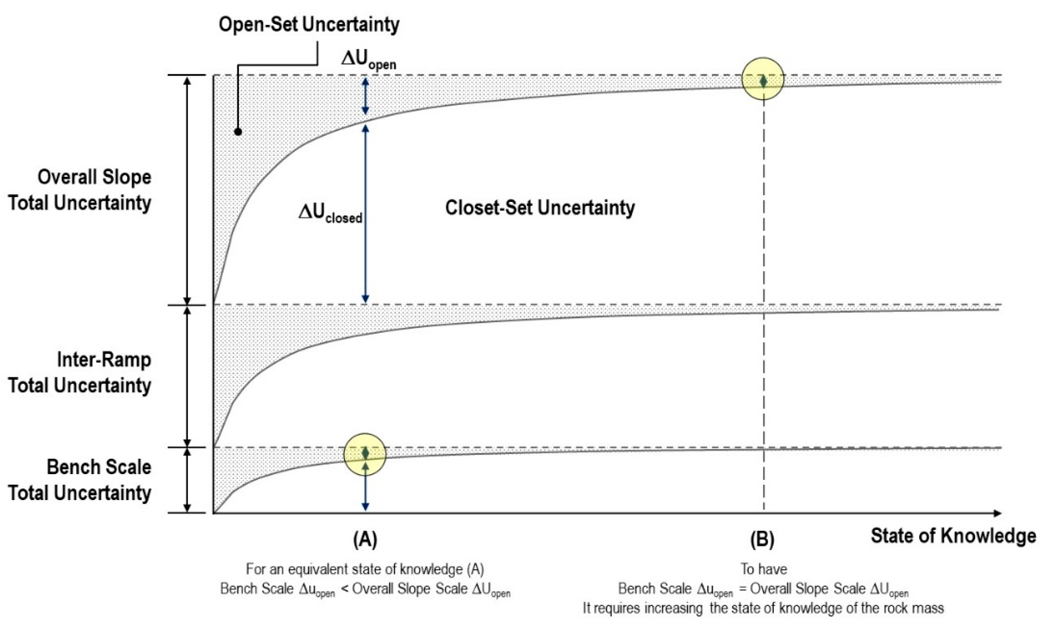
It would be impossible to begin a review of the applications of numerical models without asking the vexed question of whether numerical models can predict the future behavior of a rock mass. The word “prediction” is often used by researchers and engineers when describing the results of a series of numerical models, as if its use creates a shield of validity protecting the numerical model from critics. Predictions can be of a qualitative (e.g., type of failure mechanisms) or quantitative nature (e.g., the magnitude of deformation in a pit wall). Notwithstanding, any prediction claim, whether qualitative or quantitative, needs to face the reality of data uncertainty and data variability. The validity of any numerical analysis is strongly linked to the quality and quantity of the data used to derive the required input properties. However, in rock engineering design, collecting substantial amounts of data does not necessarily reduce uncertainty, since model and human uncertainty transcends the availability of factual data [12]. The same authors revised the concept of uncertainty as applied to rock engineering design to account for scale effects, which are ever-present in rock engineering design. Figure 1 shows the distinction between closed- and open-set uncertainty applied to pit slopes. When dealing with small scale problems (e.g., bench scale) and closed-set uncertainties, there is a point at which increasing the degree of knowledge of the rock mass would not change the design outcomes, since the impact of unknown uncertainty (unknown unknowns) is built in the design criteria by, for example, accepting a relatively large probability of failure (up to 50% for bench failure as reported in [13]). This condition is represented by Point A in Figure 1. However, pit-to-cave transitions represent large-scale rock engineering problems; as such, they belong to the domain of open-set uncertainty. Therefore, for an equivalent state of knowledge (A), we cannot exclude a priori the impact of both known and unknown uncertainty on our aggregate knowledge of the rock mass. Reducing the impact of open-set uncertainty to a level equivalent to that of bench scale problems would require a significant increase in our rock mass knowledge (Point B in Figure 1).
In their discussion about the role of cognitive biases in rock engineering, Elmo and Stead [12] borrowed terminology first introduced by [14] to distinguish between Mediocristan and Extremistan rock masses. Mediocristan rock masses are dominated by closed-set uncertainties—we can compute the probabilities of occurrence for a given event, and its impact is not significantly large. However, as projects become larger and more complex, we move into the domain of Extremistan rock masses, whereby neither empirical methods nor numerical methods can solve the problem of unknown uncertainty [12]. In the Extremistan domain, the impact of unknown uncertainty can only be accounted for by assuming artificially conservative conditions and imposing a relative larger factor of safety.
As it is not possible to completely reduce uncertainty and the potential permeation of cognitive biases in the modelling process [12], we could conclude that numerical models—from relatively simple limit equilibrium analysis to more complex 3D simulations—populate Extremistan. This argument clearly challenges the claim that numerical models could predict future conditions. The same authors argued that even in the case of a numerical model calibrated upon past conditions (backward modelling), there is no guarantee that the lessons learned from the back analysis would necessarily apply to future conditions, since there may be cases in which future conditions deviate significantly from the past ones.
The situation where future conditions may differ from past conditions is similar to that experienced during numerical models completed during the pre-feasibility and feasibility stages of a mine operation. How can the results of forward models be validated before there is an operating mine, without the data to constrain the modelling results? Should we interpret the results of numerical models for undeveloped mine sites using a confidence level approach? Table 1 (modified from [13]) lists the confidence level for several types of models (geological, structural, hydrogeological, rock mass, and geotechnical). One may argue that Table 1 fails to consider the hierarchy of the different models. For example, at the feasibility stage, a geological model has a confidence level of 65–85%—in comparison, the confidence level of the associated structural model is much smaller (45–70%). In other words, does Table 1 imply that we might know the geological characteristics of different rock units, but we do not know how they came to be placed in-situ? If that were the case, we would then expect the confidence level of the geotechnical model to be much lower since rock mass structural characteristics can play a significant role in terms of geotechnical behavior. The distinction between “rock mass” and “geotechnical” characterization is not clear; nonetheless, it would be difficult to justify a higher degree of confidence (85% vs. 80%) for geotechnical characterization when geotechnical data are not separated from rock mass data and are actually derived from it.
As discussed in [15], the rock mass characteristics of the host rock may not be well understood relative to the ore body, and drill holes purely for geotechnical/rock mass knowledge are often left until last. Logistically, this causes delays in the results of geotechnical field programs, and their inclusion in the current stage of study tends to be rushed. Accordingly, the confidence level indicated in Table 1 could likely be impacted by this process of data collection that prioritizes orebody over geotechnical knowledge. Potential areas required for infrastructure (surface or underground) development may lack adequate characterization and study to achieve the target confidence levels for the project phase.
The confidence levels in Table 1 are qualitative assessments and are, therefore, subjected to cognitive biases and subjective interpretations. Furthermore, Table 1 appears to suggest that by the time we have reached the Operation Stage, the uncertainty level of our rock mass and geotechnical knowledge may still be as high as 20%. It is doubtful that such a high level of uncertainty would be accepted in other engineering disciplines. As discussed above, this condition may be partly masked by adopting a higher factor of safety (partly and not fully due to unknown uncertainty). The authors believe that, by operating under these premises, our approach to rock engineering design would just continue to hide flaws in the data collection and data characterization process. More importantly, the tendency to accept such large levels of uncertainty could create conditions under which observed deviations from results of numerical models completed during the pre-feasibility and feasibility stages could be attributed to unexpected ground conditions, thus directing the attention away from other model shortcomings. Finally, it is interesting that the use of 3D models is introduced only at the Design and Construction stage in Table 1, highlighting that adding a three-dimensionality to models is not a condition sufficient to mitigate and reduce the uncertainty level accompanying a lack of geological, structural, hydrogeological, and geotechnical knowledge.
2.2. Continuum and Discontinuum Modelling
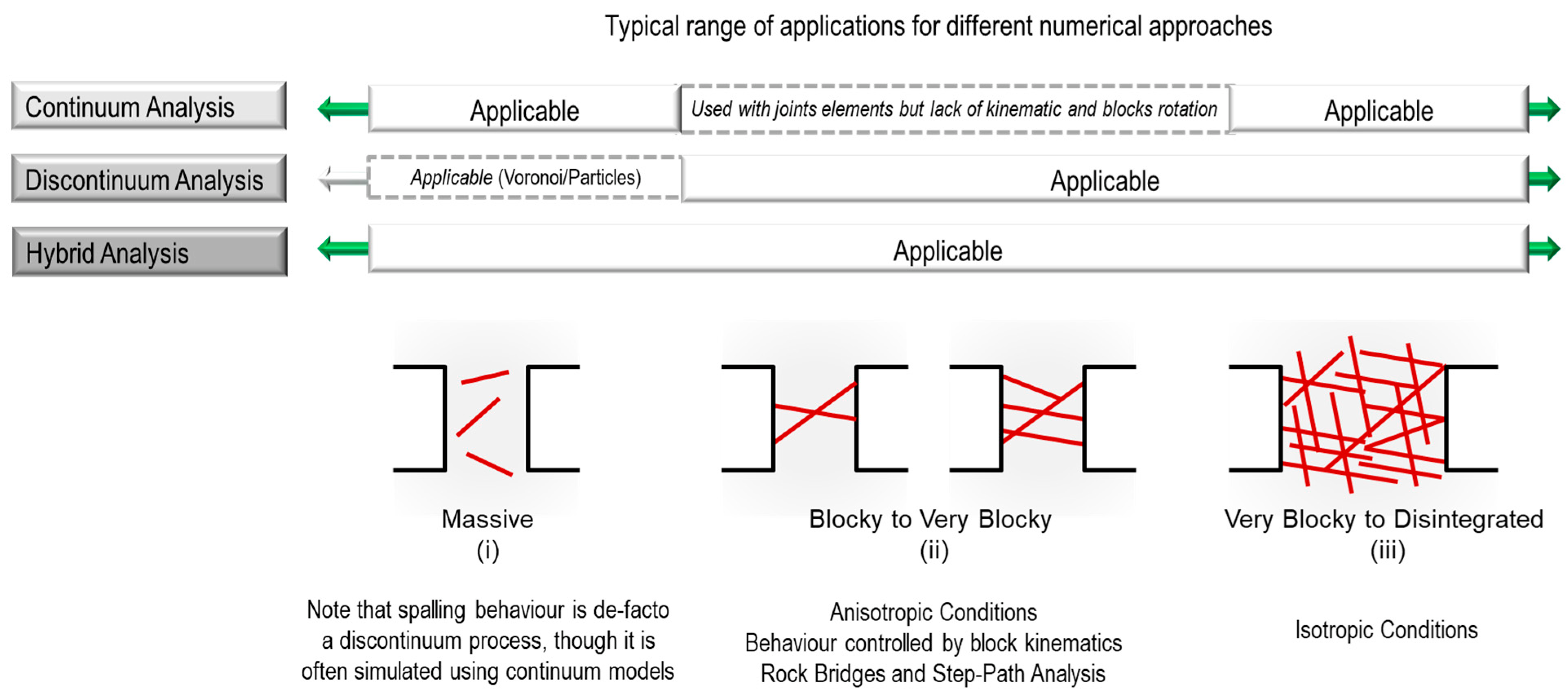
Two distinct approaches—continuum and discontinuum—are used for numerical analysis of rock mass problems; the difference between the two is the conceptualization of the problem and the deformation that can take place in the model. For instance, continuum models mainly reflect material deformations and plastic yielding, whilst discontinuum models are better at considering the kinematic components of the rock mass. The concepts of continuum and discontinuum are, however, not absolute but relative to the problem scale [16]. This is illustrated in Figure 2.
The most common types of numerical models that have found application in the solving of rock engineering problems can be grouped as follows [17]:
- Continuum methods: Boundary Element Method (BEM), Finite Element Method (FEM), and Finite Difference Method (FDM);
- Discontinuum methods: Discrete Elements Method (DEM), Discontinuous Deformation Analysis (DDA), and Discrete Fracture Network Method (DFN);
- Hybrid models: Hybrid BEM/DEM, Hybrid FEM/BEM, Hybrid FEM/DEM (FDEM), and other hybrid models.
Jing [18] and Coggan and Stead [19] provided a comprehensive review of numerical modelling techniques for rock mechanics and rock engineering. BEM models are mostly limited to elastic analysis, though non-linear and time-dependent options are available. BEM models could, in principle, be used to simulate fracturing mechanisms, though that is mostly limited to laboratory-scale simulations (e.g., [20,21]). Although both FEM and FDM models can be successfully used to simulate elastic-plastic yielding of rock masses (slopes and cave problems), they are not well-suited to explicitly simulate brittle failure (i.e., progressive damage) processes. Hajiabdolmajid [22] used FDM codes with a dedicated Mohr–Coulomb criterion with cohesion-weakening and frictional-hardening. Spreafico [23] used a FEM model incorporating polygon Voronoi joints and DFNs to simulate the brittle fracture involved in the 2014 San Leo rock slope failure in Italy.
DEM models are clearly better suited to simulate blocky media, in which deformation along joints is controlled by specified contact constitutive criteria (e.g., Mohr–Coulomb or Barton–Bandis models). When combined with Voronoi or trigon techniques, DEM models can indirectly simulate brittle failure mechanisms (e.g., [24,25,26]). The process is defined as indirect since it is not formulated upon principles of fracture mechanics and, therefore, it does not use Mode I or Mode II parameters as input. Particle flow codes (PFC; [27,28]) are an alternative discontinuum approach that has been extensively used to numerically investigate rock mass behavior. More recent developments in the application of 3D bonded particle codes include the YADE DEM code (e.g., [29,30]).
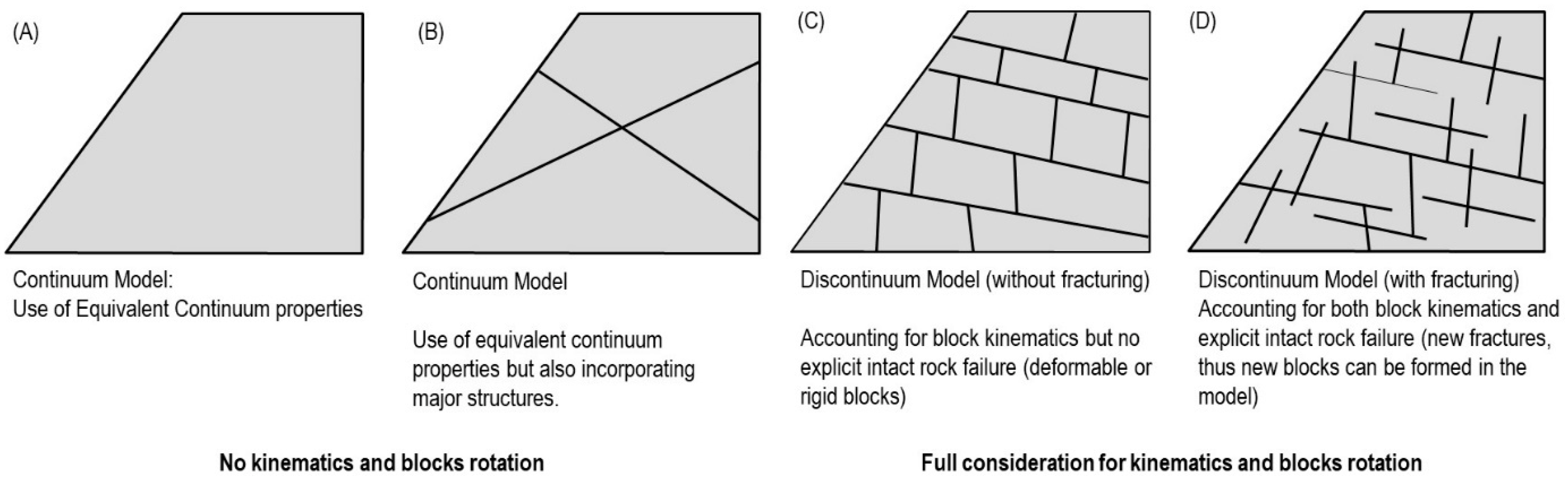
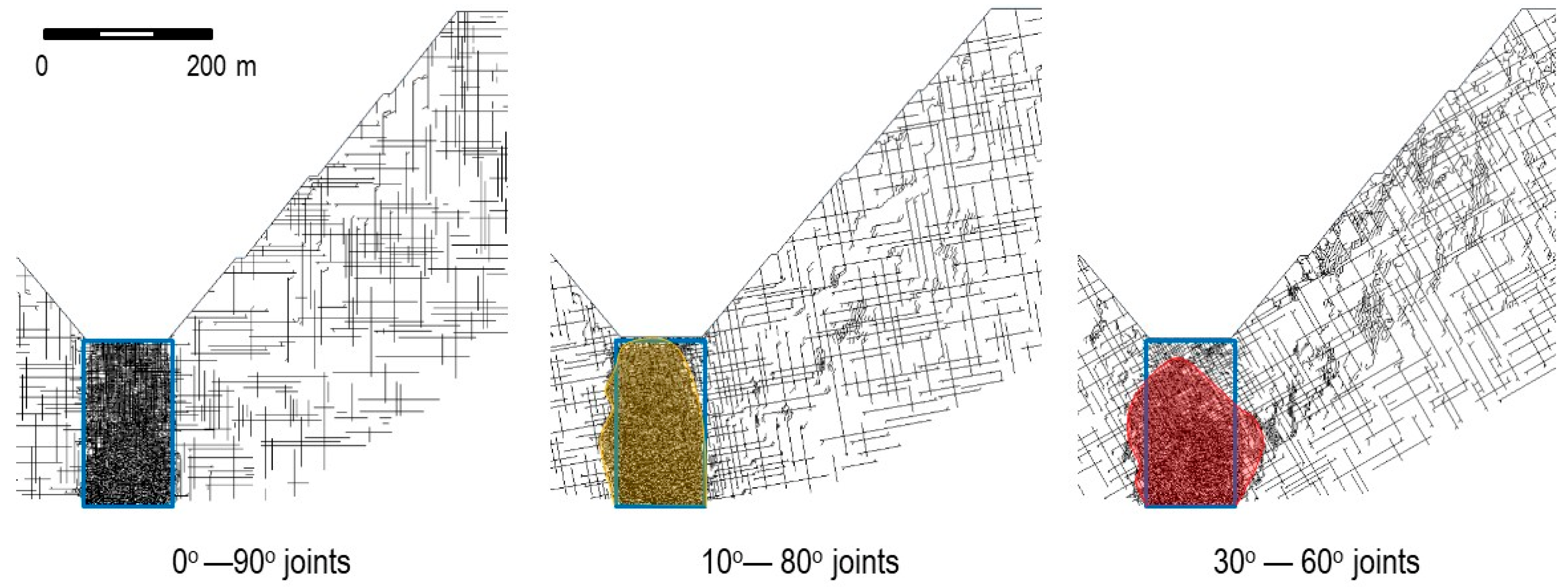
In general terms, the range of rock mass conditions where continuum modelling can be applied is limited compared to discontinuum and hybrid modelling. Nonetheless, the use of continuum models is more established due to their computational advantage (run times). We could argue that the habitual use of continuum models, in combination with equivalent continuum properties calculated using the Hoek–Brown/GSI approach creates, in the words of Kahneman [31], an “Illusion of Validity”. Rather than accepting the limitations of continuum models applied to study the behavior of fractured rock masses, we keep propagating the same justifications (faster computing times, 3D conceptualization) to justify it as an alternative to discontinuum and hybrid models. Continuum modelling trades structural complexity for geometrical simplicity (Figure 3), thus identifying the material parameters associated with specified constitutive equations for the equivalent continuum [17]. Figure 4 shows the impact of joint orientation on the stability of a slope following the caving of a 200 m high orebody, modelled using a hybrid method (modified from [5]). The results show that both cave development and subsequent slope behavior are controlled by the underlying rock mass fabric. It becomes apparent that modelling the behavior of a fractured rock slope by ignoring structural features and relying exclusively on an equivalent continuum approach without proper consideration of the impact of a “continuum homogenization process” may change the outcome in terms of the simulated rock mass behavior. The use of a ubiquitous joint approach can help circumvent this limitation (e.g., [7]).
It should be noted that any intervening simplification process adopted on the basis of reducing run times and improving mesh quality (whether considering continuum or discontinuum modelling) may also impact the results. As indicated in Figure 5, the simplification process needs to address three important questions:
- How do we reduce the impact of cognitive biases, that is, how do we decide which joints to keep and which joints to simulate implicitly?
- How do we establish the properties for the rock matrix since those cannot be the same as an equivalent continuum model?
- If using a continuum approach, will the results be impacted by a lack of consideration for progressive failure and block rotations?
This important problem was demonstrated by [32], who simulated the mechanical behavior of a synthetic rock mass in which the embedded jointed configuration was independently simplified by a senior engineer, a junior engineer, and an automated algorithm. The results showed that the adopted simplification process could have major implications for stability analysis, with the modelled strength ranging from 12 MPa (senior engineer) to 18.7 MPa (automated algorithm).
2.3. Difficult Questions and Considerations about Numerical Modelling
While it is important to consider the limitations of numerical models as predictive tools, there are multiple reasons to consider undertaking numerical modelling of rock engineering problems, including pit-to-cave transition. Generally, the use of numerical models begins during the initial design stages when there is more site-specific information allowing the project to be analyzed beyond empirical methods. Here, models can be used to understand the effects of certain geological materials and structures, the effects of geometry, and to compare different intervention and design parameters. The potential failure mechanisms attributed to each design scenario may be identified if appropriate inputs are calculated and assumed. Models are particularly useful in calculating the expected stress conditions, regions of stress concentration, and the migration of the stresses during phased pit and cave developments. Understanding stresses can lead to the interpretation of damaged areas and ways to reduce damage.
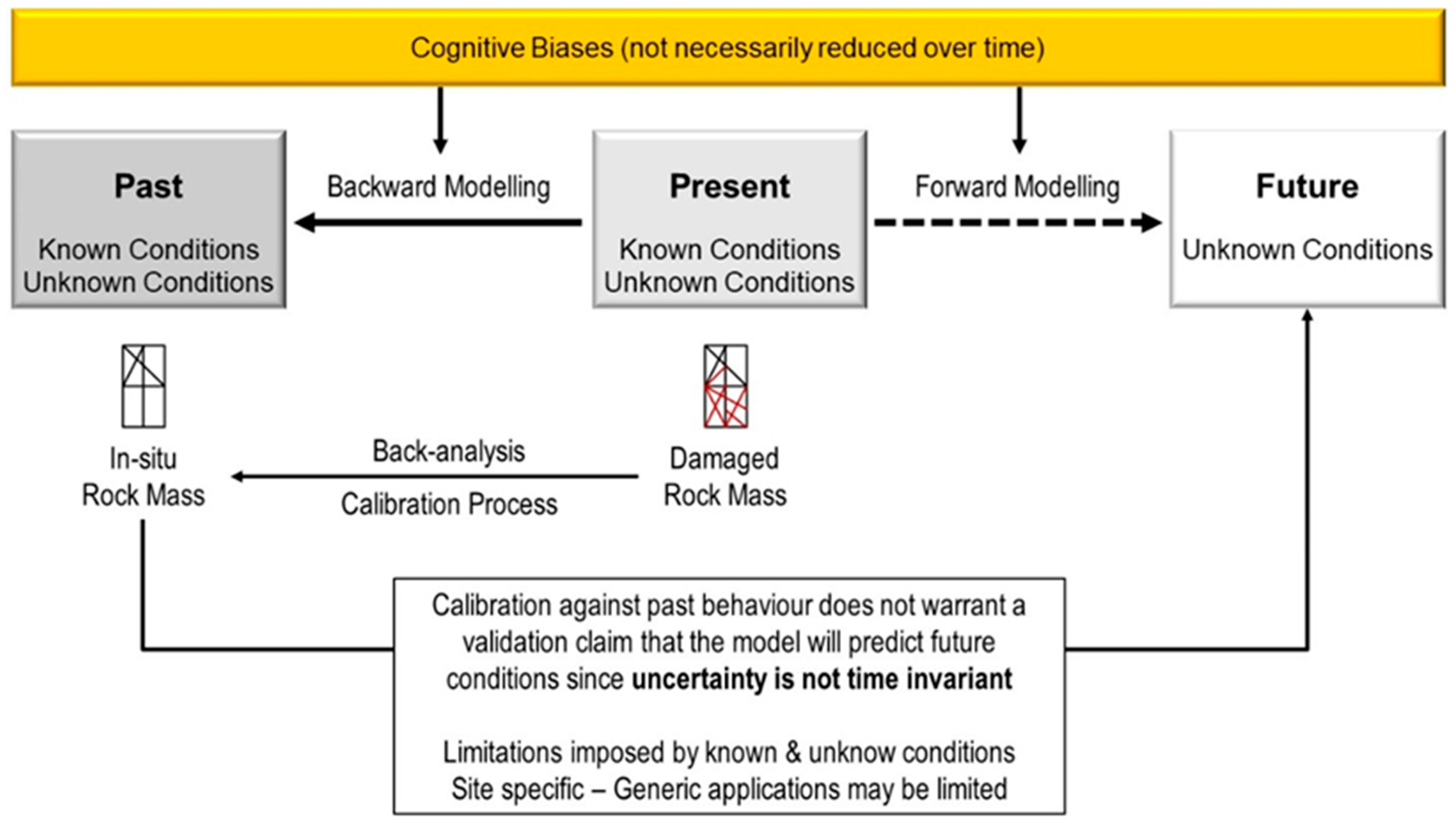
Back-analysis (backward modelling) is another common reason for pursuing numerical models. Back-analysis is generally applied to study failures that were not predicted by models in the first place. For example, in the case of the Palabora pit failure in 2004, several types of models were used in analyzing the cause of the failure and how the underlying cave caused the instability (e.g., [33,34,35,36,37]). The value of back-analysis is in knowledge creation by understanding and revealing failure mechanisms that might have been ignored or miscalculated in initial models. However, back-analysis does not solve the problem of unknown uncertainty [12], and calibrating models based on experience and understanding of other failures at the same mine site may not guarantee that a model would be able to predict the impact of future failures. In other words, back-analysis does not warrant that a validation claim based upon matching modelling results with observed field conditions could be extended to forward models and future events. As a result, if a certain modelling approach has been able to successfully back-analyze conditions at a given site, it does not justify that the same modelling parameters would be able to predict future conditions at the same site or, even more challenging, at another site where the geological conditions and failure mechanisms may be quite different (Figure 6).
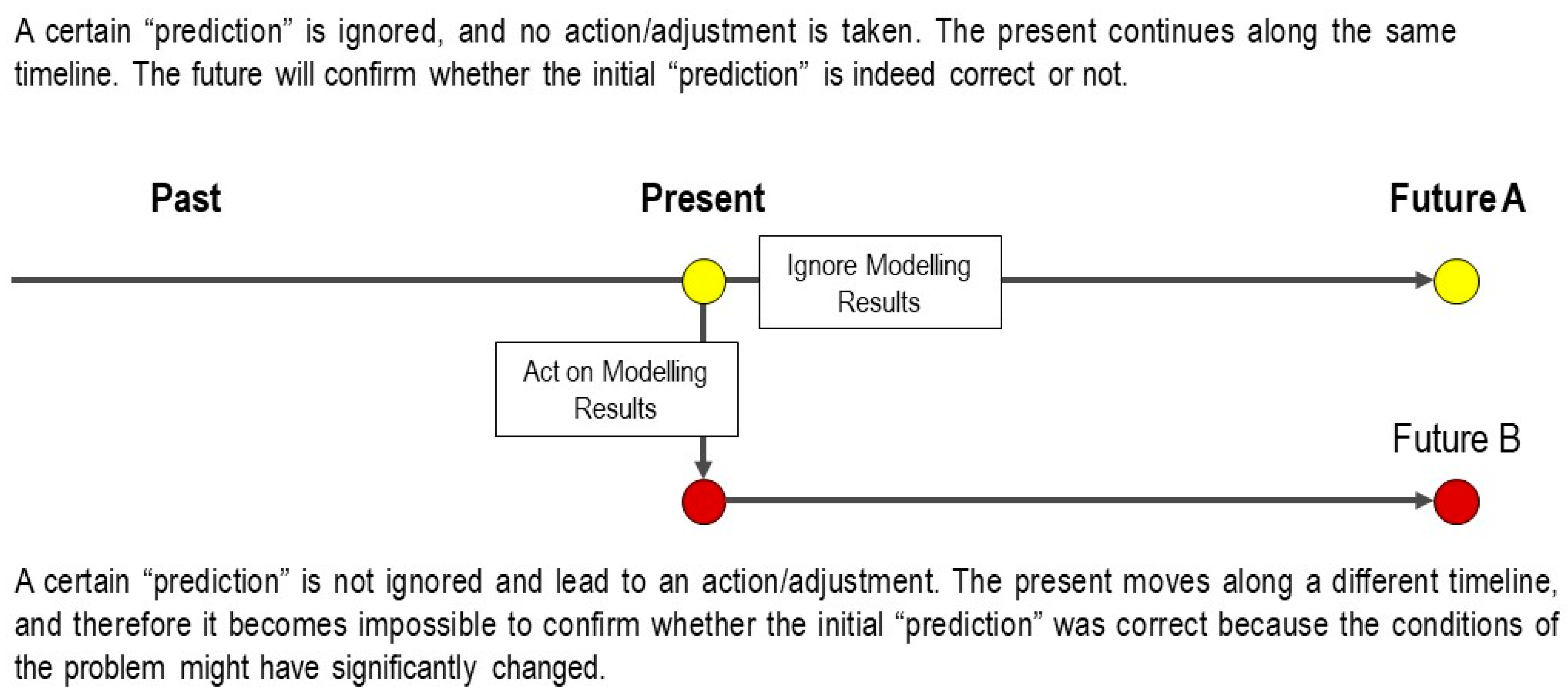
In this context, we could ask ourselves the difficult question of how many large-scale mine models completed as part of pre-feasibility and feasibility studies, when data availability is limited, have “predicted” results that agreed with observed field conditions once the mine had become operational. We argue that the objective of those forward-looking models should not be to predict rock mass behavior accurately and quantitatively but rather to frame and classify rock mass behavior under different conditions and different levels of uncertainty. This subject warrants a broader discussion on what is the role of predictions in rock engineering. How can we validate “predictions” made by a numerical model (or a machine learning algorithm, for that matter) if the “prediction” is used to change the mine design? Arguably, by changing the design (present state), we are changing future outcomes, and therefore the conditions upon which the initial “prediction” was made no longer apply (Figure 7). Decisions concerning the stability of the structure in rock are based on financial constraints, as opposed to solely geotechnical reasons, which further demonstrates the concern of the use of numerical models as investigative tools to assess risk and evaluate the impact of different unknowns.
Modelling is not intended to be a perfect solution since detailed geological conditions are seldom known. Aside from computing limitations, the numerical model works as a fit-for-purpose tool to increase the understanding of the rock mass processes involved [38]. It is up to the modeler to determine the applicability of different modelling methods for their particular analysis. Experience plays a significant role in the development and interpretation of reliable numerical models. The need for numerical models is evident when dealing with large-scale and complex rock mass systems, but their relevance in providing accurate predictions of reality must always be questioned.
2.4. Model Scale: Why “Go Big or Go Home” Is Not the Ideal Slogan for Modelling Rock Engineering Problems
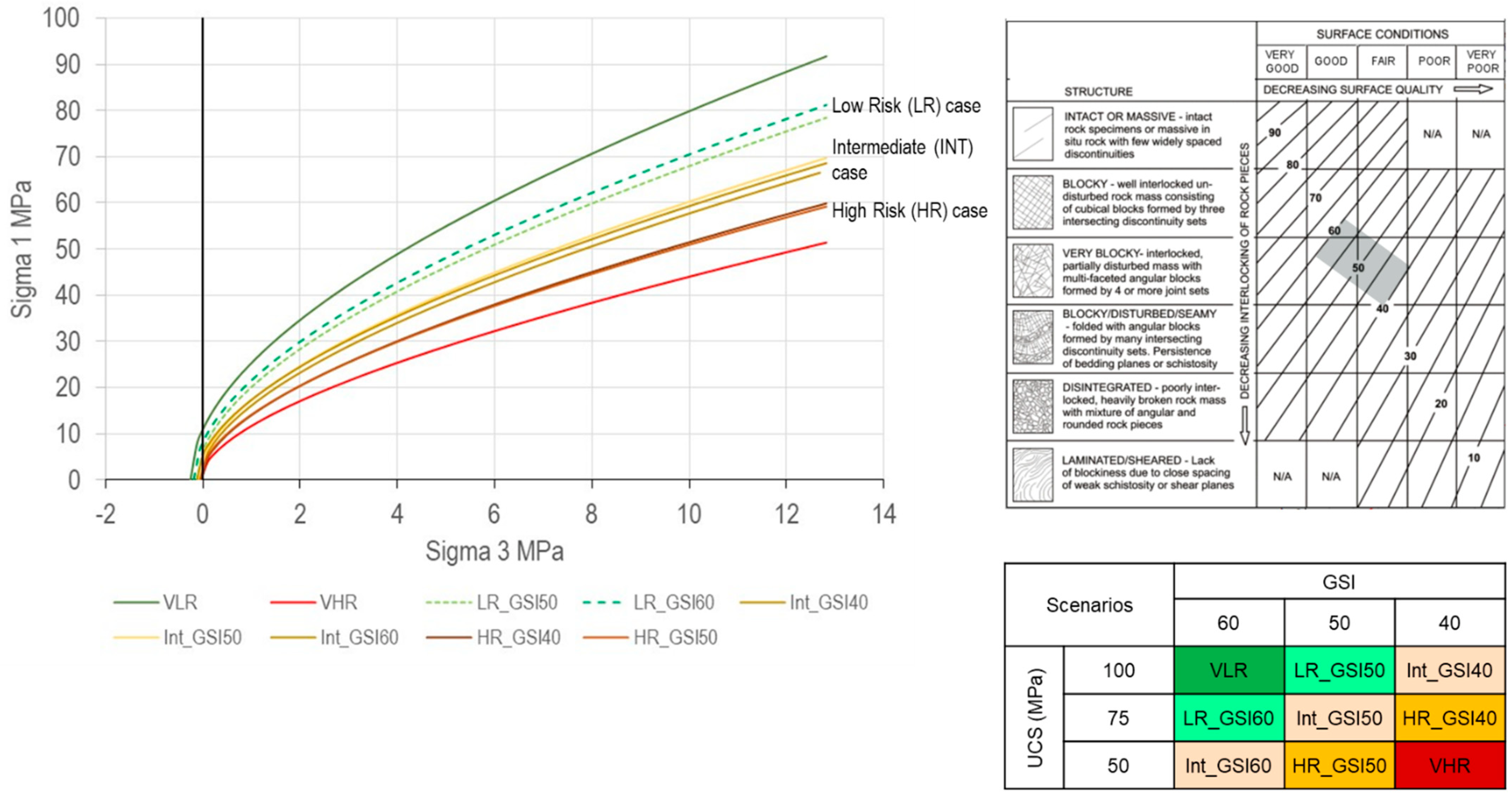
There is a tendency in the industry to discard simpler models and advertise large and complex models as the only acceptable solution to mining problems. Complex models do not necessarily provide more accurate predictions than simpler models [39]. Complexity also adds elements of uncertainty [40] since neither 2D nor 3D models alone can change the unknown and subjective nature of many geotechnical parameters. As an example, let us consider the data shown in Figure 8, representing a real field case (unnamed location) of a rock mass which is not homogeneous, neither in terms of uniaxial compressive strength nor in terms of rock mass quality (GSI). It becomes apparent that, in this particular case, it would be meaningless to attempt to model the problem by focusing on a unique set of properties. In a broader context, we would argue that the objective of forward modelling is not to provide a unique answer but rather a set of possible outcomes which can only be captured by adopting a risk-based modelling approach.
With reference to Figure 8, it is worth noting that the estimated GSI/Hoek–Brown approach yields similar failure envelopes for rather different combinations of UCS and GSI, which is the result of the underlying continuum homogenization process discussed earlier in Section 2.2.
The authors acknowledge the limitations of using a 2D approach to study 3D problems. However, the development of a 3D caving model able to incorporate fracture mechanics principles to explicitly simulate fragmentation processes at the level required to define secondary fragmentation, while also maintaining a detailed representation of the rock mass structural characteristics and simulations of preconditioning scenarios, remains one of the greatest modelling challenges in caving geomechanics. In the literature, caving models either trade the explicit consideration of fracturing and comminution processes for a 3D continuum analysis under the assumption of the rock mass being an equivalent continuum media, or they limit the explicit simulations of fracturing and comminution processes to 2D analysis. There are instances in which 3D models simulating fragmentation and cave flow mechanisms using rules-based cellular automata are coupled with 3D continuum models to study subsidence [9]. However, when applied to study pit-to-cave transition the issue remains of whether equivalent continuum slope models can capture failure processes, such as step-path failure [17], which are discontinuum in nature.
As discussed earlier, uncertainty in modelling results will increase with the scale of the considered problem, as some degree of simplification is always applied to create the model within computer limitations. With large-scale rock engineering models, it is often the underlying finite element mesh resolution that is sacrificed [41]. In brittle rock fracture mechanics processes, upscaling between laboratory testing (with fracture initiation simulated with <1 mm mesh sizes to match laboratory results) and intact rock fracture in meter-scale mesh sizes requires careful engineering judgment [41]. On this topic, we need to raise the issue of misappropriating terminology just to convey a message of greater accuracy, whether that refers to mechanisms or material parameters. The most common example in the literature is the (wrong) use of the term “microproperties”, often cited when considering the numerical simulation of rock mass behavior to give the impression that the models are capable of simulating the type of microscale failure mechanisms generally associated with the breakage of the bonds between mineral grains. That is certainly not the case for models in which the discretization size is all but micro-scale (e.g., centimeter to decimeter to meter scale). The use of the term “microproperties” is also frequently associated with DEM modelling and input properties whose magnitude is just the reflection of the adopted modelling assumptions, as this is demonstrated by the use of normal stiffness values for macro-scale discrete Voronoi contacts in the order of Tera and Peta Pascals to avoid penetration between discretized blocks.
The dependence on mesh sizes in both continuum and discontinuum modelling methods impacts the types of failure mechanisms that are able to be visualized and captured. The same applies to the selection of the required input material parameters, which would depend on the degree of simplification adopted when building the model and the choice of a continuum or discontinuum model. Concerning pit-to-cave transition models, the scale and resolution of the overall model and mesh sizes must be appropriately selected to allow simulation of both the small-scale undercut level excavations, cave propagation, and the interaction with the overlying pit and wall stability effects. Critical features should be highlighted for mesh refinement as necessary.
3. Examples of Future Modelling Challenges: Analysis of Pit-to-Cave Transition
From a modelling perspective, the problem of pit-to-cave transition presents several challenges, foremost because it involves relatively large models and simulating complex rock mass behavior by adopting either a mechanistic continuum (indirect) representation of damage processes or explicit fracturing criteria.
Currently operating block and panel cave mine operations that underly a large open pit include Palabora (South Africa), Chuquicamata (Chile), Grasberg (Indonesia), and New Afton (Canada). The Palabora pit experienced a large—caved induced—slope failure in 2004. Indeed, until recently, Palabora has served as a primary case study for transition projects under a large open pit (e.g., [33,35]). It is expected that many learnings will be leveraged for future projects, especially in regard to concurrent surface and underground operations during underground production ramp up. For example, the Chuquicamata pit (depth of approximately 1100 m) has begun transitioning to cave mining in 2018, with caving planned to be developed in three lifts, each approximately 200 m in height [42]. Another example is the Grasberg Block Cave, with column heights ranging from 250 to 500 m (dependent on pit geometry and resources) and a pit depth of 1200 m [43,44]. Red Chris (Canada) and Kerr-Sulphurets-Mitchell (KSM) (Canada) are examples of open pit and exploration projects in Canada that are planning to transition to caving. Meanwhile, several large open pit mines have deferred plans for transition to cave mining. This includes Bingham Canyon (USA), a case in which approved costs of pushbacks of the South Wall are comparable to the development of a caving operation. However, the delay in production and rectification due to the Manefay failure in April 2012 incurred additional costs [15].
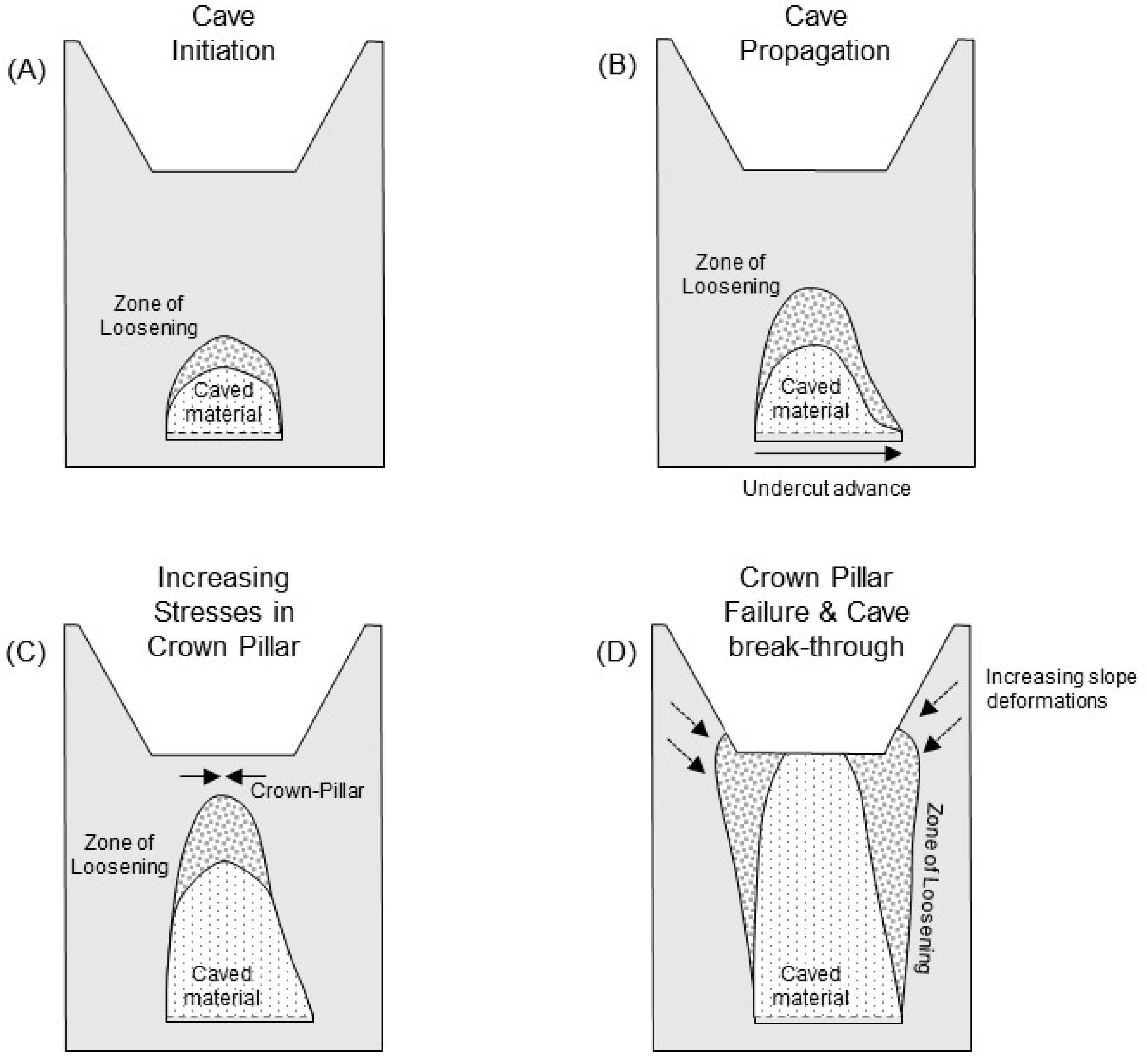
The conceptual transition process between large open pits and underground caving operations has been described as part of the International Caving Study (ICS) [45,46,47]. Figure 9 illustrates four distinct stages in a transitional operation. Note that major geological structures may impact cave development and create conditions of asymmetric cave development, which would eventually lead to pit slopes reacting differently to the induced deformations. These stages are generally visible in different numerical models simulating the caving process [8] and are illustrated in Section 3.2. Caving initiation refers to the state of the mine development where the initial undercut has been excavated. A crown pillar of decreasing thickness exists between the two mines as the cave propagates upwards, and it is this stage that determines major changes in both cave propagation and slope deformations.
The impact of the open pit on the caving operation can be significant, as hoop stresses develop during the excavation of the open pit [48]. This can result in high horizontal stresses at cave initiation at the undercut levels. While this stress state can aid in continued caving propagation, challenging ground conditions may exist during cave establishment, and preconditioning may be required for cave initiation [49]. Cavability and stresses to be expected on the production and undercut levels of the caving operation depend highly on the stress measurements and forward analysis of the post-pit stress state prior to the development of the cave. Caving schedules and advanced undercutting techniques also impact the stress field near the cave front [48].
3.1. Slope Failure and Caving Mechanisms
Unique to pit-to-cave transition projects are the effects of the caving propagation on the pit slope stability and the open pit effects on cave propagation due to an altered stress regime. Open pits are designed during feasibility studies for a particular life-of-mine timeline, and during operations, the pit slope design parameters are optimized for improved recovery to waste ratios. The optimized slope angles and bench widths associated are often not suitable for long-term infrastructure for the underground (access, vent raises, etc.) [50] and are more likely to be affected by caving propagation and crown pillar stability. Slope instabilities due to caving operations can adversely affect surface infrastructure, orebody recovery, dilution, and fines migration. In this respect, lower risk, pit-to-cave transition projects should be designed with early consideration of the highly sensitive nature of the open pit slopes to deformation underground [36].
Large-scale pit slope failures, defined as the point at which slopes have reached a displacement magnitude where it is no longer safe to operate or intended function cannot be met, include both progressive failure and rapid failure modes [13]. Focusing on inter-ramp and overall slope scale failures, the failures may include [13,51]:
- Kinematic: sliding, toppling, wedges due to joints and structures;
- Composite: a combination of stress-induced failure and sliding, rotation along pre-existing structures;
- Circular/quasi-circular/rotational: through very weak and altered rock masses and waste dumps.
As reported by Elmo and Stead [17], it is rare for rock slopes to fail without the involvement of brittle fracture, whether it is at the microscale in the fracture and removal of joint asperities or at the macroscale with the growth of persistent discontinuities to form step-paths or to allow daylighting of failure surfaces.
Caving mechanisms are based on the premise of failure of the rock mass. At shallow depth, caving is controlled by gravity loading and the degree (frequency and surface appearance) of jointing. On the other hand, the caving of massive and veined deposits at depth is governed by induced stresses (magnitude and orientation). The development of the undercut drifts causes a decrease in vertical stress and an increase in horizontal stress, with the difference magnitude determining whether sufficient rock mass yielding will result in cave initiation. Removal of the caved material (production) creates continued caving propagation, provided the differences in horizontal and vertical stress remain high (stress-driven caving at depth) or whether the tension due to gravity is sufficient to cause the collapse of the jointed rock mass (shallow deposits). Note that in the literature, the latter mechanism is often referred to as “gravity caving” to highlight the role of gravity loading in determining rock mass failure. Cave propagation behavior has been detailed by [52,53], while cave propagation under an open pit has been summarized by [5,8,47].
3.2. Hybrid FDEM Examples
The finite-discrete element method (FDEM) can efficiently analyze various aspects of cave mechanics, including cave initiation, cave propagation, draw sequence, and cave rates [4,5]. The numerical platform used in this paper is the proprietary FDEM code ELFEN [54]. Despite the approach offering a full 3D dimensional capability, this paper makes use of its 2D version to fulfill the requirement of performing a preliminary sensitivity analysis of key aspects of cave mechanics by running multiple fracturing (discrete) models at a fraction of the computational cost of a single 3D continuum model. Earlier examples of cave modelling using the same FDEM platform are presented in [5,6,36,55]. Details of the numerical formulation of the FDEM approach used in this paper are given by [38,55,56].
3.2.1. Model Setup
A series of conceptual FDEM models were run to investigate and illustrate the differences in outcomes depending on pit-to-cave transition modelling assumptions. In particular, the inclusion of major structures and discrete fabric structures, the scale of fracturing zone, and draw sequence. Table 2 provides a summary of the model scenarios presented in this paper.
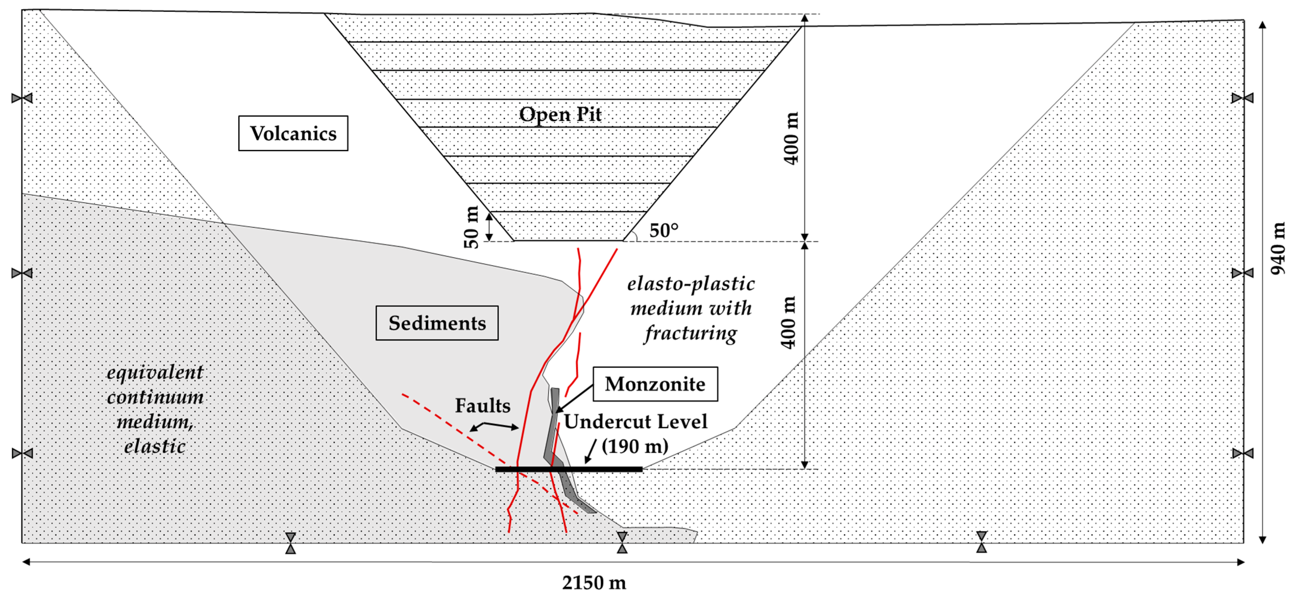
The 2D FDEM model geometry and material inputs have been modified from studies completed for an undisclosed caving mine. The primary modified model geometry, as presented in Figure 10, comprises a caving operation that is 400 m below a 400 m deep open pit with an overall slope angle of 50°. The caving undercut level is 190 m in width with an initial excavation height of 1 m. The entirety of the model measures 2150 × 940 m, subdivided into elastic and elastoplastic regions with fracturing. The non-fracturing, elastic region is required to minimize boundary effects and is modelled with a lower mesh resolution. The open pit is modelled elastically and excavated in 8 × 50 m stages. Mesh resolution varies at 1 m within the undercut level, 2 m above the undercut up to the pit bottom, and increases to 40 m near the model boundaries. Model geometry variations described in Table 2 are illustrated in Figure 11.
3.2.2. Material Parameters
Material inputs used in the FDEM models are summarized in Table 3. Specific properties derived from laboratory testing were adopted from the same undisclosed cave mine as the geometry. Rock mass properties for the coupled DFN models were assumed the same as for the equivalent continuum approach due to the scale of the discontinuities. The constitutive criterion modelled in ELFEN is based on Mohr–Coulomb with Rankine tensile cut-off. The instantaneous apparent cohesion and friction values were determined with the Hoek–Brown failure criterion, using a σ3max corresponding to 700 m overburden due to the location of the undercut level.
The strength parameters assigned to the discontinuities are defined according to a linear Mohr–Coulomb criterion, and estimates of shear and normal stiffness were based on conclusions identified by [16] and recommended relationships presented in the ELFEN user manual [54]. The caving processes modelled with FDEM are not the result of changing material properties, as they are with fully continuum models. As such, the kinematic controls are fully accounted for. The cohesion-loss, friction-hardening behavior, which is typical of brittle failure, occurs due to the explicit fracturing of the initial continuum model in ELFEN.
3.2.3. Simulation of Pit Excavation, Undercut Initiation, and Production
FDEM models are computed using incremental numerical time steps. Model time is described in seconds, and stages are defined to initiate and terminate at specific times or a specific number of time steps. The time step control settings and the stages used in the ELFEN models, defined in model seconds, are summarized in Table 4.
The open pit excavation was simulated with eight stages, with equilibrium periods defined before and after pit excavation. The undercut level was excavated in a series of five equivalent areas, with advancement from right-to-left, left-to-right, or center-out, depending on the model scenario. Symmetric draw (center-out) used three stages, while right- or left-start excavation used five stages. Excavation relaxation was completed over two seconds for each pit level and undercut level excavation.
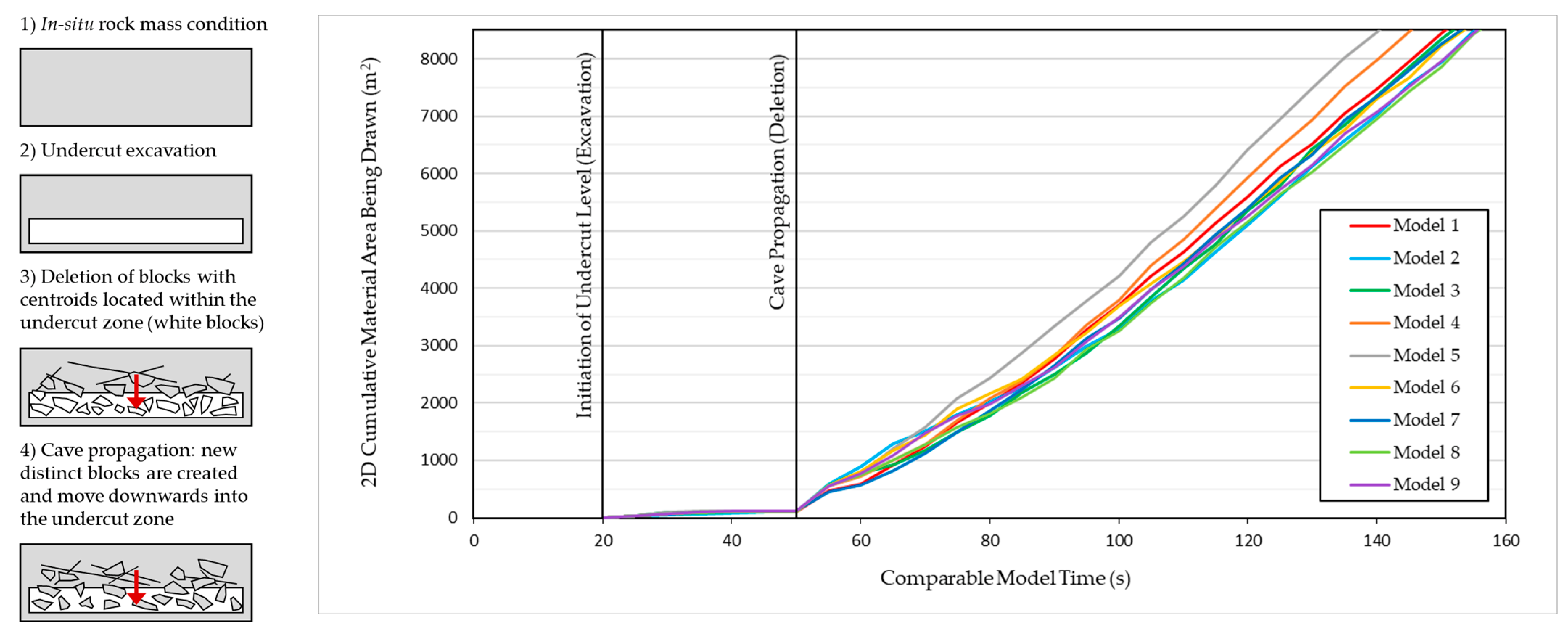
Cave propagation is caused by the removal of fractured material on the production levels. Simulating this process in FDEM models requires a series of deletion algorithms, which remove mesh elements whose centroids enter a specified region within the undercut level. The iterative deletion process, defined by specific numerical time values, was adapted from a calibrated mine production schedule of the undisclosed mine. Deletion times ranged from every 2–3 model seconds, varying between undercut level areas and the caving stage. The conceptual method of deletion for cave propagation is illustrated in Figure 12, along with the production volume (described as 2D area) for each model at comparable stages. Elmo et al. [6] describe the calibration process for the deletion algorithm to produce equivalent results in 2D compared to 3D production targets. For back-analysis models, the draw sequence and timing are calibrated to production volumes. This approach requires little user intervention, as the modeler is controlling only the deletion timing to attempt to match production, not the fracturing within the model or forcing production to occur. In this case, we adapted a previously calibrated draw sequence and timing to maintain a realistic draw, but with conceptual forward modelling and various scenarios, these models now differ from the calibrated versions and are no longer calibrated themselves.
3.2.4. Results
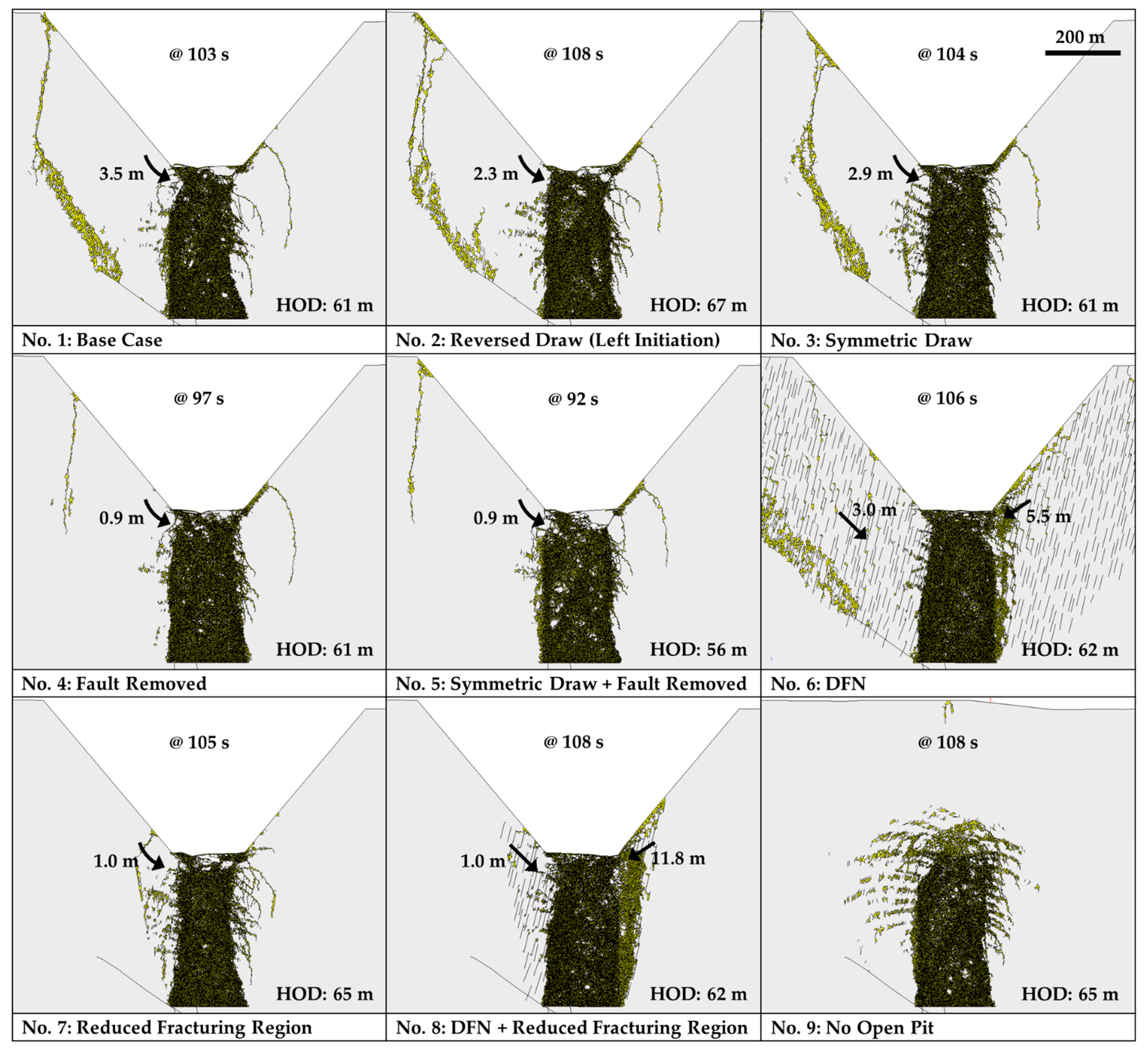
These conceptual FDEM models were created to illustrate the variability in model results based on different modelling strategies—whether simplification assumptions, trade-off decisions between scale and run-time, or lack of data defining controlling features. Nine models are presented in Figure 13, with fractured elements highlighted in yellow. Due to the variation in model timing, comparable models were selected at a specific 2D production value. In all pit models, slope failure and mobilization occurred due to caving-induced unloading. The magnitude of movement varies greatly between models with and without the fault extending left of the undercut level (No. 1 vs. No. 4, 5), those with and without a defined fracture network (No. 1 vs. No. 6, 8), and those with a differing scale of fracturing regions (No. 1 vs. No. 7, 8).
Models No. 1–3 compare draw strategy and undercut level initiation, and these results indicate that the differences are minimal in comparison to the effects of modelling scale assumptions and geological impacts. It should be noted that despite the different draw strategies tested (No. 1–3, 5), the maximum height of draw (HOD) occurs above the undercut level (UCL) areas 3–5 (right side) of all models except No. 5, where the combination of a symmetric draw strategy and the removal of the left fault created the conditions possible for a true near-symmetric draw.
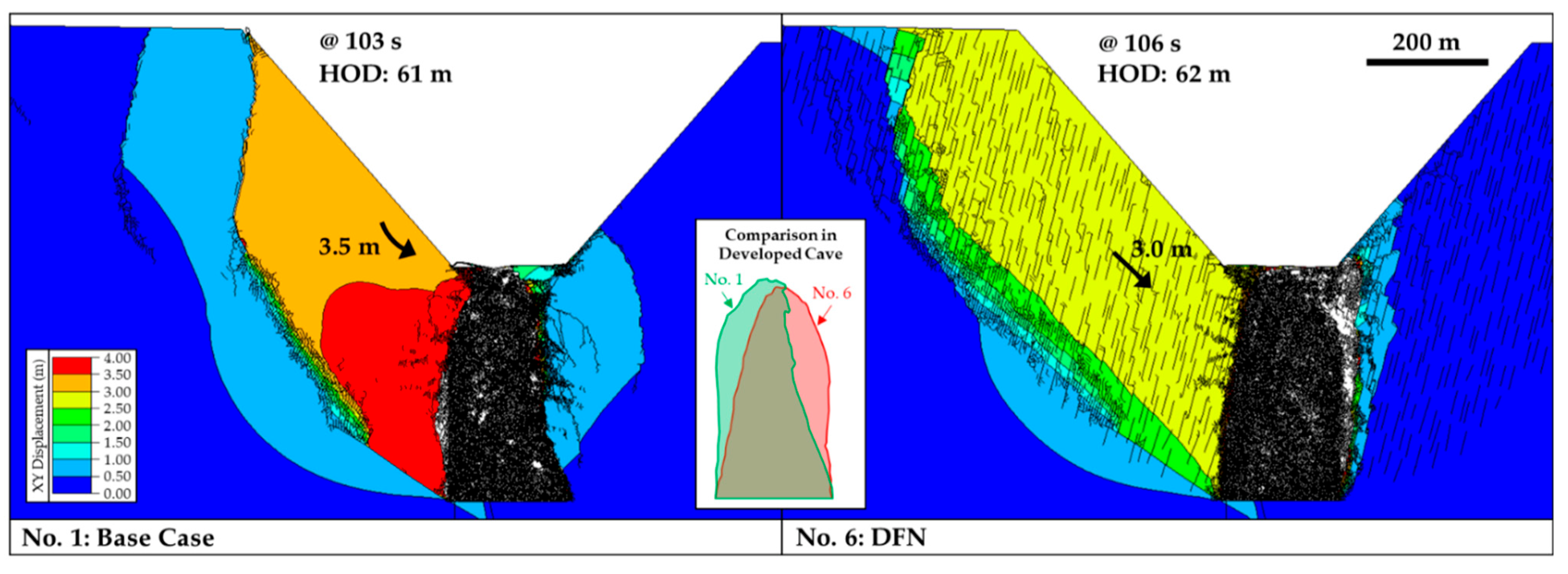
Models defined as elastoplastic with fracturing only (i.e., no DFN) developed large unrealistic tension cracks on the surface and in the pit walls (No. 1–5, No. 9). This was expected and is not an uncommon result when simulating caving mechanisms using either discontinuum or continuum models in which there is no pre-defined fracture network to release the strain associated with caving-induced deformation. The impact of the addition of the DFN is explored in greater detail in Figure 14, Figure 15 and Figure 16. Detailed comments on the results of all models are summarized in Table 5.
4. Discussion and Conclusions
Numerical analysis is not immune to the inductive nature of rock engineering design, defined by the uncertainty surrounding geological data, model parameters, human factors, and by the variability and qualitative nature of geological data. This paper helps raise important questions and concerns that all modelers should be aware of and recognize in their practice. These concerns become even more apparent when considering the difficulty of validating forward models and the incomprehensible quest to simplify and homogenize rock masses as if rock mass quality were indeed a continuum physical property.
In the authors’ opinion, notwithstanding the nature and scale of the modelling approach, forward modelling should be performed in the context of a risk-based approach, therefore classifying modelling outputs in terms of expected consequences. To this point, we have presented the results of a conceptual (i.e., 2D) analysis of transitioning from surface (open pit) mining to underground mass mining. Key learnings from these conceptual models can be categorized under the following categories. Note that some of the limitations extend beyond the 2D modelling presented in this paper and are shared with 3D models of increased complexity.
- Method and Approach:
- 2D models offer the opportunity to complete a relatively substantial number of preliminary models to understand the relevance of modelling parameters, geological setting, and mining strategy. However, 2D models are limited in terms of simulating what effectively are 3D problems (e.g., slope and cave mining), and they should only be considered as part of a toolbox approach and not as a unique solution;
- Selection of constitutive models for materials and their application at different zones of interest can significantly impact results. Model simplification should only be done with care and thought and with the justification that the simplification process will not invalidate the results. This limitation extends to 2D and 3D models alike;
- Emphasis should be on the choices that each modeler makes to be able to use their numerical models within the scope of their purpose and represent realistic outcomes. For example, the conceptual FDEM models presented in this paper investigated different simplification decisions, whether focusing on geological or modelling specific parameters, and are included to show the significance of these decisions on the use and interpretation of the results.
- Geological Setting and Data Confidence:
- d.
- In our particular case, the existence of a fault extending from the left flank of the undercut level increased the deformation observed in the slope above and, subsequently, the cave propagation was affected. Without confidence in the structural setting, confidence in the numerical models is significantly reduced;
- e.
- Depending on the model purpose, the inclusion of a discrete fracture network could be considered non-negotiable due to the impact on both the mechanisms of interaction between mining areas and the magnitude of deformation experienced in the models. Without carefully considering anisotropic effects, certain modelling results may be invalidated;
- f.
- The numerical models are based on a simplification of a complicated geological setting. This limitation is common to many 2D and 3D models used in the industry. There is the tendency to assign the same GSI ratings to large domains in both 2D and 3D models, which is clearly a non-realistic assumption since rock masses are inherently variable.
- Model Calibration and Validation:
- g.
- Each of the models presented a different shape of caved material, and because the cave shapes remain unknown at the pre-feasibility and feasibility level, it further raises the issue of validating forward modelling results that represent conditions many years in the future. This limitation is not specific to the FDEM models presented in this paper and it extends to all forward models, whether 2D or 3D;
- h.
- In general terms, and not limited to the FDEM models presented herein, deformations are generally measured on the surface of an excavation. Therefore, matching deformations rather than the failure mechanisms is not a condition sufficient to state that a particular model is calibrated and validated;
- i.
- Models may be realistic, but it is important to recognize the difference between “realistic” and “reality”. Models by definitions simplify reality; furthermore, it may be possible for two different models to simulate the same realistic behavior using different modelling approaches (e.g., continuum vs. discontinuum). Thus, calibrated parameters may not transfer easily between different modelling scenarios and between different geological settings.
Further work is ongoing to replicate the modelling results using an alternative FDEM tool. Indeed, replication should be a crucial part of validating any hypothesis that rests solely on the results of numerical analysis.
Our concluding remarks would not be complete without mentioning the importance of environmental and social impacts that may stem from decisions made upon the results of numerical models. A typical example is the tradeoff decision between expanding the existing pit or transitioning to underground. A transition to cave mining may reduce waste and surficial disturbance; however, there remain questions concerning environmental and social risks of cave mining that will need to be addressed as part of the permitting process and completion of an environmental impact assessment. While we understand this is an oversimplification of the decision process, we raise the importance of environmental and social impacts to illustrate how engineers and practitioners need to embrace a more holistic approach to mine design that goes beyond the technical and numerical analysis aspects.
Author Contributions
Conceptualization, T.S.-F. and D.E.; methodology, T.S.-F.; validation, D.E., and T.S.-F.; formal analysis, T.S.-F.; investigation, T.S.-F.; writing—original draft preparation, T.S.-F. and D.E.; writing—review and editing, D.E.; visualization, T.S.-F. and D.E.; supervision, D.E. All authors have read and agreed to the published version of the manuscript.
Funding
We would like to acknowledge the financial support of the following agencies through their associated graduate scholarship programs: Natural Sciences and Engineering Research Council of Canada (NSERC CGS-M), CSA Global and Prospectors and Developers Association of Canada (Joan Bath Bursary), Engineers Canada (The Manulife Scholarship program), Young Mining Professionals and Equinox Gold (BC Mining Scholarship), and Province of British Columbia (BC Graduate Scholarship). The APC was partly funded by University of British Columbia and a IOAP Discount.
Conflicts of Interest
The authors declare no conflict of interest.
References
- Eberhardt, E.; Woo, K.; Stead, D.; Elmo, D. Transitioning from Open Pit to Underground Mass Mining: Meeting the Rock Engineering Challenges of Going Deeper. In Proceedings of the 2015 International Symposium on Rock Mechanics, Montreal, QC, Canada, 10–13 May 2015. [Google Scholar]
- Araneda, O. Codelco: Present, future and excellence in projects. In Proceedings of the 8th International Conference & Exhibition on Mass Mining (MassMin2020), Santiago, Chile, 9–11 December 2020. [Google Scholar] [CrossRef]
- Whittle, D.; Brazil, M.; Grossman, P.; Rubinstein, J.; Thomas, D. Combined optimisation of an open-pit mine outline and the transition depth to underground mining. Eur. J. Oper. Res. 2018, 268, 624–634. [Google Scholar] [CrossRef]
- Vyazmensky, A. Numerical Modelling of Surface Subsidence Associated with Block Cave Mining Using a Finite Element/Discrete Element Approach. Ph.D. Thesis, Simon Fraser University, Vancouver, BC, Canada, 2008. [Google Scholar]
- Elmo, D.; Vyazmensky, A.; Stead, D.; Rance, J. Numerical analysis of pit wall deformation induced by block-caving mining: A combined FEM/DEM DFN synthetic rock mass approach. In Proceedings of the 5th International Conference and Exhibition on Mass Mining (MassMin2008), Luleå, Sweden, 9–11 June 2008. [Google Scholar]
- Elmo, D.; Rogers, S.; Beddoes, R.; Catalan, A. An integrated finite/discrete element method discrete fracture network synthetic rock mass approach for the modelling of surface subsidence associated with panel cave mining at the Cadia East underground project. In Proceedings of the 2nd International Symposium on Block and Sublevel Caving (Caving 2010), Perth, Australia, 20–22 April 2010. [Google Scholar] [CrossRef]
- Sainsbury, D.; Sainsbury, B. Three-dimensional analysis of pit slope stability in anisotropic rock masses. In Proceedings of the 2013 International Symposium on Slope Stability in Open Pit Mining and Civil Engineering (Slope Stability 2013), Brisbane, Australia, 25–27 September 2013. [Google Scholar] [CrossRef]
- Beck, D.; Pfitzner, M. Interaction between deep block caves and existing, overlying caves or large open pits. In Proceedings of the 5th International Conference and Exhibition on Mass Mining (MassMin2008), Luleå, Sweden, 9–11 June 2008. [Google Scholar]
- Beck, D.; Sharrock, G.; Capes, G. A Coupled DFE-Newtonian Cellular Automata Cave Initiation, Propagation And Induced Seismicity. In Proceedings of the 45th U.S. Rock Mechanics/Geomechanics Symposium, San Francisco, CA, USA, 26–29 June 2011. [Google Scholar]
- Borges, J. On exactitude in science. Los Anales de Buenos Aires 1946, 3. [Google Scholar] [CrossRef]
- Barton, N. Continuum or discontinuum: GSI or JRC. Invited keynote lecture. In Proceedings of the Geotechnical Challenges in Mining, Tunnelling and Underground Structures (ICGCMTU2021), Malaysia (On-Line Conference), 20–21 December 2021. [Google Scholar]
- Elmo, D.; Stead, D. The Role of Behavioural Factors and Cognitive Biases in Rock Engineering. Rock Mech. Rock Eng. 2021, 54, 2109–2128. [Google Scholar] [CrossRef]
- Read, J.; Stacey, P. Guidelines for Open Pit Slope Design; CSIRO Publishing: Melbourne, Victoria, Autralia, 2009. [Google Scholar] [CrossRef] [Green Version]
- Taleb, N. The Black Swan: The Impact of the Highly Improbable; Random House Publishing Group: New York, NY, USA, 2010. [Google Scholar]
- Ross, I.; Stewart, C. Issues with transitioning from open pits to underground caving mines. In Proceedings of the 8th International Conference & Exhibition on Mass Mining (MassMin2020), Santiago, Chile, 9–11 December 2020. [Google Scholar] [CrossRef]
- Elmo, D. Evaluation of a Hybrid FEM/DEM Approach for Determination of Rock Mass Strength Using a Combination of Discontinuity Mapping and Fracture Mechanics Modelling, with Particular Emphasis on Modelling of Jointed Pillars. Ph.D. Thesis, Camborne School of Mines. University of Exeter, Exeter, UK, 2006. [Google Scholar]
- Elmo, D.; Stead, D. Chapter 23: Applications of fracture mechanics to rock slopes. In Rock Mechanics and Engineering Volume 3: Analysis, Modeling & Design, 1st ed.; CRC Press: Boca Raton, FL, USA, 2017; Volume 3. [Google Scholar] [CrossRef]
- Jing, J. A review of techniques, advances, and outstanding issues in numerical modelling for rock mechanics and rock engineering. Int. J. Rock Mech. Min. 2003, 40, 283–353. [Google Scholar] [CrossRef]
- Coggan, J.; Stead, D. Numerical modelling of the effects of weak mudstone on tunnel roof behaviour. In Proceedings of the 58th Canadian Geotechnical Conference, Saskatoon, SK, Canada, 18–21 September 2005. [Google Scholar]
- Singh, R.; Sun, G. Fracture Mechanics Applied to Slope Stability Analysis. International Symposium on Surface Mining Future Concepts; University of Nottingham: Nottingham, UK, 1989. [Google Scholar]
- Scavia, C.; Castelli, M. Analysis of the propagation of natural discontinuities in rock bridges. In Proceedings of the ISRM International Symposium EUROCK 96, Turin, Italy, 2–5 September 1996. [Google Scholar]
- Hajiabdolmajid, V. Mobilization of Strength in Brittle Failure of Rock. Ph.D. Thesis, Queen’s University, Kingston, ON, Canada, 2001. [Google Scholar]
- Spreafico, M. Gravitational Instability in Heterogeneous Rock Slabs in Valmarecchia: Long-Term Evolution and Mitigation Strategies. Ph.D. Thesis, University of Bologna, Bologna, Italy, 2015. [Google Scholar]
- Christianson, M.; Board, M.; Rigby, D. UDEC simulation of triaxial testing of lithophysal tuff. In Proceedings of the 41st U.S. Symposium on Rock Mechanics, Golden, CO, USA, 17–21 June 2006. [Google Scholar]
- Alzo’ubi, A. The Effect of Tensile Strength on the Stability of Rock Slopes. Ph.D. Thesis, University of Alberta, Edmonton, AB, Canada, 2009. [Google Scholar]
- Havaej, M.; Stead, D.; Eberhardt, E.; Fisher, B. Characterization of bi-planar and ploughing failure mechanisms in footwall slopes using numerical modelling. Eng. Geol. 2014, 178, 109–120. [Google Scholar] [CrossRef]
- Potyondy, D.; Cundall, P. A bonded-particle model for rock. Int. J. Rock Mech. Min. Sci. 2004, 41, 1329–1364. [Google Scholar] [CrossRef]
- Pierce, M.; Cundall, P.; Potyondy, D. A synthetic rock mass model for jointed rock. In Proceedings of the 1st Canada-US Rock Mechanics Symposium, Vancouver, BC, Canada, 27–31 May 2007. [Google Scholar]
- Sholtès, L.; Donzé, F. A DEM analysis of step-path failure in jointed rock slopes. C. R. Mec. 2015, 343, 155–165. [Google Scholar] [CrossRef]
- Jiang. M.; Jiang, T.; Crosta, G.; Shi, Z.; Chen, H.; Zhang, N. Modeling failure of jointed rock slope with two main joint sets using a novel DEM bond contact model. Eng. Geol. 2015, 193, 79–96. [Google Scholar] [CrossRef]
- Kahneman, D. Thinking, Fast and Slow; Penguin Books: London, UK, 2011. [Google Scholar]
- Karimi Sharif, L.; Elmo, D.; Stead, D. Improving DFN-geomechanical model integration using a novel automated approach. Comput. Geotech. 2019, 105, 228–248. [Google Scholar] [CrossRef]
- Brummer, R. The transition from open pit to underground mining: An unsual slope failure mechanism at Palabora. In Proceedings of the International Symposium on Stability of Rock Slopes in Open Pit Mining and Civil Engineering, Cape Town, South Africa, 3–6 April 2006. [Google Scholar]
- Sainsbury, B.; Pierce, M.; Mas Ivars, D. Analysis of Caving Behaviour Using a Synthetic Rock Mass Ubiquitous Joint Rock Mass Modelling Technique. In Proceedings of the First Southern Hemisphere International Rock Mechanics Symposium, Perth, Australia, 16–19 September 2008. [Google Scholar] [CrossRef]
- Sainsbury, D.; Sainsbury, B.; Paetzold, H.-D.; Lourens, P.; Vakili, A. Caving-induced subsidence behaviour of lift 1 at the Palabora block cave mine. In Proceedings of the 7th International Conference and Exhibition on Mass Mining (MassMin 2016), Sydney, Australia, 9–11 May 2016. [Google Scholar]
- Vyazmensky, A.; Stead, D.; Elmo, D.; Moss, A. Numerical Analysis of Block Caving-Induced Instability in Large Open Pit Slopes: A Finite Element/Discrete Element Approach. Rock Mech. Rock Eng. 2010, 43, 21–39. [Google Scholar] [CrossRef]
- Woo, K.; Eberhardt, E.; Rabus, B.; Stead, D.; Vyazmensky, A. Integration of field characterisation, mine production and InSAR monitoring data to constrain and calibrate 3-D numerical modelling of block caving-induced subsidence. Int. J. Rock Mech. Min. 2012, 53, 166–178. [Google Scholar] [CrossRef]
- Elmo, D.; Vyazmensky, A.; Stead, D.; Rogers, S. Applications of a finite discrete element approach to model block cave mining. In Innovative Numerical Modelling in Geomechanics; CRC Press: Boca Raton, FL, USA, 2012; pp. 355–371. [Google Scholar] [CrossRef]
- Makridakis, S.; Hibon, M.; Moser, C. Accuracy of Forecasting: An Empirical Investigation. J. R. Stat. Soc. 1979, 142, 97. [Google Scholar] [CrossRef]
- Hammah, R.; Curran, J. It is better to be approximately right than precisely wrong: Why simple models work in mining geomechanics. In Proceedings of the International Workshop on Numerical Modeling for Underground Mine Excavation Design, Asheville, NC, USA, 28 June 2009. [Google Scholar]
- Stead, D.; Coggan, J.; Elmo, D.; Yan, M. Modelling Brittle Fracture in Rock Slopes Experience Gained and Lessons Learned. In Proceedings of the 2007 International Symposium on Rock Slope Stability in Open Pit Mining and Civil Engineering, Perth, Australia, 12–14 September 2007. [Google Scholar] [CrossRef]
- Flores, G.; Catalan, A. A transition from a large open pit into a novel ‘macroblock variant’ block caving geometry at Chuquicamata mine, Codelco Chile. J. Rock Mech. Geotech. Eng. 2019, 11, 549–561. [Google Scholar] [CrossRef]
- Campbell, R.; Mardiansyah, F.; Banda, H.; Tshisens, J.; Griffiths, C.; Beck, D. Early experiences from the Grasberg block cave: A rock mechanics perspective. In Proceedings of the 8th International Conference & Exhibition on Mass Mining (MassMin2020), Santiago, Chile, 9–11 December 2020. [Google Scholar] [CrossRef]
- Ginting, A.; Widijanto, E.; Yuniar, A. Grasberg open pit to Grasberg Block Cave transition water management plan. In Proceedings of the 8th International Conference & Exhibition on Mass Mining (MassMin2020), Santiago, Chile, 9–11 December 2020. [Google Scholar]
- Flores, G.; Karzulovic, A. Geotechnical Guidelines for a Transition from Open Pit to Underground Mining. Main Activity 2: Geotechnical Guidelines Caving Propagation. International Caving Study II Task 4 Technical Report. July 2003. [Google Scholar]
- Flores, G.; Karzulovic, A. Geotechnical Guidelines for a Transition from Open Pit to Underground Mining. Main Activity 2: Geotechnical Guidelines Geotechnical Characterization. International Caving Study II Task 4 Technical Report. May 2003. [Google Scholar]
- Flores, G.; Karzulovic, A. Geotechnical Guidelines for a Transition from Open Pit to Underground Mining. Principal Activity 2: Geotechnical Guidelines Surface Crown Pillar; International Caving Study II Task 4 Technical Report; 04. International Caving Study II Task 4 Technical Report. April 2003. [Google Scholar]
- Wellman, E.; Nicholas, D.; Branon, C. Geomechanics considerations in the Grasberg pit to block cave transition. In Proceedings of the 5th International Conference and Exhibition on Mass Mining (MassMin2008), Luleå, Sweden, 9–11 June 2008. [Google Scholar]
- Moss, A. MINE 507: Block Caving Systems; Lecture Notes; University of British Columbia: Vancouver, BC, Canada, 2021. [Google Scholar]
- Hamman, E.; Cowan, M.; Venter, J.; de Souza, J. Considerations for open pit to underground transition interaction. In Proceedings of the 2020 International Symposium on Slope Stability in Open Pit Mining and Civil Engineering, Perth, Australia, 12–14 May 2020. [Google Scholar] [CrossRef]
- Baczynski, N. Stepsim4 ‘Step-Path’ Method for Slope Risks. In Proceedings of the ISRM International Symposium, Melbourne, Australia, 19–24 November 2000. ISRM-IS-2000-429. [Google Scholar]
- Brown, E. Block Caving Geomechanics; Issue 3 of JKMRC monograph series in mining and mineral processing; Julius Kruttschnitt Mineral Research Centre; The University of Queensland: Indooroopilly, Australia, 2003. [Google Scholar]
- Sainsbury, B. A Model for Cave Propagation and Subsidence Assessment in Jointed Rock Masses. Ph.D. Thesis, The University of New South Wales, Sydney, New South Wales, Australia, 2012. [Google Scholar]
- Rockfield, Elfen. Rockfield Software Ltd.: Swansea, UK, 2022. Available online: https://www.rockfieldglobal.com (accessed on 17 February 2022).
- Pine, R.; Owen, D.; Coggan, J.; Rance, J. A new discrete fracture modelling approach for rock masses. Géotechnique 2007, 57, 757–766. [Google Scholar] [CrossRef]
- Owen, D.; Feng, Y.; de Souza Neto, E.; Cottrell, M.; Wang, F.; Andrade Pires, F.; Yu, J. The modelling of multi-fracturing solids and particulate media: Modelling of multi-fracturing solids. Int. J. Numer. Meth. Engng. 2004, 60, 317–339. [Google Scholar] [CrossRef]
- Hoek, E.; Diederichs, M. Empirical estimation of rock mass modulus. Int. J. Rock Mech. Min. 2006, 43, 203–215. [Google Scholar] [CrossRef]
- Zhang, Z. An empirical relation between mode I fracture toughness and the tensile strength of rock. Int. J. Rock Mech. Min. 2002, 39, 401–406. [Google Scholar] [CrossRef]
- Hoek, E.; Brown, E. Practical estimates of rock mass strength. Int. J. Rock Mech. Min. 1997, 34, 1165–1186. [Google Scholar] [CrossRef]
Figure 1.
Definitions of open- and closed-set uncertainties, and how these change, for a given state of rock mass knowledge, depending on the scale of the problem being considered.
Figure 1.
Definitions of open- and closed-set uncertainties, and how these change, for a given state of rock mass knowledge, depending on the scale of the problem being considered.

Figure 2.
Concepts of continuum and discontinuum relative to rock mass conditions.

Figure 3.
Example of how continuum modelling trades structural complexity (inserts C and D) for geometrical simplicity (inserts A and B).
Figure 3.
Example of how continuum modelling trades structural complexity (inserts C and D) for geometrical simplicity (inserts A and B).

Figure 4.
Effect of joint orientation (models with 0°–90°; 10°–80°; and 30°–60°) on cave development and slope behavior.
Figure 4.
Effect of joint orientation (models with 0°–90°; 10°–80°; and 30°–60°) on cave development and slope behavior.

Figure 5.
Example of how the simplification and homogenization approach used in different models may impact the modelling results. (A) model with actual degree of fracturing; (B) and (C) models with progressively increased simplification, and (D) equivalent continuum model.
Figure 5.
Example of how the simplification and homogenization approach used in different models may impact the modelling results. (A) model with actual degree of fracturing; (B) and (C) models with progressively increased simplification, and (D) equivalent continuum model.

Figure 6.
Relationship between backward and forward modelling.

Figure 7.
The time travel paradox of stability predictions.

Figure 8.
Example of a risk-based numerical approach to consider the impact of inhomogeneous rock mass conditions.
Figure 8.
Example of a risk-based numerical approach to consider the impact of inhomogeneous rock mass conditions.

Figure 9.
Different stages of the pit-to-cave transition. (A–D) refers to progressive stages of cave development and induced slope deformations.
Figure 9.
Different stages of the pit-to-cave transition. (A–D) refers to progressive stages of cave development and induced slope deformations.

Figure 10.
FDEM geometry and boundary conditions for model No. 1–5. Note removal of the fault, represented by dashed line, in model No. 4 and 5. Pit removed for model No. 9. Dotted regions indicate elastic material, while solid regions are modelled as elastoplastic regions with fracturing. Grey shaded regions comprise the sediments, and white regions are within the volcanics geotechnical domain.

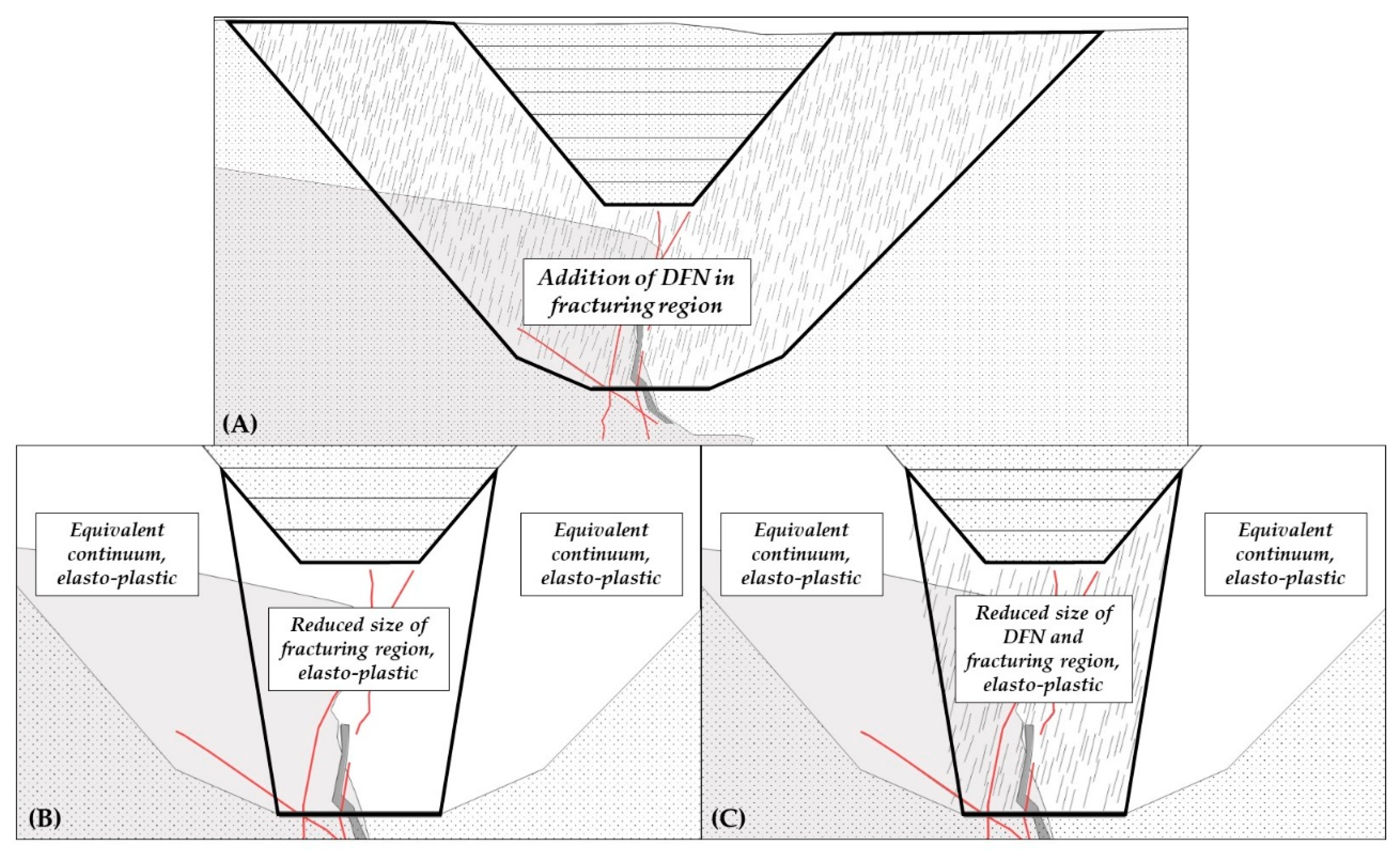
Figure 11.
FDEM geometry variations for (A) model No. 6, (B) model No. 7, and (C) model No. 8.

Figure 12.
ELFEN deletion methodology and model production over time. Model time is adjusted for comparison between models, with the common point being the onset of active cave propagation (first deletion).
Figure 12.
ELFEN deletion methodology and model production over time. Model time is adjusted for comparison between models, with the common point being the onset of active cave propagation (first deletion).

Figure 13.
FDEM model results after 8900 m2 ± 1% material removed. Maximum XY displacement at the toe of the pit slopes, maximum Y displacement representing height of draw (HOD), and model times past first deletion are reported for each model.
Figure 13.
FDEM model results after 8900 m2 ± 1% material removed. Maximum XY displacement at the toe of the pit slopes, maximum Y displacement representing height of draw (HOD), and model times past first deletion are reported for each model.

Figure 14.
FDEM model results for models No. 1 and No. 6 after 8900 m2 ± 1% material removed. Maximum XY displacement contours. Developed cave shape comparison defined by 10 m vertical displacement.
Figure 14.
FDEM model results for models No. 1 and No. 6 after 8900 m2 ± 1% material removed. Maximum XY displacement contours. Developed cave shape comparison defined by 10 m vertical displacement.

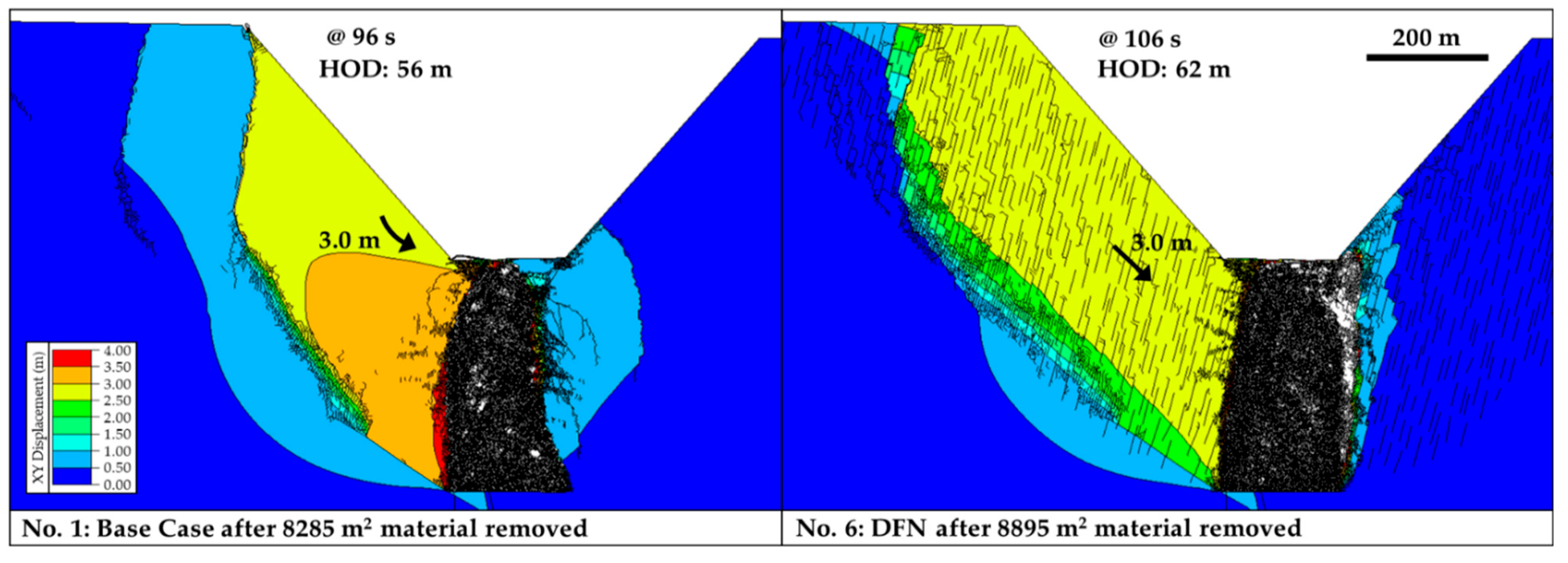
Figure 15.
FDEM model results for models No. 1 and No. 6 with similar displacement in left pit wall. Maximum XY displacement contours.
Figure 15.
FDEM model results for models No. 1 and No. 6 with similar displacement in left pit wall. Maximum XY displacement contours.

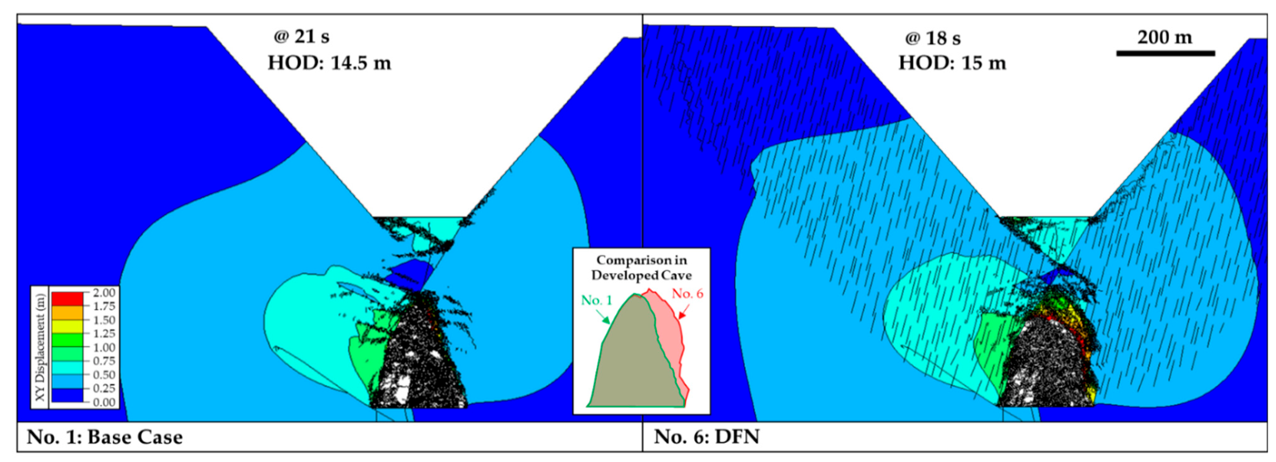
Figure 16.
FDEM model results for models No. 1 and No. 6 after 1450 m2 ± 1% material removed. Maximum XY displacement contours. Developed cave shape comparison defined by 1 m vertical displacement.
Figure 16.
FDEM model results for models No. 1 and No. 6 after 1450 m2 ± 1% material removed. Maximum XY displacement contours. Developed cave shape comparison defined by 1 m vertical displacement.


Table 1.
Confidence level targets by project stage (data after [13]).
Table 1.
Confidence level targets by project stage (data after [13]).
| Project Stage | |||||
|---|---|---|---|---|---|
| Project Level Status | Conceptual | Prefeasibility | Feasibility | Design and Construction | Operations |
| Geotechnical Characterization | Regional data compilation | Local scale data compilation and assessment | Ongoing collection of new local scale data | Improvement of database and 3D model | Continued refinement and maintenance of database and 3D model |
| Target levels of data confidence for each model | |||||
| Geology | >50% | 50–70% | 65–85% | 80–90% | >90% |
| Structural | >20% | 40–50% | 45–70% | 60–75% | >75% |
| Hydrogeological | >20% | 30–50% | 40–65% | 60–75% | >75% |
| Rock mass | >30% | 40–65% | 60–75% | 70–80% | >80% |
| Geotechnical | >30% | 40–60% | 50–75% | 65–85% | >80% |
Table 2.
2D FDEM modelling scenarios.
| Model No. | Description |
|---|---|
| 1 | Base case pit-to-cave transition. |
| 2 | Undercut level initiation on left side and reversed draw sequencing. |
| 3 | Symmetric draw sequence. |
| 4 | Fault to the left of the undercut level removed. |
| 5 | Symmetric draw sequence, fault to the left of the undercut level removed. |
| 6 | Discrete fabric structures introduced in fracturing region with coupled DFN model. |
| 7 | Reduced size of fracturing region. |
| 8 | Discrete fabric structures introduced in fracturing region with coupled DFN model of reduced size. |
| 9 | No open pit. |
Table 3.
Geotechnical domain properties and FDEM modelling input parameters.
| Parameter | Unit | Value | Source | ||
|---|---|---|---|---|---|
| Volcanics | Sediments | Monzonite | |||
| Intact | |||||
| UCS, σci | MPa | 121 | 99 | 123 | Lab value |
| Young’s Modulus, Ei | GPa | 67.7 | 68.0 | 65.0 | Lab value |
| Hoek–Brown material constant, mi | - | 18.9 | 12.0 | 19.7 | Lab value |
| Tensile strength, σt | MPa | 6.4 | 8.3 | 6.2 | Generalized Hoek–Brown |
| Poisson’s ratio, ν | - | 0.27 | 0.28 | 0.26 | Lab value |
| Rock mass | |||||
| GSI | - | 63 | 48 | 78 | Field estimate |
| Young’s Modulus, Erm | GPa | 38.6 | 17.8 | 55.3 | Generalized Hoek–Diederichs [57] |
| Density, ρ | kg m−3 | 2880 | 2880 | 2880 | Lab value |
| Tensile strength, σtm | MPa | 3.0 | 2.3 | 4.1 | Mohr–Coulomb Criteria |
| Cohesion, c | MPa | 4.1 | 2.5 | 6.2 | Generalized Hoek–Brown |
| Friction, φ | degrees | 49.8 | 40.0 | 53.7 | Generalized Hoek–Brown |
| Fracture energy, Gf | J m−2 | 12.8 | 21.0 | 12.7 | [58] |
| Dilation, ψ | degrees | 6 | 5 | 13 | [59] |
| Discontinuities | Faults | Joints and newly generated fractures | |||
| Fracture cohesion, c | MPa | 0.6 | 0 | Lab value | |
| Fracture friction, φ | degrees | 17 | 31 | Lab value | |
| Normal stiffness, kn | GPa m−1 | 5 | 5 | [16] | |
| Shear stiffness, ks | GPa m−1 | 0.5 | 0.5 | [16,54] | |
| Stress level | |||||
| In situ stress ratio, K | - | 2 | Conceptual | ||
Table 4.
ELFEN model stages and time step controls.
| Stage | Duration (s) | Number of Stages | Time Step Control Data | |||
|---|---|---|---|---|---|---|
| Initial Time Step (s) | Max Time Step (s) | Max Change (%) | Factor of Critical Timestep | |||
| Equilibrium | 2 | 1 | 1e-5 | 1 | 101 | 0.75 |
| Pit Excavation | 2 | 8 | ||||
| Post-pit Equilibrium | 2 | 1 | ||||
| Undercut Excavation | 5 | 3–5 | ||||
| Initial Cave Propagation | 5 | 1 | ||||
| Active Cave Propagation (with deletion) | 10–30 | 9 | ||||
Table 5.
Comments concerning the results of the conceptual pit-to-cave models.
| Purpose of Model (Test) | Related Models 1 | Description of Results |
|---|---|---|
| Direction of undercut level excavation and draw | 2, 3, 5 | Mine design parameters, such as the direction of the draw, do not significantly impact the magnitude of deformation observed in the left pit wall relative to other scenarios. Reversed draw (No. 2) resulted in the development of a tension crack in a similar location, while the slope deformation decreased, despite an increased HOD. The symmetric draw resulted in a tension crack forming lower in the pit wall. Cave shapes with reversed and symmetrical draws were more centralized, while the base case model showed propagation skewed to the left despite the deformation of the left slope pushing the cave to the right. The effect of the slope deformation pushing the cave development to the right can be seen in model No. 3 due to the symmetrical draw. Reversed draw required a longer model run time to extract the same amount of material, while symmetric draw negligibly impacted the run time. |
| Fault connection between pit and cave | 4, 5 | The pit wall deformation decreased significantly in the absence of the fault providing a connection between the pit walls and undercut level. The formation of tension cracks still occurred to release strain due to the deformation in the left pit wall from dilation at the contact of the stiff volcanics overlying the softer sedimentary units. Symmetric draw sequencing affected both the model run time and the HOD at a greater rate without the fault present. Cave shapes were more centralized due to the decrease in deformation, similar to the shape of the developed caves in the models with reversed and symmetric draws (No. 2 and 3). |
| Inclusion of DFN | 6, 8 | Inclusion of a DFN within the full fracturing zone (No. 6) resulted in a decrease in the deformation within the pit wall but an increase in the deformation on the crest due to the connection between the fault on the left side of the undercut level and surface through the joint network. Cave propagation is influenced by the orientation of the DFN fabric. Model No. 1 (no DFN) shows the equivalent deformation to No. 6 (with DFN) along the pit slope, but the deformation is achieved for smaller HOD (Figure 14). Note that the DFN includes fractures with sizes of ~50 m and spacings of ~10–15 m, and therefore it does not impact the assigned GSI values. However, the anisotropy effect on the models is significant regarding the deformation mechanism, magnitude of deformation behind the pit crest, and the cave development shape. In model No. 8, where the fracturing area and DFN area were reduced, the deformation magnitudes at the right pit toe are doubled. |
| Scale of fracturing regions | 7, 8 | Limiting the fracturing region to the cave area alone removes the mechanisms of deformation associated with the pit-to-cave transition; however, as seen in No. 7, it has the equivalent effect of removing the fault at the left side of the UCL. HOD for No. 7 was more comparable to the model without the open pit (No. 9). A noticeable change in the shape of the developed cave on the left side could be attributed to the decrease in deformation pushing the cave to the right near the pit toe. The inclusion of the DFN in the smaller fracturing area resulted in less change between cave shape and HOD (comparing No. 8 to No. 6), which may indicate that the inclusion of the DFN can better capture caving characteristics even with limiting fracturing to the cave area. However, the deformation magnitudes are different on either toe of the slope, and the impact of the fault on the left of the UCL is neglected. |
| Caving without an open pit | 9 | There is no significant effect of the pit on the cave propagation rate or shape, despite a slight increase in HOD in No. 9. While no equivalent model to No. 9 has been run with a DFN included, it is expected that the confinement would result in less impact from the fabric anisotropy. |
1 Base case model (No. 1) used for all comparisons.
Publisher’s Note: MDPI stays neutral with regard to jurisdictional claims in published maps and institutional affiliations. |
© 2022 by the authors. Licensee MDPI, Basel, Switzerland. This article is an open access article distributed under the terms and conditions of the Creative Commons Attribution (CC BY) license (https://creativecommons.org/licenses/by/4.0/).
Share and Cite
MDPI and ACS Style
Shapka-Fels, T.; Elmo, D. Numerical Modelling Challenges in Rock Engineering with Special Consideration of Open Pit to Underground Mine Interaction. Geosciences 2022, 12, 199. https://doi.org/10.3390/geosciences12050199
AMA Style
Shapka-Fels T, Elmo D. Numerical Modelling Challenges in Rock Engineering with Special Consideration of Open Pit to Underground Mine Interaction. Geosciences. 2022; 12(5):199. https://doi.org/10.3390/geosciences12050199
Chicago/Turabian StyleShapka-Fels, Tia, and Davide Elmo. 2022. "Numerical Modelling Challenges in Rock Engineering with Special Consideration of Open Pit to Underground Mine Interaction" Geosciences 12, no. 5: 199. https://doi.org/10.3390/geosciences12050199
Note that from the first issue of 2016, this journal uses article numbers instead of page numbers. See further details here.