Review

Back to the Future: Using Long-Term Observational and Paleo-Proxy Reconstructions to Improve Model Projections of Antarctic Climate

by
Thomas J. Bracegirdle
1,*,
Florence Colleoni
2,
Nerilie J. Abram
3,
Nancy A. N. Bertler
4,
Daniel A. Dixon
5,
Mark England
6,
Vincent Favier
7,
Chris J. Fogwill
8,
John C. Fyfe
9,
Ian Goodwin
10,
Hugues Goosse
11,
Will Hobbs
12,
Julie M. Jones
13,
Elizabeth D. Keller
14,
Alia L. Khan
15,
Steven J. Phipps
16,
Marilyn N. Raphael
17,
Joellen Russell
18,
Louise Sime
1,
Elizabeth R. Thomas
1,
Michiel R. van den Broeke
19 and
Ilana Wainer
20
add Show full author list remove Hide full author list
1
British Antarctic Survey, Cambridge CB3 0ET, UK
2
Istituto Nazionale di Oceanografia e Geofisica Sperimentale, 34010 Sgonico (TS), Italy
3
Research School of Earth Sciences and ARC Centre of Excellence for Climate Extremes, Australian National University, Canberra ACT 2601, Australia
4
Antarctic Research Centre, Victoria University of Wellington, Wellington 6140, New Zealand
5
Climate Change Institute, University of Maine, Orono, ME 04469, USA
6
Applied Physics and Applied Mathematics Department, Columbia University, New York, NY 10027, USA
7
Centre national de la Recherche Scientifique, Univ. Grenoble Alpes, Institut des Géosciences de l’Environnement (IGE), 38000 Grenoble, France
8
School of Geography, Geology and the Environment, Keele University, Staffordshire ST5 5BG, UK
9
Canadian Centre for Climate Modelling and Analysis, Environment and Climate Change Canada, Victoria, BC V8W 2Y2, Canada
10
Marine Climate Risk Group, Department of Environmental Sciences, 12 Wallys Walk, Macquarie University, Sydney NSW 2109, Australia
11
Earth and Life Institute, Université Catholique de Louvain, 1348 Louvain-la-Neuve, Belgium
12
Antarctic Climate and Ecosystems Cooperative Research Centre (ACE CRC), University of Tasmania, Tasmania 7001, Australia
13
Department of Geography, University of Sheffield, Sheffield S10 2TN, UK
14
GNS Science, 30 Gracefield Rd, Gracefield 5010, PO Box 31-312, Lower Hutt 5040, New Zealand
15
Department of Environmental Sciences, Western Washington University, Bellingham, WA 98225, USA
16
Institute for Marine and Antarctic Studies, University of Tasmania, Hobart TAS 7001, Australia
17
Department of Geography, UCLA, Los Angeles, CA 90095, USA
18
Department of Geosciences, University of Arizona, Tucson, AZ 85721, USA
19
Institute for Marine and Atmospheric Research, Utrecht University, 3584 CC Utrecht, The Netherlands
20
Oceanography Institute, University of São Paulo, São Paulo 05508-120, Brazil
*
Author to whom correspondence should be addressed.
Geosciences 2019, 9(6), 255; https://doi.org/10.3390/geosciences9060255
Submission received: 15 May 2019 / Revised: 31 May 2019 / Accepted: 4 June 2019 / Published: 7 June 2019

Abstract

:
Quantitative estimates of future Antarctic climate change are derived from numerical global climate models. Evaluation of the reliability of climate model projections involves many lines of evidence on past performance combined with knowledge of the processes that need to be represented. Routine model evaluation is mainly based on the modern observational period, which started with the establishment of a network of Antarctic weather stations in 1957/58. This period is too short to evaluate many fundamental aspects of the Antarctic and Southern Ocean climate system, such as decadal-to-century time-scale climate variability and trends. To help address this gap, we present a new evaluation of potential ways in which long-term observational and paleo-proxy reconstructions may be used, with a particular focus on improving projections. A wide range of data sources and time periods is included, ranging from ship observations of the early 20th century to ice core records spanning hundreds to hundreds of thousands of years to sediment records dating back 34 million years. We conclude that paleo-proxy records and long-term observational datasets are an underused resource in terms of strategies for improving Antarctic climate projections for the 21st century and beyond. We identify priorities and suggest next steps to addressing this.

1. Introduction

Making quantitative projections of how Antarctic climate may change over the 21st century and beyond involves the use of numerical climate models. Trust in the climate models used to make projections is based largely on evaluation against observable features of the climate system [1]. In this context it is important to consider a range of model-observation metrics across different components of the climate system. Although rigorous evaluation of many key aspects of climate models’ performance is possible based on modern observational datasets, limiting factors in model evaluation for Antarctica and the Southern Ocean are the short time period spanned by modern in-situ instrumental datasets and the lack of sustained observations of some key processes [2]. In particular in Chapter 9 of the Intergovernmental Panel on Climate Change (IPCC) Fifth Assessment Report (AR5) [1] it is stated that ‘In many cases, the lack or insufficient quality of long-term observations, be it a specific variable, an important process, or a particular region (e.g., polar areas, the upper troposphere/lower stratosphere (UTLS), and the deep ocean), remains an impediment’ to model evaluation.
A key challenge when interpreting projections of 21st century climate change is the wide range of estimated changes, even when the same anthropogenic emissions forcing scenario is used [3]. Over many parts of the planet these changes scale with global warming rate, i.e., climate models that have a high sensitivity in terms of their global response to anthropogenic forcing also have a high sensitivity in a given region or continent. However, this is not the case for Antarctica and the Southern Ocean, where, for projections to 2100, a high sensitivity model globally is not necessarily a high sensitivity model over Antarctica (e.g., [4,5]). This points to a major role for regional processes in modulating climate and ice sheet changes over Antarctica. The implication is that our estimates of future Antarctic climate change and its global impacts are strongly reliant on good representation of the atmosphere-ocean-ice system of Antarctica and the Southern Ocean [6].
Here we define the start of the modern observational era as the introduction of a network of continuous meteorological observation stations over Antarctica during the International Geophysical Year (IGY) in 1957/58. However, recognizing that a major improvement occurred subsequently with the introduction of high-quality continuous satellite remote sensing data in 1978/79, we further identify the post 1978/79 period as the modern satellite era. We explore the potential to use longer-term pre-modern (i.e., pre-1957/58) instrumental climate reconstructions and paleoclimate proxies to help improve the reliability of model projections of Antarctic climate change under future emission scenarios to the year 2100. This is a broad time span that incorporates a range of data sources, from early twentieth century in-situ instrumental observations (terrestrial and ship-based platforms) to paleo-climate proxies of different past periods of relevance to projections. In the context of using longer-term datasets to contribute to climate model evaluation, here we outline the current state-of-the-art datasets, identify the key current challenges relevant to model evaluation, and then suggest next steps to addressing these challenges. This paper is novel in the sense that we consider a wide range of different types of long-term datasets, and in each case consider specifically the relevance for informing climate model projections.
This paper draws from discussions at the 2018 Past2Projections workshop of Antarctic Climate Change in the 21st Century (AntClim21), a scientific research program of the Scientific Committee on Antarctic Research (SCAR). AntClim21 is focused on improving estimates of how Antarctic and Southern Ocean climate may change over the 21st century. Due to the wide range of timescales and scientific priorities discussed at the workshop, this paper is divided into three main sections. Preceding these, Section 2 introduces key phenomena and processes to provide background for the main sections. Section 3 focusses on past climatic states and transitions back to the presumed onset of the Antarctic glaciations, 34 million years before present. Section 4 covers the last two millennia, considered as the baseline climate of modern conditions, since this matches the approximate range of a number of prominent reconstruction and modelling initiatives. Section 5 looks at the emergence of anthropogenic climate signals and the potential for using what we have observed about the response of the climate system to present levels of anthropogenic forcing to help inform estimates of future change. Section 3 and Section 4 follow a similar structure, whereby they include an outline of the current state-of-the-art datasets, the identification of key current challenges relating to model evaluation, followed by suggested next steps. Section 5 focusses on the specific topic of the emergence of anthropogenic climate change signals.

2. Key Phenomena and Processes Relating to Past Reconstructions and Future Projections of Antarctic Climate

There are a number of phenomena and processes that are important in both the design and interpretation of many longer-term datasets of the Antarctic ocean-atmosphere-ice system. These will be mentioned widely in this paper, and are therefore introduced only briefly here.
From an atmospheric point of view, variability in circulation is widely characterized by indices of the Southern Annular Mode (SAM), which is the leading mode of Southern Hemisphere (SH) atmospheric variability in sea-level pressure [7]. The SAM captures variations in the latitude and/or speed of the Southern Ocean westerlies with more positive index values associated with more poleward and/or stronger westerlies. More regionally, an important feature of atmospheric variability is the Amundsen Sea Low (ASL) [8]. The ASL is a climatological low-pressure anomaly adjacent to West Antarctica, the depth of which is in fact related to the SAM [8]. However, it is a key part of understanding atmospheric circulation influences on regional weather and climate over large parts of West Antarctica and the Antarctic Peninsula and is important in the context of understanding the effects of both stratospheric ozone depletion and tropical variability. With regard to effects of ozone depletion, some model studies indicate that the ozone hole has acted to deepen the ASL [9,10]. The mechanisms responsible for simulated ASL sensitivity to the ozone hole are not well known, but one suggestion is that ozone-depletion-related circumpolar storm track changes cause an increase in cyclonic activity over the Amundsen Sea and a deeper ASL [10]. In relation to the remote influence of tropical variability and trends, the ASL is situated to the poleward end of a pattern of high and low atmospheric pressure anomalies that connects the Tropical Pacific and the Amundsen Sea. This pattern, known as the Pacific South American (PSA) pattern, is strongest in austral winter and emerges as the second mode of SH atmospheric variability. The PSA is generally explained as a Rossby wave train propagating from the tropical Pacific towards West Antarctica [11] and therefore provides a key mechanism for explaining Antarctic teleconnections to El Niño–Southern Oscillation (ENSO). The PSA, SAM and ASL have been found to be sensitive to external climate forcing (both natural and anthropogenic), with stratospheric ozone depletion/recovery, greenhouse gases, orbital parameters, solar forcing and volcanic activity, all potentially important depending on the time period and season under consideration [10,12,13,14,15,16].
In addition to the dynamic influence of atmospheric circulation patterns described above, climate conditions over the Antarctic continent are also influenced thermodynamically by changes in surface conditions over the Southern Ocean (i.e., sea-surface temperature (SST) and sea ice extent/concentration)—particularly on centennial and longer timescales [6,17,18]. This is particularly apparent for Antarctic-wide averages of precipitation/surface mass balance (SMB) and surface temperature.
From an oceanic point of view, Antarctica is surrounded by the eastward-flowing Antarctic Circumpolar Current (ACC). Branches of the ACC yield two main Southern Ocean polar gyres, the Weddell Sea gyre (Atlantic sector), and the Ross Sea gyre (Pacific sector). At depth, the ACC is composed of Circumpolar Deep Water (CDW), a warm (~0.5 to 1.5 °C close to the margins) and relatively salty water mass (~34.8 PSU). Part of the CDW is geostrophically adjusted and forms the westward-flowing Antarctic Slope Current (ASC), that impinges the continental shelf edge around Antarctica [19]. On the continental shelf edge, brine rejection from sea ice formation and cooling by cold air flowing off the continent yields cold dense bottom waters that contribute to Antarctic Bottom Water (AABW) formation. In the Bellingshausen and Amundsen Seas, the ASC is weak and CDW can flow onto the continental shelf. On the shelf, this relatively warm water, mixed with local continental shelf waters, flows under the Antarctic ice shelves and causes sub-shelf melting that forms the local Ice Shelf Water (ISW). The ISW flows out to the continental shelf edge as one of the contributors to AABW formation. ISW, CDW/ASC, bottom waters and AABW all have distinct signatures in terms of fauna and mineral composition of sediments. Thus, sediment cores can provide information on water mass pathways in past climates.

3. Past Climates and Transitions (34 Ma to the Last 2 Ka)

The potential of paleoclimate studies in the context of climate model evaluation and improving projections resides in the necessity to simulate projected climate states substantially different from present-day [20]. Long-term paleoclimate records can thus be used to frame valuable tests for climate models across a range of climate states back to the presumed onset of glaciation of the Antarctic ice sheet during the Eocene/Oligocene Transition (~34 million years ago, Ma, EOT) [21]. They can help to improve understanding of mechanisms that drive variability and changes in Antarctic climate. The question of how to bound a conceptual future with realistic but uncertain paleoclimate modeling and observational reconstructions is central to the evaluation of the climate models used to carry out projections [22].

3.1. Current State-of-the-Art

Key periods of both direct and indirect relevance to improving climate projections are (Table 1): the Holocene (from ~11.7 thousand years ago, ka), the Last Glacial Maximum (LGM) (21 ka), the Last Great Interglacial (LIG, 115–130 ka, marine isotope stage (MIS) 5), MIS 11 (374–424 ka), the mid Pliocene Warm Period (mPWP) (3–3.3 Ma), the mid Miocene Climatic Optimum (MMCO) (14–17 Ma) and the EOT (~34 Ma). These periods are characterized by a gradual increase in atmospheric CO2 looking back through time (Figure 1) and are relevant to Antarctic projections specifically in relation to the impact of oceanic warmth on the stability of marine-based Antarctic ice sheet; the seasonality of sea ice cover; bottom water formation and related oceanic heat transport; changes in pole-to-equator thermal gradients and atmospheric jet streams.
Simulating past climates implies, as for present climates, a data-model comparison approach to evaluate the climate reconstructions and identify potential biases that do not arise in short-term 20th century simulations [20]. Over the past decades various model inter-comparison initiatives, most of them still on-going, have been actively supported by the paleoclimate community:
-
the Paleoclimate Model Intercomparison Project (PMIP, now in phase 4, and endorsed in the current World Climate Research Programme’s Coupled Model Intercomparison Phase 6 (CMIP6) project [23]): equilibrium simulations of the mid-Holocene (~6 ka, [24]), the LGM [25] and the LIG [26]. The last two phases also include the last millennium and the current phase is aimed at simulating transient evolution of particular time windows such as the last deglaciation of the LIG.
-
The Pliocene Model Intercomparison Project (PlioMIP, now in phase 2, [27]): equilibrium run with averaged conditions of the mPWP. Phase 2 includes equilibrium or transient simulations of specific glacial-interglacial oscillations within the mPWP.
-
The Pliocene Ice Sheet Model Intercomparison Project (PLISMIP-ANT, [28]): equilibrium simulations to test the sensitivity of the Antarctic ice sheet to the Pliocene warmth, forced with the outputs of PlioMIP experiments.
-
The Miocene Model Intercomparison Project (MioMIP, starting 2019): equilibrium simulations of particular snapshots centered on the MMCO and on the late Miocene.
-
The Deep-time Model Intercomparison Project (DeepMIP, [29]): is on-going and tests the sensitivity of models to very high atmospheric CO2 concentrations and/or different paleo-geographies, as suggested by proxy reconstructions for times older than the EOT.
These initiatives have triggered the development of paleoclimate proxy databases focused on those specific periods. For example, a multi-proxy database of sea surface temperature for the LGM was compiled as part of the Multiproxy Approach for the Reconstruction of the Glacial Ocean surface (MARGO) project [30]. For the LIG, two main databases have been compiled, the first one includes terrestrial and marine sites [31] and the second one includes high-latitudes ice cores and marine sediment cores [32]. The most complete global reconstruction of climate is currently the Pliocene Research, Interpretation and Synoptic Mapping (PRISM) dataset [33]. For the deep past, Miocene, EOT and before, no similarly comprehensive databases exist, mainly due to a scarcity of data. For past global to regional sea level changes, paleo-sea level markers for all the periods mentioned above are being compiled as part of the PALeo constraints on SEA level rise working group (PALSEA).
Relevance for improving projections:
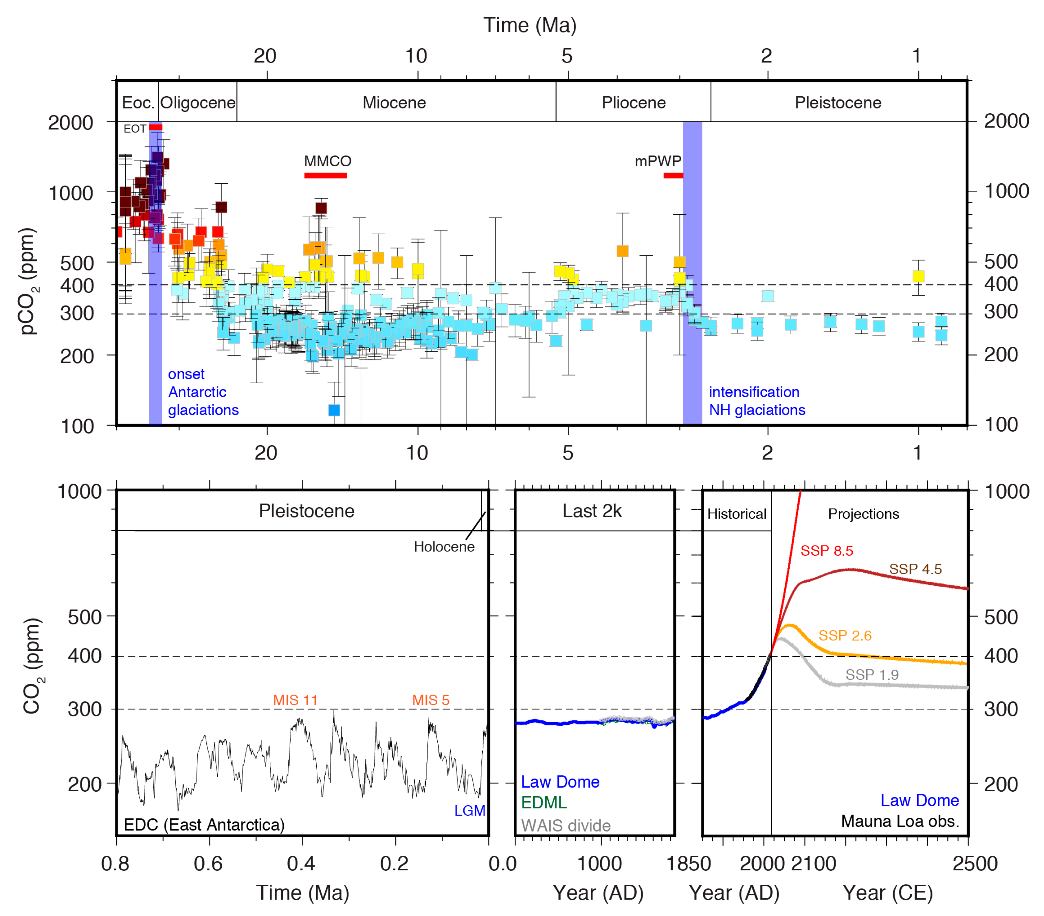
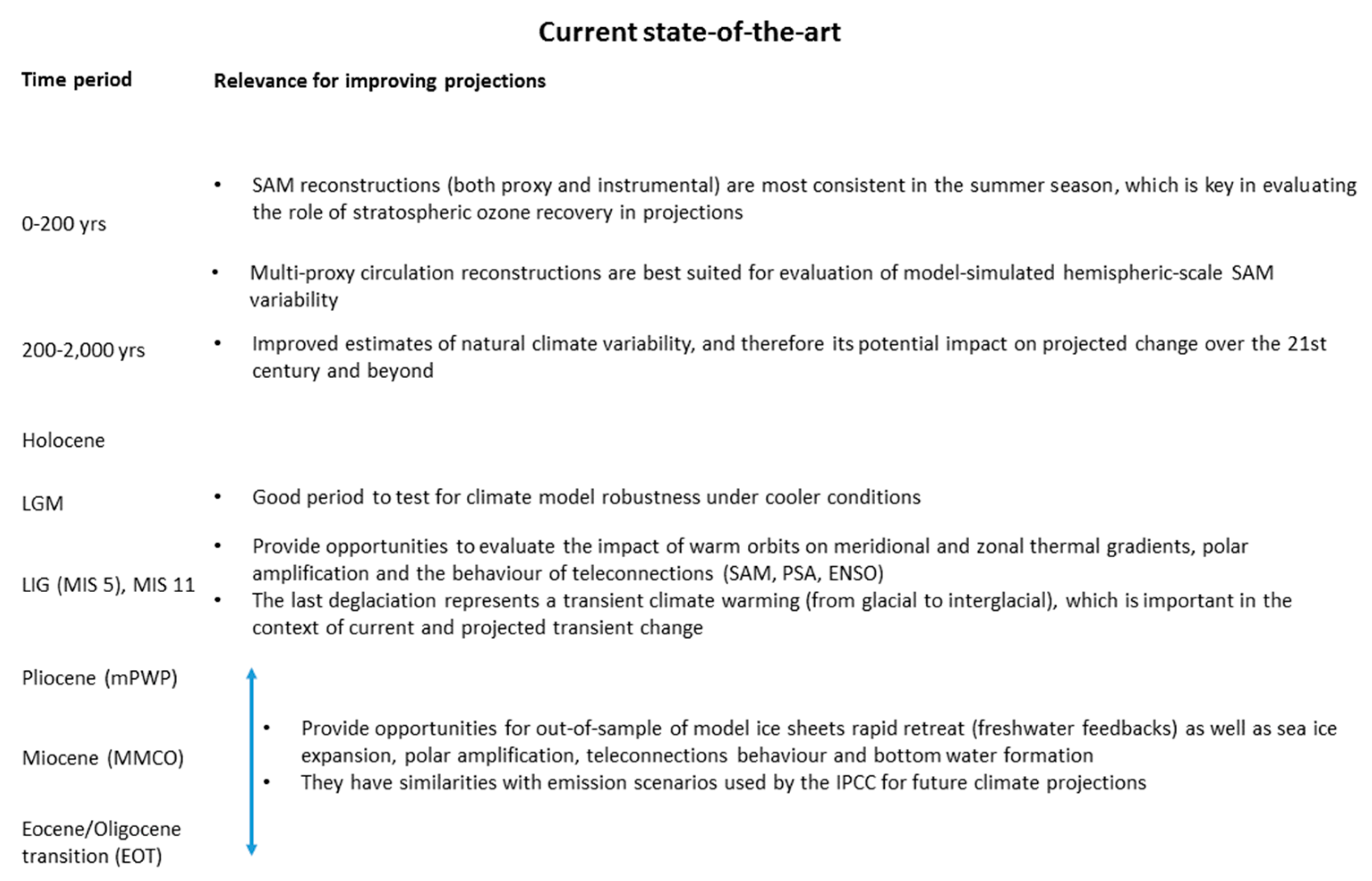
  • The last deglaciation represents a transient climate warming (from glacial to interglacial) with atmospheric CO2 remaining lower than present day (< 300 ppm, Figure 1).
  • The LIG and MIS 11 can be used to evaluate the impact of warm orbits on meridional and zonal thermal gradients, polar amplification and the behaviour of teleconnections (SAM, PSA, ENSO). Both periods are suitable for reconstructing the oceanic conditions leading to Marine Ice Sheet Instability in Antarctica under low atmospheric CO2 concentration [34].
  • mPWP, MMCO and EOT provide opportunities for out-of-sample evaluation of the ability of models to simulate rapid retreat of ice sheet (freshwater feedbacks) as well as sea ice expansion, polar amplification, teleconnections behaviour and bottom water formation. They have similarities with emission scenarios used by the IPCC for future climate projections.

3.2. Current Challenges

In order to accurately simulate past climates, it is important to have reliable reconstructions of atmospheric greenhouse gas concentrations on a range of time scales. Atmospheric concentrations of CO2 can be retrieved from Antarctic ice core records back to about 850 ka (e.g., [36]) (Figure 1). However, a recent study shows that uncertainties in CO2 reconstruction of the Late Pleistocene are non-negligible [59], leading to large differences between models, especially in the case of ice sheet glaciation and deglaciation thresholds [60]. For pre-ice-core records, CO2 reconstructions are retrieved from sediment cores, with large uncertainties (Figure 1, e.g., [39]). The low temporal resolution of CO2 records, ice cores included, is therefore a major challenge in terms of accurately modeling past millennial to sub-millennial time-scale CO2-forced climate variability.
In addition to the importance of a reliable greenhouse gas forcing history, climate models also need to be set up with accurate boundary conditions. A current challenge in this respect is paleo-bathymetry, which is critical to the understanding and reconstruction of past ocean circulation and marine-based ice sheet dynamics. For ice sheets, improved knowledge of bathymetry can help to reconstruct the occurrence of pinning points favoring the stability of the ice sheet and formation of ice shelves [43,61]. For the ocean, it helps to more realistically simulate regional circulations, the formation of AABW and heat exchange across the continental shelf edge (e.g., [62]). Paleo-morphological features of current bathymetry can be used to infer the type of ice sheet flow, the occurrence and pathways of release of meltwater [63], pathways of bottom water formation and feedbacks with surrounding oceanic water masses. The scarcity of marine deep drilling sites hampers accurate dating of the paleo-bathymetry reconstructions based on seismic stratigraphy (e.g., [64]) and thus limits the availability of reliable reconstructions to be used as boundary conditions in models [61].
Challenges relating to forcing history and boundary conditions are relevant to the long-standing issue of climate model spin-up, which remains difficult to solve. A climatic state at a given time results from the superposition of long-term (several millennia to tens of millennia mostly influenced by astronomical forcing) and short-term climate evolution prior to that moment. From a modelling perspective, simulating the long-term transient evolution of the entire system is only doable for a limited range of simplified climate models, such as Earth System Models of Intermediate Complexity (EMICs) [65,66], or very low-resolution Earth System Models (ESMs) (e.g., [67]). Some studies suggest that ~5,000 years of free running, initialized with fixed conditions (e.g., a climatology of ocean state variables), might be required to adequately spin up the deep ocean, particularly for climates which are significantly different to present (e.g., [68]). This is especially true for much colder periods like the LGM or much warmer periods such as the mPWP, the MMCO or the EOT. Therefore, depending on the model used and the spin-up method and duration, different equilibria can be reached for a single climate state (e.g., [69]). For example, in some models, more than 3000 years of spin-up are necessary to trigger the realistic formation of AABW under glacial climatic conditions [70].
Turning to challenges of data-model comparisons in specific phenomena or variables, key issues have been revealed in analyses of the simulations conducted by the various model intercomparison projects. Comparison of PMIP3 simulations of the LIG with reconstructions reveals that the models are unable to capture the reconstructed warmth at high latitudes, particularly in the Southern Ocean (e.g., [26,71]). Simulations suggest that models overestimate the sea ice extent as well as the upwelling in some cases. Conversely, models are found to underestimate the Antarctic cooling in LGM simulations [72]. This has implications for the reliability of simulated westerlies, which are however difficult to assess in models due to uncertainties in available proxies for westerlies in the LGM [5,73,74]. Similar issues have been noted in PlioMIP experiments of the mPWP for which model disagreements in Southern Ocean SST, sea ice extent, westerly winds and the broader thermohaline circulation are again difficult to assess due to uncertainty in proxy reconstructions across these variables [75]. However, looking in more detail at processes, PlioMIP simulations show that there is a mismatch between proxy and simulated deep water ventilation in the Southern Ocean. Only a few models are able to explain the reconstructed changes in AABW fluctuations during the mPWP [70]. In general, data-model mismatches in the Southern Ocean are likely due, at least in part, to the omission of key processes within the climate models, such as the discharge of Antarctic meltwater into the ocean [71] or incorrect formation mechanisms for Antarctic bottom water [76].
Another current challenge potentially responsible for model-data differences is temporal consistency between paleo-proxy data and model output. For example, the PRISM dataset collated proxies over the entire mPWP [33,50] while models participating to the PlioMIP project had to impose specific sub-periods for their simulations [77]. This discrepancy contributed to a mismatch between the PRISM proxy database and the simulations [78]. Model intercomparison projects now attempt to focus on specific time slices (e.g., PMIP, PlioMIP2 and MioMIP). There is therefore a requirement to retrieve geological archives of at least sub-orbital to millennial temporal resolution and calibrate the large range of age models across the various types of proxies and regions for the Pliocene (e.g., [78,79]) and also other periods of interest. Another timing-related issue is the seasonal nature of many proxies. Some proxies have inherent biases toward a specific season or can be representative of mean annual conditions.
Relevance for improving projections:
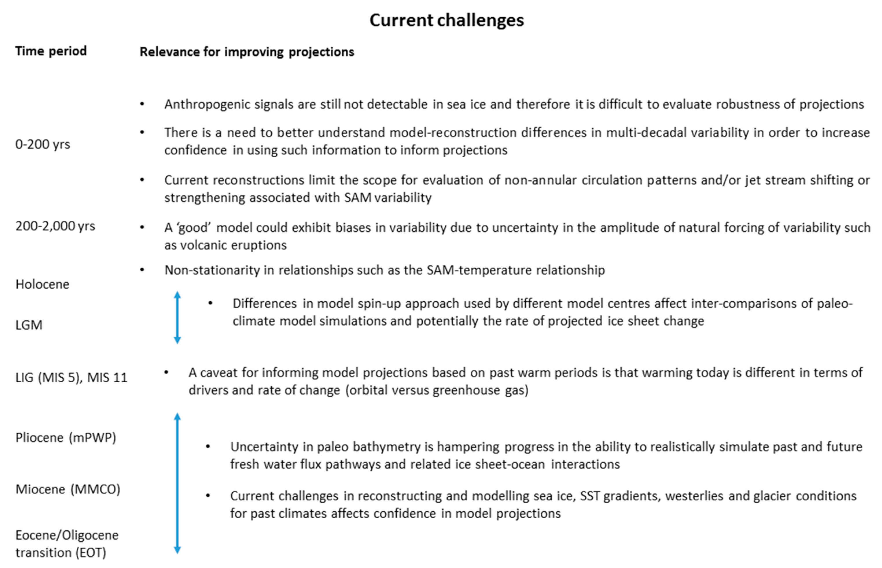
  • Uncertainty in paleo bathymetry is hampering progress in the ability to realistically simulate past and future fresh water flux pathways and related ice sheet-ocean interactions
  • Differences in model spin-up approach used by different model centres affect inter-comparisons of paleo-climate model simulations and potentially the rate of projected ice sheet change
  • Current challenges in reconstructing and modelling sea ice, SST gradients, the ocean thermohaline circulation, westerlies and glacier conditions for past climates affects confidence in model projections
  • A caveat for informing model projections based on past warm periods is that warming today is different in terms of drivers and rates of change (orbital versus greenhouse gas)

3.3. Next Steps

Paleoclimate model intercomparison projects (PMIPs) have increasingly provided data and stimulated the development of approaches for using paleoclimate simulations to improve future projections [20,80]. Examples of promising approaches that combine output from PMIP simulations and long-term climate reconstructions to constrain Antarctic climate projections include: (i) exploiting Antarctic/global warming relationship [81], (ii) utilizing cross-model correlations in simulated future and past sea ice extent (SIE) changes [81], and (iii) by assessing links between SIE and the circumpolar surface westerlies as simulated by models in a range of different past climates [73]. A key next step that would benefit the above interpretations by, for example, increasing the statistical significance of relationships across the multi-model ensemble, would be to increase the number of modelling groups participating in future PMIPs (only nine models were available for use in recent PMIP3 studies [73,81]).
Recent studies have used Antarctic ice sheet contributions to mPWP and LIG global mean sea levels as tuning targets for ice sheet models to reduce the uncertainties on sea level projections [82,83]. Further investigations of Antarctic ice sheet sensitivity to past warm climate conditions (e.g., MMCO, [51]; mPWP, [28,84]; LIG, [85], and the last deglaciation, [86]) are needed to better constrain its tipping points under different level of atmospheric CO2 concentration (Figure 1).
Increases in computing power now make it more feasible to run transient simulations of a few thousands of years with fully coupled Earth System Models, as for example for the LIG in the framework of PMIP4 [24]. A recent on-going German initiative, Paleoclimate Modeling (PALMOD), is aimed at simulating the entire last glacial cycle (130–0 ka) with ESMs. Implementation of adaptive mesh and unstructured grids for models to optimize the use of computing resources while reaching high resolution in areas of interests is on-going. Improvements in computing facilities are nevertheless needed to increase spatial resolution of ESMs or to allow for high resolution coupled regional downscaling. Evaluation of such models for the past will require increases in temporal resolution and better characterization of age model uncertainty in marine and ice core proxies to better identify and constrain local polar processes and feedbacks that are still missing in models, as for example processes at the interface between ice dynamics, sea ice, ocean, and atmosphere [61,87]. One on-going project, Pliocene climate variability over glacial-interglacial timescales (PlioVAR), is aimed at collecting and referencing sediment cores with potential for millennial to sub-millennial time resolution.
In addition to increased temporal resolution, it is necessary to select key variables that can ideally be both easily retrieved in the available proxy or observational datasets and are also representative of the main features of a given climate state such as global mean seasonal temperature, inter-hemispheric temperature gradients, polar amplification, cryosphere conditions, and the carbon cycle. As an example, ocean temperature, in particular SST and mid-level depth temperatures (400–800 m), is critical to many processes at the ice-ocean-atmosphere interface. Regional SST reconstructions, such as the recent twelve-thousand-year proxy-based index of the South Atlantic Subtropical Dipole [88], are important for improving our knowledge of spatial variability and trends. In combination with such efforts, new emerging proxies, i.e. marine biomarkers, will better constrain past polar ocean temperature (e.g., [53]).
Along with improved ocean temperatures, the goal of a more accurate model representation of the ice-ocean-atmosphere interface is a major motivation for improving reconstructions of paleo-bathymetry and related processes. Key next steps, which are currently being coordinated by the Past Antarctic Ice Sheet (PAIS) group of SCAR, involve both (i) developing and improving several paleo-bathymetric reconstructions of Antarctic margins and sub-glacial topography and (ii) Antarctic community participation in sediment core drilling expeditions and seismic surveys of the International Discovery Ocean Drilling Program (IODP). With regard to (i), these reconstructions will make it possible to locate AABW formation pathways in past climate time intervals from mapping bottom-controlled sedimentary features. For (ii) the four most recent expeditions (IODP 318 in the Wilkes Land region (2011), IODP 374 in the Ross Sea (2018), IODP 379 in the Amundsen Sea (2019), and IODP 382 in the Scotia Sea (2019)) have highlighted differences, for the same time intervals, in the mode of ice streams waxing and waning versus climate changes and the mode of AABW formation and its role in the source-to-sink sediment transfer process. Data from these recent IODP expeditions will provide new sediment core records of paleo-productivity that will reveal the fluctuations of the polar front and the location of preferential CDW upwelling pathways into the continental shelves, as well as toward ice shelf cavities during those critical past warm periods. A further step will be to identify other potentially important drilling sites around the Antarctic margin in key areas still lacking direct information to constrain models to study those mechanisms and understand local versus regional response of the environment to climate change. The use of high resolution seismic data is crucial to look for suitable drilling sites for sedimentary archives with expanded sections that will potentially provide information on orbitally-driven environmental records [89].
Relevance for improving projections:
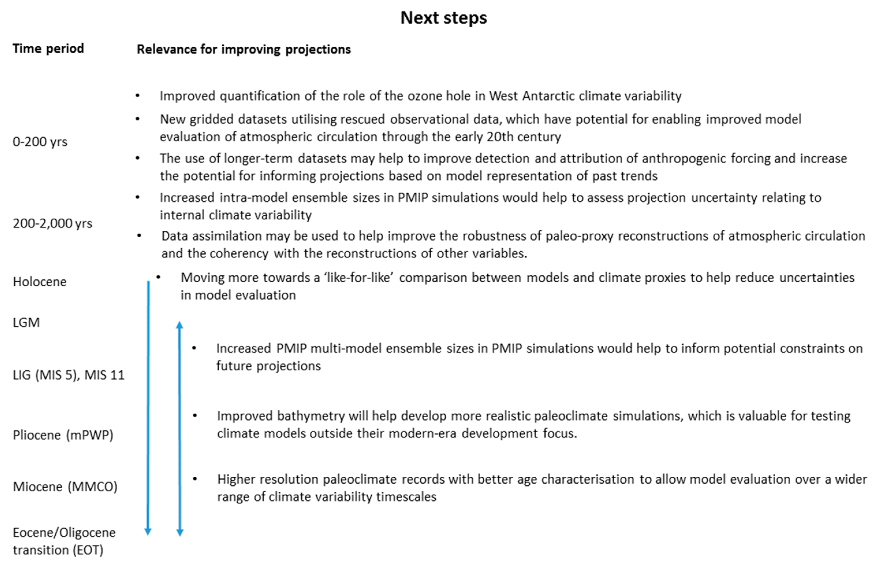
  • Increased PMIP multi-model ensemble sizes in PMIP simulations would help to inform potential constraints on future projections
  • Higher resolution paleoclimate records with better age characterisation to allow model evaluation over a wider range of climate variability timescales
  • Improved bathymetry will help develop more realistic paleoclimate simulations, which is valuable for testing climate models outside their modern-era development focus

4. The Last Two Millennia

This period represents a transition between the present modern instrumental period and the period where climate information comes from a range of different proxy datasets. To help develop datasets for the purpose of climate model evaluation, an important step is to compile regional to continental-scale products that can be directly compared with model outputs. For in-situ weather station observations, large-scale patterns of atmospheric variability can be exploited to develop an Antarctic-wide picture from data gathered/recovered both from Antarctica and further equatorward from land masses along the northern boundary of the Southern Ocean [90]. With regard to ice cores, of the numerous variables measured, many vary with aspects of local, regional, and global climate. The creation of continental-scale ice core climate proxy data networks is complicated by the fact that, in some cases, a single ice core variable (e.g., methane sulfonic acid (MSA)) can represent a distinctly different climate variable depending on where the ice core site is located. In some geographies the year-to-year variability is dominated by onshore-offshore transport, and at others reflects biological production in the sea ice zone. For reasons such as this, great care and objectivity must be exercised when creating a continental-scale ice core climate proxy dataset to be related to a climate variable. As a consequence, this section is arranged into subsections focusing on two groups of variables: (i) temperature, precipitation and surface mass balance and (ii) surface pressure and teleconnections.

4.1. Temperature, Precipitation and Surface Mass Balance

4.1.1. Current State-of-the-Art

There have been significant efforts made to gather Antarctic ice core arrays at a regional scale, e.g., ITASE [91]. Such arrays have been useful for reconstructing past climate over specific regional areas of Antarctica, including West Antarctica [92], the Antarctic Peninsula [93,94], and Wilkes Land [95]. The usefulness of these regional-scale arrays to climate modelers has been enhanced in recent years through efforts to compile multiple regional arrays into continental-scale datasets.
Examples of international efforts to compile and distribute multiple regional-scale ice core datasets include IceReader [http://www.icereader.org/icereader/] and PAGES 2k (e.g., [96,97,98]). This effort should be continued under the auspices of AntClim21 and the PAGES 2k project Climate Variability in Antarctica and Southern Hemisphere in the Past 2000 years (CLIVASH2k). Ultimately, the goal is to compile enough data points (core sites) to create reasonably representative gridded datasets of Antarctica for multiple ice core proxy variables that will be useful for the Antarctic climate modeling community. A key motivation for this approach is that it helps to overcome the issue of spurious (non-climate related) signals in individual records.
A comprehensive evaluation of stable water isotopes from ice cores was compiled by Stenni et al. [98]. Stable water isotopes from the high southern latitudes have long been used as a proxy for past surface temperature. Stenni et al. [98] evaluated 112 ice core records to produce regional and continental-scale temperature reconstructions back to 0 CE. Temperature scaling was based on the δ18O–temperature relationship output from an isotope enabled climate model (ECHAM5-wiso) and by scaling the isotopic normalized anomalies to the variance of the regional reanalysis-estimated temperature. Significant warming trends during the past century were identified in West Antarctica, the Dronning Maud Land coast, and the Antarctic Peninsula.
For surface mass balance (SMB), the PAGES Antarctica2k working group compiled a database of 79 ice core snow accumulation records spanning the last millennium [96]. Snow accumulation is the sum of precipitation, sublimation/solid condensation, runoff/refreeze, and erosion/deposition by the wind determined by annual layer counting of seasonally deposited chemical species. Unlike other ice core proxies, such as stable water isotopes, the snow accumulation is comparable to modelled SMB from regional atmospheric circulation models as for instance RACMO2 or MAR models [99]. To first order, high resolution and quality controlled SMB datasets [100] satisfactorily compare with precipitation minus evaporation (P-E) from global reanalysis products in areas where runoff is small, which is the case for most of the ice sheet. As such, the regional composites compiled in Thomas et al. [96] were compared directly with SMB from output of the RACMO2 atmospheric model [101] to estimate changes in SMB (Gt per year) in seven geographically-distinct regions of Antarctica since 1800 AD. Moreover, the ice core databases have been converted to a gridded reconstruction of annual P−E based on three global atmospheric reanalysis products, specifically the European Centre for Medium-Range Weather Forecasts “Interim” (ERA-Interim), the NASA Modern Era Retrospective Analysis for Research and Applications version 2 (MERRA-2), and the National Centers for Environmental Prediction Climate Forecast System Reanalysis (CFSR) [102].
The ice core snow accumulation records have been used in a number of recent studies to evaluate the performance of climate models, including the regional atmospheric climate model (RACMO2) [103] and the longer reanalysis datasets such as ERA 20C [104]. Another recent study confirms that the observed temporal variability in SMB (from ice cores) is also captured by Global Circulation Models (GCMs) [105].
Relevance for improving projections
  • Improved estimates of natural climate variability, and therefore its potential impact on projected change over the 21st century and beyond

4.1.2. Current Challenges

For Antarctic near-surface air temperature trends there are discrepancies between reconstructions, which indicate limited, non-significant continent-scale temperature trends, and the warming trends simulated by historical (1850–2005) climate simulations [90,106,107]. The Antarctic-wide picture masks contrasting behavior in different regions of Antarctica, such as the significant warming trends in West Antarctica and on the Antarctic Peninsula shown in the regional ice core isotope composites compiled by [98]. Although this provides potentially important information on regional-scale climate processes, significant features such as mountains on spatial scales smaller than a climate model grid box (typically ~100 km for most global climate and earth system models) may make it more challenging to robustly evaluate climate models [81]. However, identifying specific modes of atmospheric variability, such as the changing Southern Annular Mode (SAM) and Pacific South American (PSA) pattern, and focusing on relevant regions and datasets, has the potential to provide a useful approach to model evaluation [108,109]. Last Millennium simulations from the 3rd Paleoclimate Model Intercomparison Project (PMIP3) have also been compared to long-term Antarctic temperature reconstructions. These Last Millennium simulations were conducted as a subset of CMIP5 runs, forced by key drivers of change over this period: volcanic eruptions, vegetation changes, orbital parameters and some changes in greenhouse gas concentrations [110]. These simulations do not exhibit a clear difference from Antarctic temperature reconstructions in terms of multi-decadal variability [109]. However, on shorter decadal timescales the PMIP3 models exhibit larger variability than the reconstructed record. The reasons for this difference are difficult to identify and could include:
  • uncertainty in forcings (e.g., vegetation, volcanic eruptions, solar variability) used to drive the models;
  • misrepresentation or omission of physical processes within the models (e.g., uncertainty in representing anthropogenic aerosol processes and challenges in simulating extreme air-sea interaction conditions at high latitudes);
  • the sparse and uneven availability of proxy data;
  • biases in the reconstructions due to post-deposition effects, non-climatic influences on the records, or the complex relationship between some proxies (in particular δ18O) and climate variables (see for instance [111]).
  • non-stationarity in relationships between variables of interest (such as changing SAM -temperature relationships [112], and PSA - SAM pressure relationships [113] ); or
  • Incorrect assessment and interpretation ice sheet surface mass balance from ice cores, for instance due to omission high precipitation events resulting from maritime air intrusions [114].
Relevance for improving projections:
  • A ‘good’ model could exhibit biases in variability due to uncertainty in the amplitude of natural forcing of variability such as volcanic eruptions
  • Key processes currently omitted or misrepresented in climate models may significantly bias estimates of future climate change impact
  • Non-stationarity in relationships such as the SAM-temperature relationship are an important consideration when comparing models and reconstructions

4.1.3. Next Steps

The physical variables simulated by climate models are often not directly comparable with the biological or environmental variables derived from natural archives (e.g., [115]). For example, in the case of past climatic proxy data, the temporal resolution of natural archives often does not resolve the seasonal cycle. Thus, the traditional data-model comparison is biased by the mis-interpretation of the time averages that specific proxies are related to (from mean annual to mean seasonal). Ice core isotope records are not as simple a proxy for air temperature as previously thought. It is thus required to better understand the detailed processes that are incorporated in oxygen and deuterium isotopes in various types of natural archives globally. This also highlights the need to develop alternative techniques for data-model comparison, including the incorporation of proxy system models [116] and isotopic tracers into climate models. Alternative approaches that can be employed in the interim include the use of pseudo-proxy approaches in comparisons of proxy data and model output, and the careful selection of the most appropriate model variables for comparison.
In the case of past surface temperature, the most commonly used proxy is stable water isotopes. The process of air-mass cooling as moisture is transported to the poles, and the progressive loss of heavy water molecules along the condensation pathway, is well understood [117]. However, the relationship between stable water isotopes in snow and surface temperatures is also dependent on a number of other factors and may vary spatially and temporally. For example, changes in evaporation conditions and moisture origin, shifts in atmospheric transport pathways, and precipitation seasonality will all influence the δ18O - temperature conversion [97]. A recent study highlighted the degree to which Antarctic precipitation is dominated by extreme precipitation events, especially in regions such as West Antarctica [114], which will undoubtedly have a strong influence on the δ18O record preserved in ice cores. Thus, it is preferable to compare stable isotope records from ice cores with stable water isotope enabled climate models, such as ECHAM-wiso, following the approach of [98,118]. However, a recent study using GCM simulations advocated the use of SMB as a proxy for past surface temperature over the past 2000 years ([105], this issue). They demonstrated a stronger link between surface temperature and SMB in model simulations than that of δ18O and surface temperature at a regional scale.
Limitations still exist in properly modeling the surface energy balance, and hence heating and/or melt rate of Antarctic snow and ice, saltation of snow, and sublimation and albedo in ESMs [99,119,120], as well as the polar ocean and sea ice [87] and this is especially difficult due the complexities of conducting accurate field observations, especially across large geographic domains. Additionally, within Antarctica, little effort has been made to robustly organize and standardize physical snow observations, which is important for closing the surface energy balance, as well as for interpreting ice core records. Furthermore, the radiative forcing of impurities in the cryosphere, such as black carbon, are currently reported with 90% uncertainty bounds [121] and there is a need for further observations to refine models of snow physical and optical properties (e.g., [122,123]) and of their impact on absorption and reflectance [124]. Future work should include efforts to address these limitations in representing the surface energy balance with fieldwork being particularly important for providing the necessary data to help refine numerical models.
Because the computational costs of paleoclimate simulations remain prohibitive, only a small number of simulations are typically conducted, which is a key limitation since there is a need for ensembles of multiple simulations to be conducted using each model in order to quantify and assess the uncertainty arising from unforced internal climate variability. An exception to this, which demonstrates the potential for progress in this area, is the CESM1 Last Millennium Ensemble [125].
Relevance for Improving Projections:
  • Moving more towards a ‘like-for-like’ comparison between models and climate proxies will likely help reduce uncertainties in model evaluation
  • Increased intra-model ensemble sizes in PMIP simulations would help to assess projection uncertainty relating to internal climate variability

4.2. Surface Pressure and Teleconnections

4.2.1. Current State-of-the-Art

A number of modern re-analysis systems have been used to develop products that go back before the modern observational and satellite eras (ERA-20C, CERA20C, 20CR). In regions with a sufficient number of long-term weather stations, such as over Europe, they have reasonable reliability even in the early 20th century. However, in data-sparse regions, such as the high-latitude SH, reliability before the mid-20th century is poor (e.g., [126,127]). Rescue of historical observations as undertaken by projects such as Atmospheric Circulation Reconstructions over the Earth (ACRE) can contribute towards reducing these errors.
A number of studies have used the teleconnections between pressure at mid and high latitudes in the SH to produce reconstructions of atmospheric circulation and pressure back to the early 20th century. Jones, et al. [128] produced seasonal reconstructions of the SAM using mid latitude sea-level pressure (SLP) records; using these reconstructions Fogt, et al. [129] found that global climate models underestimate natural variability in the SAM in the 1930s and 1960s. SLP records from mid-latitude stations were also used to reconstruct surface pressure at Antarctic stations back to 1905 [130]. Reconstruction skill was found to be better in austral summer than in winter. These reconstructions were extended to produce a gridded surface pressure reconstruction poleward of 60°S in Austral summer, and forcing mechanisms of the reconstructed pressure changes were explored through comparison with simulations with the Community Atmospheric Model, version 5 (CAM5) [131]. These reconstructions offer the possibility of both further use for model evaluation, as well as for comparison with, and calibration of, proxy records.
Various proxy networks and methodologies have been used for reconstructing SAM during the last millennium. These include annual and summer reconstructions based on temperature-sensitive temperature proxies from across the SH [15], annual average reconstructions using SAM-temperature correlation patterns across the Antarctica-S. America sector [132] and summer reconstructions derived from S. America or New Zealand tree ring records [133]. The reconstructions show differences in scaling but all suggest that the most negative SAM conditions of the last millennium occurred about 1400 CE, and that SAM is characterized by large multi-decadal variability.
Relevance for improving projections:
  • Multi-proxy circulation reconstructions are best suited for evaluation of model-simulated hemispheric-scale SAM variability
  • SAM reconstructions (both proxy and instrumental) are most consistent in summer, which is therefore most relevant to projections in this season

4.2.2. Current Challenges

Current key challenges in developing reconstructions of past atmospheric circulation variability and trends are (i) improving the reliability for non-summer months (and the annual mean), (ii) developing more reliable regional (non-annular) reconstructions and (iii) extracting more detail about whether variability and trends in the SAM is are related more to shifting or strengthening/weakening of the Southern Ocean westerlies or indeed changes in non-annular features such as the ASL (e.g., [134]). Reconstructions of the SAM show large multi-decadal variability, but robustness of the reconstructions at this time-scale is difficult to assess because of the potential non-stationarity of the teleconnections [113]. Models generally display less variability at multi-decadal timescales than the reconstructions [109] and the mechanisms potentially responsible for such low frequency changes need a deeper investigation. Reconstructing circulation trends in greater detail is important since, for example, shifting and/or strengthening of the westerly jet have different drivers and different impacts on, for example, sea ice [5,135,136].
Relevance for improving projections:
  • Current reconstructions limit the scope for evaluation of non-annular circulation patterns and/or jet stream shifting or strengthening associated with SAM variability
  • There is a need to better understand model-reconstruction differences in multi-decadal variability in order to increase confidence in using such information to inform projections

4.2.3. Next Steps

Early 20th-century observations retrieved through data rescue projects have the potential to improve historical reanalyses, but also to be used to evaluate these long-term reanalyses and help to develop specific southern mid-high latitude gridded circulation reconstructions. Rescue and use of observations located in the high latitude SH is particularly important, as existing reconstructions are based on mid-latitude data. There is also the potential to use such observations, or the resulting reconstructions, for comparison with proxy records (e.g., ice cores), and for model evaluation for non-Antarctic regions [137]. Longer-term pre-modern-observational-era observations have been little used for model evaluation so far. This may partly be because it is only relatively recently that large-scale data rescue and digitization efforts have been undertaken (e.g., through ACRE, and citizen science in initiatives such as Old Weather). The fact that it may be unclear to modelers that such data are taken using very similar methods/instruments to today, so are more trustworthy than may be thought, may also be a reason for lack of use. Gridded datasets would make these observations suitable for use by climate modelers, particularly as they can provide monthly and seasonal information, and are direct measurements of the variables of interest (SST, SLP, wind, and air temperature).
The available reconstructions of circulation changes covering several centuries are generally independent of reconstructions for other variables, but atmospheric circulation variability is intrinsically coupled to changes in surface temperature, precipitation and surface mass balance. Taking advantage of the covariance between those variables offers the possibility to reduce the uncertainties on the reconstructions for each of them individually and to provide consistent reconstructions that allow a better interpretation of the potential origin of the changes. This is the basis of the data assimilation approach, leading to the long-term reanalyses that have been carried out very recently [105,113,138]. A systematic evaluation of existing reanalyses offers many opportunities, but new reanalyses are needed that take account of the proxies in the high latitudes of the Southern Ocean, in particular those directly related to circulation changes.
Relevance for improving projections:
  • New gridded datasets utilising rescued data would have potential for improved model evaluation of atmospheric circulation through the early 20th century
  • Improving the robustness of paleo-proxy reconstructions of atmospheric circulation and the coherency with the reconstructions of other variables (e.g., through data assimilation) would help to improve the evaluation of climate variability in models and its role in projections

5. The Emergence of Anthropogenic Climate Signals

Looking back at past climate variability and change can potentially help to determine the extent to which humans are responsible for recent and current observed trends in Antarctic climate. This is relevant to estimating future climate change since the amplitude of detectable anthropogenic signals in historical data is potentially useful for informing such estimates (e.g., [139]). In the climate science community quantitative ‘detection and attribution’ (D&A) methods are widely used to establish the human contribution to recent/current trends. D&A refers to the two stage processes of first detecting a statistically significant signal that cannot be explained by internal climate variability followed by the second attribution stage of identifying the cause (or causes). All known potentially important forcings, both natural and anthropogenic, should ideally be considered.
The climate system over Antarctica exhibits the largest internal variability on the planet (e.g., [140,141]), therefore externally-driven anthropogenic climate change signals can emerge later relative to lower latitudes. However, where anthropogenic signals can be identified in observations, then there is potential for constraining estimates of future change based on the extent to which climate models over- or under-estimate the strength of a given signal [139]. This can help in regions of large internal climate variability such as around Antarctica. Two defining questions for this section are: (i) In what variables in the modern era have effects from anthropogenic forcing been detected? And (ii) how can longer-term datasets help to improve Antarctic D&A analyses? To answer the first question, a comprehensive suite of model simulations, robust and appropriate statistical methods, and long-term reliable observations are all required. The latter point clearly links to the second question, whereby extensions to the modern observational era are of potential benefit in the detection and attribution of Antarctic climate and environmental change.
In this section we first outline the different ways in which anthropogenic signals have been detected across a range of variables. The role, or potential role, of long-term datasets in improving D&A for Antarctica is then highlighted along with relevance to improving climate change projections to 2100.

5.1. Anthropogenic Signals in Antarctic Variables

For many parameters the emergence of a detectable anthropogenic signal in Antarctica may not occur until the second half of the 21st century [142,143]. However, careful analysis of a range of variables has revealed a detectable human influence in many aspects of Antarctic and Southern Ocean climate. A number of these studies involve the use of a powerful methodology to consider differences in the spatial patterns of climate response to different forcings, known as ‘optimal fingerprinting’ [144,145].

5.1.1. Temperature

In the modern instrumental era an anthropogenic signal has been detected in observed spatial patterns of surface temperature change in terrestrial Antarctic observation stations [146]. Another variable showing success is Southern Ocean subsurface temperatures (warming), for which a response has been detected and recently attributed to GHG and stratospheric ozone change from the 1950s to now [145].
The reconstruction of Stenni et al. [98] complements Gillett et al. [146] by providing a longer-term perspective on different regions of Antarctica. They found that the Antarctic Peninsula is the only region in which the most recent century-scale trend is unusual in the context of natural variability over the last 2000 years. An ice core melt history from the Antarctic Peninsula also identifies the unusual acceleration in surface melting associated with regional warming, and validates expectations of a non-linear threshold response of surface melt to temperature change [147].

5.1.2. SMB

Regional composites [96] and spatial reconstructions [102] highlight the large regional differences in SMB across Antarctica. The Antarctic Peninsula has experienced dramatic increases in snow accumulation during the 20th century, related to changes in large-scale modes of atmospheric variability (especially SAM), tropical teleconnections and local sea ice conditions. This region also exhibits the largest multi-decadal variability over the past two centuries.
Simulations covering the past millennium display an increase in SMB over the past century similar to the one of [96] for the whole continent but generally fail in reproducing the regional differences. This may be due the large internal variability observed and simulated at regional scale. Models also simulate a strong link between large scale temperature and SMB variability over the past centuries, as derived from modern observations [105].
Although the large internal variability makes detection of a statistically-significant signal in SMB difficult, modeling suggests that stratospheric ozone depletion acting alone would drive an increase in Antarctic SMB [148]. However, sea ice extent appears to be an important factor in Antarctic precipitation trends [149] and the response of sea ice to stratospheric ozone depletion in models has been found to be highly model dependent [150]. Therefore, it will be important to evaluate the link between ozone depletion (and indeed other forcings) and SMB across a wider range of Earth System Models. Nevertheless, the anthropogenic impact on Antarctic surface mass balance will be likely masked by natural variability until mid-century [151].

5.1.3. Atmospheric Circulation

Some success has been documented in detecting and attributing change for a number of Antarctic variables. For sea-level pressure (SLP), it has been shown that decreases and associated geostrophic wind increases can be attributed to greenhouse gas, sulfate aerosol, stratospheric ozone, volcanic aerosol and solar forcing [10,152,153]. It should be noted that since these papers were published, reliable reconstructions of Antarctic surface pressure now exist back to 1905 [130] although the reconstruction does not extend over the surrounding oceans.
Extending beyond regional circulation to hemispheric-scale trends in the SAM, robust and consistent changes are observed across observations, models and reconstructions since the mid-20th Century [15,154]. These exceed model-generated internal variability and with the most prominent trends in summer attributed to stratospheric ozone depletion (e.g., [155,156]).

5.1.4. Sea Ice

Attempts to determine the Southern Ocean sea ice response to anthropogenic forcing have been hampered by the relatively short modern satellite record and the weak signal compared to simulated internal variability. There is also an apparent contrast between observed slight increases (a spatially-heterogeneous overall increase, most intense in the austral autumn) in Antarctic SIE and overall declines simulated by the majority of climate models in response to anthropogenic forcing [157,158,159,160]. Much of the observed trend in sea ice extent adjacent to West Antarctica is thought to be due to wind changes related to tropical Pacific variability [161,162], compounding the issue of identifying the true physical response to anthropogenic forcings. Ocean-sea ice feedbacks may be important for explaining the observed trends [163], and there is evidence that inadequate representation of the subsurface ocean could be a major model deficiency [164,165]. The lack of year-round ocean observations in the sea ice zone is a challenge for validating these model processes.
A number of approaches have been used to overcome these challenges. Proxy reconstructions have been used to extend the sea ice record throughout the 20th century, but an anthropogenic forcing response is still not formally detectable. Reliable proxies are not available for the region of greatest change (the western Ross Sea) or the seasons of greatest change (summer and autumn) [166]. A number of ice core proxies exist and the most widely used is methane sulfonic acid (MSA), which gives information about winter maximum sea ice extent [147,167]. MSA-based reconstructions have revealed a 20th century sea ice decline in the Bellingshausen Sea [168], while sea ice has increased in the Amundsen-Ross Sea over the same period [169]. Although these contrasting trends suggest a strengthening of the dipole between the Bellingshausen and the Ross Sea, comparisons with early satellite records suggest that proxy records from this region may not be reliable [166]. The meridional circulations in West Antarctica that drive much of the observed trends and variability are prone to east-west shifts, which means that the source location of proxy chemicals also shift, leading to a confounding factor in reconstructing local sea ice changes; combining proxies from multiple sites may allow a reconstruction of the evolution of these zonal shifts. Seasonally, the most reliable proxy for inter-annual sea ice variability (MSA) is a proxy for winter sea ice extent and hence an alternative proxy would be required to reconstruct warm season sea ice variability.
A potentially useful approach to characterize sea ice trends is to evaluate trends in factors that may drive these trends. An example where the current generation of climate models shows promise, but also offers large areas for improvement, is in attributing the role of stratospheric ozone depletion on recent historic regional Antarctic sea ice trends. Ozone depletion has been demonstrated to be the largest driver of SH atmospheric circulation changes in the twentieth century [13,14], so the expectation is that its effect on Antarctic sea ice should be detectable. The largest regional trends in sea ice are located to the east and west of the ASL [8,9]. This regional low pressure feature has been offered as a potential explanation of the regional pattern of SIE trends [170] although the relationship between the ASL and sea ice is complex [171]. Despite the large internal variability in this region, stratospheric ozone depletion has been shown to cause a deepening of the ASL in austral summer [10]. Models are able to capture the inter-annual relationship between the ASL and autumn sea ice and yet the observed sea ice trends nearly diametrically oppose what the models project in response to stratospheric ozone depletion [172]. It is possible that internal variability overwhelms the sea ice response to the ozone hole [157,173,174] but another option is that climate models are lacking in their representation of ocean-atmosphere-sea ice coupling. Improvements in understanding of the climate variability in West Antarctica could be key for placing the response to stratospheric ozone depletion in appropriate context.

5.2. Incorporating Longer-Term Datasets in Antarctic D&A

The survey of different variables in the previous section shows that longer-term datasets are key to setting recent trends in a longer-term context. However, there are challenges in terms of developing proxy and station-based reconstructions with a small enough uncertainty for effective use in formal D&A methods, particularly in relation to sea ice where reconstructions require indirect relationships linking SIE to the proxy signal. If these challenges can be overcome, the most direct link to projections is the ability to quantify the degree to which a given climate model may over- or under-estimate historical responses to climate forcings (or a specific forcing). This can help to inform whether a given model may over- or under-estimate projected future change [139]. Important considerations are a changing mix of forcings, as stratospheric ozone begins to recover, and a range of response timescales (e.g., [175]). A key caveat is also that historical model trend biases may not be constant into the future.
There are a number of possibilities going forward with regard to better integrating long-term datasets in Antarctic D&A studies. (i) The use of better methods to link large-scale and small-scale processes. For example, using regional high-resolution atmospheric numerical models (including water isotopes in regional circulation models) to assess regional signals in particular for interpolation of sparse data/signals. (ii) Atmospheric regional downscaling may prove especially useful in assessing how spatially representative local (ice/sediment core) signals are [98], especially in regions of strong climate gradients (e.g., the Antarctic Peninsula or West Antarctica). (iii) Better quantification of the contributions from fast and slow components of the Antarctic climate system (ocean intermediate and deep circulation, ice sheet dynamics and related glacio-isostatic adjustment) since there is a need to determine the extent to which observed temperature trends, and other variables such as ice-sheet velocities, calving rates, basal melt rates, are the result of anthropogenic climate change rather than long-term climate evolution inherited from the last deglaciation.
Relevance for improving projections:
  • Anthropogenic signals are still not detectable in sea ice and therefore it is difficult to evaluate robustness of projections
  • Improved quantification of the role of the ozone hole in West Antarctic climate variability is a key foundation for improving projections of broader environmental change
  • Improved detection and attribution scaling would provide a basis for scaling climate model projections

6. Conclusions

This paper presents an analysis of how long-term observational and paleoclimate data may help to improve Antarctic climate model projections for the 21st century. A key novelty of this study is the wide range of timescales, from instrumental reconstructions of the early 20th century back through different climate regimes to the EOT, 34 Ma. The rationale for this is to synthesize and compare the wide range of different ways in which longer-term datasets may be of value to climate model evaluation.
Trust in future projections of Antarctic climate relies to a large extent on whether climate models are able to reproduce past observable behavior of the climate system. However, this alone does not guarantee a realistic response to future forcing, since it is also important to include processes known to be, or likely to become, important for the aspect of climate being evaluated.
Figure 2, Figure 3 and Figure 4 show schematics that summarize the main points as presented in the text, which focus on relevance for improving projections in the context of state-of-the-art (Figure 2), current challenges (Figure 3) and next steps in making improvements (Figure 4). Across the different time periods considered, key ways in which long-term climate reconstructions may help improve projections are:
  • Reconstructions of past conditions are being used to identify climate model variants that best match past conditions and therefore provide the potential to narrow uncertainty in projections; wide participation in multi-model paleo-focused MIPs such as CMIP6-PMIP is encouraged.
  • Improved paleo bathymetric data has the potential to better constrain past reconstructions and future simulations of freshwater fluxes from ice sheet melting, oceanic heat exchange between regional polar oceans and the open ocean, and impacts of freshwater release on the Southern Ocean.
  • Recent progress in compiling long term extended instrumental and paleo-proxy records are providing improved information on decadal-to-centennial variability of the Antarctic climate system that may help to provide insight into the realism of the pronounced variability generated internally within the latest earth system models. There are both opportunities and challenges in assessing how drivers of variability (such as ENSO) influence climate indices such as the SAM and climatic conditions over Antarctica.
  • To date formal D&A Antarctic studies have focused on the modern instrumental era, but there is potential to incorporate longer-term datasets and to help narrow the uncertainty range on detected signals.
  • An overall recommendation that is not specific to the time periods or processes considered in this paper is for communities working on long-term Antarctic climate reconstructions to produce datasets for use in routine climate model evaluation. In this way, the paleoclimate information could be a more prominent part of the standard model development and testing cycle and feed directly into improving and developing the next generation of climate and earth-system models. A prominent example of a repository for observational data for use in model evaluation is the Obs4MIPs project (https://esgf-node.llnl.gov/projects/obs4mips/). Many aspects of the gridded reconstructions of Antarctic climate that have been generated as part of synthesis projects, such as PAGES Antarctica2k, could be adapted to conform to the formatting and uncertainty estimation requirements.
Looking to the future, our overall conclusion is that closer integration between the climate reconstruction and climate modelling communities would be of great benefit for improving the reliability of projections of future Antarctic climate change. This should be achieved through a combination of: (i) extending the range of climate model outputs to better match key climate proxies, (ii) feeding long-term reconstruction datasets into community standard climate modelling metrics, (iii) encouraging participation in PMIP or other project simulations as a high priority for model centers and (iv) regular workshops and meetings to encourage collaboration and sharing of tools and data across the modern and paleo climate communities. This approach is encouraged by SCAR, whose future scientific plan under development will follow an integrated research approach across the existing SCAR working groups to encourage multi-disciplinary research of past to future polar sciences and provide more reliable projections of Antarctic climate and ice sheet contribution to global mean sea level rise.

Author Contributions

Conceptualization, T.J.B., F.C., N.J.A., N.A.N.B., D.A.D., M.E., V.F., C.J.F., J.C.F., I.G., H.G., W.H., J.M.J., E.D.K., A.L.K., M.N.R., J.R., L.S., E.R.T., M.R.B., I.W.; writing—original draft preparation, T.J.B., F.C., N.J.A., N.A.N.B., D.A.D., M.E., V.F., C.J.F., J.C.F., I.G., H.G., W.H., J.M.J., E.D.K., A.L.K., S.J.P., M.N.R., J.R., L.S., E.R.T., M.R.B., I.W.; writing—review and editing, T.J.B., F.C., N.J.A., D.A.D., V.F., C.J.F., W.H., J.M.J., S.J.P., E.R.T., M.R.B., I.W.; visualization, T.J.B., F.C.

Funding

The Antarctic Climate Change in the 21st Century (AntClim21) Scientific Research Programme of the Scientific Committee on Antarctic Research are thanked for supporting the international scientific workshop at which the writing of this manuscript was initiated. This is a contribution to the PAGES 2k Network (through the CLIVASH 2k project). NJA acknowledges support by the Australian Research Council through a Future Fellowship (FT160100029) and the Centre of Excellence for Climate Extremes (CE170100023). SJP was supported under the Australian Research Council’s Special Research Initiative for the Antarctic Gateway Partnership (Project ID SR140300001). JMJ acknowledges support from the Leverhulme Trust through a Research Fellowship (RF-2018-183). FC acknowledges support from the PNRA national Italian projects PNRA16_00016, “WHISPERS” and project PNRA_00002, “ANTIPODE”. TJB, LS, and ERT were supported by the Natural Environment Research Council (NERC) as part of the British Antarctic Survey Polar Science for Planet Earth Programme. TJB additionally acknowledges support for this work as a contribution to the NERC grant NE/N01829X/1. IW thanks FAPESP 2015/50686-1, Coordenação de Aperfeiçoamento de Pessoal de Nível Superior - Brasil (CAPES) Finance Code 001 and CNPq 300970/2018-8, CNPq INCT Criosfera 704222/2009.

Acknowledgments

Two anonymous reviewers are thanked for their insightful and constructive suggestions, which helped to significantly improve the manuscript.

Conflicts of Interest

The authors declare no conflicts of interest.

References

  1. Flato, G.; Marotzke, J.; Abiodun, B.; Braconnot, P.; Chou, S.C.; Collins, W.; Cox, P.; Driouech, F.; Emori, S.; Eyring, V.; et al. Evaluation of Climate Models; Cambridge University Press: Cambridge, UK; New York, NY, USA, 2013. [Google Scholar]
  2. Nowicki, S.; Seroussi, H. Projections of Future Sea Level Contributions from the Greenland and Antarctic Ice Sheets Challenges beyond Dynamical Ice Sheet Modeling. Oceanography 2018, 31, 109–117. [Google Scholar] [CrossRef]
  3. Collins, M.; Knutti, R.; Arblaster, J.; Dufresne, J.-L.; Fichefet, T.; Friedlingstein, P.; Gao, X.; Gutowski, W.J.; Johns, T.; Krinner, G.; et al. Long-term Climate Change: Projections, Commitments and Irreversibility. In Climate Change 2013: The Physical Science Basis. Contribution of Working Group I to the Fifth Assessment Report of the Intergovernmental Panel on Climate Change; Cambridge University Press: Cambridge, UK, 2013. [Google Scholar]
  4. Bracegirdle, T.J.; Hyder, P.; Holmes, C.R. CMIP5 diversity in southern westerly jet projections related to historical sea ice area; strong link to strengthening and weak link to shift. J. Clim. 2018, 31, 195–211. [Google Scholar] [CrossRef]
  5. Chavaillaz, Y.; Codron, F.; Kageyama, M. Southern westerlies in LGM and future (RCP4.5) climates. Clim. Past 2013, 9, 517–524. [Google Scholar] [CrossRef] [Green Version]
  6. Krinner, G.; Largeron, C.; Menegoz, M.; Agosta, C.; Brutel-Vuilmet, C. Oceanic Forcing of Antarctic Climate Change: A Study Using a Stretched-Grid Atmospheric General Circulation Model. J. Clim. 2014, 27, 5786–5800. [Google Scholar] [CrossRef] [Green Version]
  7. Limpasuvan, V.; Hartmann, D.L. Eddies and the annular modes of climate variability. Geophys. Res. Lett. 1999, 26, 3133–3136. [Google Scholar] [CrossRef] [Green Version]
  8. Turner, J.; Phillips, T.; Hosking, J.S.; Marshall, G.J.; Orr, A. The Amundsen Sea low. Int. J. Climatol. 2013, 33, 1818–1829. [Google Scholar] [CrossRef]
  9. Turner, J.; Comiso, J.C.; Marshall, G.J.; Lachlan-Cope, T.A.; Bracegirdle, T.J.; Maksym, T.; Meredith, M.P.; Wang, Z.; Orr, A. Non-annular atmospheric circulation change induced by stratospheric ozone depletion and its role in the recent increase of Antarctic sea ice extent. Geophys. Res. Lett. 2009, 36, L08502. [Google Scholar] [CrossRef]
  10. England, M.R.; Polvani, L.M.; Smith, K.L.; Landrum, L.; Holland, M.M. Robust response of the Amundsen Sea Low to stratospheric ozone depletion. Geophys. Res. Lett. 2016, 43, 8207–8213. [Google Scholar] [CrossRef]
  11. Karoly, D.J. Southern Hemisphere circulation features associated with El Niño-Southern Oscillation events. J. Clim. 1989, 2, 1239–1252. [Google Scholar] [CrossRef]
  12. Stevenson, S.; Fox-Kemper, B.; Jochum, M.; Neale, R.; Deser, C.; Meehl, G. Will There Be a Significant Change to El Nino in the Twenty-First Century? J. Clim. 2012, 25, 2129–2145. [Google Scholar] [CrossRef]
  13. Arblaster, J.M.; Meehl, G.A. Contributions of external forcings to southern annular mode trends. J. Clim. 2006, 19, 2896–2905. [Google Scholar] [CrossRef]
  14. Polvani, L.M.; Waugh, D.W.; Correa, G.J.P.; Son, S.-W. Stratospheric Ozone Depletion: The Main Driver of Twentieth-Century Atmospheric Circulation Changes in the Southern Hemisphere. J. Clim. 2011, 24, 795–812. [Google Scholar] [CrossRef]
  15. Datwyler, C.; Neukom, R.; Abram, N.J.; Gallant, A.J.E.; Grosjean, M.; Jacques-Coper, M.; Karoly, D.J.; Villalba, R. Teleconnection stationarity, variability and trends of the Southern Annular Mode (SAM) during the last millennium. Clim. Dyn. 2018, 51, 2321–2339. [Google Scholar] [CrossRef]
  16. Gillett, N.P.; Fyfe, J.C. Annular mode changes in the CMIP5 simulations. Geophys. Res. Lett. 2013, 40, 1189–1193. [Google Scholar] [CrossRef]
  17. Bracegirdle, T.J.; Stephenson, D.B.; Turner, J.; Phillips, T. The importance of sea ice area biases in 21st century multimodel projections of Antarctic temperature and precipitation. Geophys. Res. Lett. 2015, 42. [Google Scholar] [CrossRef]
  18. Holloway, M.D.; Sime, L.C.; Singarayer, J.S.; Tindall, J.C.; Bunch, P.; Valdes, P.J. Antarctic last interglacial isotope peak in response to sea ice retreat not ice-sheet collapse. Nat. Commun. 2016, 7. [Google Scholar] [CrossRef] [PubMed]
  19. Thompson, A.F.; Stewart, A.L.; Spence, P.; Heywood, K.J. The Antarctic Slope Current in a Changing Climate. Rev. Geophys. 2018, 56, 741–770. [Google Scholar] [CrossRef]
  20. Braconnot, P.; Harrison, S.P.; Kageyama, M.; Bartlein, P.J.; Masson-Delmotte, V.; Abe-Ouchi, A.; Otto-Bliesner, B.; Zhao, Y. Evaluation of climate models using palaeoclimatic data. Nat. Clim. Chang. 2012, 2, 417–424. [Google Scholar] [CrossRef]
  21. Lear, C.H.; Elderfield, H.; Wilson, P.A. Cenozoic deep-sea temperatures and global ice volumes from Mg/Ca in benthic foraminiferal calcite. Science 2000, 287, 269–272. [Google Scholar] [CrossRef]
  22. Fischer, H.; Meissner, K.J.; Mix, A.C.; Abram, N.J.; Austermann, J.; Brovkin, V.; Capron, E.; Colombaroli, D.; Daniau, A.L.; Dyez, K.A.; et al. Palaeoclimate constraints on the impact of 2 degrees C anthropogenic warming and beyond. Nat. Geosci. 2018, 11, 474–485. [Google Scholar] [CrossRef]
  23. Eyring, V.; Bony, S.; Meehl, G.A.; Senior, C.A.; Stevens, B.; Stouffer, R.J.; Taylor, K.E. Overview of the Coupled Model Intercomparison Project Phase 6 (CMIP6) experimental design and organization. Geosci. Model Dev. 2016, 9, 1937–1958. [Google Scholar] [CrossRef] [Green Version]
  24. Otto-Bliesner, B.L.; Braconnot, P.; Harrison, S.P.; Lunt, D.J.; Abe-Ouchi, A.; Albani, S.; Bartlein, P.J.; Capron, E.; Carlson, A.E.; Dutton, A.; et al. The PMIP4 contribution to CMIP6-Part 2: Two interglacials, scientific objective and experimental design for Holocene and Last Interglacial simulations. Geosci. Model Dev. 2017, 10, 3979–4003. [Google Scholar] [CrossRef]
  25. Kageyama, M.; Albani, S.; Braconnot, P.; Harrison, S.P.; Hopcroft, P.O.; Ivanovic, R.F.; Lambert, F.; Marti, O.; Peltier, W.R.; Peterschmitt, J.-Y.; et al. The PMIP4 contribution to CMIP6-Part 4: Scientific objectives and experimental design of the PMIP4-CMIP6 Last Glacial Maximum experiments and PMIP4 sensitivity experiments. Geosci. Model Dev. 2017, 10, 4035–4055. [Google Scholar] [CrossRef]
  26. Lunt, D.J.; Abe-Ouchi, A.; Bakker, P.; Berger, A.; Braconnot, P.; Charbit, S.; Fischer, N.; Herold, N.; Jungclaus, J.H.; Khon, V.C.; et al. A multi-model assessment of last interglacial temperatures. Clim. Past 2013, 9, 699–717. [Google Scholar] [CrossRef] [Green Version]
  27. Haywood, A.M.; Dowsett, H.J.; Dolan, A.M.; Rowley, D.; Abe-Ouchi, A.; Otto-Bliesner, B.; Chandler, M.A.; Hunter, S.J.; Lunt, D.J.; Pound, M.; et al. The Pliocene Model Intercomparison Project (PlioMIP) Phase 2: Scientific objectives and experimental design. Clim. Past 2016, 12, 663–675. [Google Scholar] [CrossRef]
  28. de Boer, B.; Dolan, A.M.; Bernales, J.; Gasson, E.; Goelzer, H.; Golledge, N.R.; Sutter, J.; Huybrechts, P.; Lohmann, G.; Rogozhina, I.; et al. Simulating the Antarctic ice sheet in the late-Pliocene warm period: PLISMIP-ANT, an ice-sheet model intercomparison project. Cryosphere 2015, 9, 881–903. [Google Scholar] [CrossRef] [Green Version]
  29. Lunt, D.J.; Huber, M.; Anagnostou, E.; Baatsen, M.L.J.; Caballero, R.; DeConto, R.; Dijkstra, H.A.; Donnadieu, Y.; Evans, D.; Feng, R.; et al. The DeepMIP contribution to PMIP4: Experimental design for model simulations of the EECO, PETM, and pre-PETM (version 1.0). Geosci. Model Dev. 2017, 10, 889–901. [Google Scholar] [CrossRef]
  30. Waelbroeck, C.; Paul, A.; Kucera, M.; Rosell-Mele, A.; Weinelt, M.; Schneider, R.; Mix, A.C.; Abelmann, A.; Armand, L.; Bard, E.; et al. Constraints on the magnitude and patterns of ocean cooling at the Last Glacial Maximum. Nat. Geosci. 2009, 2, 127–132. [Google Scholar] [CrossRef]
  31. Turney, C.S.M.; Jones, R.T. Does the Agulhas Current amplify global temperatures during super-interglacials? J. Quat. Sci. 2010, 25, 839–843. [Google Scholar] [CrossRef]
  32. Capron, E.; Govin, A.; Stone, E.J.; Masson-Delmotte, V.; Mulitza, S.; Otto-Bliesner, B.; Rasmussen, T.L.; Sime, L.C.; Waelbroeck, C.; Wolff, E.W. Temporal and spatial structure of multi-millennial temperature changes at high latitudes during the Last Interglacial. Quat. Sci. Rev. 2014, 103, 116–133. [Google Scholar] [CrossRef] [Green Version]
  33. Dowsett, H.; Barron, J.; Poore, R. Middle Pliocene sea surface temperatures: A global reconstruction. Mar. Micropaleontol. 1996, 27, 13–25. [Google Scholar] [CrossRef]
  34. Dutton, A.; Carlson, A.E.; Long, A.J.; Milne, G.A.; Clark, P.U.; DeConto, R.; Horton, B.P.; Rahmstorf, S.; Raymo, M.E. Sea-level rise due to polar ice-sheet mass loss during past warm periods. Science 2015, 349. [Google Scholar] [CrossRef] [PubMed]
  35. Laskar, J.; Gastineau, M.; Joutel, F.; Levrard, B.; Robutel, P. A New Astronomical Solution for the Long Term Evolution of the Insolation Quantities of Mars. In Proceedings of the 35th Lunar and Planetary Science Conference, League City, TX, USA, 15–19 March 2004. [Google Scholar]
  36. Luthi, D.; Le Floch, M.; Bereiter, B.; Blunier, T.; Barnola, J.M.; Siegenthaler, U.; Raynaud, D.; Jouzel, J.; Fischer, H.; Kawamura, K.; et al. High-resolution carbon dioxide concentration record 650,000-800,000 years before present. Nature 2008, 453, 379–382. [Google Scholar] [CrossRef] [PubMed]
  37. Pagani, M.; Liu, Z.H.; LaRiviere, J.; Ravelo, A.C. High Earth-system climate sensitivity determined from Pliocene carbon dioxide concentrations. Nat. Geosci. 2010, 3, 27–30. [Google Scholar] [CrossRef]
  38. Stoll, H.M.; Guitian, J.; Hernandez-Almeida, I.; Mejia, L.M.; Phelps, S.; Polissar, P.; Rosenthal, Y.; Zhang, H.R.; Ziveri, P. Upregulation of phytoplankton carbon concentrating mechanisms during low CO2 glacial periods and implications for the phytoplankton pCO(2) proxy. Quat. Sci. Rev. 2019, 208, 1–20. [Google Scholar] [CrossRef]
  39. Beerling, D.J.; Royer, D.L. Convergent Cenozoic CO2 history. Nat. Geosci. 2011, 4, 418–420. [Google Scholar] [CrossRef]
  40. Vacchi, M.; Marriner, N.; Morhange, C.; Spada, G.; Fontana, A.; Rovere, A. Multiproxy assessment of Holocene relative sea-level changes in the western Mediterranean: Sea-level variability and improvements in the definition of the isostatic signal. Earth-Sci. Rev. 2016, 155, 172–197. [Google Scholar] [CrossRef] [Green Version]
  41. Miller, K.G.; Kominz, M.A.; Browning, J.V.; Wright, J.D.; Mountain, G.S.; Katz, M.E.; Sugarman, P.J.; Cramer, B.S.; Christie-Blick, N.; Pekar, S.F. The phanerozoic record of global sea-level change. Science 2005, 310, 1293–1298. [Google Scholar] [CrossRef]
  42. Pusz, A.E.; Thunell, R.C.; Miller, K.G. Deep water temperature, carbonate ion, and ice volume changes across the Eocene-Oligocene climate transition. Paleoceanography 2011, 26. [Google Scholar] [CrossRef] [Green Version]
  43. Kingslake, J.; Scherer, R.P.; Albrecht, T.; Coenen, J.; Powell, R.D.; Reese, R.; Stansell, N.D.; Tulaczyk, S.; Wearing, M.G.; Whitehouse, P.L. Extensive retreat and re-advance of the West Antarctic Ice Sheet during the Holocene. Nature 2018, 558, 430. [Google Scholar] [CrossRef]
  44. Lamy, F.; Kilian, R.; Arz, H.W.; Francois, J.-P.; Kaiser, J.; Prange, M.; Steinke, T. Holocene changes in the position and intensity of the southern westerly wind belt. Nat. Geosci. 2010, 3, 695–699. [Google Scholar] [CrossRef] [Green Version]
  45. Bentley, M.J.; Cofaigh, C.O.; Anderson, J.B.; Conway, H.; Davies, B.; Graham, A.G.C.; Hillenbrand, C.-D.; Hodgson, D.A.; Jamieson, S.S.R.; Larter, R.D.; et al. A community-based geological reconstruction of Antarctic Ice Sheet deglaciation since the Last Glacial Maximum. Quat. Sci. Rev. 2014, 100, 1–9. [Google Scholar] [CrossRef] [Green Version]
  46. Strugnell, J.M.; Pedro, J.B.; Wilson, N.G. Dating Antarctic ice sheet collapse: Proposing a molecular genetic approach. Quat. Sci. Rev. 2018, 179, 153–157. [Google Scholar] [CrossRef]
  47. Naish, T.; Powell, R.; Levy, R.; Wilson, G.; Scherer, R.; Talarico, F.; Krissek, L.; Niessen, F.; Pompilio, M.; Wilson, T.; et al. Obliquity-paced Pliocene West Antarctic ice sheet oscillations. Nature 2009, 458, 322–328. [Google Scholar] [CrossRef] [PubMed]
  48. Cook, C.P.; van de Flierdt, T.; Williams, T.; Hemming, S.R.; Iwai, M.; Kobayashi, M.; Jimenez-Espejo, F.J.; Escutia, C.; Gonzalez, J.J.; Khim, B.K.; et al. Dynamic behaviour of the East Antarctic ice sheet during Pliocene warmth. Nat. Geosci. 2013, 6, 765–769. [Google Scholar] [CrossRef]
  49. Gulick, S.P.S.; Shevenell, A.E.; Montelli, A.; Fernandez, R.; Smith, C.; Warny, S.; Bohaty, S.M.; Sjunneskog, C.; Leventer, A.; Frederick, B.; et al. Initiation and long-term instability of the East Antarctic Ice Sheet. Nature 2017, 552, 225. [Google Scholar] [CrossRef] [PubMed]
  50. Dowsett, H.; Thompson, R.; Barron, J.; Cronin, T.; Fleming, F.; Ishman, S.; Poore, R.; Willard, D.; Holtz, T. Joint investigations of the middle pliocene Climate 1. PRISM paleoenvironmental reconstructions. Glob. Planet. Chang. 1994, 9, 169–195. [Google Scholar] [CrossRef]
  51. Gasson, E.; DeConto, R.M.; Pollard, D.; Levy, R.H. Dynamic Antarctic ice sheet during the early to mid-Miocene. Proc. Nat. Acad. Sci. USA 2016, 113, 3459–3464. [Google Scholar] [CrossRef] [Green Version]
  52. Levy, R.H.; Meyers, S.R.; Naish, T.R.; Golledge, N.R.; McKay, R.M.; Crampton, J.S.; DeConto, R.M.; De Santis, L.; Florindo, F.; Gasson, E.G.W.; et al. Antarctic ice-sheet sensitivity to obliquity forcing enhanced through ocean connections. Nat. Geosci. 2019, 12, 132. [Google Scholar] [CrossRef]
  53. Sangiorgi, F.; Bijl, P.K.; Passchier, S.; Salzmann, U.; Schouten, S.; McKay, R.; Cody, R.D.; Pross, J.; van de Flierdt, T.; Bohaty, S.M.; et al. Southern Ocean warming and Wilkes Land ice sheet retreat during the mid-Miocene. Nat. Commun. 2018, 9. [Google Scholar] [CrossRef]
  54. Liu, Z.; He, Y.; Jiang, Y.; Wang, H.; Liu, W.; Bohaty, S.M.; Wilson, P.A. Transient temperature asymmetry between hemispheres in the Palaeogene Atlantic Ocean. Nat. Geosci. 2018, 11, 656. [Google Scholar] [CrossRef]
  55. Meure, C.M.; Etheridge, D.; Trudinger, C.; Steele, P.; Langenfelds, R.; van Ommen, T.; Smith, A.; Elkins, J. Law Dome CO2, CH4 and N2O ice core records extended to 2000 years BP. Geophys. Res. Lett. 2006, 33. [Google Scholar] [CrossRef]
  56. Siegenthaler, U.; Monnin, E.; Kawamura, K.; Spahni, R.; Schwander, J.; Stauffer, B.; Stocker, T.F.; Barnola, J.M.; Fischer, H. Supporting evidence from the EPICA Dronning Maud Land ice core for atmospheric CO2 changes during the past millennium. Tellus Ser. B-Chem. Phys. Meteorol. 2005, 57, 51–57. [Google Scholar] [CrossRef]
  57. Ahn, J.; Brook, E.J.; Mitchell, L.; Rosen, J.; McConnell, J.R.; Taylor, K.; Etheridge, D.; Rubino, M. Atmospheric CO2 over the last 1000 years: A high-resolution record from the West Antarctic Ice Sheet (WAIS) Divide ice core. Glob. Biogeochem. Cycles 2012, 26. [Google Scholar] [CrossRef]
  58. Riahi, K.; van Vuuren, D.P.; Kriegler, E.; Edmonds, J.; O’Neill, B.C.; Fujimori, S.; Bauer, N.; Calvin, K.; Dellink, R.; Fricko, O.; et al. The Shared Socioeconomic Pathways and their energy, land use, and greenhouse gas emissions implications: An overview. Glob. Environ. Chang.-Hum. Policy Dimens. 2017, 42, 153–168. [Google Scholar] [CrossRef] [Green Version]
  59. Koehler, P.; Nehrbass-Ahles, C.; Schmitt, J.; Stocker, T.F.; Fischer, H. A 156 kyr smoothed history of the atmospheric greenhouse gases CO2, CH4, and N2O and their radiative forcing. Earth Syst. Sci. Data 2017, 9. [Google Scholar] [CrossRef]
  60. Tan, N.; Ladant, J.-B.; Ramstein, G.; Dumas, C.; Bachem, P.; Jansen, E. Dynamic Greenland ice sheet driven by pCO(2) variations across the Pliocene Pleistocene transition. Nat. Commun. 2018, 9, 4755. [Google Scholar] [CrossRef] [PubMed]
  61. Colleoni, F.; De Santis, L.; Montoli, E.; Olivo, E.; Sorlien, C.C.; Bart, P.J.; Gasson, E.G.W.; Bergamasco, A.; Sauli, C.; Wardell, N.; et al. Past continental shelf evolution increased Antarctic ice sheet sensitivity to climatic conditions. Sci. Rep. 2018, 8, 11323. [Google Scholar] [CrossRef] [PubMed]
  62. Huang, X.X.; Starz, M.; Gohl, K.; Knorr, G.; Lohmann, G. Impact of Weddell Sea shelf progradation on Antarctic bottom water formation during the Miocene. Paleoceanography 2017, 32, 304–317. [Google Scholar] [CrossRef] [Green Version]
  63. Simkins, L.M.; Anderson, J.B.; Greenwood, S.L.; Gonnermann, H.M.; Prothro, L.O.; Halberstadt, A.R.W.; Stearns, L.A.; Pollard, D.; DeConto, R.M. Anatomy of a meltwater drainage system beneath the ancestral East Antarctic ice sheet. Nat. Geosci. 2017, 10, 691. [Google Scholar] [CrossRef]
  64. De Santis, L.; Prato, S.; Brancolini, G.; Lovo, M.; Torelli, L. The Eastern Ross Sea continental shelf during the Cenozoic, implications for the West Antarctic ice sheet development. Glob. Planet. Chang. 1999, 23, 173–196. [Google Scholar] [CrossRef]
  65. DeConto, R.M.; Pollard, D. Rapid Cenozoic glaciation of Antarctica induced by declining atmospheric CO2. Nature 2003, 421, 245–249. [Google Scholar] [CrossRef] [PubMed]
  66. Ganopolski, A.; Brovkin, V. Simulation of climate, ice sheets and CO2 evolution during the last four glacial cycles with an Earth system model of intermediate complexity. Clim. Past 2017, 13, 1695–1716. [Google Scholar] [CrossRef] [Green Version]
  67. Liu, Z.; Otto-Bliesner, B.L.; He, F.; Brady, E.C.; Tomas, R.; Clark, P.U.; Carlson, A.E.; Lynch-Stieglitz, J.; Curry, W.; Brook, E.; et al. Transient Simulation of Last Deglaciation with a New Mechanism for Bolling-Allerod Warming. Science 2009, 325, 310–314. [Google Scholar] [CrossRef] [PubMed]
  68. Li, C.; Notz, D.; Tietsche, S.; Marotzke, J. The Transient versus the Equilibrium Response of Sea Ice to Global Warming. J. Clim. 2013, 26, 5624–5636. [Google Scholar] [CrossRef] [Green Version]
  69. Manabe, S.; Stouffer, R.J. Two Stable Equilibria of a Coupled Ocean-Atmosphere Model. J. Clim. 1988, 1, 841–866. [Google Scholar] [CrossRef] [Green Version]
  70. Zhang, X.; Lohmann, G.; Knorr, G.; Xu, X. Different ocean states and transient characteristics in Last Glacial Maximum simulations and implications for deglaciation. Clim. Past 2013, 9, 2319–2333. [Google Scholar] [CrossRef] [Green Version]
  71. Bakker, P.; Masson-Delmotte, V.; Martrat, B.; Charbit, S.; Renssen, H.; Groger, M.; Krebs-Kanzow, U.; Lohmann, G.; Lunt, D.J.; Pfeiffer, M.; et al. Temperature trends during the Present and Last Interglacial periods—A multi-model-data comparison. Quat. Sci. Rev. 2014, 99, 224–243. [Google Scholar] [CrossRef]
  72. Masson-Delmotte, V.; Kageyama, M.; Braconnot, P.; Charbit, S.; Krinner, G.; Ritz, C.; Guilyardi, E.; Jouzel, J.; Abe-Ouchi, A.; Crucifix, M.; et al. Past and future polar amplification of climate change: Climate model intercomparisons and ice-core constraints. Clim. Dyn. 2006, 26, 513–529. [Google Scholar] [CrossRef]
  73. Sime, L.C.; Hodgson, D.; Bracegirdle, T.J.; Allen, C.; Perren, B.; Roberts, S.; de Boer, A.M. Sea ice led to poleward-shifted winds at the Last Glacial Maximum: The influence of state dependency on CMIP5 and PMIP3 models. Clim. Past 2016, 12, 2241–2253. [Google Scholar] [CrossRef]
  74. Rojas, M. Sensitivity of Southern Hemisphere circulation to LGM and 4xCO2 climates. Geophys. Res. Lett. 2013, 40, 965–970. [Google Scholar] [CrossRef]
  75. Li, X.Y.; Jiang, D.B.; Zhang, Z.S.; Zhang, R.; Tian, Z.P.; Yan, Q. Mid-Pliocene westerlies from PlioMIP simulations. Adv. Atmos. Sci. 2015, 32, 909–923. [Google Scholar] [CrossRef]
  76. Heuze, C.; Heywood, K.J.; Stevens, D.P.; Ridley, J.K. Southern Ocean bottom water characteristics in CMIP5 models. Geophys. Res. Lett. 2013, 40. [Google Scholar] [CrossRef]
  77. Dolan, A.M.; Haywood, A.M.; Hill, D.J.; Dowsett, H.J.; Hunter, S.J.; Lunt, D.J.; Pickering, S.J. Sensitivity of Pliocene ice sheets to orbital forcing. Palaeogeog. Palaeoclimatol. Palaeoecol. 2011, 309, 98–110. [Google Scholar] [CrossRef]
  78. Haywood, A.M.; Dowsett, H.J.; Dolan, A.M. Integrating geological archives and climate models for the mid-Pliocene warm period. Nat. Commun. 2016, 7. [Google Scholar] [CrossRef] [PubMed]
  79. Dowsett, H.J.; Robinson, M.M.; Haywood, A.M.; Hill, D.J.; Dolan, A.M.; Stoll, D.K.; Chan, W.-L.; Abe-Ouchi, A.; Chandler, M.A.; Rosenbloom, N.A.; et al. Assessing confidence in Pliocene sea surface temperatures to evaluate predictive models. Nat. Clim. Chang. 2012, 2, 365–371. [Google Scholar] [CrossRef]
  80. Harrison, S.P.; Bartlein, P.J.; Prentice, I.C. What have we learnt from palaeoclimate simulations? J. Quat. Sci. 2016, 31, 363–385. [Google Scholar] [CrossRef] [Green Version]
  81. Schmidt, G.A.; Annan, J.D.; Bartlein, P.J.; Cook, B.I.; Guilyardi, E.; Hargreaves, J.C.; Harrison, S.P.; Kageyama, M.; LeGrande, A.N.; Konecky, B.; et al. Using palaeo-climate comparisons to constrain future projections in CMIP5. Clim. Past 2014, 10, 221–250. [Google Scholar] [CrossRef] [Green Version]
  82. DeConto, R.M.; Pollard, D. Contribution of Antarctica to past and future sea-level rise. Nature 2016, 531, 591–597. [Google Scholar] [CrossRef]
  83. Edwards, T.L.; Brandon, M.A.; Durand, G.; Edwards, N.R.; Golledge, N.R.; Holden, P.B.; Nias, I.J.; Payne, A.J.; Ritz, C.; Wernecke, A. Revisiting Antarctic ice loss due to marine ice-cliff instability. Nature 2019, 566, 58. [Google Scholar] [CrossRef]
  84. Golledge, N.R.; Thomas, Z.A.; Levy, R.H.; Gasson, E.G.W.; Naish, T.R.; McKay, R.M.; Kowalewski, D.E.; Fogwill, C.J. Antarctic climate and ice-sheet configuration during the early Pliocene interglacial at 4.23 Ma. Clim. Past 2017, 13, 959–975. [Google Scholar] [CrossRef] [Green Version]
  85. Sutter, J.; Gierz, P.; Grosfeld, K.; Thoma, M.; Lohmann, G. Ocean temperature thresholds for Last Interglacial West Antarctic Ice Sheet collapse. Geophys. Res. Lett. 2016, 43, 2675–2682. [Google Scholar] [CrossRef] [Green Version]
  86. Golledge, N.R.; Menviel, L.; Carter, L.; Fogwill, C.J.; England, M.H.; Cortese, G.; Levy, R.H. Antarctic contribution to meltwater pulse 1A from reduced Southern Ocean overturning. Nat. Commun. 2014, 5. [Google Scholar] [CrossRef] [PubMed]
  87. Asay-Davis, X.S.; Jourdain, N.C.; Nakayama, Y.J.C.C.C.R. Developments in Simulating and Parameterizing Interactions Between the Southern Ocean and the Antarctic Ice Sheet. Curr. Clim. Chang. Rep. 2017, 3, 316–329. [Google Scholar] [CrossRef]
  88. Wainer, I.; Prado, L.F.; Khodri, M.; Otto-Bliesner, B. Reconstruction of the South Atlantic Subtropical Dipole index for the past 12,000 years from surface temperature proxy. Sci. Rep. 2014, 4. [Google Scholar] [CrossRef] [PubMed]
  89. Mckay, R.M.; De Santis, L.; Kuhlhanek, D.K. Expedition 374 Scientific Prospectus: Ross Sea West Antarctic Ice Sheet History. 2017. Available online: http://publications.iodp.org/scientific_prospectus/374/ (accessed on 15 May 2019).
  90. Jones, J.M.; Gille, S.T.; Goosse, H.; Abram, N.J.; Canziani, P.O.; Charman, D.J.; Clem, K.R.; Crosta, X.; de Lavergne, C.; Eisenman, I.; et al. Assessing recent trends in high-latitude Southern Hemisphere surface climate. Nat. Clim. Chang. 2016, 6, 917–926. [Google Scholar] [CrossRef]
  91. Mayewski, P.A.; Frezzotti, M.; Bertler, N.; Van Ommen, T.; Hamilton, G.; Jacka, T.H.; Welch, B.; Frey, M.; Qin, D.; Ren, J.W.; et al. The International Trans-Antarctic Scientific Expedition (ITASE): An overview. Ann. Glaciol. 2005, 41, 180–185. [Google Scholar] [CrossRef]
  92. Dixon, D.A.; Mayewski, P.A.; Goodwin, I.D.; Marshall, G.J.; Freeman, R.; Maasch, K.A.; Sneed, S.B. An ice-core proxy for northerly air mass incursions into West Antarctica. Int. J. Climatol. 2012, 32, 1455–1465. [Google Scholar] [CrossRef]
  93. Thomas, E.R.; Bracegirdle, T.J. Precipitation pathways for five new ice core sites in Ellsworth Land, West Antarctica. Clim. Dyn. 2015, 44, 2067–2078. [Google Scholar] [CrossRef]
  94. Thomas, E.R.; Hosking, J.S.; Tuckwell, R.R.; Warren, R.A.; Ludlow, E.C. Twentieth century increase in snowfall in coastal West Antarctica. Geophys. Res. Lett. 2015, 42, 9387–9393. [Google Scholar] [CrossRef] [Green Version]
  95. Goodwin, I.; de Angelis, M.; Pook, M.; Young, N.W. Snow accumulation variability in Wilkes Land, East Antarctica, and the relationship to atmospheric ridging in the 130õ-170õE region since 1930. J. Geophys. Res. 2003, 108, 4673–4674. [Google Scholar] [CrossRef]
  96. Thomas, E.R.; van Wessem, J.M.; Roberts, J.; Isaksson, E.; Schlosser, E.; Fudge, T.J.; Vallelonga, P.; Medley, B.; Lenaerts, J.; Bertler, N.; et al. Regional Antarctic snow accumulation over the past 1000 years. Clim. Past 2017, 13, 1491–1513. [Google Scholar] [CrossRef] [Green Version]
  97. Masson-Delmotte, V.; Hou, S.; Ekaykin, A.; Jouzel, J.; Aristarain, A.; Bernardo, R.T.; Bromwich, D.; Cattani, O.; Delmotte, M.; Falourd, S.; et al. A review of Antarctic surface snow isotopic composition: Observations, atmospheric circulation, and isotopic modeling. J. Clim. 2008, 21, 3359–3387. [Google Scholar] [CrossRef]
  98. Stenni, B.; Curran, M.A.J.; Abram, N.J.; Orsi, A.; Goursaud, S.; Masson-Delmotte, V.; Neukom, R.; Goosse, H.; Divine, D.; Van Ommen, T.; et al. Antarctic climate variability on regional and continental scales over the last 2000 years. Clim. Past 2017, 13, 1609–1634. [Google Scholar] [CrossRef] [Green Version]
  99. Agosta, C.; Amory, C.; Kittel, C.; Orsi, A.; Favier, V.; Gallee, H.; van den Broeke, M.R.; Lenaerts, J.T.M.; van Wessem, J.M.; van de Berg, W.J.; et al. Estimation of the Antarctic surface mass balance using the regional climate model MAR (1979–2015) and identification of dominant processes. Cryosphere 2019, 13, 281–296. [Google Scholar] [CrossRef]
  100. Favier, V.; Agosta, C.; Parouty, S.; Durand, G.; Delaygue, G.; Gallee, H.; Drouet, A.S.; Trouvilliez, A.; Krinner, G. An updated and quality controlled surface mass balance dataset for Antarctica. Cryosphere 2013, 7, 583–597. [Google Scholar] [CrossRef] [Green Version]
  101. van Wessem, J.M.; Reijmer, C.H.; Morlighem, M.; Mouginot, J.; Rignot, E.; Medley, B.; Joughin, I.; Wouters, B.; Depoorter, M.A.; Bamber, J.L.; et al. Improved representation of East Antarctic surface mass balance in a regional atmospheric climate model. J. Glaciol. 2014, 60, 761–770. [Google Scholar] [CrossRef] [Green Version]
  102. Medley, B.; Thomas, E.R. Increased snowfall over the Antarctic Ice Sheet mitigated twentieth-century sea-level rise. Nat. Clim. Chang. 2019, 9, 34. [Google Scholar] [CrossRef]
  103. Lenaerts, J.T.M.; Ligtenberg, S.R.M.; Medley, B.; Van de Berg, W.J.; Konrad, H.; Nicolas, J.P.; Van Wessem, J.M.; Trusel, L.D.; Mulvaney, R.; Tuckwell, R.J.; et al. Climate and surface mass balance of coastal West Antarctica resolved by regional climate modelling. Ann. Glaciol. 2018, 59, 29–41. [Google Scholar] [CrossRef]
  104. Wang, Y.; Thomas, E.R.; Hou, S.; Huai, B.; Wu, S.; Sun, W.; Qi, S.; Ding, M.; Zhang, Y. Snow Accumulation Variability Over the West Antarctic Ice Sheet Since 1900: A Comparison of Ice Core Records With ERA-20C Reanalysis. Geophys. Res. Lett. 2017, 44, 11482–11490. [Google Scholar] [CrossRef]
  105. Dalaiden, Q.; Goosse, H.; Klein, F.; Lenaerts, J.; Holloway, M.; Sime, L.; Thomas, E.R. Surface Mass Balance of the Antarctic Ice Sheet and its link with surface temperature change in model simulations and reconstructions. Geosciences. Submitted. [CrossRef]
  106. Smith, K.L.; Polvani, L.M. Spatial patterns of recent Antarctic surface temperature trends and the importance of natural variability: Lessons from multiple reconstructions and the CMIP5 models. Clim. Dyn. 2017, 48, 2653–2670. [Google Scholar] [CrossRef]
  107. Abram, N.J.; McGregor, H.V.; Tierney, J.E.; Evans, M.N.; McKay, N.P.; Kaufman, D.S.; Kaustubh, T.; Martrat, B.; Goosse, H.; Phipps, S.J.; et al. Early onset of industrial-era warming across the oceans and continents. Nature 2016, 536, 411. [Google Scholar] [CrossRef] [PubMed]
  108. Raible, C.C.; Casty, C.; Luterbacher, J.; Pauling, A.; Esper, J.; Frank, D.C.; Buntgen, U.; Roesch, A.C.; Tschuck, P.; Wild, M.; et al. Climate variability-observations, reconstructions, and model simulations for the Atlantic-European and Alpine region from 1500–2100 AD. Clim. Chang. 2006, 79, 9–29. [Google Scholar] [CrossRef]
  109. Pages2k-PMIP3-Group; Bothe, O.; Evans, M.; Donado, L.F.; Bustamante, E.G.; Gergis, J.; Gonzalez-Rouco, J.F.; Goosse, H.; Hegerl, G.; Hind, A.; et al. Continental-scale temperature variability in PMIP3 simulations and PAGES 2k regional temperature reconstructions over the past millennium. Clim. Past 2015, 11, 1673–1699. [Google Scholar] [CrossRef] [Green Version]
  110. Schmidt, G.A.; Jungclaus, J.H.; Ammann, C.M.; Bard, E.; Braconnot, P.; Crowley, T.J.; Delaygue, G.; Joos, F.; Krivova, N.A.; Muscheler, R.; et al. Climate forcing reconstructions for use in PMIP simulations of the last millennium (v1.0). Geosci. Model Dev. 2011, 4, 33–45. [Google Scholar] [CrossRef] [Green Version]
  111. Neukom, R.; Schurer, A.P.; Steiger, N.J.; Hegerl, G.C. Possible causes of data model discrepancy in the temperature history of the last Millennium. Sci. Rep. 2018, 8, 7572. [Google Scholar] [CrossRef] [PubMed]
  112. Marshall, G.J.; Bracegirdle, T.J. An examination of the relationship between the Southern Annular Mode and Antarctic surface air temperatures in the CMIP5 historical runs. Clim. Dyn. 2015, 45, 1513–1535. [Google Scholar] [CrossRef]
  113. Goodwin, I.D.; Browning, S.; Lorrey, A.M.; Mayewski, P.A.; Phipps, S.J.; Bertler, N.A.N.; Edwards, R.P.; Cohen, T.J.; van Ommen, T.; Curran, M.; et al. A reconstruction of extratropical Indo-Pacific sea-level pressure patterns during the Medieval Climate Anomaly. Clim. Dyn. 2014, 43, 1197–1219. [Google Scholar] [CrossRef]
  114. Turner, J.; Phillips, T.; Thamban, M.; Rahaman, W.; Marshall, G.J.; Wille, J.D.; Favier, V.; Winton, V.H.L.; Thomas, E.; Wang, Z.; et al. The Dominant Role of Extreme Precipitation Events in Antarctic Snowfall Variability. Geophys. Res. Lett. 2019, 46, 3502–3511. [Google Scholar] [CrossRef] [Green Version]
  115. Phipps, S.J.; McGregor, H.V.; Gergis, J.; Gallant, A.J.E.; Neukom, R.; Stevenson, S.; Ackerley, D.; Brown, J.R.; Fischer, M.J.; van Ommen, T.D. Paleoclimate Data-Model Comparison and the Role of Climate Forcings over the Past 1500 Years. J. Clim. 2013, 26, 6915–6936. [Google Scholar] [CrossRef]
  116. Dee, S.; Emile-Geay, J.; Evans, M.N.; Allam, A.; Steig, E.J.; Thompson, D.M. PRYSM: An open-source framework for PRoxY System Modeling, with applications to oxygen-isotope systems. J. Adv. Modeling Earth Syst. 2015, 7, 1220–1247. [Google Scholar] [CrossRef]
  117. Jouzel, J.; Merlivat, L. Deuterium and oxygen 18 in precipitation: Modeling of the isotopic effects during snow formation. J. Geophys. Res. 1984, 89, 11749–11757. [Google Scholar] [CrossRef]
  118. Klein, F.; Abram, N.J.; Curran, M.A.J.; Goosse, H.; Goursaud, S.; Masson-Delmotte, V.; Moy, A.; Neukom, R.; Orsi, A.; Sjolte, J.; et al. Assessing the robustness of Antarctic temperature reconstructions over the past 2 millennia using pseudoproxy and data assimilation experiments. Clim. Past 2019, 15, 661–684. [Google Scholar] [CrossRef] [Green Version]
  119. Favier, V.; Krinner, G.; Amory, C.; Gallee, H.; Beaumet, J.; Agosta, C. Antarctica-Regional Climate and Surface Mass Budget. Curr. Clim. Chang. Rep. 2017, 3, 303–315. [Google Scholar] [CrossRef] [Green Version]
  120. Lenaerts, J.T.M.; Vizcaino, M.; Fyke, J.; van Kampenhout, L.; van den Broeke, M.R. Present-day and future Antarctic ice sheet climate and surface mass balance in the Community Earth System Model. Clim. Dyn. 2016, 47, 1367–1381. [Google Scholar] [CrossRef] [Green Version]
  121. Bond, T.C.; Doherty, S.J.; Fahey, D.W.; Forster, P.M.; Berntsen, T.; DeAngelo, B.J.; Flanner, M.G.; Ghan, S.; Kaercher, B.; Koch, D.; et al. Bounding the role of black carbon in the climate system: A scientific assessment. J. Geophys. Res.-Atmos. 2013, 118, 5380–5552. [Google Scholar] [CrossRef]
  122. Libois, Q.; Picard, G.; France, J.L.; Arnaud, L.; Dumont, M.; Carmagnola, C.M.; King, M.D. Influence of grain shape on light penetration in snow. Cryosphere 2013, 7, 1803–1818. [Google Scholar] [CrossRef] [Green Version]
  123. Libois, Q.; Picard, G.; Dumont, M.; Arnaud, L.; Sergent, C.; Pougatch, E.; Sudul, M.; Vial, D. Experimental determination of the absorption enhancement parameter of snow. J. Glaciol. 2014, 60, 714–724. [Google Scholar] [CrossRef] [Green Version]
  124. Kokhanovsky, A.; Lamare, M.; Di Mauro, B.; Picard, G.; Arnaud, L.; Dumont, M.; Tuzet, F.; Brockmann, C.; Box, J.E. On the reflectance spectroscopy of snow. Cryosphere 2018, 12, 2371–2382. [Google Scholar] [CrossRef] [Green Version]
  125. Otto-Bliesner, B.L.; Brady, E.C.; Fasullo, J.; Jahn, A.; Landrum, L.; Stevenson, S.; Rosenbloom, N.; Mai, A.; Strand, G. CLIMATE VARIABILITY AND CHANGE SINCE 850 CE An Ensemble Approach with the Community Earth System Model. Bull. Am. Meteorol. Soc. 2016, 97, 735–754. [Google Scholar] [CrossRef]
  126. Schneider, D.P.; Fogt, R.L. Artifacts in Century-Length Atmospheric and Coupled Reanalyses Over Antarctica Due To Historical Data Availability. Geophys. Res. Lett. 2018, 45, 964–973. [Google Scholar] [CrossRef]
  127. Turney, C.S.M.; Fogwill, C.J.; Palmer, J.G.; van Sebille, E.; Thomas, Z.; McGlone, M.; Richardson, S.; Wilmshurst, J.M.; Fenwick, P.; Zunz, V.; et al. Tropical forcing of increased Southern Ocean climate variability revealed by a 140-year subantarctic temperature reconstruction. Clim. Past 2017, 13, 231–248. [Google Scholar] [CrossRef] [Green Version]
  128. Jones, J.M.; Fogt, R.L.; Widmann, M.; Marshall, G.J.; Jones, P.D.; Visbeck, M. Historical SAM Variability. Part I: Century-Length Seasonal Reconstructions. J. Clim. 2009, 22, 5319–5345. [Google Scholar] [CrossRef]
  129. Fogt, R.L.; Perlwitz, J.; Monaghan, A.J.; Bromwich, D.H.; Jones, J.M.; Marshall, G.J. Historical SAM Variability. Part II: Twentieth-Century Variability and Trends from Reconstructions, Observations, and the IPCC AR4 Models. J. Clim. 2009, 22, 5346–5365. [Google Scholar] [CrossRef]
  130. Fogt, R.L.; Goergens, C.A.; Jones, M.E.; Witte, G.A.; Lee, M.Y.; Jones, J.M. Antarctic station-based seasonal pressure reconstructions since 1905: 1. Reconstruction evaluation. J. Geophys. Res.-Atmos. 2016, 121, 2814–2835. [Google Scholar] [CrossRef]
  131. Fogt, R.L.; Schneider, D.P.; Goergens, C.A.; Jones, J.M.; Clark, L.N.; Garberoglio, M.J. Seasonal Antarctic pressure variability during the twentieth century from spatially complete reconstructions and CAM5 simulations. Clim. Dyn. 2019. [Google Scholar] [CrossRef]
  132. Abram, N.J.; Mulvaney, R.; Vimeux, F.; Phipps, S.J.; Turner, J.; England, M.H. Evolution of the Southern Annular Mode during the past millennium. Nat. Clim. Chang. 2014, 4, 564–569. [Google Scholar] [CrossRef] [Green Version]
  133. Villalba, R.; Lara, A.; Masiokas, M.H.; Urrutia, R.; Luckman, B.H.; Marshall, G.J.; Mundo, I.A.; Christie, D.A.; Cook, E.R.; Neukom, R.; et al. Unusual Southern Hemisphere tree growth patterns induced by changes in the Southern Annular Mode. Nat. Geosci. 2012, 5, 793–798. [Google Scholar] [CrossRef]
  134. Raphael, M.N.; Marshall, G.J.; Turner, J.; Fogt, R.L.; Schneider, D.; Dixon, D.A.; Hosking, J.S.; Jones, J.M.; Hobbs, W.R. The amundsen sea low variability, Change, and Impact on Antarctic Climate. Bull. Am. Meteorol. Soc. 2016, 97, 111–121. [Google Scholar] [CrossRef]
  135. Harvey, B.J.; Shaffrey, L.C.; Woollings, T.J. Equator-to-pole temperature differences and the extra-tropical storm track responses of the CMIP5 climate models. Clim. Dyn. 2014, 43, 1171–1182. [Google Scholar] [CrossRef]
  136. McGraw, M.C.; Barnes, E.A. Seasonal Sensitivity of the Eddy-Driven Jet to Tropospheric Heating in an Idealized AGCM. J. Clim. 2016, 29, 5223–5240. [Google Scholar] [CrossRef]
  137. Brohan, P.; Allan, R.; Freeman, E.; Wheeler, D.; Wilkinson, C.; Williamson, F. Constraining the temperature history of the past millennium using early instrumental observations. Clim. Past 2012, 8, 1551–1563. [Google Scholar] [CrossRef] [Green Version]
  138. Steiger, N.J.; Steig, E.J.; Dee, S.G.; Roe, G.H.; Hakim, G.J. Climate reconstruction using data assimilation of water isotope ratios from ice cores. J. Geophys. Res.-Atmos. 2017, 122, 1545–1568. [Google Scholar] [CrossRef]
  139. Stott, P.A.; Kettleborough, J.A.; Allen, M.R. Uncertainty in continental-scale temperature predictions. Geophys. Res. Lett. 2006, 33, L02708. [Google Scholar] [CrossRef]
  140. Connolley, W.M. Variability in annual mean circulation in southern high latitudes. Clim. Dyn. 1997, 13, 745–756. [Google Scholar] [CrossRef]
  141. Hawkins, E.; Smith, R.S.; Gregory, J.M.; Stainforth, D.A. Irreducible uncertainty in near-term climate projections. Clim. Dyn. 2016, 46, 3807–3819. [Google Scholar] [CrossRef]
  142. Hawkins, E.; Sutton, R. Time of emergence of climate signals. Geophys. Res. Lett. 2012, 39, L01702. [Google Scholar] [CrossRef]
  143. Bracegirdle, T.J.; Turner, J.; Hosking, J.S.; Phillips, T. Sources of uncertainty in projections of 21st century westerly wind changes over the Amundsen Sea, West Antarctica, in CMIP5 climate models. Clim. Dyn. 2014, 43, 2093–2104. [Google Scholar] [CrossRef]
  144. Allen, M.R.; Stott, P.A. Estimating signal amplitudes in optimal fingerprinting, part I: Theory. Clim. Dyn. 2003, 21, 477–491. [Google Scholar] [CrossRef]
  145. Swart, N.C.; Gille, S.T.; Fyfe, J.C.; Gillett, N.P. Recent Southern Ocean warming and freshening driven by greenhouse gas emissions and ozone depletion. Nat. Geosci. 2018, 11, 836. [Google Scholar] [CrossRef]
  146. Gillett, N.P.; Stone, D.A.; Stott, P.A.; Nozawa, T.; Karpechko, A.Y.; Hegerl, G.C.; Wehner, M.F.; Jones, P.D. Attribution of polar warming to human influence. Nat. Geosci. 2008, 1, 750–754. [Google Scholar] [CrossRef]
  147. Abram, N.J.; Wolff, E.W.; Curran, M.A.J. A review of sea ice proxy information from polar ice cores. Quat. Sci. Rev. 2013, 79, 168–183. [Google Scholar] [CrossRef]
  148. Lenaerts, J.T.M.; Fyke, J.; Medley, B. The Signature of Ozone Depletion in Recent Antarctic Precipitation Change: A Study With the Community Earth System Model. Geophys. Res. Lett. 2018, 45, 12931–12939. [Google Scholar] [CrossRef]
  149. Krinner, G.; Guicherd, B.; Ox, K.; Genthon, C.; Magand, O. Influence of oceanic boundary conditions in simulations of Antarctic climate and surface mass balance change during the coming century. J. Clim. 2008, 21, 938–962. [Google Scholar] [CrossRef]
  150. Ferreira, D.; Marshall, J.; Bitz, C.M.; Solomon, S.; Plumb, A. Antarctic Ocean and Sea Ice Response to Ozone Depletion: A Two-Time-Scale Problem. J. Clim. 2015, 28, 1206–1226. [Google Scholar] [CrossRef] [Green Version]
  151. Previdi, M.; Polvani, L.M. Anthropogenic impact on Antarctic surface mass balance, currently masked by natural variability, to emerge by mid-century. Environ. Res. Lett. 2016, 11. [Google Scholar] [CrossRef]
  152. Gillett, N.P.; Fyfe, J.C.; Parker, D.E. Attribution of observed sea level pressure trends to greenhouse gas, aerosol, and ozone changes. Geophys. Res. Lett. 2013, 40, 2302–2306. [Google Scholar] [CrossRef]
  153. Christidis, N.; Stott, P.A. Changes in the geopotential height at 500hPa under the influence of external climatic forcings. Geophys. Res. Lett. 2015, 42, 10798–10806. [Google Scholar] [CrossRef]
  154. Marshall, G.J. Trends in the Southern Annular Mode from observations and reanalyses. J. Clim. 2003, 16, 4134–4143. [Google Scholar] [CrossRef]
  155. Marshall, G.J.; Stott, P.A.; Turner, J.; Connolley, W.M.; King, J.C.; Lachlan-Cope, T.A. Causes of exceptional atmospheric circulation changes in the Southern Hemisphere. Geophys. Res. Lett. 2004, 31. [Google Scholar] [CrossRef]
  156. Miller, R.L.; Schmidt, G.A.; Shindell, D.T. Forced annular variations in the 20th century Intergovernmental Panel on Climate Change Fourth Assessment Report models. J. Geophys. Res. 2006, 111. [Google Scholar] [CrossRef]
  157. Gagne, M.E.; Gillett, N.P.; Fyfe, J.C. Observed and simulated changes in Antarctic sea ice extent over the past 50 years. Geophys. Res. Lett. 2015, 42, 90–95. [Google Scholar] [CrossRef]
  158. Bitz, C.M.; Polvani, L.M. Antarctic climate response to stratospheric ozone depletion in a fine resolution ocean climate model. Geophys. Res. Lett. 2012, 39. [Google Scholar] [CrossRef] [Green Version]
  159. Haumann, F.A.; Notz, D.; Schmidt, H. Anthropogenic influence on recent circulation-driven Antarctic sea ice changes. Geophys. Res. Lett. 2014, 41, 8429–8437. [Google Scholar] [CrossRef]
  160. Sigmond, M.; Fyfe, J.C. The Antarctic Sea Ice Response to the Ozone Hole in Climate Models. J. Clim. 2014, 27, 1336–1342. [Google Scholar] [CrossRef]
  161. Purich, A.; England, M.H.; Cai, W.; Chikamoto, Y.; Timmermann, A.; Fyfe, J.C.; Frankcombe, L.; Meehl, G.A.; Arblaster, J.M. Tropical Pacific SST Drivers of Recent Antarctic Sea Ice Trends. J. Clim. 2016, 29, 8931–8948. [Google Scholar] [CrossRef]
  162. Meehl, G.A.; Arblaster, J.M.; Bitz, C.M.; Chung, C.T.Y.; Teng, H.Y. Antarctic sea-ice expansion between 2000 and 2014 driven by tropical Pacific decadal climate variability. Nat. Geosci. 2016, 9, 590. [Google Scholar] [CrossRef]
  163. Lecomte, O.; Goosse, H.; Fichefet, T.; de Lavergne, C.; Barthelemy, A.; Zunz, V. Vertical ocean heat redistribution sustaining sea-ice concentration trends in the Ross Sea. Nat. Commun. 2017, 8, 258. [Google Scholar] [CrossRef]
  164. Schneider, D.P.; Deser, C. Tropically driven and externally forced patterns of Antarctic sea ice change: Reconciling observed and modeled trends. Clim. Dyn. 2017. [Google Scholar] [CrossRef]
  165. Dufour, C.O.; Morrison, A.K.; Griffies, S.M.; Frenger, I.; Zanowski, H.; Winton, M. Preconditioning of the Weddell Sea Polynya by the Ocean Mesoscale and Dense Water Overflows. J. Clim. 2017, 30, 7719–7737. [Google Scholar] [CrossRef] [Green Version]
  166. Hobbs, W.; Curran, M.; Abram, N.; Thomas, E.R. Century-scale perspectives on observed and simulated Southern Ocean sea ice trends from proxy reconstructions. J. Geophys. Res.-Ocean. 2016, 121, 7804–7818. [Google Scholar] [CrossRef] [Green Version]
  167. Curran, M.A.J.; Vanommen, T.D.; Morgan, V.I.; Phillips, K.L.; Palmer, A.S. Ice core evidence for Antarctic sea ice decline since the 1950s. Science 2003, 302, 1203–1206. [Google Scholar] [CrossRef] [PubMed]
  168. Abram, N.J.; Thomas, E.R.; McConnell, J.R.; Mulvaney, R.; Bracegirdle, T.J.; Sime, L.C.; Aristarain, A.J. Ice core evidence for a 20th century decline of sea ice in the Bellingshausen Sea, Antarctica. J. Geophys. Res.-Atmos. 2010, 115. [Google Scholar] [CrossRef] [Green Version]
  169. Thomas, E.R.; Abram, N.J. Ice core reconstruction of sea ice change in the Amundsen-Ross Seas since 1702 AD. Geophys. Res. Lett. 2016, 43, 5309–5317. [Google Scholar] [CrossRef]
  170. Turner, J.; Hosking, J.S.; Marshall, G.J.; Phillips, T.; Bracegirdle, T.J. Antarctic sea ice increase consistent with intrinsic variability of the Amundsen Sea Low. Clim. Dyn. 2016, 46, 2391–2402. [Google Scholar] [CrossRef]
  171. Holland, M.M.; Landrum, L.; Raphael, M.N.; Kwok, R. The Regional, Seasonal, and Lagged Influence of the Amundsen Sea Low on Antarctic Sea Ice. Geophys. Res. Lett. 2018, 45, 11227–11234. [Google Scholar] [CrossRef]
  172. Landrum, L.L.; Holland, M.M.; Raphael, M.N.; Polvani, L.M. Stratospheric Ozone Depletion: An Unlikely Driver of the Regional Trends in Antarctic Sea Ice in Austral Fall in the Late Twentieth Century. Geophys. Res. Lett. 2017, 44, 11062–11070. [Google Scholar] [CrossRef]
  173. Fan, T.; Deser, C.; Schneider, D.P. Recent Antarctic sea ice trends in the context of Southern Ocean surface climate variations since 1950. Geophys. Res. Lett. 2014, 41, 2419–2426. [Google Scholar] [CrossRef]
  174. Turner, J.; Orr, A.; Gudmundsson, G.H.; Jenkins, A.; Bingham, R.G.; Hillenbrand, C.D.; Bracegirdle, T.J. Atmosphere-ocean-ice interactions in the Amundsen Sea Embayment, West Antarctica. Rev. Geophys. 2017, 55, 235–276. [Google Scholar] [CrossRef] [Green Version]
  175. Kostov, Y.; Marshall, J.; Hausmann, U.; Armour, K.C.; Ferreira, D.; Holland, M.M. Fast and slow responses of Southern Ocean sea surface temperature to SAM in coupled climate models. Clim. Dyn. 2017, 48, 1595–1609. [Google Scholar] [CrossRef]
Figure 1. Evolution of atmospheric CO2 concentration from deep past to future. Deep past pCO2 level reconstructions are from sediment cores [39]; Pleistocene CO2 reconstruction is from EPICA Dome C (East Antarctica [36]); the last 2k CO2 reconstructions are from Law dome (East Antarctica, [55]), Drauning Maud Land [56] and West Antarctic Divide (WAIS, [57]); Historical CO2 concentration is from law Dome (West Antarctica); 20th century CO2 concentration are from the Mauna Loa observatory; Projected CO2 pathways correspond to the new Shared Socio-Economical pathways (SSP, [58]) as used in CMIP6. The main warm periods of interest are indicated on the frames (see Table 1). Blue bars indicate the onset of Antarctic glaciations at the EOT boundary and the intensification of Northern Hemisphere (NH) glaciations at the Plio-Pleistocene transition, respectively.
Geosciences 09 00255 g001
Figure 2. Schematic summarizing the relevance for improving projections from the sections on ‘current state-of-the-art’. Further details on the time periods shown are displayed in Table 1 and Figure 1. The vertical blue lines are used to indicate relevance across a range of time periods.
Geosciences 09 00255 g002
Figure 3. As Figure 2, but from the sections on ‘current challenges’.
Geosciences 09 00255 g003
Figure 4. As Figure 2 but from the sections on ‘next steps’.
Geosciences 09 00255 g004
Table 1. Main features of the different periods of interest. See Figure 1 for a timeline. LGM: Last Glacial Maximum; LIG: Last Great Interglacial; mPWP: mid-Pliocene Warm Period; MMCO: mid Miocene Climatic Optimum; EOT: Eocene/Oligocene Transition. Orbit is determined based on [35]; Atmospheric CO2 concentration is from EPICA Dome C ice core record [36] for Pleistocene, from sediment cores for mPWP [37], MMCO [38] and EOT [39]; Eustatic sea level comes from [40] for the Holocene, [34] and references therein up to the mPWP, from [41] for MMCO and from [42] for the EOT. WAIS: West Antarctic ice sheet and EAIS: East Antarctic ice sheet.
PeriodCO2 (ppm)Sea Level (Relative to Present)Status of AntarcticaOceanic Polar Front
Holocene (since ~11.7 ka)280–260Below present-dayWAIS: partially retreated at 10 ka but then re-advanced [43]Southward migrating northward [44]
LGM (~21 ka)190−130 mAdvance almost to continental shelf edge [45]Northward
LIG (~128 ka, MIS 5)287+ 6–9 mPotential WAIS contribution [18,46]Southward
MIS 11 (~424–374 ka)270+ 6–13 mPotential WAIS contribution [34]Southward
mPWP (~3.3–3 Ma)400–420+ 10–15 mWAIS: frequent substantial retreats or collapses [47]; EAIS: retreats in Wilkes Land and Aurora basin [48,49]Southward [50]
MMCO (~17–14 Ma)400–600δ18O fluctuation of circa 35 m SLE (glacial/interglacial)Highly dynamical ice sheet [51,52]; Ice retreat in Wilkes Land [53]Southward [18]
EOT (~34 Ma)> 1000–700δ18O fluctuation of circa 63–70 m SLE at the transitionPresumed onset of glaciation at ~34 Ma [21]Northward migrating southward [54]

