Use of Macroseismic Intensity Data to Validate a Regionally Adjustable Ground Motion Prediction Model


1
Department of Infrastructure Engineering, The University of Melbourne, Parkville, VIC 3010, Australia
2
Bushfire and Natural Hazards Cooperative Research Centre, Melbourne, VIC 3002, Australia
3
Centre for Sustainable Infrastructure, Swinburne University of Technology, Melbourne, VIC 3122, Australia
*
Author to whom correspondence should be addressed.
Geosciences 2019, 9(10), 422; https://doi.org/10.3390/geosciences9100422
Submission received: 2 September 2019
/
Revised: 23 September 2019
/
Accepted: 27 September 2019
/
Published: 30 September 2019
(This article belongs to the Special Issue New Perspectives in the Definition/Evaluation of Seismic Hazard through Analysis of the Environmental Effects Induced by Earthquakes)
Abstract
:In low-to-moderate seismicity (intraplate) regions where locally recorded strong motion data are too scare for conventional regression analysis, stochastic simulations based on seismological modelling have often been used to predict ground motions of future earthquakes. This modelling methodology has been practised in Central and Eastern North America (CENA) for decades. It is cautioned that ground motion prediction equations (GMPE) that have been developed for use in CENA might not always be suited for use in another intraplate region because of differences in the crustal structure. This paper introduces a regionally adjustable GMPE, known as the component attenuation model (CAM), by which a diversity of crustal conditions can be covered in one model. Input parameters into CAM have been configured in the same manner as a seismological model, as both types of models are based on decoupling the spectral properties of earthquake ground motions into a generic source factor and a regionally specific path factor (including anelastic and geometric attenuation factors) along with a crustal factor. Unlike seismological modelling, CAM is essentially a GMPE that can be adapted readily for use in different regions (or different areas within a region) without the need of undertaking any stochastic simulations, providing that parameters characterising the crustal structure have been identified. In addressing the challenge of validating a GMPE for use in an area where instrumental data are scarce, modified Mercalli intensity (MMI) data inferred from peak ground velocity values predicted by CAM are compared with records of MMI of past earthquake events, as reported in historical archives. South-Eastern Australia (SEA) and South-Eastern China (SEC) are the two study regions used in this article for demonstrating the viability of CAM as a ground motion prediction tool in an intraplate environment.
1. Introduction
A ground motion prediction equation (GMPE) is a set of algebraic functions of earthquake magnitude, distance, and a site parameter, and may also include parameters to identify the style of faulting [1,2,3,4,5]. GMPEs are used to define the characteristics of ground motions for specific regions and earthquake scenarios (expressed in terms of magnitude-distance, or M-R combinations). In tectonically active regions (e.g., Western North America) where plenty of strong motion data can be captured by a network of densely distributed recording instruments, GMPEs are typically developed from regression analysis of recorded strong motion data. Empirical GMPEs, which were derived mainly from field recordings, should be capable of capturing regional specific earthquake ground motion characteristics [6,7]. However, empirical GMPEs may give results that are very sensitive to data from isolated records and the type of regression techniques adopted, and more so when data are scarce [8].
For tectonically stable regions of low-to-moderate seismicity, the conventional approach based on the regression of empirical data may not be feasible for developing GMPEs. To overcome the challenge of paucity in strong motion data, stochastic simulations of a seismological model expressed in the form of Fourier amplitude spectrum (FAS) can be undertaken to generate synthetic accelerograms [9,10]. This approach basically makes use of a seismological model to define the amplitude of the individual sinusoids constituting the acceleration time histories on the ground surface, whilst assigning random phase angles to the sinusoids. This approach of synthesizing ground motions is known as stochastic simulations. Standard calculation procedures may then be applied to derive the intensity of ground motion for any given earthquake scenario. A set of GMPE for the target regions can then be developed using the synthetic data obtained from simulations applied in a repetitive fashion to cover for different M-R combinations.
Complexity in the earthquake generation process and the associated uncertainties that are embodied in empirical GMPEs cannot possibly be captured completely by seismological modelling, nor by stochastic simulations. To address these intrinsic deficiencies of seismological modelling, a new class of (semiempirical) modelling approaches, namely the hybrid empirical method (HEM) [11,12] and the referenced empirical method (REM) [13,14], have been developed. However, the application of either HEM or REM requires a suitable “host region” containing abundant strong motion recordings and well-developed GMPEs.
In intraplate regions like South-Eastern Australia (SEA) and South-Eastern China (SEC), it is difficult to find a suitable “host region”, or alternative well-established GMPEs, for applying HEM or REM. However, very useful macroseismic intensity information expressed in terms of the modified Mercalli intensity (MMI) has been recorded on isoseismal maps for earthquakes that occurred in this region for over hundreds of years. This type of data has been used in investigations for studying the attenuation behaviour of earthquake ground motions in Australia [15,16] and in many other regions of low-to-moderate seismicity [17]. The analysis of MMI data can result in the development of a GMPE that can be representative of the strong motion transmission properties of earthquake-affected areas based on observations over a long-time span (without requiring recording instruments to be placed close to the epicentre of any earthquake). For this reason, MMI data that have been recorded to date have much better coverage of strong motion conditions than instrumented data in regions of low-to-moderate seismicity, both in terms of time and space. Many current GMPEs developed in regions of low-to-moderate seismicity for the modelling of seismic hazards were derived from datasets of small magnitude earthquake events (for example, GMPEs developed in SEA were developed from datasets with a maximum moment magnitude M = 5.4 [18,19]). These GMPEs can be heavily biased to ground motion behaviour typifying small magnitude earthquakes. Their applicability in modelling large magnitude earthquake events occurring in the future is in doubt.
Another modelling challenge is reconciling modern GMPEs, which typically make use of peak ground acceleration (PGA), peak ground velocity (PGV), or response spectral accelerations (RSA) as intensity measures, with a GMPE derived from MMI data. Converting macroseismic intensity MMI data into ground motion parameters such as PGA or PGV has been studied by many scholars in the past few decades. A simple, and well-known, MMI-PGV conversion relationship was recommended by Newmark and Rosenblueth [20], Gaull et al. [21], and Lam et al. [15]. More rigorous conversion relationships have also been developed more recently (e.g., [22,23,24]). Regression analysis of MMI data, as obtained from historical archives, can therefore be transformed into attenuation relationships that are expressed in terms of PGA, PGV, or RSA.
In the absence of detailed spectral properties of a historical earthquake (which could only be derived from analyses of instrumented records), PGV is the preferred ground motion parameter, as opposed to PGA or RSA, for characterising the intensity of the earthquake for reasons outlined by Bommer and Alarcon [25]. First, PGV is a reliable, simple, and measurable intensity metric, which has a good correlation with damage distribution [26]. The accuracy of “shake maps” relies on good correlations between PGV and MMI values [22]. Second, PGV data can be employed for estimating the risk of damage to buried pipelines because of the good correlations between horizontal PGV and material strains [27]. Thus, fragility functions for buried pipelines expressed in terms of PGV can be found in open sources [28]. Third, PGV data can also be used for assessing the risks of liquefaction [29,30,31]. Fourth, PGV is one of the three parameters for scaling an elastic response spectrum model for engineering applications [32,33]. The seismic action model stipulated by the current Australian standard is based on scaling design PGV values that were derived from probabilistic seismic hazard analysis (PSHA), employing GMPEs found on MMI data [34]. This is evident of PGV being recognised as the key ground motion intensity measure.
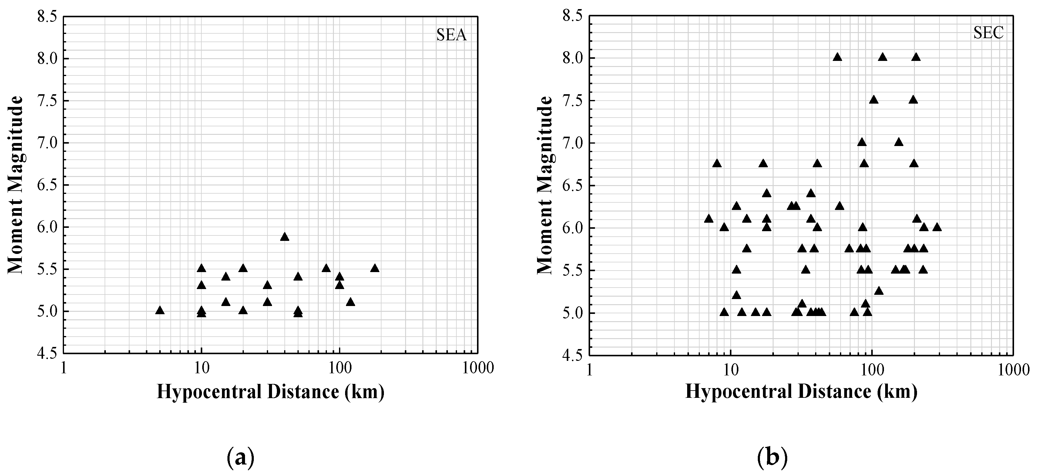
This paper is aimed at introducing a generic, regionally adjustable GMPE (known as the component attenuation model with acronym: CAM) for the prediction of PGV for given earthquake scenarios in low-to-moderate seismicity regions. The use of macroseismic historical MMI data collected from SEA and SEC regions (the distribution of magnitude and distance for collected data can be found in Figure 1) to demonstrate the accuracy of predictions by CAM is also presented.
2. The Component Attenuation Model (CAM) of PGV
The framework of CAM as a GMPE is defined in a generic functional form, which decouples the source and attenuation effects into different components, as shown by Equation (1).
Equation (1) can also be presented in the logarithmic (base 10) format as shown by Equation (2):
where is the referenced PGV measured on reference hard rock sites (typifying Eastern North America) for the reference scenario of M = 6 and R = 30; is the source factor, which is a function of the moment magnitude (M) and Brune stress drop (); is the regional anelastic attenuation factor, which is responsible for the attenuation effects, excluding geometric attenuation (G); G is the geometric attenuation factor; is the crustal modification factor, which accounts for the amplification and attenuation phenomena within the upper 4 km of the rock crust, as well as amplification at the “mid-crust”, which is in the surrounding of the location of the fault plane; and C is the calibration factor (which is used to minimise discrepancies between the model predictions and empirical recordings). The value of is set as unity (and value of and G close to unity) for a stress parameter value of 200 bars at M = 6 and R = 30 km. Seismological parameter values of stochastic simulations that CAM is based upon are summarised in Table 1. The listing of the values of model coefficients associated with each component factor in CAM are presented in the next section.
CAM, as introduced in the foregoing, is similar in methodology and philosophy to a generic ground motion prediction model (GMPE) introduced in reference [37]. A unique feature of CAM, which is not found in any GMPE, is the use of a geology-based crustal modelling approach, wherein crustal shear wave velocity profiles of bedrock to depths of tens of kilometres are used to derive modification factors of the upper crust (not to be confused with the site factor for modelling the effects of surficial sediments down to tens of metres only). Description of the crustal modelling methodology, complete with case studies, can be found throughout the rest of the article.
2.1. Generic Source Factor
The generic source factor is expressed in the form of Equation (3).
where – are model coefficients. Equation (3), which was derived from the simulated data, has been normalised at M = 6. The model covers the range of M4–M8 and = 30–300 bar.
2.2. Regional Whole Path Anelastic Attenuation Factor
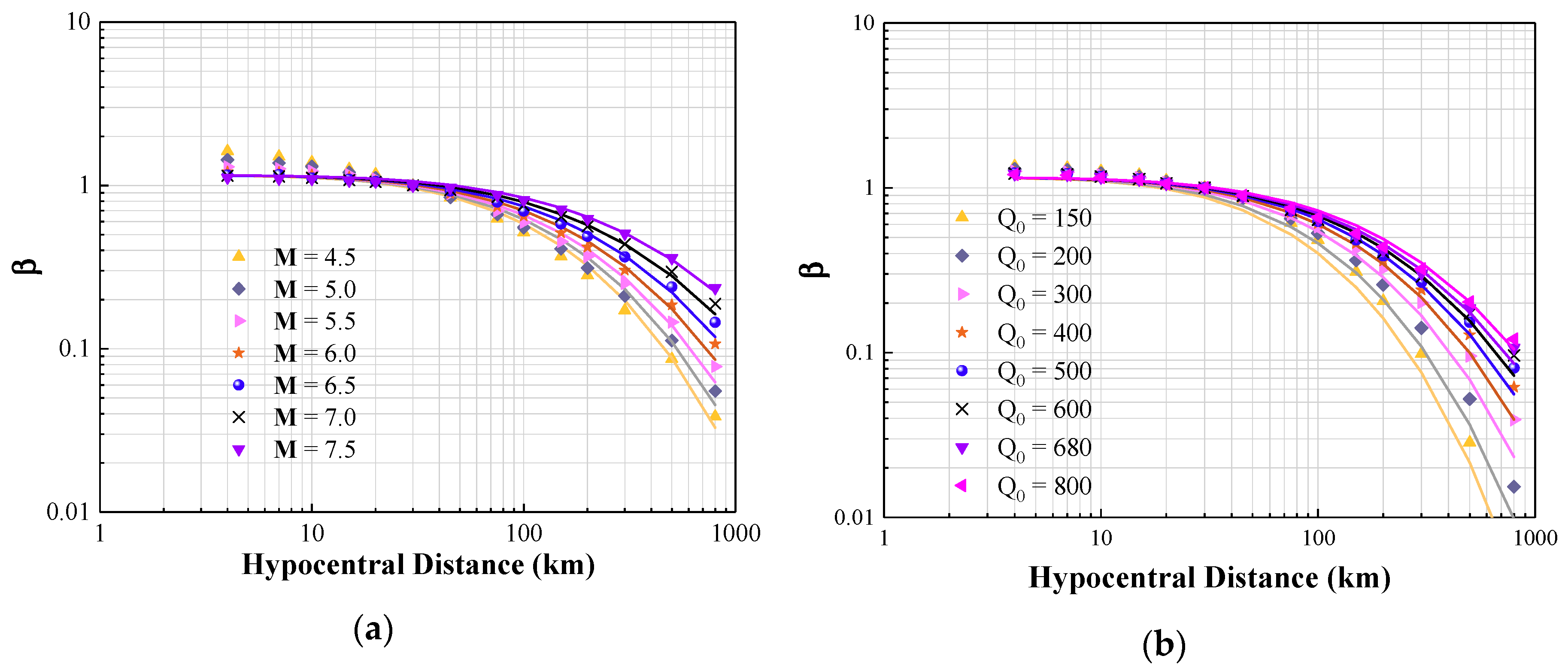
The regional anelastic attenuation factor () is used to account for the attenuation of ground motions along the entire transmission path of the seismic wave from source to site. Results derived from stochastic simulations of the seismological model with increasing distance have been normalised at R = 30 km and the effects of geometric attenuation effect (G) have been removed (and accounted for separately). The anelastic attenuation factor so derived is expressed in the form of Equation (4):
where – are model coefficients; M is moment magnitude, is the regional dependent quality factor for wave transmission, and R is the hypocentral distance.
Higher frequency waves (with a larger number of wave cycles for a given distance) are more susceptible to anelastic attenuation along the wave travel path than lower frequency waves. Given that the frequency characteristics of an earthquake are magnitude-dependent, the extent of anelastic attenuation is accordingly magnitude-dependent. Hence, earthquake magnitude is a parameter in the predictive expression of Equation (4). The reliability (ability) of this expression to reproduce results of stochastic simulations of the upper crustal amplification phenomenon reasonably accurately is demonstrated in Section 3.
Predictions derived from Equations (3) and (4) have been subject to residual analysis, wherein the residual value is defined as , where and are PGV measurements obtained from stochastic simulations and CAM predictions, respectively. > 0 refers to underestimation of CAM and < 0 refers to overestimation of CAM. A fourth order polynomial expression (Equation (5)) for defining the value of the adjustment factor is used to adjust, through multiplication, predicted values of β from Equation (4) to minimise the values of the residuals, along with any other systematic modelling errors.
where – are model coefficients.
2.3. Crustal Modification Factor
The crustal factor is to account for the combined effects of the amplification and attenuation of the upper earth crust, which is mainly dependent on the shear wave velocity profile in the upper 3–4 km of the earth crust. The literature refers to those phenomena as crustal modifications. The modification factor can be resolved into three components: (i) amplification of the upper crust; (ii) attenuation of the upper crust; and (iii) modification of the mid-crust. The respective factors representing each of these components are combined in a multiplicative manner, as represented by Equation (6).
where , , and are factors representing amplifications of the upper crust, attenuation of the upper crust, and modification of the mid-crust, respectively.
Details of the derivation of each of these component factors contributing to crustal modifications are described in the rest of this section under separate subheadings.
2.3.1. Upper-Crustal Amplification
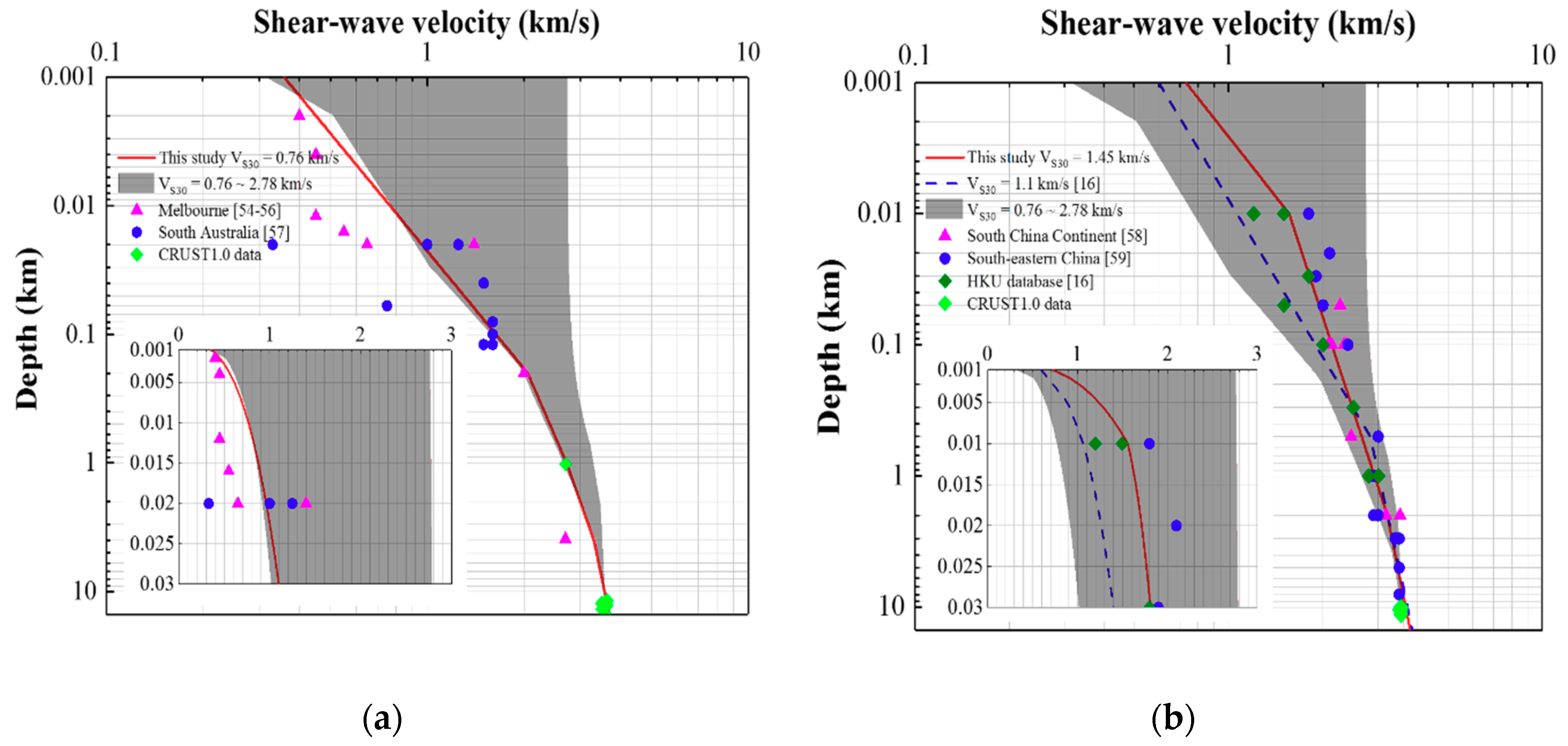
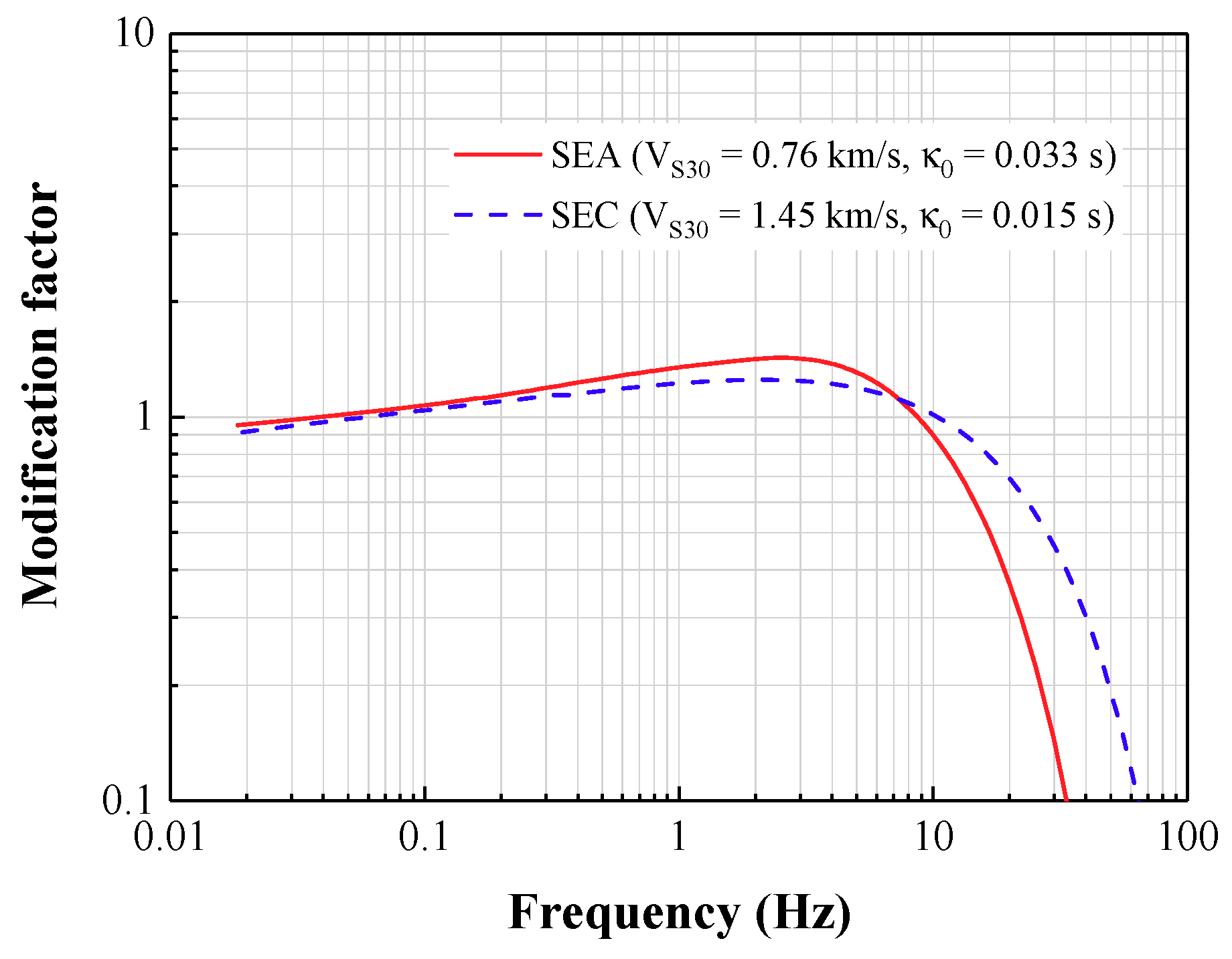
In modelling upper crustal amplification, information presented in reference [38], which is abbreviated herein as BJ97, and more recent updates of the model [39], have been incorporated for constructing the shear wave velocity profiles, which have also been used to infer the crustal density profiles [40]. The two profiles were then called up jointly to derive the upper crustal amplification factors by use of the square-root-impedance (SRI) method. The shear wave velocity profiles and the corresponding frequency-dependent amplification factors, so derived for the study regions, are presented in Figure 2 and Figure 3.
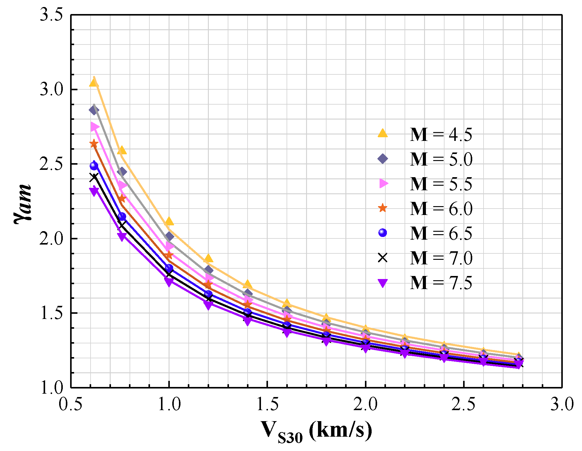
The upper-crustal amplification factor was derived accordingly as a function of (time-averaged shear wave velocity in the upper 30 m of the earth crusts [41]) by curve-fitting simulated data. The general form of the function is shown by Equation (7):
where – are the regression coefficients.
Upper crustal amplification of seismic waves is also frequency-dependent, given that the amplification of higher frequency waves (of shorter wave lengths) are more sensitive to the shear wave velocity gradient of the earth crust than lower frequency waves (of longer wave lengths). This phenomenon can be explained by reference to the quarter wavelength principles in the analysis for crustal amplification. Further explanations can be found in reference [38]. The extent of upper crustal amplification is accordingly dependent on the frequency characteristics of the upward propagating seismic waves. Given that the frequency characteristics of an earthquake are magnitude dependent, the extent of upper crustal amplification is, therefore, also magnitude dependent. Hence, earthquake magnitude is a parameter in the predictive expression of Equation (7). The validity of using VS30 to characterise upper crustal conditions has been demonstrated in reference [42]. The reliability (ability) of Equation (7) to reproduce results of stochastic simulations of the upper crustal amplification phenomenon reasonably accurately is demonstrated in Section 3.
2.3.2. Upper Crustal Attenuation
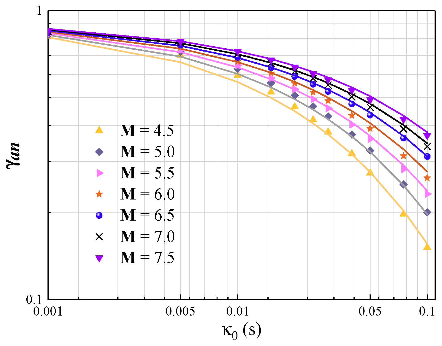
The Kappa factor ) is another key parameter to be considered in upper crustal modelling. The attenuation behaviour of the ground motion in the upper crust at high frequencies (in addition to the whole path anelastic attenuation covered in Section 2.2) is controlled by the value of . Numerous studies that were targeted at modelling the value of have been reported in the literature [41,42,43,44,45,46]. In simulations undertaken in this study, the value of accordingly ranges from 0.001 s to 0.1 s. The functional form for the expression for determining the values of to account for the effects of upper crustal attenuation is represented by Equation (8).
where – are regression coefficients.
As for whole path anelastic attenuation, upper crustal attenuation is also magnitude-dependent. Thus, earthquake magnitude is also a parameter in Equation (8) for predicting the extent of upper crustal attenuation. The significance of the magnitude term is well demonstrated in Section 3.
Residual analysis has been conducted for CAM in totality, incorporating the generic source, regional path (including anelastic and geometric attenuation factors), and crustal modification factor. An apparent trend with increasing distance R has been identified. A fourth order polynomial expression (Equation (9)) for defining the value of the adjustment factor is used to adjust, through multiplication, predicted values of PGV from Equation (3), (4), (5), (7), and (8) to minimise values of the residuals, along with other systematic modelling errors.
where – are regression coefficients.
2.3.3. Mid-Crustal Modification
Another crustal factor to consider is the mid-crustal modification factor , which is used to account for the effects of the density and shear wave velocity of the earth crust at the depth of the source of the earthquake. Mid-crustal amplification is purely a source phenomenon, as it represents the increase in the amplitude of shear waves (generated at the source of the earthquake) with decreasing shear wave velocity and density of the earth crust at the depth of the source from where seismic waves are emitted. In calculating the amplification factor a high shear wave velocity value of 3.8 km/s and a crustal density value of 2.8 g/cm3, both of which are characteristics of hard rock conditions in the shield regions of Eastern North America, are used as the “benchmark” conditions, for which the amplification factor is set as unity. These benchmark parameters for shear wave velocity and crustal density are denoted as and respectively.
The value of can be found using Equation (10), which has been derived by the authors based on the source model defined in reference [35].
where , = 2.8 g/cm3, = 3.8 km/s, and and are the density and shear wave velocity of the earth crust at the depth of the source (i.e., the mid-crust).
2.4. Verification of CAM Using Various Seismological Models
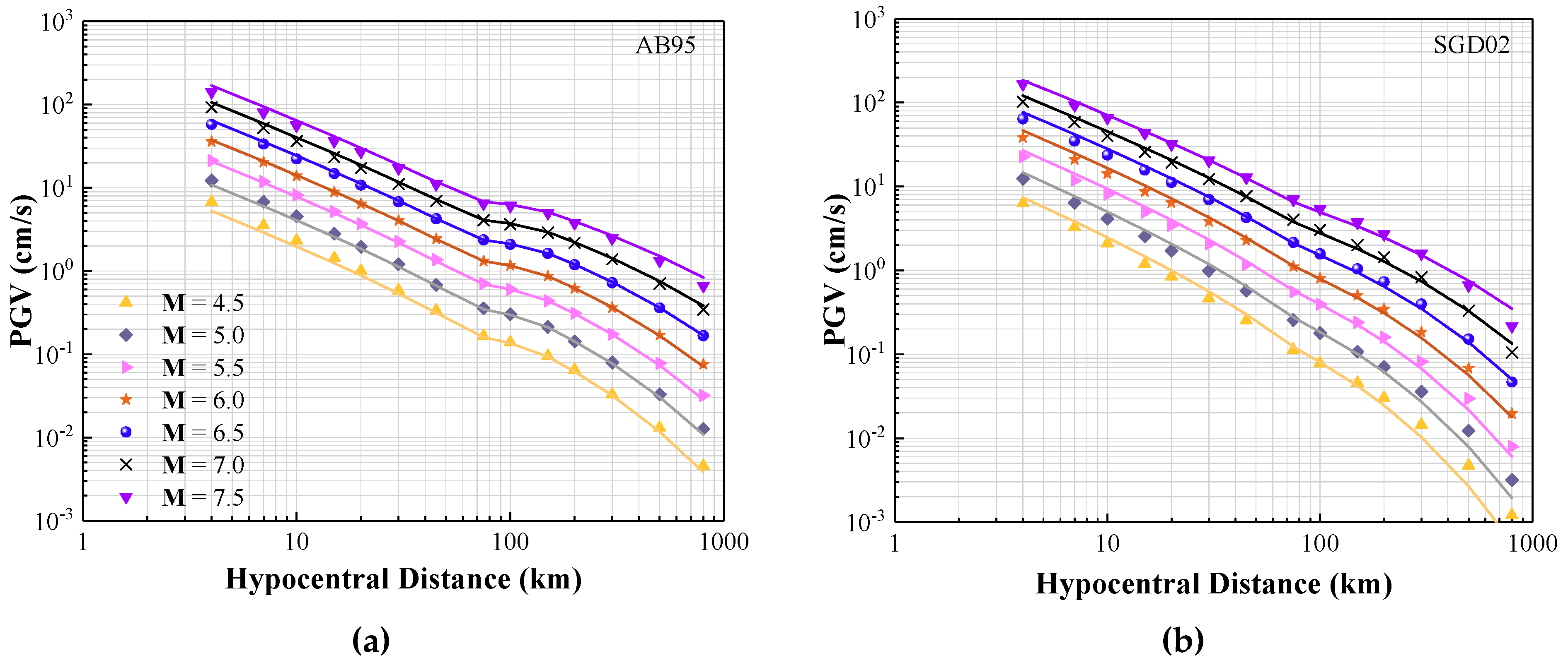
To verify CAM as a tool for translating seismological models into GMPEs for predictions of PGV, four NGA(Next Generation Attenuation)-East seismological models (as listed in Table 2), namely Atkinson and Boore (1995) [1], Silva, Gregor, and Darragh (2002) [47], Atkinson (2004) [48], and Boatwright and Seekins (2011) [49], have been used to verify CAM. The acronyms of these four models are AB95, SGD02, A04, and BS11. The PGV values, so derived from stochastic simulation of the (selected) seismological models, were compared with PGV values predicted by use of CAM for the respective model. Results of the verification analyses are presented in Section 3.2.
2.5. Validation of CAM Using MMI Data
Historical macroseismic MMI data collected from South-Eastern Australia (SEA) and South-Eastern China (SEC) has also been adopted to validate CAM as a regionally adjustable generic GMPE. The magnitude and distance distributions are shown in Figure 1 for the two selected study regions. The well-known MMI-PGV correlation proposed by Atkinson and Kaka [23] was adopted in this study (with residual corrections) to transfer the predicted PGV values (as derived from CAM) into MMI values for comparison purposes. The correlation relationship without residual corrections is expressed by Equation (11), and that with residual corrections is expressed by Equation (12). The historical MMI data can be found in this paper in the section presenting “Supplementary Materials”.
where M and R are the moment magnitude and hypocentral distance, respectively, and the unit of PGV is cm/s.
For recordings collected from SEA, some of the events were recorded in terms of local magnitude (ML). The conversion between M (moment magnitude, same as MW) and ML would need to be undertaken in the first place to obtain correct estimates of the event magnitude. In this study, the bilinear conversion relationship developed for Australian conditions [50] as defined by Equation (13) was adopted.
As the earthquake recordings for SEC were derived originally from the ancient yearbook, some records dated back to as early as the 15th century [51,52]. Thus, magnitude conversion is filled with uncertainties. The magnitude recordings compiled in this study (which can be found in the section titled “Supplementary Materials”) are expressed in terms of moment magnitude.
Another important component in CAM is the upper crustal modification factor. Regional shear wave velocity (SWV) profiles can be used for deriving the upper crustal amplification factor. The shear wave velocity profiles in this study were constructed based on the use of a geology-based modelling approach, as recommended in reference [53]. With this modelling approach, a compressional (P) wave velocity profile is converted into a shear (S) wave velocity profile using relationships that have been developed by regression analysis of recorded data collated from multiple sources. More details in relation to the process of modelling the shear wave velocity profile for the two study regions can be found in the “Supplementary Materials” section. The parameter values used for constructing SWV profiles are listed in Table 3. In Table 3, the values of ZS (depth of the upper sedimentary crustal layer) and ZC (combined thickness of the soft and hard sedimentary crustal rock layers) for each region were obtained from the average estimates of the thickness of soft sediment layer and total sediment layers, respectively, in CRUST1.0 database (https://igppweb.ucsd.edu/~gabi/crust1.html, last accessed in January 2019). VS0.03 (shear-wave velocity values at the depth of 0.03 km) values were identified by curve-fitting to minimise discrepancies (defined as sum of squares errors) between the modelled and recorded SWV values. The SWV value at 8 km depth (VS8), representing conditions at the source of the earthquake, has also been determined for the two study regions based on information of the regional crustal structure. The detailed information about the recorded SWV value can be found the references [54,55,56,57,58,59]. The velocity profile showing the upper bound of 2.78 km/s in Figure 2 is the shear wave velocity profile for generic hard rock conditions, as recommended in reference [38]. The velocity profile showing the lower bound of 0.76 km/s in Figure 2 was derived from interpolation between the shear wave velocity profiles for generic rock and generic hard rock conditions, as recommended in reference [38]. The modelling approach introduced in reference [39] has been adopted. The frequency-dependent modification factors for the study regions are shown in Figure 3.
The parameter values used in CAM and the selected GMPEs for comparison purposes for SEA and SEC regions are summarised in Table 4.
3. Results of Verification Analyses
3.1. PGV Modelling
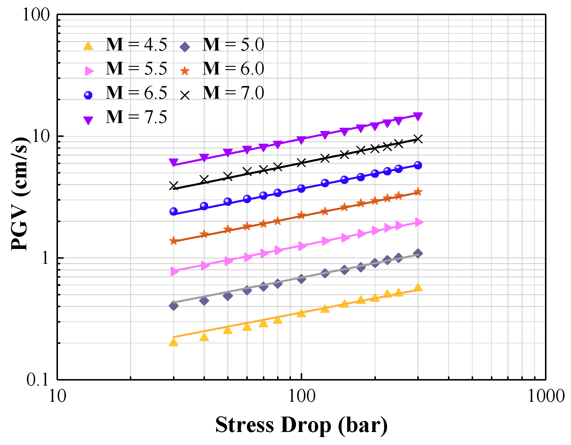
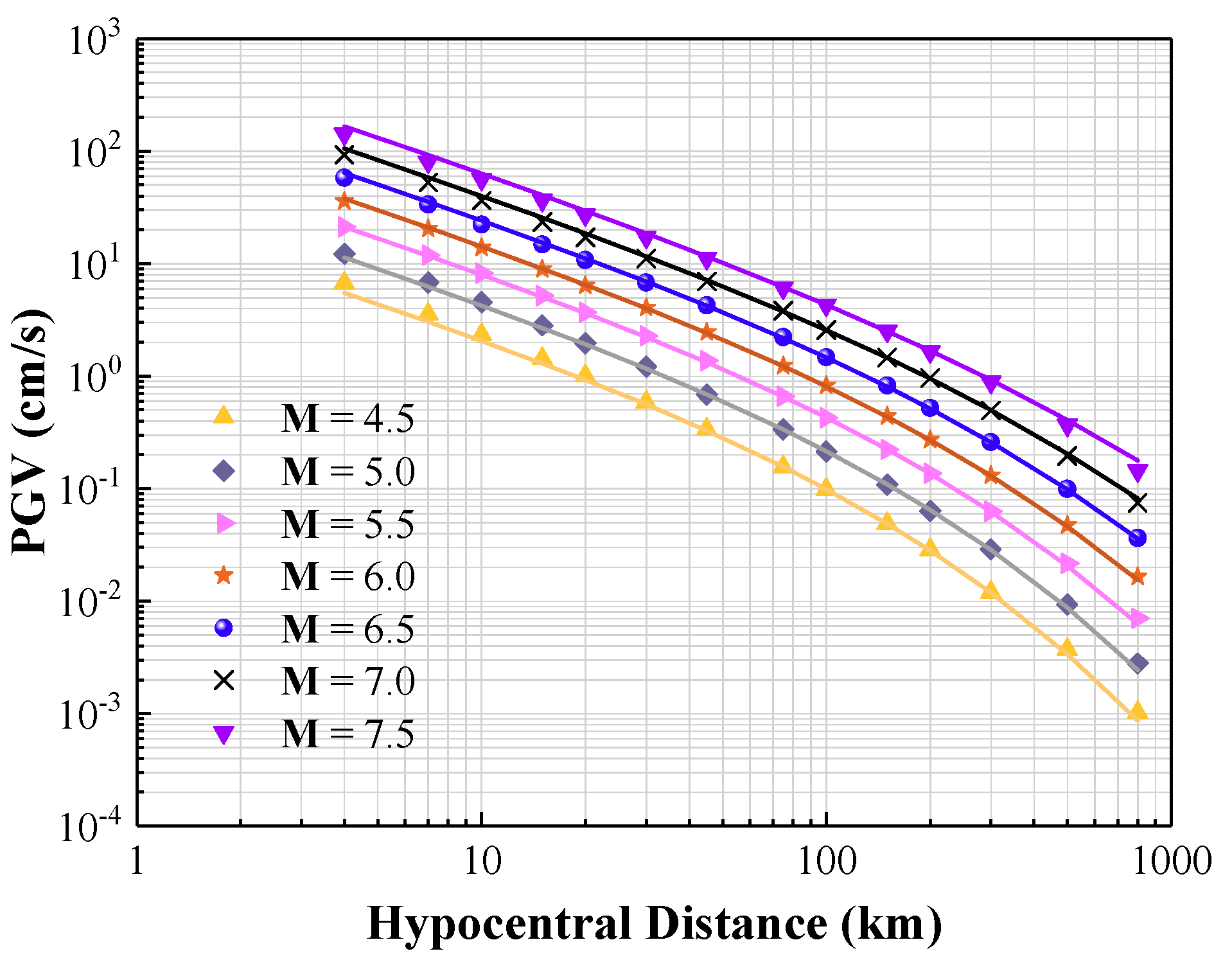
Values for each of the component factors in CAM are presented in, Figure 4, Figure 5, Figure 6, Figure 7 and Figure 8, alongside results generated from stochastic simulations of the respective seismological model. Figure 4 shows the source factor (α) as a function of M and ∆σ.
Figure 5 shows the path factor (β) as a function of moment magnitude M, R, and wave transmission quality factor (). Figure 6 shows the upper crustal amplification factor () as a function of M and VS30. Figure 7 shows the upper crustal attenuation factor () as a function of M and . Figure 8 shows the overall PGV obtained both from stochastic simulations and CAM predictions. The regression coefficients together with the regression goodness (R2) values for different component factors demonstrating excellent agreement between the two sets of results are summarised in Table 5.
This paper focuses on the use of CAM for predictions of PGV. CAM also provides predictions for response spectral accelerations. Refer to “Supplementary Materials”, which provides the link to access CAM for response spectrum modelling.
3.2. Translating Seismological Models into GMPEs in Terms of PGV
Four well-known NGA-East seismological models (as listed in Table 2) have been used as examples to verify the accuracy of CAM. The selected seismological models are namely Atkinson and Boore (1995) [1], Silva, Gregor, and Darragh (2002) [47], Atkinson (2004) [48], and Boatwright and Seekins (2011) [49], with acronyms: AB95, SGD02, A04, and BS11. Each of these models has its own attenuation properties (encompassing geometric attenuation and whole path anelastic attenuation). In this study, the same generic source factor (of the generalised additive double-corner frequency form with stress drop of 200 bar) and site conditions (VS30 = 0.76 km/s and = 0.025 s) have been input into the seismological models for defining the Fourier amplitude spectrum (FAS) and for making predictions of PGV through stochastic simulations. All the selected seismological models have been translated into PGV predictive models with a reasonable level of accuracy (as shown in Figure 9).
The process of transforming a seismological model into a ground motion prediction model is summarised as follows: (a) stochastic simulations of a seismological model based on a given set of seismological parameters for generating an ensemble of accelerograms, each of which has its own array of random phase angles; (b) calculation of the response spectrum for every accelerogram that has been generated; (c) statistical analysis of the calculated response spectral ordinates for determining their mean values; and (d) developing a GMPE for providing median ground motion predictions by collation of the mean response spectral values (across the natural period range of engineering interests) for different combinations of seismological parameters including M and R.
3.3. Comparing with Historical MMI Data and Existing GMPEs
In regions of low-to-moderate seismicity where instrumented strong motion data are lacking, ground motion models can be verified by use of macroseismic data. The most commonly used metrics of this type are modified Mercalli intensity (MMI) data. A more recently developed alternative to the MMI scale is the environmental seismic intensity (ESI) scale. Further descriptions of the ESI scale can be found in Section 4. At present, only data presented in the MMI scale are currently available in the two study regions for verifying CAM.
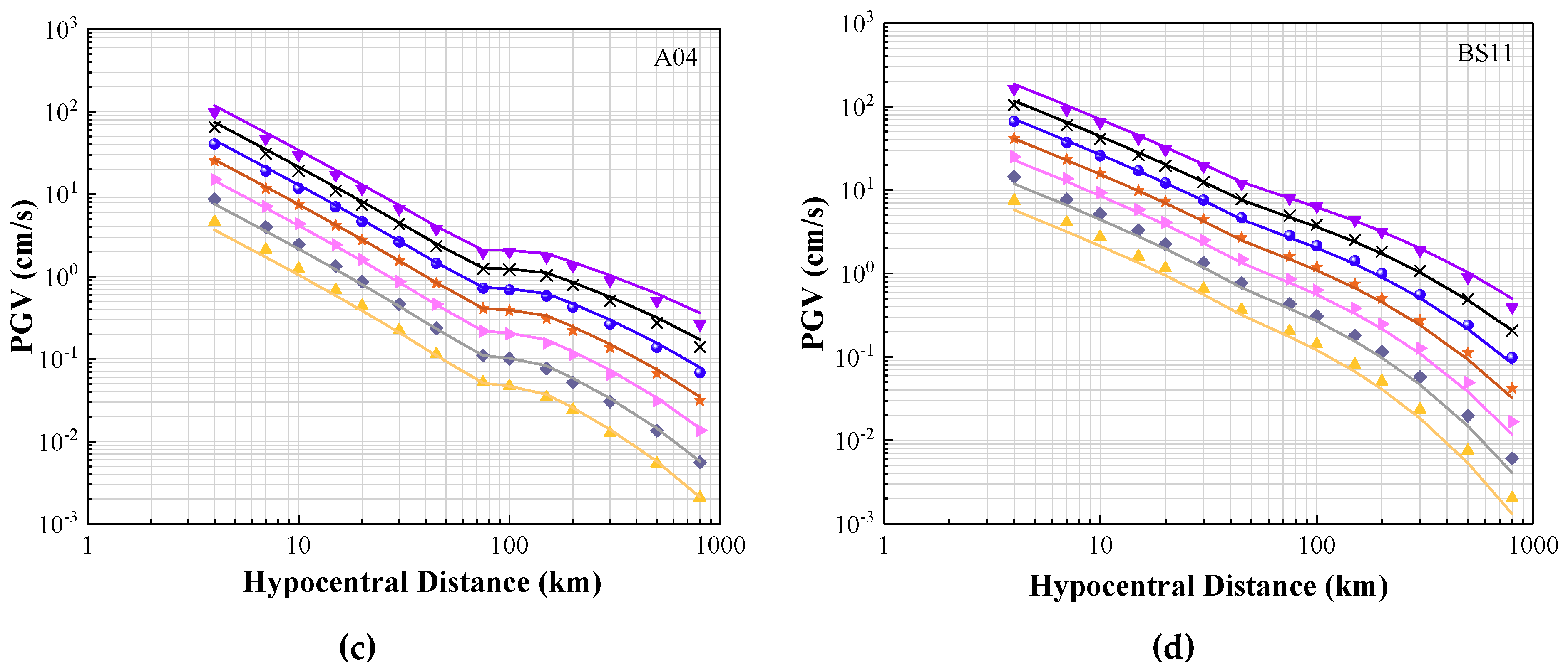
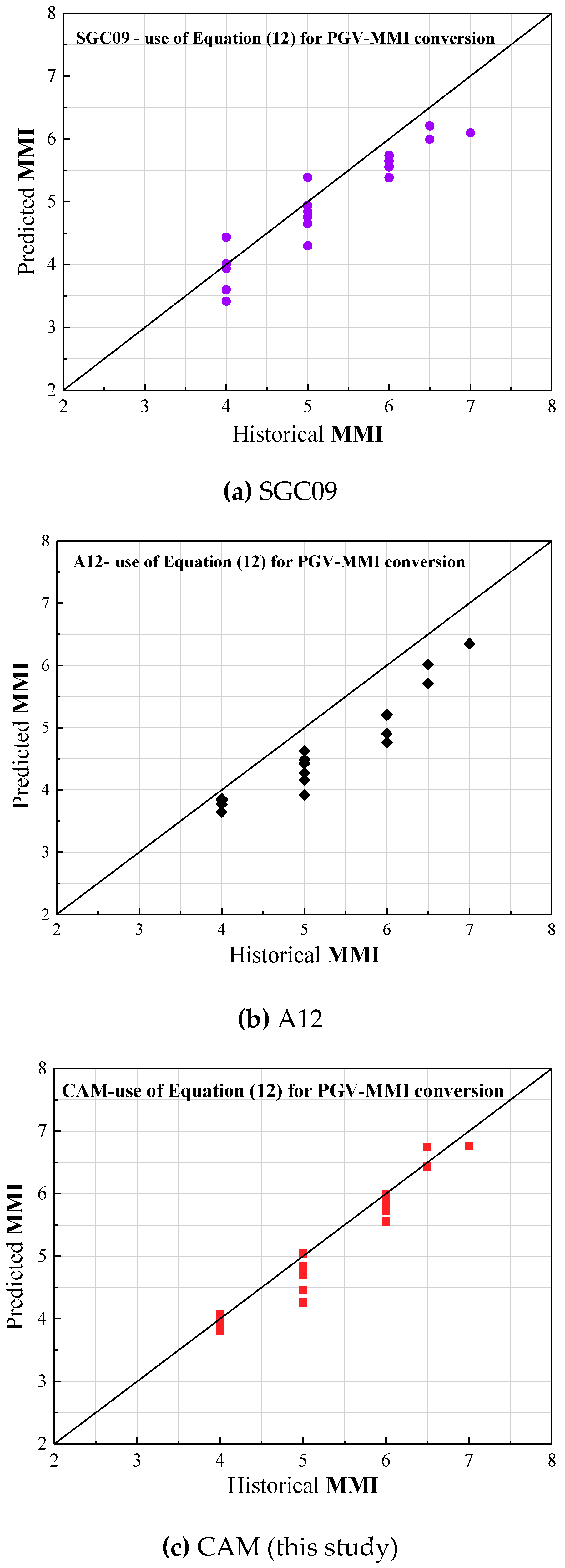
Four candidate GMPEs have been selected for use in the comparative study for evaluating the accuracies of GMPEs in terms of their level of agreement with MMI data. For modelling PGVs in SEA, GMPEs that have been compared are namely: (i) SGC09 (non-cratonic condition) [65], (ii) A12 (shallow earthquake) [18], and (iii) CAM-SEA (this study). For modelling PGVs in SEC, GMPEs that have been compared are namely: (i) CB08 [66], (ii) CY08 [2], and (iii) CAM-SEC (this study). CB08 model and CY08 model are selected because that PGV predictions by these two models have been suggested in the literature to be appropriate for use in South China [61,62]. Details of seismological parameters that have been identified for the two regions for input to CAM can be found in Table 4. Results of evaluations for the two regions are presented in Figure 10 and Figure 11, respectively. In both figures the x-axis is the historical recorded MMI values based on observations on average soil sites (as presented in “Supplementary Materials”). The y-axis shows the MMI values that are predicted from the four candidate GMPEs and have incorporated an average site factor of 1.5 for transforming predictions from rock sites to average soil sites. The key reference for sourcing intensity information from isoseismal maps was AGSO (1995) [67]. Information presented in website: https://earthquakes.ga.gov.au/ has also been used to identify locations of epicentres of the historical earthquake events.
4. Discussion
CAM essentially decouples the effect of earthquake source, path, and crust into separate components, thereby enabling it to be regionally adjustable in order that predictions for SEA and SEC can be covered in one model.
In Figure 9, all the simulated results (symbols) and predictions by CAM (lines) are shown to match well for the selected magnitude ranges, indicating that CAM can accurately represent the four selected seismological models: AB95, SGD02, A04, and BS11. The minor mismatch, as displayed in the figures, can be explained by the different relationships that have been used to determine the value of the exponent factor n in the function ( = ), as recommended in the literature; refer to reference [36]. A prominent feature of the A04 model is that the function for determining the factor is not of the typical form involving parameters and n, but is instead defined as: ). The strategy of setting = 893 for all Tn < 1.0 s, and = 1000 for all Tn ≥ 1.0 s has been adopted in predicting response spectral values. According to Bommer and Alarcon [25], the ratio between response spectral acceleration (RSA) and PGV (RSA/PGV) is nearly constant at Tn = 0.5 s, thus, = 893 was adopted in CAM for predicting the value of PGV in this study.
By a rough glance at Figure 10, predictions by CAM for SEA (Figure 10c) are shown to be in better agreement with the recorded values for MMI than the other two candidate GMPEs (Figure 10a,b). Adopting the geometric attenuation factor of R−1.33, as per recommendations by A12 [18], at short distance as opposed to the conventional factor of R−1 is controversial, whilst good match between the model predictions and field recorded data has been demonstrated in references [18,19]. It is noted that when calibrating seismological parameters (to achieve agreement between predictions from a seismological model and field recorded data) there are trade-offs of the assumed stress drop values with the assumed rate of geometrical attenuation. Stress drop behaviour of earthquakes, as assumed by different groups of investigators (based on calibration), can be very inconsistent. The geometrical factors adopted by the two study groups can accordingly be very inconsistent too (R−1.33 versus R−1), whilst achieving good agreement between predictions and recorded data in their respective studies.
Specific studies on ground motion characteristics of the SEC region have not been reported in the literature. In this study, the geometric attenuation form was adopted from AB95 model to represent the attenuation characteristics in the SEC region. CB08 [66] and CY08 [2] models were selected for comparison purpose, given that PGV predictions by these two models have been suggested in the literature to be appropriate for use in South China [61,62]. There appears to be under-predictions by CAM for SEC (Figure 11c), warranting further investigations whilst overpredictions by the other two models are also shown (Figure 11a,b).
Discrepancies of results presented in this study are considered to have been resulted from the following causes:
- Uncertainties with the relationship for conversion from MMI to PGV: Although the adopted MMI–PGV conversion function is recommended by many studies, there are still significant variances when applying the function to a diversity of regions, which is demonstrated by the discrepancies between not using residual corrections (Equation (11)) and using residual corrections (Equation (12)) in the relationship functions shown in Figure 10 and Figure 11.
- Uncertainties with the modification factor for conversion from MMI on a soil site to MMI on a rock site: a factor of 1.5 was adopted for both SEA (recommended by AS1170.4-2007 [64]) and SEC region (recommended by Tsang et al. [16]). CAM can only give predictions on rock sites and thus the conversion between soil sites and rock sites is essential.Uncertainties with magnitude conversion: in SEA, local magnitude (ML) has been converted into moment magnitude (M) based on studies conducted by Geoscience Australia [50]. However, the magnitude of ancient recordings in SEC has not been assured (the magnitude identified with individual recordings is assumed to be in moment magnitude).
- Uncertainties with shear wave velocity profiling: a geology-based approach for constructing SWV profile was adopted. This approach can make the best use of local recording data, thereby minimising inter-regional variability when calculating the upper crustal modification factor. For SEA region, the proposed SWV profile resulted in a VS30 value that is the same as previous study (0.76 km/s) [68]. However, for SEC region, the SWV profile obtained from this study (VS30 = 1.45 km/s) is different from that presented by Tsang et al. [16] (VS30 = 1.1 km/s, which is different from VS0.03). More local data for accurate SWV profile modelling is required in future studies.
- Uncertainties with the seismological parameters: no complete seismological model has been developed specifically for the SEC region. The parameter values (including stress drop value and geometric attenuation factor) used in CAM are mainly default values that are expected for a typical intraplate region.
- Another intrinsic limitation of CAM is that it has not taken earthquake duration effects into account in a comprehensive manner. Incorporating an adjustment factor for earthquake duration effects into CAM is recommended for its future development.
Another matter of consideration is the selection of the best metrics for quantifying the intensity of earthquake ground shaking (and ground deformation) in historical, and prehistorical, earthquake events. The most commonly used macroseismic intensity metrics is the MMI scale that has been used for verifying the accuracy of CAM, as described in the previous section of the article. A review of metrics presented in the MMI scale for quantifying historical earthquake hazards can be found in Ref. [24]. The alternative environmental seismic intensity scale (ESI) [69] is a new macroseismic metric that is based on traces left on the landscape that were caused by earthquake activities in the natural environment. ESI allows the intensity of ground shaking in an earthquake event to be post-dicted in situations where no information on damage to buildings is available or when diagnostic damage-based elements have saturated [70]. Thus, prehistorical events that are not within the scope of any historical archives can be covered. The basic idea of the ESI is to make use of traces of geological and/or geomorphological nature that have been left behind by primary and secondary surface ruptures and mass movements, so generated by large magnitude earthquakes to post-estimate the intensity of the hazard and the magnitude of the event [71]. Example applications of the ESI scale can be found in references [71,72,73,74,75]. Results reported in reference [73] indicate that incorporating ESI data into probabilistic/deterministic seismic hazard analysis can result in significant changes to the modelled PGA values. Another type of macroseismic information is paleo liquefaction data, which can also be employed to provide very valuable information in support of seismic hazard analyses [76].
5. Conclusions
CAM was introduced as an engineering tool for providing realistic ground motion predictions for intraplate regions. The modelling principle is based on utilising up-to-date (and generic) knowledge on the frequency behaviour of seismic waves that radiated from the source of a local (small and medium magnitude) earthquake in combination with knowledge on local geophysical and crustal conditions, which control frequency modifications along the wave travel path. The seismological model provides the framework for integrating both knowledge bases into the predictions. This decoupling approach to modelling is more scientific, and rational, than simply applying the logic tree procedure to assign weighing factors on existing ground motion models (that are typically biased to conditions and areas where instrumented data are abundant).
This article focused on PGV as a ground motion intensity metric that can be translated into MMI data (which can be compared with data extracted from isoseismal maps of historical earthquake events). The use of algebraic expressions to make predictions of the PGV is an important feature in CAM. Essentially, an adaptable seismological model is presented as a GMPE, thereby waiving away the need for undertaking stochastic simulations along with response spectral computations. An important, and significant, achievement of this article was to have the algebraic expressions in CAM verified. The outcome from the MMI comparative study undertaken for SEA also shows a great deal of promise for CAM, but there are also scopes of improving the match with SEC data in a future study.
The user-friendly setting of CAM (featuring the use of algebraic expressions) serves to facilitate engineering professionals to become more involved with ground motion modelling, thereby gaining a good perspective of the modelling rationale and the underlying assumptions. In summary, this article represents a contribution towards improving transparencies in seismic hazard modelling and in the selection, and scaling of, accelerograms for engineering applications.
The success of CAM in the future relies on the investment of resources into studying crustal and geophysical conditions in intraplate regions for the users of CAM become better informed. This is important given that the quality of the output from any predictive model can only be as good as the quality of input into the model. Further investigations on the MMI-PGV conversion relationship are also warranted for comparison across GMPE models involving the use of MMI data to become more robust.
Supplementary Materials
Supplementary materials can be found at https://www.mdpi.com/2076-3263/9/10/422/s1. The detailed information about the proposed geology-based shear wave modelling approach is available online at: https://www.dropbox.com/s/jp4o7j08fe3gqxn/Geology-based-SWV-modelling.pdf?dl=0. The MMI recordings for the SEA region can be found online at: https://www.dropbox.com/s/v3eqh3w686ho97j/MMI%20events%20SEA.xlsx?dl=0. The MMI recordings for the SEC region can be found online at: https://www.dropbox.com/s/8vr4wq9mbsee5c0/MMI%20Events%20SEC.xlsx?dl=0. The vs. data can be found online at: https://www.dropbox.com/s/u3v127wjt10cwwk/Shear%20wave%20velocity%20data.xlsx?dl=0. The link to access CAM for response spectrum modelling: https://www.dropbox.com/s/jjfbfc8cm2srub3/CAM-Response-spectral-acceleration.pdf?dl=0.
Author Contributions
Conceptualization, N.L., H.-H.T., and Y.T.; methodology, Y.T., H.-H.T.; software, Y.T.; validation, Y.T. and N.L.; formal analysis, N.L., Y.T.; investigation, Y.T., N.L.; resources, Y.T.; data curation, N.L., H.-H.T., and Y.T.; writing—original draft preparation, Y.T.; writing—review and editing, N.L., H.-H.T., and E.L.; visualization, Y.T.; supervision, N.L., H.-H.T., and E.L.; project administration, N.L.; funding acquisition, N.L.
Funding
The first author was funded by China Scholarship Council, CSC grant number 201506030102. The project was funded by Commonwealth of Australia through the Cooperative Research Centre program.
Acknowledgments
The extensive technical support given by Yiwei Hu at the University of Melbourne is gratefully acknowledged.
Conflicts of Interest
The authors declare no conflict of interest.
References
- Atkinson, G.M.; Boore, D.M. Ground-motion relations for Eastern North America. Bull. Seism. Soc. Am. 1995, 85, 17–30. [Google Scholar]
- Chiou, B.J.; Youngs, R.R. An NGA model for the average horizontal component of peak ground motion and response spectra. Earthq. Spectra 2008, 24, 173–215. [Google Scholar] [CrossRef]
- Brune, J.N. Tectonic stress and the spectra of seismic shear waves from earthquakes. J. Geophys. Res. 1970, 75, 4997–5009. [Google Scholar] [CrossRef] [Green Version]
- Atkinson, G.M.; Boore, D.M. Earthquake ground-motion prediction equations for Eastern North America. Bull. Seism. Soc. Am. 2006, 96, 2181–2205. [Google Scholar] [CrossRef]
- Hassani, B.; Atkinson, G.M. Adjustable generic ground-motion prediction equation based on equivalent point-source simulations: Accounting for kappa effects. Bull. Seism. Soc. Am. 2018, 108, 913–928. [Google Scholar] [CrossRef]
- Boore, D.M.; Stewart, J.P.; Seyhan, E.; Atkinson, G.M. NGA-West2 equations for predicting PGA, PGV, and 5% damped PSA for shallow crustal earthquakes. Earthq. Spectra 2014, 30, 1057–1085. [Google Scholar] [CrossRef]
- Campbell, K.W.; Bozorgnia, Y. NGA-West2 ground motion model for the average horizontal components of PGA, PGV, and 5% damped linear acceleration response spectra. Earthq. Spectra 2014, 30, 1087–1115. [Google Scholar] [CrossRef]
- Zafarani, H.; Mousavi, M.; Noozad, A.; Ansari, A. Calibration of the specific barrier model to Iranian plateau earthquakes and development of physically based attenuation relationships for Iran. Soil Dyn. Earthq. Eng. 2008, 28, 550–576. [Google Scholar] [CrossRef]
- Lam, N.T.K.; Wilson, J.L.; Hutchinson, G.L. Generation of synthetic earthquake accelerograms using seismological modelling: A review. J. Earthq. Eng. 2000, 4, 321–354. [Google Scholar] [CrossRef]
- Boore, D.M. Simulation of ground motion using the stochastic method. Pure Appl. Geophys. 2003, 160, 635–676. [Google Scholar] [CrossRef]
- Campbell, K.W. Prediction of strong ground motion using the hybrid empirical method and its use in the development of ground-motion (attenuation) relations in Eastern North America. Bull. Seism. Soc. Am. 2003, 93, 1012–1033. [Google Scholar] [CrossRef]
- Pezeshk, S.; Zandieh, A.; Campbell, K.W.; Tavakoli, B. Ground Motion Prediction Equations for CENA Using the Hybrid Empirical Method in Conjunction with NGA-West2 Empirical Ground Motion Models, in NGA-East: Median Ground Motion Models for the Central and Eastern North America Region; PEER Rept. No. 2015/04, Chapter 5; Pacific Earthquake Engineering Research Center: Berkeley, CA, USA, 2015; pp. 119–147. [Google Scholar]
- Atkinson, G.M. Ground-motion prediction equations for Eastern North America from a referenced empirical approach: Implications for epistemic uncertainty. Bull. Seismol. Soc. Am. 2008, 98, 1304–1318. [Google Scholar] [CrossRef]
- Hassani, B.; Atkinson, G.M. Referenced empirical ground-motion model for Eastern North America. Seism. Res. Lett. 2015, 86, 477–491. [Google Scholar] [CrossRef]
- Lam, N.T.K.; Sinadinovski, C.; Koo, R.; Wilson, J.L. Peak ground velocity modelling for Australian intraplate Earthquakes. J. Seismol. Earthq. Eng. 2003, 5, 11–21. [Google Scholar]
- Tsang, H.H.; Sheikh, M.N.; Lam, N.T.K.; Chandler, A.M.; Lo, S.H. Regional differences in attenuation modelling for Eastern China. J. Asian Earth Sci. 2010, 39, 441–459. [Google Scholar] [CrossRef] [Green Version]
- Noman, M.N.A.; Cramer, C.H. Empirical Ground-Motion Prediction Equations for Eastern North America; PEER Rept. No. 2015/04; Chapter 8; Pacific Earthquake Engineering Research Center, University of California: Berkeley, CA, USA, 2015; pp. 193–212. [Google Scholar]
- Allen, T.I. Stochastic Ground-Motion Prediction Equations for Southeastern Australian Earthquakes Using Updated Source and Attenuation Parameters; Geoscience Australia: Canberra, ACT, Australia, 2012. [Google Scholar]
- Allen, T.I.; Dhu, T.I.; Cummins, P.R.; Schneider, J.F. Empirical attenuation of ground-motion spectral amplitudes in Southwestern Western Australia. Bull. Seismol. Soc. Am. 2006, 96, 572–585. [Google Scholar] [CrossRef]
- Newmark, N.M.; Rosenblueth, E. Fundamentals of Earthquake Engineering; Prentice Hall Inc.: New Jersey, NJ, USA, 1971. [Google Scholar]
- Gaull, B.A.; Michael-Leiba, M.O.; Rynn, J.M.W. Probabilistic earthquake risk maps of Australia. Aust. J. Earth Sci. 1990, 37, 169–187. [Google Scholar] [CrossRef]
- Kaka, S.I.; Atkinson, G.M. Relationships between instrumental ground-motion parameters and Modified Mercalli Intensity in eastern North America. Bull. Seism. Soc. Am. 2004, 94, 1728–1736. [Google Scholar] [CrossRef]
- Atkinson, G.M.; Kaka, S.I. Relationship between felt intensity and instrumental ground motion in the Central United States and California. Bull. Seism. Soc. Am. 2007, 97, 497–510. [Google Scholar] [CrossRef]
- Yaghmaei-Sabegh, S.; Tsang, H.H.; Lam, N.T.K. Conversion between Peak Ground Motion Parameters and Modified Mercalli Intensity Values. J. Earthq. Eng. 2011, 15, 1138–1155. [Google Scholar] [CrossRef]
- Bommer, J.J.; Alarcon, J.E. The prediction and use of peak ground velocity. J. Earthq. Eng. 2006, 10, 1–31. [Google Scholar] [CrossRef]
- Akkar, S.; Ozen, O. Effect of peak ground velocity on deformation demands for SDOF systems. Earthq. Eng. Struct. Dyn. 2005, 34, 1551–1571. [Google Scholar] [CrossRef]
- Todorovska, M.I.; Trifunac, M.D. Hazard mapping of normalized peak strain in soils during earthquakes: Mircozonation of a metropolitan area. Soil Dyn. Earthq. Eng. 1996, 15, 321–329. [Google Scholar] [CrossRef]
- FEMA. FEMA’s Software Program for Estimating Potential Losses from Disasters; FEMA: Washington, DC, USA, 2003. [Google Scholar]
- Trifunac, M.D. Empirical criteria for liquefaction in sands via standard penetration tests and sesimic wave energy. Soil Dyn. Earthq. Eng. 1995, 14, 419–426. [Google Scholar] [CrossRef]
- Kostadinov, M.V.; Towhata, I. Assessment of liquefaction-inducing peak ground velocity and frequency of horizontal ground shaking at onset of phenomenon. Soil Dyn. Earthq. Eng. 2002, 22, 309–322. [Google Scholar] [CrossRef]
- Orense, R.P. Assessment of liquefaction potential based on peak ground motion parameters. Soil Dyn. Earthq. Eng. 2005, 25, 225–240. [Google Scholar] [CrossRef]
- Newmark, N.M.; Blume, J.A.; Kapur, K.K. Seismic design spectra for nuclear power plants. J. Power Div. ASCE 1973, 99, 287–303. [Google Scholar]
- Newmark, N.M.; Hall, W.J. Earthquake Spectra and Design; Earthquake Engineering Research Institute: El Cerrito, CA, USA, 1982. [Google Scholar]
- Wilson, J.L.; Lam, N.T.K.; Australian Earthquake Engineering Society. AS 1170.4-2007 Commentary: Structural Design Actions; Part 4, Earthquake Actions in Australia; Australian Earthquake Engineering Society: McKinnon, VIC, Australia, 2007. [Google Scholar]
- Boore, D.M.; Alessandro, C.D.; Abrahamson, N.A. A generalization of the double-corner-frequency source spectral model and its use in the SCEC BBP validation exercise. Bull. Seismol. Soc. Am. 2014, 104, 2387–2398. [Google Scholar] [CrossRef]
- Mak, S.; Chan, L.S.; Chandler, A.M.; Koo, R. Coda Q estimates in the Hong Kong Region. J. Asian Earth Sci. 2004, 24, 127–136. [Google Scholar] [CrossRef]
- Yenier, E.; Atkinson, G.M. Regional adjustable generic ground-motion prediction equation based on equivalent point-source simulations: Application to Central and Eastern North America. Bull. Seismol. Soc. Am. 2015, 105, 1989–2009. [Google Scholar] [CrossRef]
- Boore, D.M.; Joyner, W.B. Site amplification for generic rock sites. Bull. Seismol. Soc. Am. 1997, 87, 327–341. [Google Scholar]
- Boore, D.M. Short Note: Determining generic velocity and density models for crustal amplification calculations, with an update of the Boore and Joyner (1997) generic amplification for VS(Z) = 760 m/s. Bull. Seism. Soc. Am. 2016, 106, 316–320. [Google Scholar] [CrossRef]
- Brocher, T.M. Empirical relations between elastic wavespeeds and density in the earth’s crust. Bull. Seismol. Soc. Am. 2005, 95, 2081–2092. [Google Scholar] [CrossRef]
- Silva, W.J.; Darragh, R.B.; Gregor, N.N.; Martin, G.; Abragamson, N.A.; Kircher, C. Reassessment of Site Coefficients and Near-Fault Factors for Building Code Provisions; Final Technical Report; N.E.R. Program: El Cerrito, CA, USA, 1999. [Google Scholar]
- Chandler, A.M.; Lam, N.T.K.; Tsang, H.H. Near-surface attenuation modelling based on rock shear-wave velocity profile. Soil Dyn. Earthq. Eng. 2006, 26, 1004–1014. [Google Scholar] [CrossRef] [Green Version]
- Chandler, A.M.; Lam, N.T.K.; Tsang, H.H. Regional and Local Factors in Attenuation Modelling: Hong Kong Case Study. J. Asian Earth Sci. 2006, 27, 892–906. [Google Scholar] [CrossRef]
- Drouet, S.; Cotton, F.; Guéguen, P. VS30, κ, regional attenuation and MW from accelerograms: Application to magnitude 3–5 French earthquakes. Geophys. J. Inter. 2010, 182, 880–898. [Google Scholar] [CrossRef]
- Edwards, B.; Fäh, D.; Giardini, D. Attenuation of seismic shear wave energy in Switzerland. Geophys. J.Inter 2011, 185, 967–984. [Google Scholar] [CrossRef] [Green Version]
- Van Houtte, C.; Drouet, S.; Cotton, F. Analysis of the origins of κ (kappa) to compute hard rock to rock adjustment factors for GMPEs. Bull. Seismol. Soc. Am. 2011, 101, 2926–2941. [Google Scholar] [CrossRef]
- Silva, W.J.; Gregor, N.N.; Darragh, R.B. Development of Regional Hard Rock Attenuation Relations for Central and Eastern North America; Pacific Engineering and Analysis: El Cerrito, CA, USA, 2002. [Google Scholar]
- Atkinson, G.M. Empirical attenuation of ground motion spectral amplitudes in Southeastern Canada and the Northeastern United States. Bull. Seismol. Soc. Am. 2004, 94, 1079–1095. [Google Scholar] [CrossRef]
- Boatwright, J.; Seekins, L. Regional spectral analysis of three moderate earthquakes in Northeastern North America. Bull. Seismol. Soc. Am. 2011, 101, 1769–1782. [Google Scholar] [CrossRef]
- Ghasemi, H.; Allen, T.I. Testing the sensitivity of seismic hazard in Australia to new empirical magnitude conversion equations. In Proceedings of the AEES, Canberra, ACT, Australia, 24–26 November 2017. [Google Scholar]
- Gao, W.X. China Earthquake Yearbook; Seismological Press: Beijing, China, 1990. [Google Scholar]
- Gu, G.X. Catalogue of Chinese Earthquake (1831 B.C.–1969 A.D.); Science Press: Beijing, China, 1989. [Google Scholar]
- Chandler, A.M.; Lam, N.T.K.; Tsang, H.H. Shear wave velocity modelling in crustal rock for seismic hazard analysis. Soil Dyn. Earthq. Eng. 2006, 25, 167–185. [Google Scholar] [CrossRef]
- Lam, N.T.K.; Asten, M.W.; Chandler, A.M.; Tsang, H.H.; Venkatesan, S.; Wilson, J.L. Seismic attenuation modelling for Melbourne based on the SPAC-CAM Procedure. In Proceedings of the AEES, Mount Gambier, SA, Australia, 5–7 November 2004. [Google Scholar]
- Roberts, J.; Asten, M.; Tsang, H.H.; Venkatesan, S.; Lam, N.T.K. Shear Wave Velocity Profiling in Melbourne Silurian Mudestone Using the SPAC Method. In Proceedings of the AEES, Mount Grambier, SA, Australia, 5–7 November 2004. [Google Scholar]
- Lam, N.T.K.; Venkatesan, S.; Wilson, J.; Asten, M.; Roberts, J.; Chandler, A.; Tsang, H.H. Generic Approach for Modelling Earthquake Hazard. Adv. Struct. Eng. 2006, 9, 67–82. [Google Scholar] [CrossRef]
- Collins, C.; Kayen, R.; Carkin, B.; Allen, T.I.; Cummins, P.R.; McPherson, A. Shear Wave Velocity Measurement at Australian Ground Motion Seismometer Sites by the Spectral Analysis of Surface Waves (SASW) Method; Earthquake Engineering in Australia: Canberra, ACT, Australia, 2006. [Google Scholar]
- Zhao, B.; Zhang, Z.; Bai, Z.; Badal, J.; Zhang, Z. Shear Velocity and Vp/Vs Ratio Structure of the Crust beneath the Southern Margin of South China Continent. J. Asian Earth Sci. 2013, 62, 167–179. [Google Scholar] [CrossRef]
- Zhao, M.; Qiu, X.; Xia, S.; Xu, H.; Wang, P.; Tan, K.; Lee, C.; Xia, K. Seismic Structure in the Northeastern South China Sea: S-wave Velocity and Vp/Vs Ratios Derived from Three-component OBS Data. Tectonophysics 2010, 480, 183–197. [Google Scholar] [CrossRef]
- Zhang, Z.; Yang, L.; Teng, J.; Badal, J. An Overview of the Earth Crust Under China. Earth Sci. Rev. 2011, 104, 143–166. [Google Scholar] [CrossRef]
- Xie, J.; Li, X.; Wen, Z.; Wu, C. Near-Source Vertical and Horizontal Strong Ground Motion from the 20 April 2013 Mw 6.8 Lushan Earthquake in China. Seism. Res. Lett. 2014, 85, 23–33. [Google Scholar] [CrossRef]
- Megawati, K. Hybrid Simulations of Ground Motions from Local Earthquakes Affecting Hong Kong. Bull. Seismol. Soc. Am. 2007, 97, 1293–1307. [Google Scholar] [CrossRef]
- Standards Australia. Earthquake actions in Australia. In AS 1170.4-2007: Structural Design Actions; Standards Australia: Sidney, NSW, Australia, 2007. [Google Scholar]
- Lam, N.T.K.; Wilson, J.L. The new response spectrum model for Australia. Electron. J. Struct. Eng. 2008, 8, 6–24. [Google Scholar]
- Somerville, P.; Graves, R.; Collins, N.; Song, S.G.; Ni, S.; Cummins, P. Source and Ground Motion Models for Australian Earthquakes. In Proceedings of the AEES, Newcastle, NSW, Australia, 11–13 December 2009. [Google Scholar]
- Campbell, K.W.; Bozorgnia, Y. NGA ground motion model for the geometric mean horizontal component of PGA, PGV, PGD and 5% damped linear elastic response spectra for periods ranging from 0.01 s to 10 s. Earthq. Spectra 2008, 24, 139–171. [Google Scholar] [CrossRef]
- AGSO (Australian Geological Survey Organisation). Atlas of Iso-Seismal Maps of Australian Earthquakes; McCue, K., Ed.; Australian Geological Survey Organisation: Canberra, ACT, Australia, 1995. [Google Scholar]
- Allen, T.I.; Leonard, M.; Clark, D.; Ghasemi, H. The 2018 National Seismic Hazard Assessment for Australia-Model Overview; Clark, D., Ed.; Geoscience Australia: Canberra, ACT, Australia, 2018. [Google Scholar]
- Michetti, A.M.; Esposito, E.; Guerrieri, L.; Porfido, S.; Serva, L.; Tatevossian, R.; Vittori, E.; Audemard, F.; Azuma, T.; Clague, J.; et al. Intensity Scale ESI 2007. Mem. Descr. Carta Geol. 2007, 74, 11–20. [Google Scholar]
- Serva, L. History of the Environmental Seismic Intensity Scale ESI-07. Geoscience 2019, 9, 210. [Google Scholar] [CrossRef]
- Grützner, C.; Walker, R.; Ainscoe, E.; Elliott, A.; Abdrakhmatov, K. Earthquake Environmental Effects of the 1992 Ms7.3 Suusamyr Earthquake, Kyrgyzstan, and Their Implications for Paleo-Earthquake Studies. Geoscience 2019, 9, 271. [Google Scholar] [CrossRef]
- Chunga, K.; Livio, F.A.; Martillo, C.; Lara-Saavedra, H.; Ferrario, M.F.; Zevallos, I.; Michetti, A.M. Landslides Triggered by the 2016 Mw 7.8 Pedernales, Ecuador Earthquake: Correlations with ESI-07 Intensity, Lithology, Slope and PGA-h. Geoscience 2019, 9, 371. [Google Scholar] [CrossRef]
- Caccavale, M.; Sacchi, M.; Spiga, E.; Porfido, S. The 1976 Guatemala Earthquake: ESI Scale and Probabilistic/Deterministic Seismic Hazard Analysis Approaches. Geoscience 2019, 9, 403. [Google Scholar] [CrossRef]
- King, T.R.; Quigley, M.; Clark, D. Surface-Rupturing Historical Earthquakes in Australia and Their Environmental Effects: New Insights from Re-Analyses of Observational Data. Geoscience 2019, 9, 408. [Google Scholar] [CrossRef]
- Silva, P.G.; Rodríguez-Pascua, M.A.; Robles, J.L.G.; Élez, J.; Pérez-López, R.; Davila, M.B.B. Catalogue of the Geological Effects of Earthquakes in Spain Based on the ESI-07 Macroseismic Scale: A New Database for Seismic Hazard Analysis. Geoscience 2019, 9, 334. [Google Scholar] [CrossRef]
- Tuttle, M.P.; Hartleb, R.; Wolf, L.; Mayne, P.W. Paleo liquefaction Studies and the Evaluation of Seismic Hazard. Geoscience 2019, 311, 1–61. [Google Scholar]
Figure 1.
M-R combinations for selected regions. (a) South-Eastern Australia (SEA); (b) South-Eastern China (SEC).
Figure 1.
M-R combinations for selected regions. (a) South-Eastern Australia (SEA); (b) South-Eastern China (SEC).

Figure 2.
Shear-wave velocity profile: (a) SEA; (b) SEC, in which CRUST1.0 is a global crustal database (https://igppweb.ucsd.edu/~gabi/crust1.html, last accessed in January 2019), the shear wave velocity data can be found in the “Supplementary Materials”.
Figure 2.
Shear-wave velocity profile: (a) SEA; (b) SEC, in which CRUST1.0 is a global crustal database (https://igppweb.ucsd.edu/~gabi/crust1.html, last accessed in January 2019), the shear wave velocity data can be found in the “Supplementary Materials”.

Figure 3.
Frequency-dependent crustal modification factor. For both conditions, κ0 = 0.057/− 0.02 [42,43].

Figure 4.
Simulated values of peak ground velocity (PGV) (symbols) alongside predictions by CAM (lines) for varying moment magnitudes (M4.5–M7.5) and stress drops (30–300 bar), at R = 30 km.
Figure 4.
Simulated values of peak ground velocity (PGV) (symbols) alongside predictions by CAM (lines) for varying moment magnitudes (M4.5–M7.5) and stress drops (30–300 bar), at R = 30 km.

Figure 5.
Anelastic attenuation factor (β). (a) Simulated PGV values normalised at = 680 for varying M values (M4.5–M7.5) and distances (4–800 km) shown alongside predictions by CAM (lines); (b) simulated PGV values normalised at M = 6 for varying values (150–800) and distances (4–800 km) shown alongside predictions by CAM (lines).

Figure 6.
Regression analysis results of upper crustal amplification factor ().

Figure 7.
Regression analysis results of upper crustal attenuation factor ().

Figure 8.
Simulated PGV values (symbols) for varying M values (M4.5–M7.5) and distances (4–800 km) shown alongside predictions by CAM (lines) for ∆σ = 200 bar, VS30 = 0.76 km/s, and = 0.025 s.
Figure 8.
Simulated PGV values (symbols) for varying M values (M4.5–M7.5) and distances (4–800 km) shown alongside predictions by CAM (lines) for ∆σ = 200 bar, VS30 = 0.76 km/s, and = 0.025 s.

Figure 9.
Comparison between predictions by CAM (lines) and simulations of seismological models (symbols). (a) AB95 model, with trilinear geometric spreading and = 680; (b) SGD02 model, with magnitude-dependent geometric spreading and = 351; (c) A04 model, with trilinear geometric spreading and = 893; (d) BS11 model, with bilinear geometric spreading and = 410.


Figure 10.
Comparison between historical recorded and model-predicted modified Mercalli intensity (MMI) for SEA.
Figure 10.
Comparison between historical recorded and model-predicted modified Mercalli intensity (MMI) for SEA.

Figure 11.
Comparison between historical recorded and model-predicted MMI for SEC.


Table 1.
Parameter values used in stochastic simulations for component attenuation model (CAM) modelling.
Table 1.
Parameter values used in stochastic simulations for component attenuation model (CAM) modelling.
| Parameter | Input Value |
|---|---|
| Ref. source shear wave velocity for hard rock (of Eastern North America) | = 3.8 km/s [1] |
| Ref. source density for hard rock | = 2.8 g/cm3 [1] |
| Source model | Generalised additive double-corner frequency model [35] |
| Spectral sag | |
| Distance | R = Hypocentral distance |
| Geometrical attenuation | Variable function (refer Table 2) |
| Stress drop, | = 200 bars (default for intraplate regions) |
| Wave transmission quality factor | = 120, 150, 200, 300, 400, 500, 600, 680, 800. |
| Exponential factor | 1 [36] |
| Time-averaged shear wave velocity for the top 30 m depth, | = 0.618, 0.76, 1.0, 1.2, 1.4, 1.6, 1.8, 2.0, 2.2, 2.4, 2.6, 2.78 km/s |
| Kappa factor | κ0 = 0.001, 0.0025, 0.005, 0.0075, 0.01, 0.015, 0.02, 0.025, 0.03, 0.035, 0.04, 0.045, 0.05, 0.055, 0.06, 0.065, 0.07, 0.075, 0.08, 0.085, 0.09, 0.095, 0.1 s |
| Source duration | , where and are corner frequencies [35] |
| Path duration | 0.05 × R, where R is the hypocentral distance [1] |
| Time step | = 0.002 s |
1 The equation is only used when the exponent value is unknown.
Table 2.
Summary of the selected NGA-East seismological models.
| Seismological Model | AB95 [1] | SGD02 [47] | A04 [48] | BS11 [49] |
|---|---|---|---|---|
| Source model 1 | ||||
| Shear Wave Velocity at Source βos (km/s) | 3.8 | 3.52 | 3.7 | 3.5 |
| Geometrical Factor G (R in km) 2 | R ≤ 70: R−1 70 < R ≤ 130: R0 130 < R: R−0.5 | R ≤ 80: R-(1.0296−0.0422(M−6.5)) 80 < R: R−0.5(1.0296 + 0.0422(M − 6.5)) | R ≤ 70: R−1.3 70 < R ≤ 140: R0.2 140 < R: R−0.5 | R ≤ 50: R−1 50 < R: R−0.5 |
| Quality Factor Q | 680 f 0.36 | 351 f 0.84 | max (1000, 893 f 0.32) | 410 f 0.5 |
| Upper Crustal Amplification Parameter | VS30 = 0.76 km/s | VS30 = 0.76 km/s | VS30 = 0.76 km/s | VS30 = 0.76 km/s |
| Upper Crustal Attenuation Parameter | κ0 = 0.025 s | κ0 = 0.025 s | κ0 = 0.025 s | κ0 = 0.025 s |
1 source models presented in the original references have been replaced by the more updated source model presented in the table based on recommendations in reference [35].2 R is hypocentral distance in km.
Table 3.
Parameter values for modelling shear wave velocity (SWV) profiles for South-Eastern Australia (SEA) and South-Eastern China (SEC).
Table 3.
Parameter values for modelling shear wave velocity (SWV) profiles for South-Eastern Australia (SEA) and South-Eastern China (SEC).
| Parameter | SEA | SEC |
|---|---|---|
| ZS (km) | 1.0 | 0.01 |
| ZC (km) | 4.0 | 2.0 |
| VS0.03 (km/s) 1 | 1.1 | 1.81 |
| VS8 (km/s) 2 | 3.5 | 3.6 [60] |
| n | 0.141 | 0.136 |
| function form | Z ≤ 0.2, VSZ = VS0.03(Z/0.03)0.3297; 0.2 < Z ≤ ZS 4, VSZ = VS0.2(Z/0.2)0.1732 3; ZS < Z ≤ ZC 5, VSZ = VSZC(Z/ZC)n; ZC < Z, VSZ = VS8(Z/8)0.0833. | 0 < Z ≤ ZS, VSZ = VSZI(Z/ZI)0.3297 (ZI = min (ZS, 0.03)); ZS < Z ≤ ZC, VSZ = VSZC(Z/ZC)n; ZC < Z, VSZ = VS8(Z/8)0.0833. |
1. VS0.03 is the shear wave velocity value at the depth of 0.03 km; 2. VS8 is the shear wave velocity value at the depth of 8 km; 3. VS0.2 is the shear wave velocity value at the depth of 200 m; 4. ZS is the depth of the upper sedimentary crustal layer; 5. ZC is the combined thickness of the soft and hard sedimentary crustal rock layers.
Table 4.
Parameter values used in CAM for SEA and SEC alongside the selected GMPEs.
| Parameter | SEA | SEC |
|---|---|---|
| Source Shear Wave Velocity (km/s) | 3.5 | 3.6 [60] |
| Source Density (g/cm3) | 2.8 [18] | 2.9 [61,62] |
| Stress Drop (bar) | 200 | 200 |
| (cm/s) | 3.9 1 | 3.9 1 |
| Geometric Attenuation Factor (G) [1] | ||
| Quality Factor () | 200 (New South Wales) [15] 100 (Victoria) [15] 300 (South Australia) [15] | 320 [16] |
| VS30 (km/s) | 0.76 2 | 1.45 2 |
| κ0 (s) | 0.03 [42] | 0.02 [42] |
| Conversion Factor (PGVS/PGVR) | 1.5 [63,64]3 | 1.5 [16] |
| Source Factor () at M6R30 | 1.00 | 1.00 |
| Anelastic Attenuation Factor (β) at M6R30 | 0.95 | 0.95 |
| Path Adjustment Factor () at M6R30 | 0.98 | 0.98 |
| Upper Crustal Amplification Factor () at M6R30 | 2.22 | 1.52 |
| Upper Crustal Attenuation Factor () at M6R30 | 0.48 | 0.6 |
| Crustal Adjustment Factor () at M6R30 | 1.16 | 1.16 |
| Mid-crustal Modification Factor () at M6R30 | 1.1 | 1.06 |
| Selected GMPEs | SGC09 [65] 4 A12 [18] 5 | CB08 [66] 6 CY08 [2] 7 |
1 Both values for SEA and SEC were determined from the calculated PGV at M6R30 from program GENQKE for hard rock conditions [9,15]; 2 Vs30 values are based on Figure 2. 3 PGVS and PGVR refer to PGV value on an average soil site and rock site, respectively, the value of 1.5 for the rock to the soil site conversion is based on stipulations by the earthquake loading standard for sites on shallow soil sediments [63] as explained in reference [64]; 4 SGC refers to Somerville et al. (2009) [65]; 5A12 refers to Allen (2012) [18]; 6 CB08 refers to Campbell and Bozorgnia (2008) [66]; 7 CY08 refers to Chiou and Youngs (2008) [2].
Table 5.
Coefficients of CAM for modelling PGV.
| logα | R2 | |||||
| 2.952 | 27.797 | 0.0841 | 0.0059 | −33.35 | 0.9994 | |
| logβ | ||||||
| 0.06287 | −0.6326 | −0.4963 | 4.431 | 0.06135 | 0.9807 | |
| logβadjustment | ||||||
| 0.01714 | −0.06931 | 0.08404 | −0.09224 | 0.1389 | 0.9975 | |
| 0.7334 | −0.5251 | −0.8479 | −0.019 | 0.9953 | ||
| −21.35 | −1.351 | 0.5584 | −0.03336 | 0.9978 | ||
| −0.01333 | 0.07378 | −0.1294 | 0.1046 | 0.01838 | 0.9948 |
© 2019 by the authors. Licensee MDPI, Basel, Switzerland. This article is an open access article distributed under the terms and conditions of the Creative Commons Attribution (CC BY) license (http://creativecommons.org/licenses/by/4.0/).
Share and Cite
MDPI and ACS Style
Tang, Y.; Lam, N.; Tsang, H.-H.; Lumantarna, E. Use of Macroseismic Intensity Data to Validate a Regionally Adjustable Ground Motion Prediction Model. Geosciences 2019, 9, 422. https://doi.org/10.3390/geosciences9100422
AMA Style
Tang Y, Lam N, Tsang H-H, Lumantarna E. Use of Macroseismic Intensity Data to Validate a Regionally Adjustable Ground Motion Prediction Model. Geosciences. 2019; 9(10):422. https://doi.org/10.3390/geosciences9100422
Chicago/Turabian StyleTang, Yuxiang, Nelson Lam, Hing-Ho Tsang, and Elisa Lumantarna. 2019. "Use of Macroseismic Intensity Data to Validate a Regionally Adjustable Ground Motion Prediction Model" Geosciences 9, no. 10: 422. https://doi.org/10.3390/geosciences9100422
Note that from the first issue of 2016, this journal uses article numbers instead of page numbers. See further details here.