
Estimators for Structural Damage Detection Using Principal Component Analysis
by
 ,
,
Oriol Caselles
1,* ,
,
Alejo Martín
1,
Yeudy F. Vargas-Alzate
1,
Ramon Gonzalez-Drigo
2 and
Jaume Clapés
1 1
Department of Civil and Environmental Engineering, Polytechnic University of Catalonia (UPC-BarcelonaTECH), 31 Jordi Girona St., 08034 Barcelona, Spain
2
Department of Strength of Materials and Structural Engineering, Polytechnic University of Catalonia (UPC-BarcelonaTECH), 31 Jordi Girona St., 08034 Barcelona, Spain
*
Author to whom correspondence should be addressed.
Heritage 2022, 5(3), 1805-1818; https://doi.org/10.3390/heritage5030093
Submission received: 29 June 2022
/
Revised: 15 July 2022
/
Accepted: 19 July 2022
/
Published: 21 July 2022
Abstract
:Structural damage detection is an important issue in conservation. In this research, principal component analysis (PCA) has been applied to the temporal variation of modal frequencies obtained from a dynamic test of a scaled steel structure subjected to different damages and different temperatures. PCA has been applied in order to reduce, as much as possible, the number of variables involved in the problem of structural damage detection. The aim of the PCA study is to determine the minimum number of principal components necessary to explain all the modal frequency variation. Three estimators have been studied: T2 (the square of the vector norm of the projection in the principal component plan), Q (the square of the norm of the residual vector), and the variance explained. In the study, the results related to the undamaged structure needed one principal component to explain the modal frequency variation. However, the high damage configurations need five principal components to explain the modal frequency. The T2 and Q estimators have been arranged in order of increasing damage for all the performed experimental tests. The results indicate that these estimators could be useful to detect damage and to distinguish among a range of intensities of structural damage.
1. Introduction
World Cultural heritage regarding architecture is represented by a wide, rich and diverse historical and contemporary construction. Archaeological sites, monuments, historic, civil and religious buildings and cities are the inheritance from the past generations and a legacy for the future generations. This heritage enriches the lives of citizens, strengthens the creative and cultural sectors and enhances social capital. Cultural heritage promotes sustainable tourism and it is a relevant resource for economic growth. It must be preserved as a living memory of nations and as a historic document of our past. A range of EU policies and programs support Europe’s cultural heritage and funding, notably the Creative Europe program (https://culture.ec.europa.eu/creative-europe, 14 July 2022).
In this context, the surveys oriented to the maintenance and conservation of the architectural heritage need the support of different techniques and tools of evaluation and analysis adapted to their specific characteristics.
In the past decade, the term ‘restoration’ has been gradually substituted by the term ‘conservation’, meaning that historic buildings should be preserved for as long a time as possible. The aim is to keep the genuineness of the building’s architectural features. To reach this goal, cultural heritage conservation needs a multidisciplinary approach. The preservation of architectural heritage is a cultural requirement due to the historical value of the buildings. The preservation works have increased their economic importance due to cultural tourism and the cultural background of humanity.
The value and authenticity of architectural heritage cannot be based on fixed criteria because the respect due to all cultures also requires respect for the cultural context to which it belongs [1].
The general criteria presented in the recommendations by ICOMOS (International Council on Monuments and Sites) look at the efficiency of the intervention. In order to respect the original construction materials and architectural details of the building, ICOMOS suggests minimum intervention. When the circumstances make it possible, it is preferable to apply damage evaluation and monitoring procedures based on non-destructive (ND) prospecting techniques. Between the different ND techniques used to achieve advanced knowledge of historic masonry buildings, dynamic testing (and successive modal analysis) can be considered a very effective tool. Dynamic testing is actually the most reliable ND method to measure experimental parameters related to the global dynamic behavior of the monitored buildings. In this field, Caselles et al. [2] and Elyamani et al. [3] studied the dynamic monitoring of the 14th century cathedral of Santa Maria of Mallorca (Mallorca, Spain), in which the main dynamic parameters of this gothic unreinforced masonry building are treated. The monitored data were temperature, relative humidity, wind effect and teleseisms. In further investigations, dynamic analysis [4] is applied to study the vertical and horizontal forces caused by the bell ringing of the towers. Beconcici et al. [5] compared the experimental dynamic behavior of a bell tower in San Miniato (Pisa) with the predicted response obtained by studying numerical models of the tower. Ramos et al. [6] applied the dynamic monitoring system and modal analysis to the Clock Tower of Mogadouro and the Church of Jerónimos Monastery in Lisbon for damage identification in unreinforced masonry structures. Most of the dynamic analysis applied to historical heritage structures needs a deep knowledge of the architecture and typology, as some geophysical prospections provide [7,8,9].
In order to analyze the dynamic testing results, without any previous knowledge of the building behavior, principal components analysis (PCA) is a powerful technique. It reduces the size of the data without losing information by removing linear correlations among the data. This fact implies the compression of the data by reducing the number of dimensions; they are represented in terms of the minimum number of variables, while the most important information remains in the data set. In those cases exhibiting a great number of variables, PCA is very advantageous due to its capacity to analyze a high dimension of data [10]. PCA is also a powerful tool for classifying damage. Tibaduiza et al. [11] demonstrated that the damages could be classified in the undamaged model and damaged models. PCA is also very useful to detect damages in undamaged and damaged configurations of a steel truss [12]. PCA was also used to find similarities between the mortars used in the unreinforced masonry of Hagia Sophia (Istanbul, Turkey) and those used in contemporary churches [13].
An example of using PCA is the study of the effect of environmental changes, such as ambient temperature and humidity, among other effects, on the structural vibration properties of surveyed and monitored buildings. The principal components analysis (PCA) technique does not require the measurement of environmental parameters because they are taken into account as embedded variables [14]. The main idea of the method is to eliminate the contribution due to the environmental conditions by removing the correlations among the data. This fact implies the compression of the data by reducing the number of dimensions; they are represented in terms of a minimum number of variables while preserving most of the information present in the data set. Regarding the interaction between the temperature and the dynamic behavior of the structures, an interesting example of the implementation of PCA is the study of the correlation between the thermal changes in the stone masonry walls and the modal parameters of the Mallorca Cathedral (Mallorca, Spain) [15].
Caselles et al. [16] established that temperature variations in the range of 8 °C to 16 °C, depending on the specific monitored building, allow one to establish the building’s degree of damage by applying the PCA methodology. Rodellar et al. [17] explored the use of two estimators based on PCA, including and Q-statistic values, to detect and distinguish damage in two different structures: a steel sheet and the turbine blade of an aircraft. Nguyen et al. [18] surveyed the Champangshiel Bridge in Luxembourg with the purpose of identifying the damage by studying and comparing several damage estimators: Kernel Principal Component Analysis approach (KPCA), Novelty (NI) and
. Ge Zhang et al. [19] proposed and analyzed new estimators aiming at damage detection: Length of the Eigenvector (LEV) and Directional Angle of the Eigenvector Variation (DAEV). Golinval [12] considered two estimators based on PCA, using the subspace angle indicator and the Proper Orthogonal Modes (POM), in order to detect damages. They were applied to a structure submitted to a harmonic excitation. They are global indicators, and they include all the structural modal information.
It is worth mentioning that the main idea of this article is that by only knowing the minimum number of the principal component of the Q and the T2 to explain the modal frequency variation, it could be able to detect structural damage. With this methodology, damages are detected by looking for the inflexion point of the graph between estimators versus PC used (Caselles et al., 2021 [7]). The more principal components are needed, the more damaged the structure is. This is an interesting idea because it is not necessary to know the undamaged configuration as most of the previous studies needed.
2. Methodology
2.1. Principal Component Analysis
PCA is a multi-variate statistical method also known as proper orthogonal decomposition. PCA has been applied in structural dynamic studies, modal analysis and parameter identification, or model updating of non-linear systems [14]. Principal component analysis is a statistical technique that allows the reduction of the dimension of data (the number of variables) while trying not to lose information. It is a type of synthesis of information. The new variables or principal components are a linear combination of the original variables and they are able to explain the data.
The matrix of data is X (n × k dimension). The new data Z, the principal component, is calculated as follows:
where A is a square matrix (k × k dimension), where the columns of the matrix are the eigenvector of the matrix X′X (the covariance matrix).
Z = XA,
The principal component,
, of the eigenvalue
can be written as:
where is the column in the matrix A.
The covariance and the variance of the new variable are calculated as:
Usually, the principal components are arranged in decreasing order of the explained variance. Using only the first principal components that explain most of the total variance is enough to have good results with a lower number of variables. In theory, if all original variables are linear-dependent, then only one principal component will be required to have exact results. The variance explained for the first principal component will be 100%. In practice, the uncertainties in the data measurement process make it impossible to have a perfect correlation. If the variation of the variables is greater than the measurement uncertainties, the variance introduced by the error of the measurements is very low and the PCA results are adequate. However, in the opposite case, the variance explained by each PCA is partly produced by the measurement uncertainty, and therefore the variance explained by the first principal components will be lower than the expected variance. In fact, the cumulative variance explained by the discarded components has to match with the expected variance of the random errors. On the contrary, if the errors are random, then the amount of explained variance of the discarded principal component has to be statistically constant. Therefore, if the cumulative variance is plotted with the principal component number, the obtained curve presents an inflexion point from the first principal component discarded, and the slope of the curve must be statistically constant [16].
2.2. Estimators: T2 and Q Results
To estimate the degree of damage, the estimators T2 and Q are computed by applying the following formulas:
where i is the number of principal components used, the matrix P (k x r dimension) is composed by the r first eigenvectors of the matrix X′X (covariance matrix) placed in columns. The variable X is the matrix of the data, are the eigenvalues of the matrix X′X. R is the residual matrix.
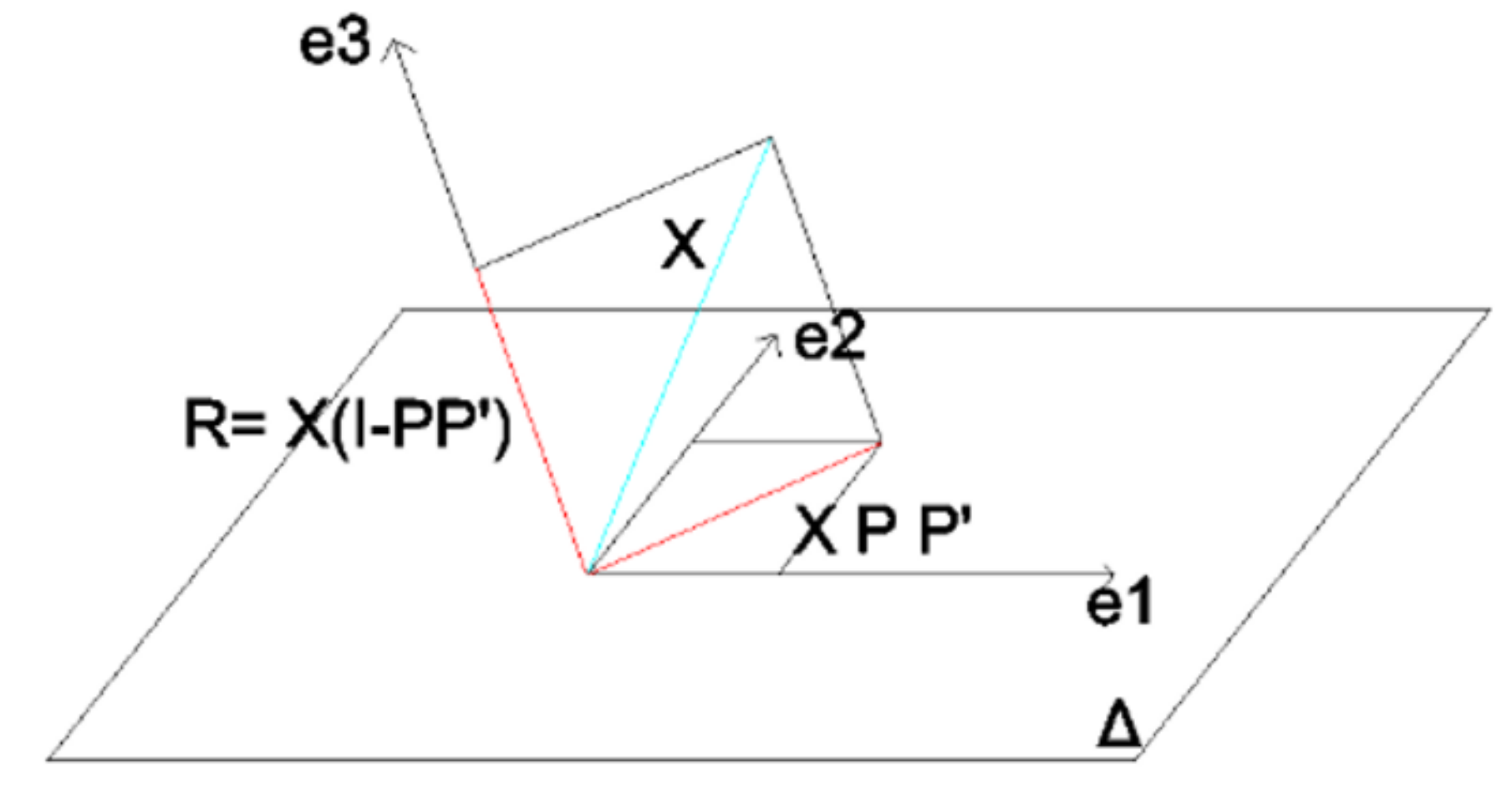
Formulas (5) and (6) have a geometric interpretation. The first step is to define the space made by the r first eigenvector of the matrix X′X. In Figure 1, this space is the plan Δ. The second step is to compute the projection (XPP′, red lines in Figure 1) of the matrix X in the space (Δ) defined previously. These steps are repeated for r = 1, 2, … (one principal component, two principal components, …) in order to obtain a graph with the estimator values versus PC number used.
Finally, T2 is the squared of the vector norm of the projection in the plan weighted by the inverse of the eigenvalue. The T2 values are calculated for each subspace r = 1, 2, 3, … (One principal component, two principal components …).
Q is the square of the norm of the residual vector (R). R is the subtraction between the data vector and its projection in the space made by the r first eigenvector (the subtraction between the vectors X and XPP′). The Q values are calculated for each subspace r = 1, 2, 3, … (One principal component, two principal components …).
In practice, the X matrix is composed of all the modal frequencies (in rows) obtained for each temperature test (in columns). Appling PCA to the X matrix, the eigenvectors and eigenvalues are obtained. P matrix is made with only the r first PC eigenvectors choose. For each dimension of the space (r) a P matrix and, Q and T2 estimator values are obtained. Where r varies from 1 to the maximum number of eigenvectors.
2.3. The Scaled Structure and the Experimental Setup
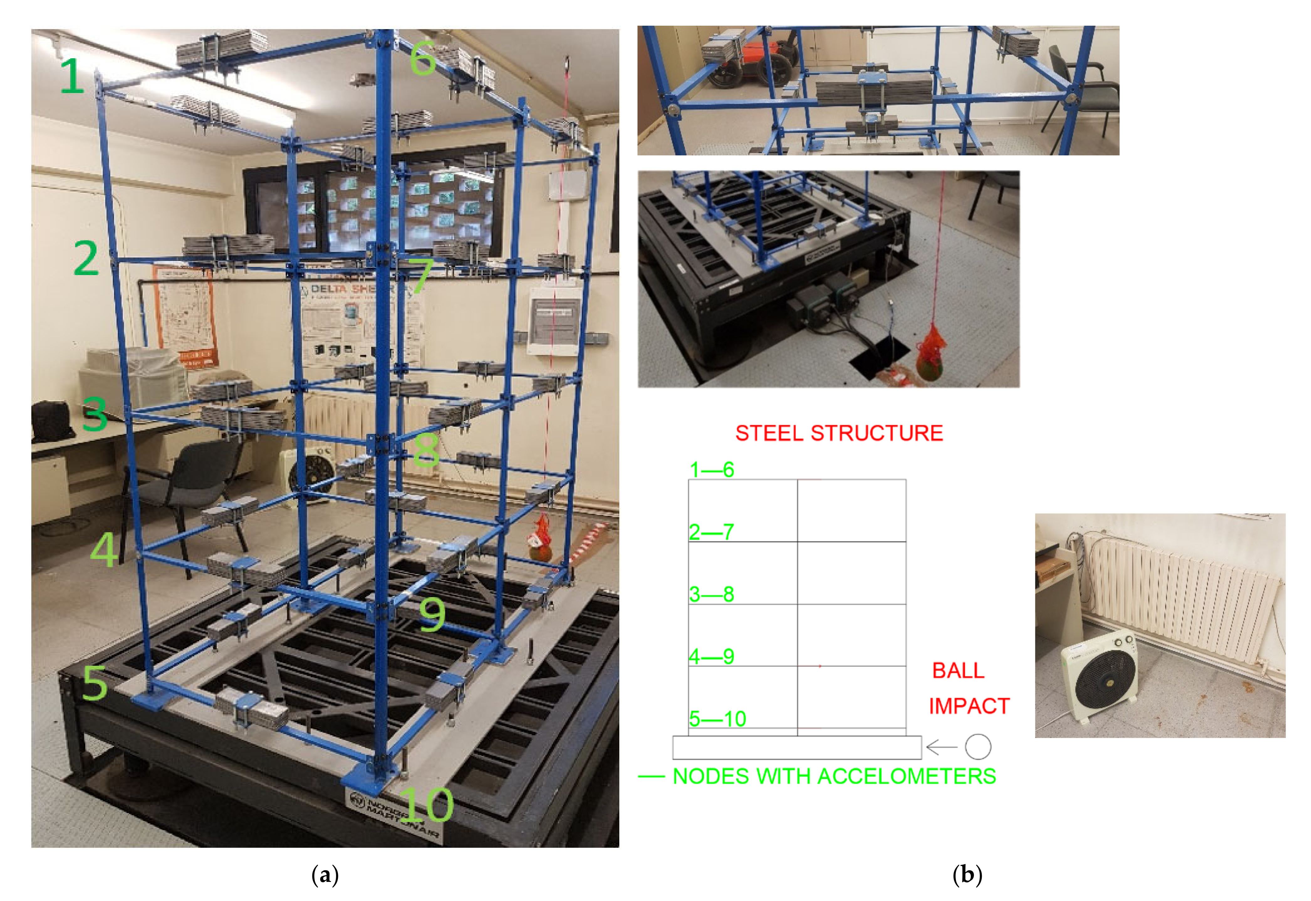
A reduced steel model structure has been used to apply a set of different experimental tests, which are aimed at studying the behavior of the modal frequencies under thermal ambient variations. The scaled steel structure has been modified so that the undamaged and different damaged configurations have been considered in the experimental tests. Numerical models representing the damaged and undamaged structure configurations have been designed and calibrated to complement the experimental tests. The structural model consists of six columns and 35 beams made of steel (Figure 2a). The columns are continuous L shaped 20 mm × 20 mm × 2 mm profiles, and the beams are 20 × 10 mm rectangular shaped bars. The length of each beam is approximately 72 cm for the two-bay frames, and 77 cm for the one-bay ones. Approximately 4.5 kg of lead weight was added in the middle of each beam representing the permanent loads. These added loads consisted of eight 200 mm × 50 mm × 3 mm lead thick plates connected to the model with a steel plate and four bolts.
In order to obtain an adequate excitation of the scaled model, a dense medicinal ball is used to hit the base of the structure. The resulting excitation is obtained under different thermal conditions. The temperature has been controlled by using monitored heaters, which are able to increase the ambient temperature to 30.6 °C. For lowering the temperature until 19.0 °C, an air-conditioning system was used.
The test consists of exciting the structure by hitting its base at different ambient temperatures in the laboratory. Therefore, after finishing each test, the temperature is increased or decreased and a new test is undertaken. The objective was to monitor the structure by repeating the test but at different ambient temperatures. As commented above, the test is performed by using a 2 kg ball and hitting the base of the structure (Figure 2b). The kinematic response of the structure is therefore analyzed by recording, with a set of accelerometers, the acceleration time history of the nodes (Figure 3a,b). The impact force and its corresponding momentum are homogeneous for all the tests because the ball is raised to the same height in each test. Regarding the emulation of the damage conditions of the structure, the impact procedure is performed for five different structure conditions. A first test is performed on the undamaged structure, and four additional tests are undertaken on the structure modified with different damaged configurations. As described above, for each damaged configuration, a range of different ambient temperatures is applied. Then the acceleration is monitored on some specific nodes. The test procedure consists of hitting the structure once every minute. Ten tests were applied successively for each fixed ambient temperature. During the laboratory experiments, the temperature is controlled with a thermometer. However, in order to measure the actual temperature of the structure, a thermographic image was taken by an infrared camera. The joints (Figure 3a) are two vertically positioned bolts at the ends of the beams.
2.4. Monitoring the Frequency Variation under Temperature Control
The experimental setup involves 12 Brüel & Kjaer accelerometers (model 4371) placed in the nodes located in positions 1 to 6 (Figure 2b and Figure 3b). In Figure 3b, the two directions of the accelerometer are detailed in each monitored node with red and blue arrows. The direction of the arrow indicates a positive direction. Accelerometers in positions 1, 4, 8, 10 and 12 were placed in the longitudinal direction (X), while in the transverse direction (Y), the accelerometers were located in positions 2, 3, 5, 7, 9 and 11 (Figure 3b).
The frequency variation was studied by modifying the structure in order to generate five different damaged configurations. So, an initial undamaged configuration, where the end nodes of the beams are considered as fixed; and four damaged configurations obtained by relaxing the bolts located at the nodes of the beams (four different pattern maps of relaxed bolts where used). The following tests were performed:
Test 1: Structure without damage. In this test, all the bolts of the structure were tightened with the maximum torque (5.1 Nm).
Test 2: Medium damage in two nodes. In this test, the structure has a damage in the connections of the nodes in positions 3 and 8, in the longitudinal and transversal beam of the third floor. In this test, the bolts in connections 3 and 8 were relaxed until a torque of 2.5 Nm was reached.
Test 3: High damage in two nodes. In this test, the structure has damage in the connections of the nodes in positions 3 and 8, in the longitudinal and transversal beam of the third floor. In this test, the bolts in the connections 3 and 8 were released (Torque 0 Nm).
Test 4: High damage in three nodes. In this test, the structure has damage in the connections of the nodes in positions 3, 8 and 2, in the longitudinal and transversal beam of the third and fourth floors. In this test, the bolts in the connections 3, 8 and 2 were released (Torque 0 Nm).
Test 5: High damage in four nodes. In this test, the structure has a damage in the connections of the nodes in positions 3, 8, 2 and 7 in the longitudinal and transversal beam of the third and fourth floors. In this test, the bolts in the connections 3, 8, 2 and 7 were released (Torque 0 Nm).
The PCA is properly applied with a minimum number of data that have enough rank variation of the variables. To ensure this procedure, it is necessary to have a minimum number of experiments and a range of temperatures, which are controlled with a thermal camera [16].
For each monitored damaged configuration, the temperature was measured by a thermal camera (Figure 4a). The post-process signal treatment and analysis were carried out with the Infrec Analyser program. For each test, the temperature is controlled with the help of electric stoves, in the case of increasing the heat, and to lower the temperature with the help of an air conditioning device, as commented above. Table 1 shows the temperature range applied in the five tests.
Figure 4a shows the image obtained with the thermal camera for test 1 at 20.5 °C. The colored picture indicates a heterogeneous distribution of the temperature. The upper part of the structure reached a higher temperature while the bottom of the structure remained cooler. For all tests, the same point is used to measure the temperature (highlighted circle in Figure 4a) and is located at the intermediate height of the structure.
3. Results
This section presents the results of the frequency variation with temperature. The authors developed the software for the treatment and post process of the accelerometer records. The autospectra were obtained by averaging 10 windows of each channel and each test. The two last graphics included in Figure 4b shows the channel 1 and 2 energy spectral density (ESD) of the test 1 (undamaged configuration) with 20.5 °C (performed 24 July 2019). In these two graphics, the peaks of the second mode (2.703 Hz) are signposted. The ESD for this mode in the first channel is 2.506·105 m2/s/Hz and 5.048·103 m2/s/Hz for the second channel. The second graphic shows the coherence between the two channels. For the peak (mode 2) related to the 2.703 Hz frequency, the calculated coherence is 0.9955, which indicates a good linear dependency between both channels. Consequently, this indicates that the peak is generated by the same effect. Finally, the first graphic in Figure 4b is the phase of the cross spectrum. For the second mode, the second channel has a phase lag of −3.066 rad when compared to the first one. Therefore, both channels are in opposite signs.
In longitudinal accelerometers, higher modes present a non-symmetric peak related with a non-linear behavior (red circle in Figure 4b).
3.1. Peak Picking: Frequency Patterns
The ESD of the different experiments presents a similar pattern. In the spectrum, the peaks are selected to create the matrix X for each test where the PCA theory is applied. In our study, 13 modal frequencies have been correctly detected by the peak picking method for all damaged and undamaged configurations. Table 2 shows the frequencies for only the ten first modes and the 13 temperature tests for the undamaged configuration of the structure. Only the first 13 modal frequencies were chosen because the upper frequencies show clear non-linear behavior. For each damaged test, the selected modal frequencies are ordered in the same way for all temperature tests. In the matrix X, each column corresponds to the frequency modes from 1 to 13 and each row correspond to tests with different temperatures.
In ESD, the frequency peak patterns are similar between channel 1 and 2 for modes 2 to 13. However, mode 1 only appears in the longitudinal channel (Figure 4b). It is also important to highlight that, for the tests performed on high damaged configurations and for all the temperatures in the range of study, the first mode, which is orthogonal to the direction in which the structure is excited, was not clearly detected and, consequently, it has not been used in the PC analyses.
Table 3 presents the frequency decay of the damaged tests (test 2, 3, 4 and 5) when comparing to the results with the undamaged configuration (test 1).
The standard deviation of the modal frequencies in the undamaged configuration test is lower than 0.016 Hz for the first six modes, and lower than 0.05 Hz for upper modes, while the frequency resolution is 0.016 Hz. Moreover, the standard deviations of the measured frequencies in test 2 (medium damaged configuration) are lower than the resolution (0.016 Hz) for the first six modes and the 10th and 13th modes, and they are lower than those obtained for the undamaged configuration of test 1 (21% lower on average). In the case of test 3 (high damage in two nodes), the standard deviations are lower than 0.016 Hz for the first six modes and for the 10th mode, and lower than the standard deviation obtained in the undamaged configuration test 1 (98% lower on average). In the case of high damage in three nodes (test 4), the standard deviations are lower than the frequency resolution for the first six modes and for the 10th mode, and they are slightly lower (6.73% lower on average) than those obtained in the undamaged configuration test. Finally, the standard deviation of the frequency data for test 5 (high damage in four nodes) is greater than the resolution frequency in almost all modes (only the first and fourth modes have lower standard deviations). In this test, the average of the standard deviation is higher than that obtained in the undamaged configuration tests (276%).
3.2. The Variance Explanined Results
The variance explained is studied for all the damaged configuration tests. Each principal component is associated to a percentage of variance explained. Figure 5 represents the cumulative variance explained vs. the number of principal components used for each of the damaged tests.
The test that has the highest cumulative variance explained for almost all the principal component numbers chosen is the high damaged configuration test 3 (damage in two nodes). The test that has the lower explained cumulative variance is the high damaged configuration test 4 (damage in three nodes). For the undamaged configuration test, three principal components are enough to explain 95% of the data variance and have a flat curve slope. The medium damaged configuration test 2 (damage in two nodes) also needs three principal components before the change of the curve slope in order to explain 95.5% of the total variance. Test 3 (high damage in two nodes) and test 5 (high damage in four nodes) also needed three principal components in order to explain 98% of the data variance. Test 4 (high damage in three nodes), the only damage configuration that includes an asymmetric damage distribution pattern, needed four principal components to make the cumulative variance curve flat and explain 97% of the variance of its data.
To properly apply the proposed methodology, enough of a temperature range is needed in order to assure the frequency variations are higher than the frequency resolution. Otherwise, the variance obtained by PC analysis mainly reflects the random error produced by the lack of resolution.
The evolution of the principal components with the temperature for the undamaged configuration test shows a minimum of 9 degrees of temperature range to assure the stability of the cumulative explained variance of the PC (Figure 6). Similar results occur in the other tests.
3.3. Q Results
For each damaged configuration test, the Q value is computed as explained in Section 2.2 Equation (6). Figure 7 shows the results of Q values vs. principal component number related to the damaged configuration tests performed in this study.
The undamaged configuration test (test 1) shows the lower Q values for all the principal component number, while the test with higher Q values, is the high damaged configuration test 5 (damage in four nodes).
The Q values derived from the tests are ordered according to the increasing damage level (Figure 7a). The Q values in the undamaged and medium damaged configurations (tests 1 and 2) are smaller than those calculated for the high damage configuration structures (tests 3, 4 and 5). The Q values of the high damaged configuration test 5 (damage in four nodes) are higher than those of the high damage configuration test 4 (damage in three nodes). In addition, the Q values of the high damage configuration test 4 (damage in three nodes) are bigger than the high damage configuration test 3 (damage in two nodes).
In tests 3, 4 and 5 (structures with high damaged configurations), the Q values increase monotonically after the fifth principal component. The fifth principal component is the inflexion point (Figure 7a). However, for the tests 1 and 2 (undamaged and medium damaged structures), Q values increase monotonically since the first principal component. Therefore, in these two cases, only one principal component is needed to reach the inflexion point (Figure 7a).
Although tests 1 and 2 do not indicate a significant shape difference (Figure 7a), when increasing the resolution of the graphic in Figure 7b, it is evidenced that Q values in the undamaged configuration structure (test 1) are smaller than the medium damaged configuration structure (test 2). Not only the Q values are sensitive enough to evaluate the difference between the high damaged, medium damaged and undamaged tests, but it can also differentiate the medium damage configuration (damage in two nodes) from the undamaged configuration structure.
For all the performed tests, when the principal components increase, the Q values decrease, because when the space projection is bigger, the projection is a better approximation of X, therefore, the residual vector is smaller.
3.4. T2 Results
For each of the damaged tests, the T2 value is computed as explained in Section 2.2 Equation (5). Figure 8 shows the T2 values graphic vs. principal component number for each of the damages.
For all the tests, when the number of principal component increases, the T2 values also increase, because when the projection space is bigger, the projection is a better approximation of X. The shape of the T2 graphic has an opposite shape from the Q graphics.
The T2 values of the tests are arranged in increasing order of damage (Figure 8a). The T2 values in the undamaged and medium damaged structures (tests 1 and 2) are smaller than the three high damaged structures (tests 3, 4 and 5). The T2 values of the high damage four nodes structure (test 5) are bigger than the high damage in three nodes structure (test 4). In addition, the T2 values of the three nodes high damage structure (test 4) are bigger than the two nodes high damage structure (test 3).
In tests 3, 4 and 5 (high damaged structure), the T2 values increase monotonically after the fifth principal component. The fifth principal component is the inflexion point (Figure 8a). However, for the tests 1 and 2 (undamaged and medium damaged structure), the T2 values increase monotonically since the first principal component. Thus, in these two cases, only one principal component is needed to reach the inflexion point (Figure 8a).
When increasing the resolution of the graphic (Figure 8b), it can be observed that T2 values in the undamaged structure (test 1) are bigger than those obtained for the medium damaged structure (test 2).
4. Conclusions
Although the variability of the modal frequencies has not been great enough compared with the resolution error, Q and T2 estimators seem to be more sensitive than the cumulative standard deviation. The results obtained in this study point out the importance of ensuring enough frequency variation to have good results. The results show the importance of studying the stability of the cumulative variance explained. There are two ways to increase the variance stability: increase the range of temperature or increase the resolution.
Although the estimator of the variance explained is not entirely conclusive, the T2 and Q estimators point out that the high damaged structures (tests 3, 4 and 5) need 5 principal components to explain the modal frequency variation with temperature. However, the undamaged and the medium damaged structures (tests 1 and 2) only need one principal component.
The Q estimator is arranged according to the damage intensity (Figure 7a). The Q estimator is sensitive enough to establish that values in the undamaged structure (test 1) are smaller than those calculated in the medium damaged structures (test 2).
The T2 estimator is sorted according to the intensity of the damage (Figure 8a). However, the T2 estimator seems not to be sensitive enough because T2 values in the undamaged structure (test 1) are bigger than the medium damaged structure values (test 2). The main causes that may explain these results are the reduced resolution and the short range of temperatures.
The results indicate that the behavior of these estimators could be useful to detect damage and to distinguish among a range of intensities of damage in structures with different configurations. Moreover, it seems to be possible to predict a high damaged configuration by only knowing the minimum number of the principal component of the Q and the T2 to explain the modal frequency variation.
Author Contributions
Conceptualization, O.C., A.M., J.C.; Experimental test A.M., J.C.; Software, O.C., A.M.; Methodology, O.C., A.M.; Formal analysis, O.C., A.M.; Writing, O.C., A.M., Y.F.V.-A., R.G.-D.; Review and editing, O.C., A.M. All authors have read and agreed to the published version of the manuscript.
Funding
This research has been partially funded by the Spanish Research Agency (AEI) of the Spanish Ministry of Science and Innovation (MICIN) through project with reference: PID2020-117374RB-I00/AEI/10.13039/501100011033.
Informed Consent Statement
Not applicable.
Conflicts of Interest
The authors declare no conflict of interest.
References
- Icomos–Iscarsah Committee. ICOMOS charter-principles for the analysis, conservation and structural restoration of architectural heritage. In Proceedings of the ICOMOS 14th General Assembly, Victoria Falls, Zimbabwe, 27–31 October 2003. [Google Scholar]
- Caselles, O.; Martínes, G.; Clapés, J.; Roca, P.; Pérez-Gracia, V. Application of Particle Motion Technique to Structural Modal Identification of Heritage Buildings. Int. J. Archit. Herit. Conserv. Anal. Restor. 2015, 9, 310–323. [Google Scholar] [CrossRef] [Green Version]
- Elyamani, A.; Caselles, O.; Roca, P.; Clapes, J. Dynamic investigation of a large historical cathedral. Struct. Control. Health Monit. 2017, 24, e1885. [Google Scholar] [CrossRef] [Green Version]
- Ivorra, S.; Cervera, J.R. Analysis of the dynamic actions when bells are swinging on the bell tower of Bonrepos i Mirambell Church (Valencia, Spain). In Proceedings of the 3rd International Seminar of Historical Constructions, University of Minho Guimarães, Braga, Portugal, 7–9 November 2001. [Google Scholar]
- Beconci, M.L.; Bennati, S.; Salvatorre, W. Structural characterization of a medieval bell tower: First historical, experimental and numerical investigations. In Historical Constructions; Lourenço, P.B., Roca, P., Eds.; Semantic Scholar: Guimarães, Portugal, 2001; pp. 431–444. [Google Scholar]
- Ramos, L.F.; Marques, L.; Lourenço, P.B.; De Roeck, G.; Campos-Costa, A.; Roque, J. Monitoring historical masonry structures with operational modal analysis: Two case studies. Mech. Syst. Signal Process. 2010, 24, 1291–1305. [Google Scholar] [CrossRef] [Green Version]
- Caselles, O.; Clapes, J.; Sáez Sagasta, J.I.; Pérez-Gracia, V.; Rodríguez Santana, C.G. Integrated GPR and Laser Vibration Surveys to Preserve Prehistorical Painted Caves: Cueva Pintada Case Study. Int. J. Archit. Herit. Conserv. Anal. Restor. 2021, 15, 669–677. [Google Scholar] [CrossRef]
- Santos-Assunçao, S.; Pérez-Gracia, V.; Caselles, O.; Clapes, J.; Salinas, V. Assessment of Complex Masonry Structures with GPR Compared to Other Non-Destructive Testing Studies. Remote Sens. 2014, 6, 8220–8237. [Google Scholar] [CrossRef] [Green Version]
- Perez-Gracia, V.; Santos- Assunçao, S.; Caselles, O.; Clapes, J.; Sossa, V. Combining ground penetrating radar and seismic surveys in the assessment of cultural heritage buildings: The study of roofs, columns, and ground of the gothic church Santa Maria del Mar, in Barcelona (Spain). Struct. Control. Health Monit. 2019, 26, e2327. [Google Scholar] [CrossRef]
- Smith, L.I. A tutorial on Principal Components Analysis; Technical Report OUCS-2002-12; University of Otago: Dunedin, New Zealand, 2002. [Google Scholar]
- Tibaduiza, D.A.; Mujica, L.E.; Rodellar, J. Damage classification in structural health monitoring using principal component analysis and self-organizing maps. Struct. Control. Health Monit. 2013, 20, 1303–1316. [Google Scholar] [CrossRef]
- Golinval, J.C. Damage detection in structures based on principal component analysis of forced harmonic responses. Procedia Eng. 2017, 199, 1912–1918. [Google Scholar] [CrossRef]
- Moropoulou, A.; Polikreti, K. Principal Component Analysis in monument conservation: Three application examples. J. Cult. Herit. 2009, 10, 73–81. [Google Scholar] [CrossRef]
- Yan, A.M.; Kerschen, G.; De Boe, P.; Golinval, J.C. Structural damage diagnosis under varying environmental conditions—Part I: A linear analysis. Mech. Syst. Signal Process. 2005, 19, 847–864. [Google Scholar] [CrossRef]
- Grande, C.J. Correlation between weather Conditions, Heating of Structural Elements, and the Dynamic Behavior of Mallorca Cathedral. Master’s Thesis, Universitat Politècnica de Catalunya, Barcelona, Spain, 2013. [Google Scholar]
- Caselles, O.; Clapes, J.; Elyamani, A.; Lana, X.; Seguí, C.; Martín, A.; Roca, P. Damage Detection using principal component analysis applied to temporal variation of natural frequencies. In Proceedings of the 16ECEE, Thessaloniki, Greece, 18–21 June 2018. [Google Scholar]
- Mujica, L.E.; Rodellar, J.; Fernandez, A.; Güemes, A. Q-statistic and t2-statistic pca-based for damage assessment in structures. Struct. Health Monit. 2010, 10, 1–15. [Google Scholar] [CrossRef]
- Nguyen, V.H.; Mahowald, J.; Golinval, J.C.; Maas, S. Damage detection in civil engineering structure considering temperature effect. In Dynamics of Civil Structures, Volume 4; Springer: Cham, Switzerland, 2014; pp. 187–196. [Google Scholar]
- Zhang, G.; Tang, L.; Liu, Z.; Zhou, L.; Liu, Y.; Jiang, Z.; Sun, S. Enhanced features in principal component analysis with spatial and temporal windows for damage identification. Inverse Probl. Sci. Eng. 2021, 29, 2877–2894. [Google Scholar] [CrossRef]
Figure 1.
Geometric interpretation of Principal Component Analysis.

Figure 2.
(a) Scaled steel model structure with the number nodes (green); (b)The added load, the ball, schema representing the structure, the monitored nodes (green), and the heaters.
Figure 2.
(a) Scaled steel model structure with the number nodes (green); (b)The added load, the ball, schema representing the structure, the monitored nodes (green), and the heaters.

Figure 3.
The scaled model and the experimental setup (a) Longitudinal (blue circle) and transversal (red circle) distribution of accelerometer; (b) Location of the nodes (green) and the accelerometers (red and blue).
Figure 3.
The scaled model and the experimental setup (a) Longitudinal (blue circle) and transversal (red circle) distribution of accelerometer; (b) Location of the nodes (green) and the accelerometers (red and blue).

Figure 4.
(a) Thermal image of the scaled structure for test 1 at 20.5 °C; (b) Phase, Coherence and ESD of Channels 1 and 2 for test 1 at 20.5 °C between 0 and 18 Hz.
Figure 4.
(a) Thermal image of the scaled structure for test 1 at 20.5 °C; (b) Phase, Coherence and ESD of Channels 1 and 2 for test 1 at 20.5 °C between 0 and 18 Hz.

Figure 5.
Cumulative explained variance (%) vs. principal component number.

Figure 6.
Thermal variation of the cumulative variance for the first four principal components used for the undamaged configuration test.
Figure 6.
Thermal variation of the cumulative variance for the first four principal components used for the undamaged configuration test.

Figure 7.
(a) Q values vs. principal component number for all damaged tests. (b) Q values vs. principal component number for tests 1 and 2.
Figure 7.
(a) Q values vs. principal component number for all damaged tests. (b) Q values vs. principal component number for tests 1 and 2.

Figure 8.
(a) T2 values vs. principal component number for all damaged tests. (b) T2 values vs. principal component number for tests 1 and 2.
Figure 8.
(a) T2 values vs. principal component number for all damaged tests. (b) T2 values vs. principal component number for tests 1 and 2.


Table 1.
Temperatures applied in the five tests.
| Temperature (°C) | |
|---|---|
| TEST 1 | 20.5 to 30.6 |
| TEST 2 | 19.4 to 29.5 |
| TEST 3 | 19.9 to 29.9 |
| TEST 4 | 19.0 to 28.5 |
| TEST 5 | 19.2 to 29.1 |
Table 2.
First ten modal frequencies for the undamaged test in the thirteen different temperature tests.
Table 2.
First ten modal frequencies for the undamaged test in the thirteen different temperature tests.
| Frequencies (Hz) | ||||||||||
|---|---|---|---|---|---|---|---|---|---|---|
| Test | Mode 1 | Mode 2 | Mode 3 | Mode 4 | Mode 5 | Mode 6 | Mode 7 | Mode 8 | Mode 9 | Mode 10 |
| 1 | 2.641 | 2.703 | 3.781 | 7.672 | 9.281 | 9.609 | 12.14 | 13.33 | 15.22 | 17.67 |
| 2 | 2.641 | 2.687 | 3.781 | 7.687 | 9.281 | 9.609 | 12.09 | 13.34 | 15.25 | 17.67 |
| 3 | 2.656 | 2.703 | 3.797 | 7.687 | 9.281 | 9.625 | 12.17 | 13.36 | 15.28 | 17.69 |
| 4 | 2.656 | 2.703 | 3.797 | 7.703 | 9.281 | 9.625 | 12.19 | 13.36 | 15.28 | 17.70 |
| 5 | 2.641 | 2.703 | 3.797 | 7.703 | 9.281 | 9.625 | 12.17 | 13.37 | 15.27 | 17.70 |
| 6 | 2.656 | 2.703 | 3.797 | 7.703 | 9.297 | 9.640 | 12.22 | 13.37 | 15.31 | 17.72 |
| 7 | 2.656 | 2.703 | 3.797 | 7.703 | 9.297 | 9.640 | 12.19 | 13.36 | 15.23 | 17.70 |
| 8 | 2.656 | 2.703 | 3.797 | 7.703 | 9.297 | 9.640 | 12.22 | 13.36 | 15.27 | 17.72 |
| 9 | 2.656 | 2.703 | 3.797 | 7.687 | 9.297 | 9.640 | 12.20 | 13.3 | 15.27 | 17.72 |
| 10 | 2.656 | 2.703 | 3.797 | 7.687 | 9.297 | 9.640 | 12.22 | 13.3 | 15.27 | 17.70 |
| 11 | 2.656 | 2.703 | 3.797 | 7.672 | 9.297 | 9.640 | 12.20 | 13.28 | 15.25 | 17.72 |
| 12 | 2.656 | 2.703 | 3.797 | 7.672 | 9.297 | 9.640 | 12.23 | 13.27 | 15.27 | 17.72 |
| 13 | 2.656 | 2.703 | 3.797 | 7.672 | 9.297 | 9.640 | 12.22 | 13.27 | 15.31 | 17.72 |
Table 3.
Frequency decay of damaged tests when comparing with the undamaged configurations test.
| Frequency Decay (%) | |
|---|---|
| TEST 2 | ≤0.1 |
| TEST 3 | 0.5 to 5 |
| TEST 4 | 1.7 to 7 |
| TEST 5 | 2.6 to 10.3 |
Publisher’s Note: MDPI stays neutral with regard to jurisdictional claims in published maps and institutional affiliations. |
© 2022 by the authors. Licensee MDPI, Basel, Switzerland. This article is an open access article distributed under the terms and conditions of the Creative Commons Attribution (CC BY) license (https://creativecommons.org/licenses/by/4.0/).
Share and Cite
MDPI and ACS Style
Caselles, O.; Martín, A.; Vargas-Alzate, Y.F.; Gonzalez-Drigo, R.; Clapés, J. Estimators for Structural Damage Detection Using Principal Component Analysis. Heritage 2022, 5, 1805-1818. https://doi.org/10.3390/heritage5030093
AMA Style
Caselles O, Martín A, Vargas-Alzate YF, Gonzalez-Drigo R, Clapés J. Estimators for Structural Damage Detection Using Principal Component Analysis. Heritage. 2022; 5(3):1805-1818. https://doi.org/10.3390/heritage5030093
Chicago/Turabian StyleCaselles, Oriol, Alejo Martín, Yeudy F. Vargas-Alzate, Ramon Gonzalez-Drigo, and Jaume Clapés. 2022. "Estimators for Structural Damage Detection Using Principal Component Analysis" Heritage 5, no. 3: 1805-1818. https://doi.org/10.3390/heritage5030093