
Enhancing Short-Term Berry Yield Prediction for Small Growers Using a Novel Hybrid Machine Learning Model


1
Department of Management and Marketing, University of Huelva, Pza. de la Merced s/n, 21002 Huelva, Spain
2
Agricultural Economics Research Group, University of Huelva, Pza. de la Merced s/n, 21002 Huelva, Spain
*
Author to whom correspondence should be addressed.
Horticulturae 2023, 9(5), 549; https://doi.org/10.3390/horticulturae9050549
Submission received: 4 April 2023
/
Revised: 27 April 2023
/
Accepted: 28 April 2023
/
Published: 3 May 2023
(This article belongs to the Special Issue Advances in Horticultural Economics, Policy, Business Management and Marketing)
Abstract
:This study presents a novel hybrid model that combines two different algorithms to increase the accuracy of short-term berry yield prediction using only previous yield data. The model integrates both autoregressive integrated moving average (ARIMA) with Kalman filter refinement and neural network techniques, specifically support vector regression (SVR), and nonlinear autoregressive (NAR) neural networks, to improve prediction accuracy by correcting the errors generated by the system. In order to enhance the prediction performance of the ARIMA model, an innovative method is introduced that reduces randomness and incorporates only observed variables and system errors into the state-space system. The results indicate that the proposed hybrid models exhibit greater accuracy in predicting weekly production, with a goodness-of-fit value above 0.95 and lower root mean square error (RMSE) and mean absolute error (MAE) values compared with non-hybrid models. The study highlights several implications, including the potential for small growers to use digital strategies that offer crop forecasts to increase sales and promote loyalty in relationships with large food retail chains. Additionally, accurate yield forecasting can help berry growers plan their production schedules and optimize resource use, leading to increased efficiency and profitability. The proposed model may serve as a valuable information source for European food retailers, enabling growers to form strategic alliances with their customers.
1. Introduction
Perishable agricultural products such as fruits and vegetables are highly time-sensitive and require swift and efficient delivery to maintain their freshness and quality. In addition, farmers are the weakest link in the modern food value chain [1], which is made up of complex sequences of operations with strong social, labor, economic, and environmental implications. Hence, the asymmetries in the food value chain have serious consequences for society in general and farmers in particular [2]. For this reason, the rise of digital technologies could help transform agriculture [3], and predictive models would be a viable option for farmers to improve sales channels with food retailers [4].
As a result of intense competition among large food supermarkets, more and more retailers now tend to demand on-time delivery schedules from their suppliers and are less tolerant of any deviations in their supply schedules. Retailers seek to maintain high-quality service without increasing prices, so maintaining profitability is always a challenge. In this context, the emergence of the omnichannel has revolutionized retail operations resulting in fundamental changes in the expectations of consumers and in the decision-making processes of retailers [5,6,7]. In this sense, researchers have recognized that omnichannel is the future of retail [8].
While demand forecasting is crucial in the supply chain, there has been little research on this topic in relation to omnichannel retailing [9]. To synchronize supply and demand in omnichannel retailing, a data-driven approach that utilizes k-means to identify sales patterns from historical data and uses neural networks to provide accurate forecasting through time series analysis has been proposed [10]. Other approaches include demand forecasting through exponential smoothing [11] and the application of different demand functions to replace the forecasting process [12]. To the best of our knowledge, no studies have addressed the issue of supply forecasting for the horticultural industry in omnichannel retailing, except for the research mentioned previously.
Horticultural products, in general, and the berry sector, in particular, involve seasonal production patterns and price instabilities that have been little studied in the literature but are important in commodity markets, not only operationally but also financially [13]. Due to the highly perishable nature of fresh berries and the globalized nature of the market, large-scale food retailers possess significant bargaining power in the global fresh berry industry through their ability to set prices for future weekly sales programs. For farmers, any deviation from the quantities specified in such programs can result in very significant economic losses when the quantity supplied is lower (penalties for non-compliance) or higher (lower sale prices) than the contractually agreed amount.
Because inaccurate production forecasts may lead to penalties as a result of contract overage, yield prediction systems have become fundamental tools for providing berry growers with better means of market planning [14].
In this study, we aimed to enhance the efficiency of fresh fruit and vegetable suppliers’ order-fulfillment processes while enabling retailers to offer prices of perishable produce to customers in advance [2]. With the emergence of advanced analytical techniques, including neural networks and machine learning (ML), there is a significant opportunity for horticultural farmers to improve yield prediction and generate greater revenue by determining the optimal harvest time and integrating this information into their customers’ e-commerce platforms [5,15].
Hence, accurate yield forecasting can be seen as a competitive factor for farmers due to large retailers typically demand consistent and reliable supplies of products to meet the needs of their customers. By producing accurate forecasts, they can enhance their reputation and increase their own bargaining power. This approach also has the potential to solve a key agronomic challenge, as yield prediction is important for many soft fruit growers because they are dealing with perishable, high-value, seasonally produced fruit and, in addition, harvesting depends on increasingly costly labor.
Our empirical study focuses on this market and proposes an improved method for short- and medium-term yield forecasts, building on the recent literature on time series predictive models. The motivation behind our approach is also to develop an accurate predictive algorithm that can efficiently exploit data from a single variable, such as yield, as other inputs, such as imagery, climate, or plant data, can be expensive and challenging for farmers to obtain.
In short, using only previous yield data as input, the main contribution of this work consists of the development of a new hybrid model for berry yield prediction based on statistical models, such as a time series analysis, in combination with ML techniques. A hybrid model typically consists of two or more models that are combined in a specific way to take advantage of their strengths and mitigate their weaknesses. In our study, the hybrid models for predicting yield in agriculture combine an ML algorithm, such as nonlinear autoregressive neural networks (NARs) and support vector regression (SVR), with a new Kalman filter approach. The statistical model identifies and accounts for trends and seasonality, while the ML algorithm helps to capture complex patterns on the time series of the error. To the best of our knowledge, this is the first approach to use this type of hybridization.
In addition, we compared different models, both non-hybrid and hybrid, using metrics such as root mean square error (RMSE), mean absolute error (MAE), and goodness-of-fit R2, to demonstrate the better performance of the hybrid models. To prove this, we analyzed three berry products separately and showed that the hybrid prediction models are valid for all these time series data.
Our results indicate that producers could take advantage of ML techniques to define digital marketing strategies that minimize their risks and improve their competitive position in the food value chain [16].
The paper is structured as follows: First, we review the different types of predictive models that exist in the literature, with emphasis on those recently used in agriculture. Second, we describe time series data and hybrid models. Third, we present the results of both hybrid and non-hybrid models. Finally, in the last two sections, we discuss the results and their implications.
2. Theoretical Background
Time series forecasting is a widely discussed problem, and we applied a novel approach in pursuit of a solution to this problem for perishable fruit and vegetable products.
Among the most commonly used time series predictive models, the auto-regressive integrated moving average (ARIMA) and seasonal auto-regressive moving average (SARIMA) use a linear regression based on the past values of a variable to be estimated, as well as errors previously made by the process. These models have been used for predictions in many areas [17,18,19,20,21,22,23,24,25,26], including the agri-food sector [4,27,28].
The Kalman filter has often been used to refine an ARIMA model by introducing a state-space system [29,30,31,32,33]. Despite the limited explicit references to the Kalman filter in the field of agri-food production [13], recent studies have utilized this technique for fitting predictive models within the horticultural sector [34].
Alongside linear models, several nonlinear algorithms and ML techniques have also been recently developed to predict time series data [15]. These include NAR, a generalization of the ARIMA model with more complex modeling, which has been applied for predicting the price of minerals [35], the price of certain vegetables [36], amounts of waste [37], water levels [38], COVID-19 case numbers [39], and other variables from different areas [40,41]. In addition, for some years now, numerous studies have adapted types of neural networks—especially SVR—to make time-series predictions in such areas as energy [42,43], finance [44,45,46], weather [47,48], water [49,50,51,52,53], COVID-19 [54], and agriculture [55,56,57,58].
Other recent studies have used hybrid prediction models, involving a combination of different methods, to predict future situations, including demand for flights in the aeronautical industry [59]; electrical energy consumption [60]; and in areas such as weather [61], finance [62], and agriculture [63,64,65,66]. In many such cases, the simplest hybrid algorithm has produced the best predictive result [67].
Currently, extensive research is being conducted in the agricultural sector to predict crop yields better using ML algorithms [68,69,70]. The information facilitated by remote sensing allows for the speedy collection of large amounts of data and offers the potential for extracting data from many variables quickly [71]. Most research using ML for yield forecasting has also involved the use of multispectral imagery data from satellites or unmanned aerial vehicles (UAVs) [71,72,73,74,75]. Some of these studies have sought to predict berry yields using ML-based predictive models [76,77,78].
However, the aforementioned studies on prediction in time series also reveal certain limitations in the field of perishable crop yield forecasting. Firstly, although ML has been identified as one of the most common techniques for yield prediction in agriculture [79], it is not always easy for yields to be predicted because ML algorithms require large amounts of data to provide reliable results [80], and this is not typically available from berry farms. For this reason, although big data analysis is becoming increasingly common in the agricultural sector [81], obtaining the amount of data needed for ML implementations remains a challenge. Secondly, the difficulty in developing yield forecasting models is related to the appropriate selection of independent variables [82]. Thirdly, the prediction models do not adequately capture trend changes in instabilities on the dependent variable. Consequently, this type of predictive system, which is based on the past information of the variable, exhibits a very characteristic deviation to the right, as has been demonstrated in a large body of recent research [83,84,85,86,87].
3. Material and Methods
3.1. Description of the Data
More than 50 percent of all Spanish farms are small farms with less than 5 hectares [88]. Such farms face the need to concentrate supply in order to become more competitive. This is especially the case for Spanish berry growers. In this study, we focused specifically on the Huelva area of Spain because this region is the main producer and exporter of fresh berries in Europe [89] and because Huelva berry growers are usually grouped into cooperatives for the distribution of their products [90].
During the summer, berry cooperatives carry out preliminary deals with their clients (retailers and wholesalers) that are formalized in purchase commitments. When the harvest season starts, these agreements are put into effect by means of weekly sales programs in which prices and daily quantities to be supplied by the cooperative are established. Any non-compliance with agreed conditions results in penalties for producers. If the quantity supplied is less than the agreed amount, a financial penalty is applied. If the quantity supplied exceeds the agreed amount, the product is sold to customers at a much lower price.
To demonstrate that our model was fully functional, we fitted it using a berry yield dataset. This dataset contained data for three berry fruits from farms of Huelva (Spain), corresponding to three periods or seasons.
We worked with a daily berry yield dataset containing data for strawberries, raspberries, and blueberries; these data were obtained from 328 small berry growers from four representative agri-food cooperatives. A longer time series was not possible because of the difficulty in obtaining reliable yield data.
In order to ensure that seasonal time periods were equal, September 1st was chosen as the start date, and July 15th of the following year was chosen as the end date for each agricultural season. In total, we obtained a time series involving approximately 1000 observations of each berry fruit, giving a total of 2835 records in the dataset, which we considered sufficient to run our algorithm.
For the training and testing of our model, we used the first two seasons (2017–2018 and 2018–2019) as the training dataset and the last season (2019–2020) as the testing dataset.
3.2. Description of the Hybrid Model
In recent years, ML algorithms have achieved remarkable success in various areas, including agriculture, as described in the theoretical background above. However, the superiority of ML over other simpler algorithms has not been so apparent in the field of forecasting [67], where data availability is often limited, and regressors are not available [91].
Hybrid prediction models strategically combine several algorithms to exploit the particular advantages of different methods, resulting in more accurate estimations compared to other models [92,93]. In this study, we built on previous research [61,94,95,96,97,98] to propose two hybrid forecasting models. The first model uses a novel approach of the Kalman filter [34] combined with a multilayer perceptron (MLP) neural network that has one hidden layer as its base architecture. The second model replaces NAR with SVR.
Thus, our two hybrid models calculated the prediction of the time series with the Alternative Kalman Filter (AKF) and corrected the error-making predictions about the errors that the predictive system will commit, either through a NAR or an SVR process.
Hence, because hybrid models applied to time series forecasting tend to achieve better performance than pure statistical or pure ML methods [67], by considering Xt as the time series that we intended to estimate and at ~ N (0, σ2) as the white noise process associated with the predictive system, the hybrid model can be expressed as in Equation (1):
where is the linear prediction of the AKF on the time series, and is the estimated error deduced by a NAR or SVR process.
The ARIMA process is one of the most widely used models for time series forecasting. It is a regressive process that depends on past values of the variable to be estimated and on any errors made by the process itself. Our algorithm automatically chooses the optimal ARIMA(p, d, q) parameters that minimize both the Akaike information criterion (AIC) and Bayesian information criterion (BIC).
The introduction of an ARIMA model into a state-space system, if it is carried out using the classical method [99,100], causes problems when the standard deviation of the white noise associated with the system is too large because the algorithm requires the introduction of a random value that can distort the result. In order to eliminate this potential problem, in this study, we followed a new method, namely, AKF [34], which eliminates the introduction of a random value generated by the machine and which can be defined by the equation of state (2), as follows:
where Xt is a stationary zero-mean time series; at is a white noise process associated with the ARIMA(p, d, q) process; m = max{p, q}, where p and q are the delays calculated according to Box–Jenkins methodology; and φi, θj ∈ R are the parameters associated with the ARIMA(p, d, q) process, such that φi = 0 if i > p and θj = 0 if j > q.
The observation Equation (3) can now be expressed as follows:
Our predictive system, therefore, applies the Kalman filter [101] to Equations (2) and (3) and thereby solves the above-mentioned convergence problems.
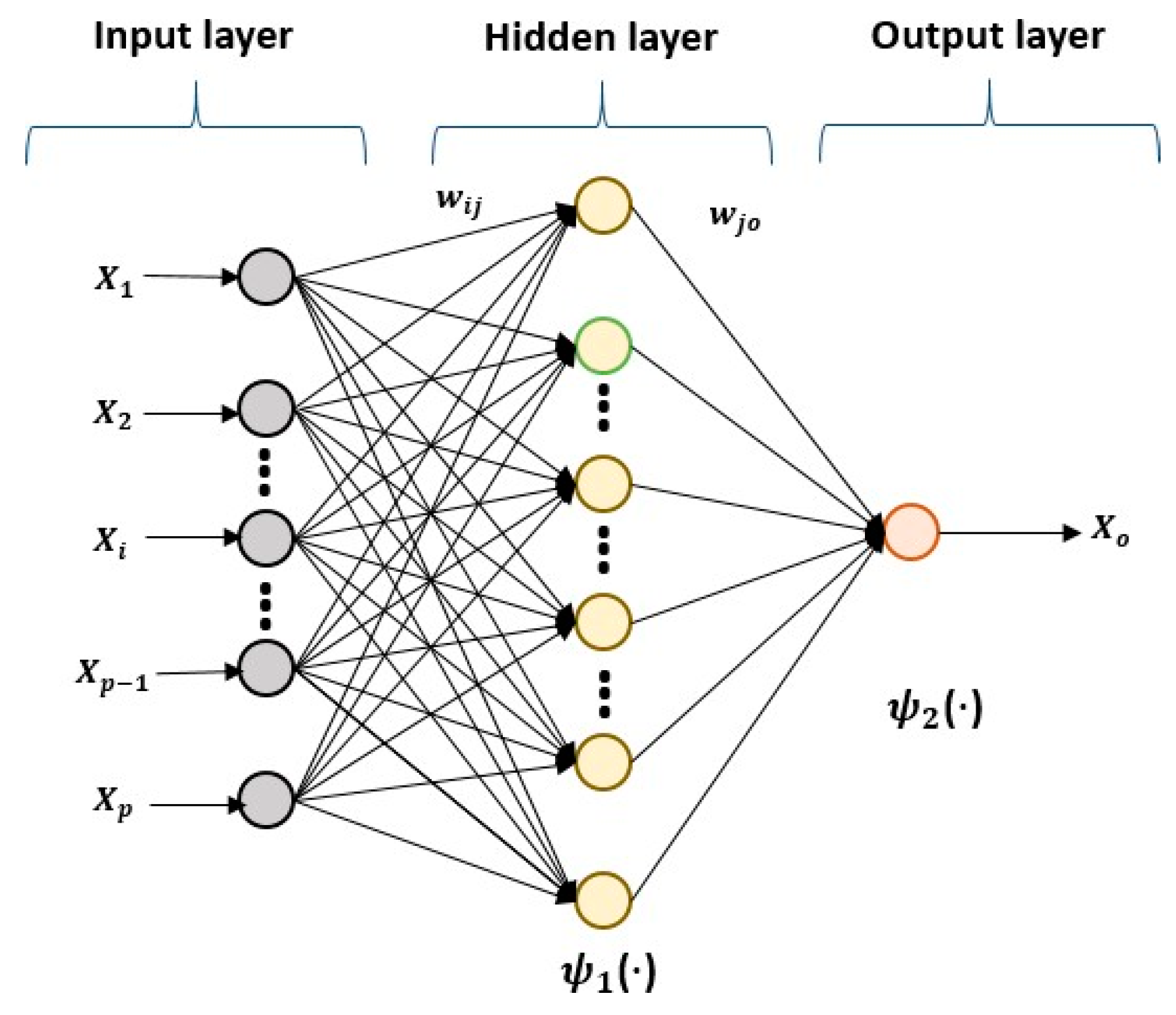
A NAR process is a type of MLP neural network consisting of a nonlinear regression of the variable to be estimated with respect to its own past that can be defined by the expression Xt = f (Xt−1, …, Xt−p) + at, where Xt is the time series, p ∈ N is the number of delays used by the system, at ~ N (0, σ2) is the white noise process of the system, and f is a nonlinear function, generally unknown.
We used the NAR process with a single hidden layer [102], as in Equation (4), as follows:
where ψ1 and ψ2 are the activation functions in the hidden layer and in the output layers, respectively; wij and wj0 are the weights from input i to hidden unit j and from hidden unit j to output o, respectively; and bj and bo are the biases in the corresponding units (Figure 1).
The number of inputs p and the number of units in the hidden layer M were obtained using a growth technique, first in the input layer and then in the hidden layer, adding units step by step and calculating the RMSE on the training set. Finally, p and M were determined when a minimum RMSE value was found.
For the activation functions, we tested the sigmoidal function and the hyperbolic tangent in the hidden layer, choosing the one that obtained the lowest RMSE in the training set, and the identity function in the output layer, as has been previously described for regression problems [37,61,62,103,104].
Finally, as a learning algorithm, we used the backpropagation algorithm, which can correct the weights minimizing the error made in the training set. Therefore, if we consider Wl the weight matrix of layer l = 1, 2, the backpropagation algorithm calculates the increments as follows:
where η ∈ R is the learning rate, and E∗ is the error made by the system in each step of the training. For the learning rate, we used the value in the interval [0.01, 0.1] that minimizes the RMSE in the training set, tested in increments of 0.01.
SVRs are a type of ML derived from the adaptation of SVM used for nonlinear regressions. For calculation purposes, we used Equation (5) as follows:
where k is the kernel function, and (αj − αj*) ≠ 0 values are support vectors.
We made error corrections by the linear system and computed a prediction on the time series of the error, which is a type of white noise variable, using the Gaussian function as the kernel function. Lastly, we chose the number of inputs in a similar way to the method used in the NAR model by increasing the number of lags one by one and observing the RMSE in the training set until we found a minimum through package e1071 of the R programming language to determine the value of the parameters needed for this model.
4. Results
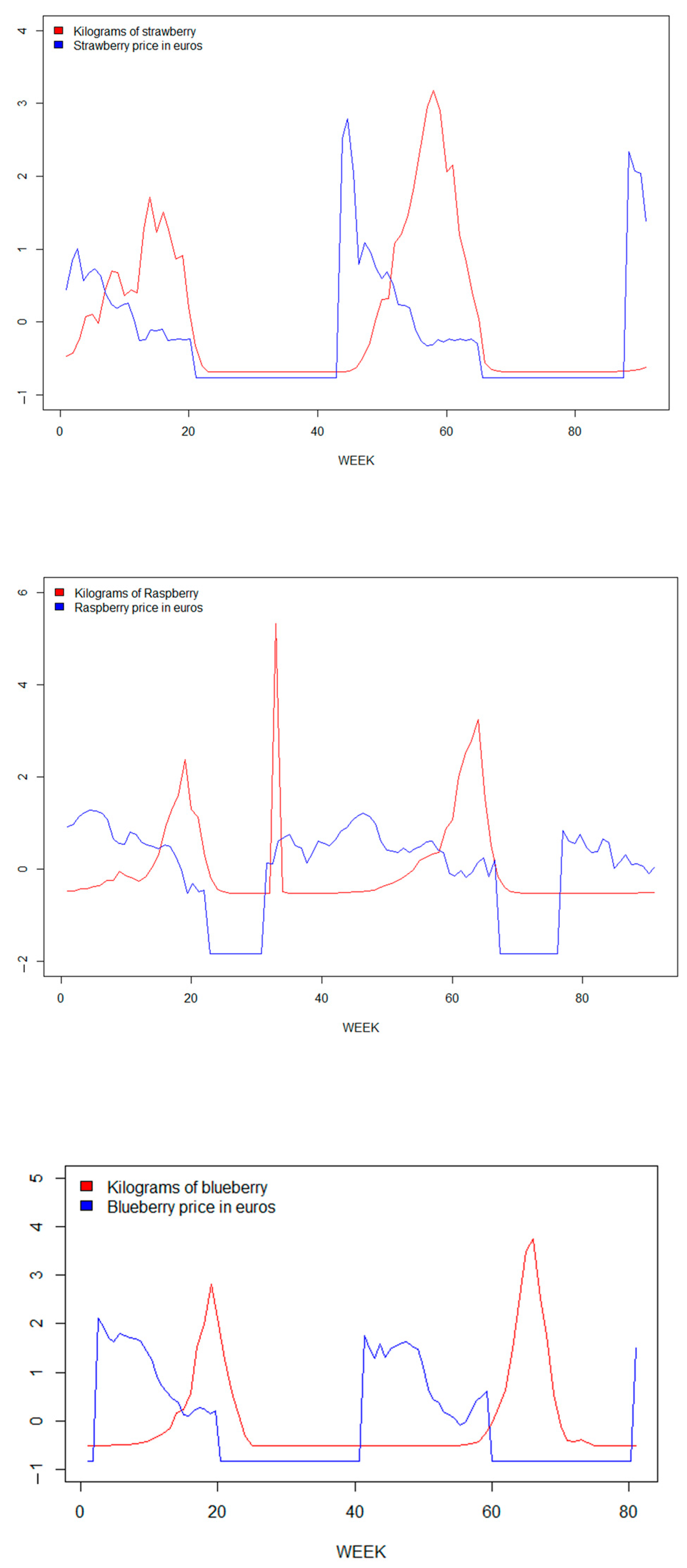
Supply agreements are key contributors to berry farm profitability; however, profit levels for berries ultimately depend not on growers but on retailers. In addition, time series of prices and yields are characterized by temporal variability (Figure 2).
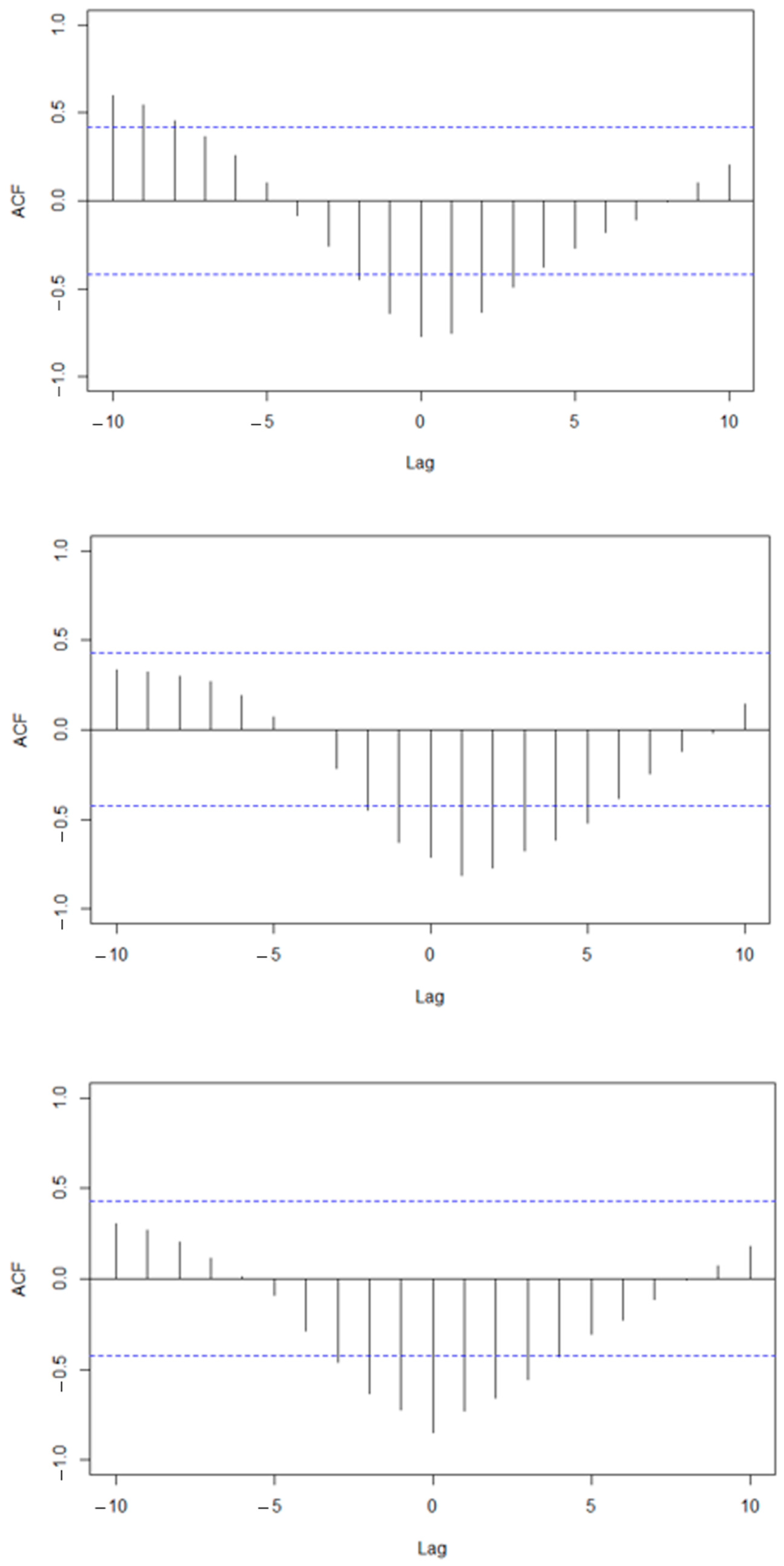
Specifically, we can observe in the cross-correlation functions (Figure 3) that, in all three cases, both time series present a large negative correlation, especially in lag 0 when the value of the linear correlation is greater than −0.7. This adds further value to a predictive system.
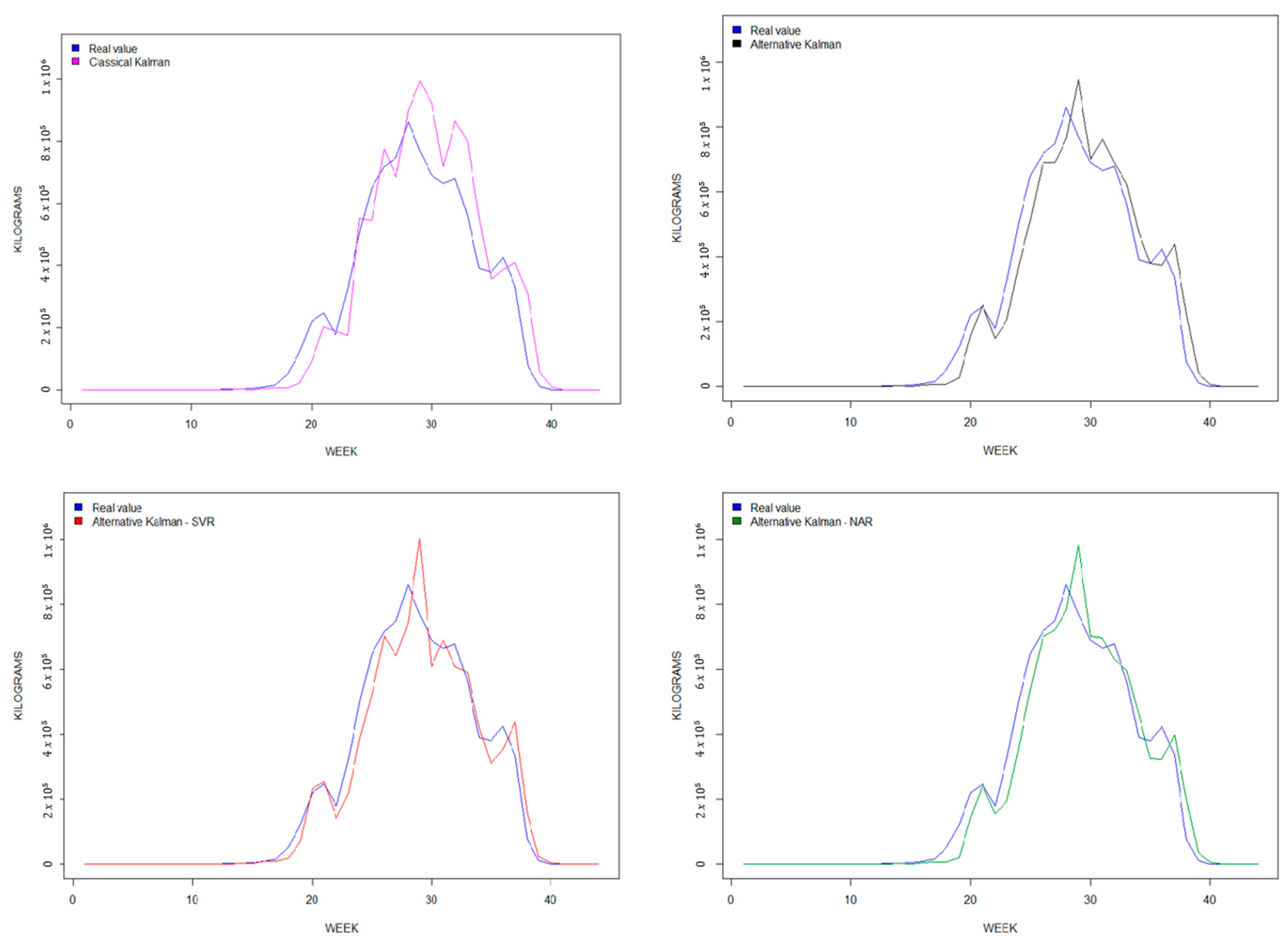
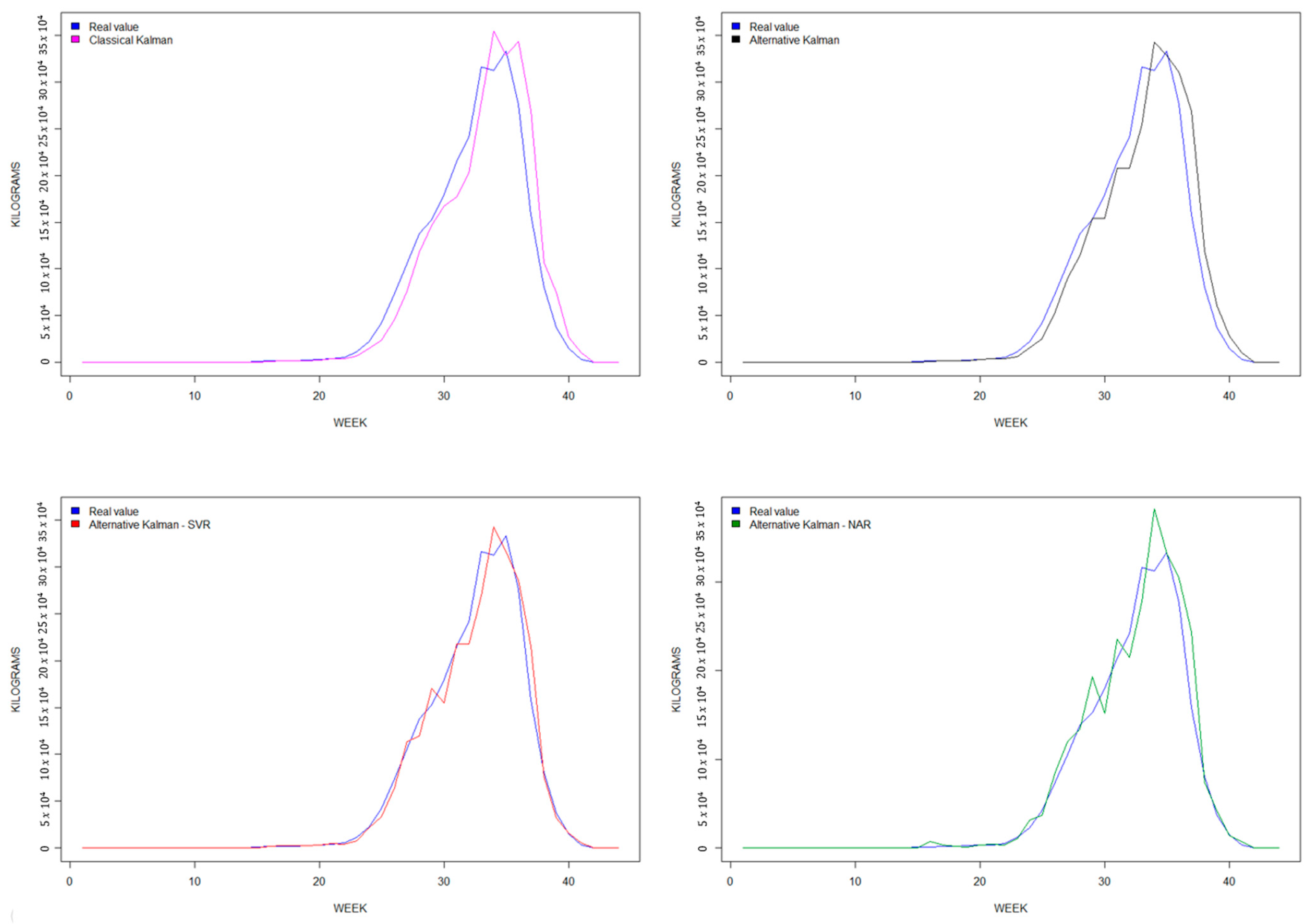
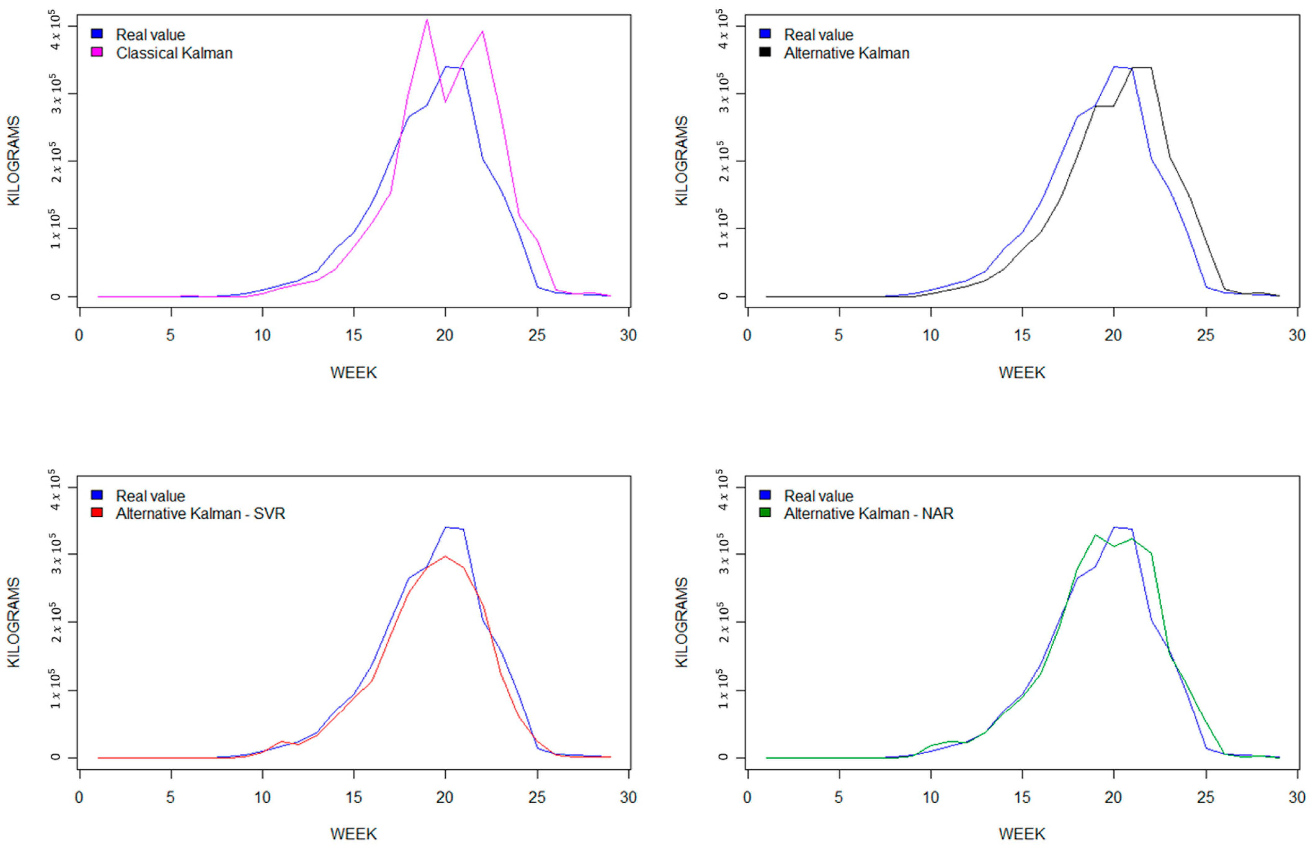
In this section, we analyzed the results obtained for the weekly predictions of three berry crops during the 2019–2020 season and compare the results obtained using (1) the classical Kalman filter-based model and (2) the AKF-based model with those obtained using (3) the hybrid AKF-SVR model and (4) the hybrid AKF-NAR model. The selection of parameters for each model is detailed in Section 3.
We compared the results of the four models using RMSE, MAE, and goodness-of-fit R2 criteria to minimize errors while not penalizing a higher number of parameters, as required in nonlinear processes.
For the weekly strawberry season forecast, our algorithm automatically chose the optimal ARIMA parameters that minimized the AIC and BIC criteria, resulting in the ARIMA(3, 1, 1) model. For the AKF-SVR model, we used a Gaussian kernel function with γ = 0.1, C = 1, and ϵ = 0.1, and eight inputs; for the AKF-NAR model, a hyperbolic tangent activation function in the hidden layer, with η = 0.01, p = 4, and M = 1.
Table 1 summarizes the results for the 2019–2020 season. These indicate that AKF improved upon the classical Kalman filter, and neural network correction further improved performance. Thus, the AKF-SVR and AKF-NAR models were found to be the most accurate.
Similarly, for raspberry, we used an ARIMA(1, 1, 1) model and a Gaussian kernel function with γ = 0.071, C = 1, ϵ = 0.1, and 14 inputs for the AKF-SVR model. For the AKF-NAR model, we used a hyperbolic tangent function as the activation function in the hidden layer, with η = 0.1, p = 16, and M = 1. Again, the hybrid AKF-SVR was the best predictive model, followed closely by the hybrid AKF-NAR (see Table 2).
For blueberry, we used an ARIMA(6, 1, 1) model and a Gaussian kernel function with γ = 0.1, C = 1, and ϵ = 0.1, and 10 inputs, for the AKF-SVR model. For the AKF-NAR model, we used a sigmoid function as the activation function in the hidden layer, with η = 0.1, p = 10, and M = 1. Table 3 shows that the AKF-SVR model was the most accurate in predicting blueberry season values.
Finally, it is worth noting that our two hybrid models exhibit a goodness-of-fit greater than 0.95 across all three data series. These results demonstrate how the predicted yields from the hybrid models align better with the actual yield values compared to the non-hybrid models. To visualize this improvement, Figure 4, Figure 5 and Figure 6 display a comparison of the four predictive models for each berry fruit in terms of the observed real variable, which is the weekly berry yield measured in kilograms.
5. Discussion
Berry fruits are highly valued, but they pose a significant agronomic challenge for growers due to their seasonality and perishability. The cost of “just-in-time” staffing for harvesting is a major concern for growers. Additionally, the time series of berry prices are negatively correlated with the production time series, as noted by some authors [105,106] and confirmed by our study (see Figure 3). If the yield forecast is known, farmers can infer higher incomes for the farm when the variables are correlated.
Therefore, accurate yield forecasting is crucial for these crops, especially since sale prices are agreed upon in advance and are highly time-sensitive. This ability can significantly improve logistical planning, scheduling of harvest tasks, financial planning, and transportation of fruit [72]. With the proliferation of digital technologies and big data, most research is using data from different sources [76,77,78], while only a few studies have focused on short-term agricultural yield forecasting based solely on past yield data. In this study, we addressed this issue by developing a new hybrid predictive system that combines time series with ML techniques.
Our new hybrid predictive system introduces the ARIMA model into a state-space system by AFK adjusting the error through NAR or SVR models. The ARIMA model captures the trend and autocorrelation in the data, while the ML algorithm captures complex patterns and relationships in the error.
Our findings indicate that our hybrid forecasting models outperform non-hybrid models and hybrid models that use more inputs as variables than the previous yield.
Thus, our hybrid systems outperform non-hybrid models by achieving higher goodness-of-fit values and lower values for RMSE and MAE, as indicated in Table 1, Table 2 and Table 3. Furthermore, when comparing our results with those of similar studies that employed different prediction models over time series, such as ARIMA, KF, SVR, or NAR, we arrive at three interesting conclusions.
Firstly, our algorithm produces better performance than other methods [22,38,64,82,107,108,109,110,111], as confirmed by the values of R2 reported in the previous section. In particular, for similar datasets, our study improves the results of the Kalman filter, and the alternative Kalman models presented in [34].
Secondly, predictions based on simple models such as KF or AKF tend to deviate to the right with respect to observed variables, as these predictive models are not able to quickly capture trend changes [32,37,42,86,87,112,113]. Our hybrid models smooth out the trend changes, as seen in Figure 4, Figure 5 and Figure 6.
Thirdly, our forecasting model uses only past performance as an input, and it is a type of time-series model that relies on historical data to predict future results and provides, in all cases, a goodness-of-fit higher than 0.95. These results allow us to conclude that our model is better than those presented in [68,69,70,71,72,73,74,75,76,77,78] as it is simpler to model, requires fewer data, and are easier and cheaper to obtain.
Therefore, our results show that statistical model prediction with only previous yield data could be a first step toward berry prediction models that help growers plan their harvest and marketing operations [114]. In summary, our hybrid predictive models can be useful for predicting yield in agriculture because they combine the strengths of multiple models to provide more accurate and reliable predictions using single-variable past data. By leveraging the strengths of different models, they improve the accuracy of yield predictions and become more flexible and adaptable to changing conditions.
However, our hybrid models still have some limitations, particularly in accurately predicting maximums, minimums, and turning points. To address this issue, we propose that new time series approaches used in other sectors should also be explored by researchers, including adding exogenous variables to the ARIMA models [115,116,117] or directly applying neural networks to the time series under study [118,119,120,121,122,123,124,125]. Such an approach could be adopted in studies that use time series ML processes other than those presented here [126,127,128,129,130].
In the future, researchers could explore the combination of climate data from satellite images, public weather stations, and on-farm dataloggers, as well as soil and plant genotype data collected by UAVs. These actions could help farmers better prepare to maximize their income, especially in a world of low profitability due to high production costs and low market prices.
Moreover, when building a predictive model at the micro level to determine the weekly yield of berries for a berry farm, it is important to take into account the potential impact of macroeconomic shocks and global uncertainty (i.e., COVID-19 or the Russia–Ukraine war) on the model’s predictions. To improve predictions, strategies such as considering external factors such as weather conditions, consumer demand, and supply chain disruptions; testing the model under different sets of assumptions regarding macroeconomic conditions; and using ensemble methods such as combining multiple models could be employed. By taking these steps, the hybrid model can provide more accurate predictions and help the berry farm make better-informed decisions.
6. Conclusions
The commercial production of berries is a significant agricultural activity in Spain and Europe, and accurate forecasting of weekly yield can bring economic benefits to farmers. In this study, we proposed a hybrid model that combines the ARIMA model with neural networks and other machine learning techniques to increase the accuracy of short-term berry yield prediction. The results demonstrate that the proposed hybrid models have a goodness-of-fit value above 0.95 and lower RMSE and MAE values compared with simpler models, making it a useful tool for predicting future production not only of berries but also of other agricultural products.
This study has important implications for the horticultural sector. Firstly, small growers can use digital strategies to offer crop forecasts and increase sales by promoting loyalty in their relationships with large food retail chains. This can be achieved by providing retailers with accurate information about berry availability. Secondly, accurate yield forecasting can help growers plan their production schedules and optimize resource utilization, leading to increased efficiency and profitability. Thirdly, the hybrid model developed in this study can serve as a valuable information source for European food retailers with online stores and e-platforms, allowing them to set offers in advance and form strategic alliances with their suppliers. Overall, this study presents a useful hybrid time-series forecasting method that can improve yield prediction accuracy, thereby benefiting both growers and retailers in the horticulture industry.
The study highlights the potential benefits of using advanced time series forecasting methods in horticultural production. We suggest that public institutions offer large, reliable, and anonymized time series data of agricultural prices, consumer demand, and yields to practitioners and researchers. Facilitating the development of more accurate and useful predictive models for agricultural time series data could enhance the authority of the horticultural industry in handling future economic crises.
Moreover, the results of this research can inform policy decisions related to the use of these methods and their impact on food supply chains. For example, if the hybrid model proposed in this study is widely adopted, it could lead to increased efficiency in the production and distribution of berries and other agricultural products. Furthermore, the suggestion to implement this algorithm on the agricultural price time series has implications for policy related to data sharing and accessibility in the horticulture industry.
The research presented in this paper also contributes to the literature on time series forecasting in agriculture by proposing a novel hybrid model that combines two different algorithms to increase the accuracy of short-term berry yield prediction. The article also introduces an innovative method to enhance the prediction performance of the ARIMA model. These contributions could inspire further research into hybrid models and methods for improving time series forecasting accuracy in agriculture and other industries.
Finally, the paper has theoretical implications for the development of hybrid time series forecasting models. This approach can potentially be applied to other fields beyond agriculture, where accurate short-term forecasting is critical, such as finance or energy markets. Furthermore, the introduction of an innovative method to eliminate randomness and incorporate only observed variables and system errors into the state-space system could have implications for the development of other statistical models.
Author Contributions
Conceptualization, J.D.B.; methodology, J.D.B.; validation, J.D.B. and J.-D.B.-D.; formal analysis, J.D.B.; investigation, J.D.B.; resources, J.D.B.; data curation, J.D.B. and J.-D.B.-D.; writing—original draft preparation, J.D.B. and J.-D.B.-D.; writing—review and editing, J.D.B. All authors have read and agreed to the published version of the manuscript.
Funding
This research received no external funding.
Institutional Review Board Statement
Not applicable.
Informed Consent Statement
Not applicable.
Data Availability Statement
Restrictions apply to the availability of these data. Data were obtained from a third party. The data are not publicly available due to privacy concerns.
Acknowledgments
The authors acknowledge the support provided by the companies that released the data used for the analysis.
Conflicts of Interest
The authors declare no conflict of interest.
References
- Cucagna, M.; Goldsmith, P. Value adding in the agri-food value chain. Int. Food Agribus. Manag. Rev. 2016, 21, 293–316. [Google Scholar] [CrossRef]
- Fagundes, M.V.C.; Teles, E.O.; de Melo, S.A.V.; Freires, F.G.M. Decision-making models and support systems for supply chain risk: Literature mapping and future research agend. Eur. Res. Manag. Bus. Econ. 2020, 26, 63–70. [Google Scholar] [CrossRef]
- Borrero, J.D.; Mariscal, J. A Case Study of a Digital Data Platform for the Agricultural Sector: A Valuable Decision Support System for Small Farmers. Agriculture 2022, 12, 767. [Google Scholar] [CrossRef]
- Wang, M. Short-term forecast of pig price index on an agricultural internet platform. Agribusiness 2019, 35, 492–497. [Google Scholar] [CrossRef]
- Mishra, R.; Singh, R.K.; Koles, B. Consumer decision-making in Omnichannel retailing: Literature review and future research agenda. Int. J. Consum. Stud. 2021, 45, 147–174. [Google Scholar] [CrossRef]
- Verhoef, P.C.; Kannan, P.K.; Inman, J.J. From multi-channel re-tailing to omni-channel retailing: Introduction to the special issue on multi-channel retailing. J. Retail. 2015, 91, 174–181. [Google Scholar] [CrossRef]
- Jin, D.; Caliskan-Demirag, O.; Chen, F.; Huang, M. Omnichannel retailers’ return policy strategies in the presence of competition. Int. J. Prod. Econ. 2020, 225, 107595. [Google Scholar] [CrossRef]
- Bayram, A.; Cesaret, B. Order fulfilment policies for ship-from-store implementation in omni-channel retailing. Eur. J. Oper. Res. 2021, 294, 987–1002. [Google Scholar] [CrossRef]
- Wang, K.; Li, Y.; Zhou, Y. Execution of Omni-Channel Retailing Based on a Practical Order Fulfillment Policy. J. Theor. Appl. Electron. Commer. Res. 2022, 17, 1185–1203. [Google Scholar] [CrossRef]
- Pereira, M.M.; Frazzon, E.M. Towards a predictive approach for omni-channel retailing supply chains. IFAC-PapersOnLine 2019, 52, 844–850. [Google Scholar] [CrossRef]
- Acimovic, J.; Graves, S.C. Making better fulfilment decisions on the fly in an online retail environment. Manuf. Serv. Oper. Manag. 2015, 17, 34–51. [Google Scholar] [CrossRef]
- Ishfaq, R.; Bajwa, N. Profitability of online order fulfilment in multi-channel retailing. Eur. J. Oper. Res. 2019, 272, 1028–1040. [Google Scholar] [CrossRef]
- Ewald, C.; Zou, Y. Analytic formulas for futures and options for a linear quadratic jump diffusion model with seasonal stochastic volatility and convenience yield: Do fish jump? Eur. J. Oper. Res. 2021, 294, 801–815. [Google Scholar] [CrossRef]
- Borrero, J.D.; Mariscal, J. Deterministic Chaos Detection and Simplicial Local Predictions Applied to Strawberry Production Time Series. Mathematics 2021, 9, 3034. [Google Scholar] [CrossRef]
- Storm, H.; Baylis, K.; Heckelei, T. Machine learning in agricultural and applied economics. Eur. Rev. Agric. Econ. 2020, 47, 842–849. [Google Scholar] [CrossRef]
- Amado, A.; Cortez, P.; Rita, P.; Moro, S. Research trends on big data in marketing: A text mining and topic modeling based literature analysis. Eur. Res. Manag. Bus. Econ. 2018, 24, 1–7. [Google Scholar] [CrossRef]
- Garcia, J.R.; Pacce, M.; Rodrigo, T.; de Aguirre, P.R.; Ulloa, C.A. Measuring and forecasting retail trade in real time using card transactional data. Int. J. Forecast. 2021, 37, 1235–1246. [Google Scholar] [CrossRef]
- Grogger, J. Soda taxes and the prices of sodas and other drinks: Evidence from Mexico. Am. J. Agric. Econ. 2017, 99, 481–498. [Google Scholar] [CrossRef]
- Guizzardi, A.; Pons, F.M.E.; Angelini, G.; Ranieri, E. Big data from dynamic pricing: A smart approach to tourism demand forecasting. Int. J. Forecast. 2021, 37, 1049–1060. [Google Scholar] [CrossRef]
- He, K.; Ji, L.; Wu, C.W.D.; Tso, K.F.G. Using sarima-cnn-lstm approach to forecast daily tourism demand. J. Hosp. Tour. Manag. 2021, 49, 25–33. [Google Scholar] [CrossRef]
- Hernandez-Matamoros, A.; Fujita, H.; Hayashi, T.; Perez-Meana, H. Forecasting of covid19 per regions using arima models and polynomial functions. Appl. Soft Comput. 2020, 96, 106610. [Google Scholar] [CrossRef] [PubMed]
- Jamil, R. Hydroelectricity consumption forecast for pakistan using arima modeling and supply-demand analysis for the year 2030. Renew. Energy 2020, 154, 1–10. [Google Scholar] [CrossRef]
- Li, D.; Jiang, F.; Chen, M.; Qian, T. Multi-step-ahead wind speed forecasting based on a hybrid decomposition method and temporal convolutional networks. Energy 2022, 238, 121981. [Google Scholar] [CrossRef]
- Melchior, C.; Zanini, R.; Rojas-Guerra, R.; Rockenbach, D. Forecasting brazilian mortality rates due to occupational accidents using autoregressive moving average approaches. Int. J. Forecast. 2020, 37, 825–837. [Google Scholar] [CrossRef]
- Sekadakis, M.; Katrakazas, C.; Michelaraki, E.; Kehagia, F.; Yannis, G. Analysis of the impact of COVID-19 on collisions, fatalities and injuries using time series forecasting: The case of Greece. Accid. Anal. Prev. 2021, 162, 106391. [Google Scholar] [CrossRef]
- Yang, H.; O’Connell, J. Short-term carbon emissions forecast for aviation industry in shanghai. J. Clean. Prod. 2020, 275, 122734. [Google Scholar] [CrossRef]
- Mehmood, Q.; Mial, M.; Riaz, M.; Shaheen, N. Forecasting the production of sugarcane crop of Pakistan for the year 2018–2030, using box-jenkings methodology. J. Anim. Plant Sci. 2019, 29, 1396–1401. [Google Scholar]
- Tofael, O.; Chowdhury, A.; Ramesh Chandra, H. A study of auto-regressive integrated moving average (arima) model used for forecasting the production of tomato in Bangladesh. Afr. J. Agron. 2017, 5, 301–309. [Google Scholar]
- Aamir, M.; Shabri, A. Modelling and forecasting monthly crude oil price of Pakistan: A comparative study of arima, garch and arima kalman model. In AIP Conference Proceedings; AIP Publishing LLC: New York, NY, USA, 2016; Volume 1750, p. 060015. [Google Scholar]
- Das, S. Time-varying industry beta in indian stock market and forecasting errors. Int. J. Emerg. Mark. 2015, 10, 521–534. [Google Scholar] [CrossRef]
- Muhammad, A. Using the kalman filter with arima for the COVID-19 pandemic dataset of Pakistan. Data Brief 2020, 31, 105854. [Google Scholar]
- Selvaraj, J.; Arunachalam, V.; Coronado-Franco, K.; Romero-Orjuela, L.; Ramirez-Yara, Y. Time-series modeling of fishery landings in the colombian pacific ocean using an arima model. Reg. Stud. Mar. Sci. 2020, 39, 101477. [Google Scholar] [CrossRef]
- Xu, D.-w.; Wang, Y.-d.; Jia, L.-m.; Qin, Y.; Dong, H.-h. Real-time road traffic state prediction based on arima and kalman filter. Front. Inf. Technol. Electron. Eng. 2017, 18, 287–302. [Google Scholar] [CrossRef]
- Borrero, J.D.; Mariscal, J. Predicting Time Series Using an Automatic New Algorithm of the Kalman Filter. Mathematics 2022, 10, 2915. [Google Scholar] [CrossRef]
- Wang, Z.-X.; Zhao, Y.-F.; He, L.-Y. Forecasting the monthly iron ore import of china using a model combining empirical mode decomposition, non-linear autoregressive neural network, and autoregressive integrated moving average. Appl. Soft Comput. 2020, 94, 106475. [Google Scholar] [CrossRef]
- Xu, X.; Zhang, Y. Corn cash price forecasting with neural networks. Comput. Electron. Agric. 2021, 184, 106120. [Google Scholar] [CrossRef]
- Sunayana, S.; Kumar, R. Forecasting of municipal solid waste generation using non-linear autoregressive (nar) neural models. Waste Manag. 2021, 121, 206–214. [Google Scholar] [CrossRef]
- Alsumaiei, A.A.; Alrashidi, M.S. Hydrometeorological drought forecasting in hyper-arid climates using nonlinear autoregressive neural networks. Water 2020, 12, 2611. [Google Scholar] [CrossRef]
- Khan, F.; Gupta, R. Arima and nar based prediction model for time series analysis of COVID-19 cases in India. J. Saf. Sci. Resil. 2020, 1, 12–18. [Google Scholar] [CrossRef]
- Taheri, S.; Brodie, G.; Gupta, D. Optimised ann and svr models for online prediction of moisture content and temperature of lentil seeds in a microwave fluidised bed dryer. Comput. Electron. Agric. 2021, 182, 106003. [Google Scholar] [CrossRef]
- Yu, Z.; Yang, K.; Luo, Y.; Shang, C. Spatial-temporal process simulation and prediction of chlorophyll-a concentration in dianchi lake based on wavelet analysis and long-short term memory network. J. Hydrol. 2020, 582, 124488. [Google Scholar] [CrossRef]
- Valente, J.; Maldonado, S. Svr-ffs: A novel forward feature selection approach for high-frequency time series forecasting using support vector regression. Expert Syst. Appl. 2020, 160, 113729. [Google Scholar] [CrossRef]
- Yu, L.; Liang, S.; Chen, R.; Lai, K.K. Predicting monthly biofuel production using a hybrid ensemble forecasting methodology. Int. J. Forecast. 2019, 38, 3–20. [Google Scholar] [CrossRef]
- Chen, W.; Xu, H.; Jia, L.; Gao, Y. Machine learning model for bitcoin ex- change rate prediction using economic and technology determinants. Int. J. Forecast. 2021, 37, 28–43. [Google Scholar] [CrossRef]
- Hess, A.; Spinler, S.; Winkenbach, M. Real-time demand forecasting for an urban delivery platform. Transp. Res. Part E Logist. Transp. Rev. 2021, 145, 102147. [Google Scholar] [CrossRef]
- Jin, Z.; Guo, K.; Sun, Y.; Lai, L.; Liao, Z. The industrial asymmetry of the stock price prediction with investor sentiment: Based on the comparison of predictive effects with svr. J. Forecast. 2020, 39, 1166–1178. [Google Scholar] [CrossRef]
- Das, P.; Chanda, K. Bayesian network based modeling of regional rainfall from multiple local meteorological drivers. J. Hydrol. 2020, 591, 125563. [Google Scholar] [CrossRef]
- Dhiman, H.; Deb, D.; Guerrero, J. Hybrid machine intelligent svr variants for wind forecasting and ramp events. Renew. Sustain. Energy Rev. 2019, 108, 369–379. [Google Scholar] [CrossRef]
- Abbasi, M.; Farokhnia, A.; Bahreinimotlagh, M.; Roozbahani, R. A hybrid of random forest and deep auto-encoder with support vector regression methods for accuracy improvement and uncertainty reduction of long-term streamflow prediction. J. Hydrol. 2020, 597, 125717. [Google Scholar] [CrossRef]
- Barzegar, R.; Aalami, M.; Adamowski, J. Coupling a hybrid cnn-lstm deep learning model with a boundary corrected maximal overlap discrete wavelet transform for multiscale lake water level forecasting. J. Hydrol. 2021, 598, 126196. [Google Scholar] [CrossRef]
- Lee, T.; Shin, J.-y.; Kim, J.-S.; Singh, V. Stochastic simulation on re-producing long-term memory of hydroclimatological variables using deep learning model. J. Hydrol. 2020, 582, 124540. [Google Scholar] [CrossRef]
- Piri, J.; Pirzadeh, B.; Keshtegar, B.; Givehchi, M. A hybrid statistical regression technical for prediction wastewater inflow. Comput. Electron. Agric. 2021, 184, 106115. [Google Scholar] [CrossRef]
- Wu, T.; Zhang, W.; Jiao, X.; Guo, W.; Alhaj Hamoud, Y. Evaluation of stacking and blending ensemble learning methods for estimating daily reference evapotranspiration. Comput. Electron. Agric. 2021, 184, 106039. [Google Scholar] [CrossRef]
- Balli, S. Data analysis of COVID-19 pandemic and short-term cumulative case forecasting using machine learning time series methods. Chaos Solitons Fractals 2021, 142, 110512. [Google Scholar] [CrossRef]
- Dubois, A.; Teytaud, F.; Verel, S. Short term soil moisture forecasts for potato crop farming: A machine learning approach. Comput. Electron. Agric. 2021, 180, 105902. [Google Scholar] [CrossRef]
- Liu, Y.; Duan, Q.; Wang, D.; Zhang, Z.; Liu, C. Prediction for hog prices based on similar sub-series search and support vector regression. Comput. Electron. Agric. 2019, 157, 581–588. [Google Scholar] [CrossRef]
- Priyadarshi, R.; Panigrahi, A.; Routroy, S.; Garg, G. Demand forecasting at retail stage for selected vegetables: A performance analysis. J. Model. Manag. 2019, 14, 1042–1063. [Google Scholar] [CrossRef]
- Shao, Y.; Xiong, T.; Li, M.; Hayes, D.; Zhang, W.; Xie, W. China’s missing pigs: Correcting china’s hog inventory data using a machine learning approach. Am. J. Agric. Econ. 2020, 103, 1082–1098. [Google Scholar] [CrossRef]
- Xu, S.; Chan, H.; Zhang, T. Forecasting the demand of the aviation industry using hybrid time series sarima-svr approach. Transp. Res. Part E Logist. Transp. Rev. 2018, 122, 169–180. [Google Scholar] [CrossRef]
- Nichiforov, C.; Stamatescu, I.; Fagarasan, I.; Stamatescu, G. Energy consumption forecasting using arima and neural network models. In Proceedings of the 5th International Symposium on Electrical and Electronics Engineering (ISEEE), Galaţi, Romania, 20–22 October 2017; pp. 1–4. [Google Scholar] [CrossRef]
- Khan, M.M.H.; Muhammad, N.S.; El-Shafie, A. Wavelet based hybrid ann-arima models for meteorological drought forecasting. J. Hydrol. 2020, 590, 125380. [Google Scholar] [CrossRef]
- Li, Z.; Han, J.; Song, Y. On the forecasting of high frequency financial time series based on arima model improved by deep learning. J. Forecast. 2020, 39, 1081–1097. [Google Scholar] [CrossRef]
- Fang, Y.; Guan, B.; Wu, S.; Heravi, S. Optimal forecast combination based on ensemble empirical mode decomposition for agricultural commodity futures prices. J. Forecast. 2020, 39, 877–886. [Google Scholar] [CrossRef]
- Gopal, P.; Bhargavi, R. A novel approach for efficient crop yield prediction. Comput. Electron. Agric. 2019, 165, 104968. [Google Scholar] [CrossRef]
- Sujjaviriyasup, T.; Pitiruek, K. Hybrid arima-support vector machine model for agricultural production planning. Appl. Math. Sci. 2013, 7, 2833–2840. [Google Scholar] [CrossRef]
- Wang, Z.; Walsh, K.; Koirala, A. Mango fruit load estimation using a video based mangoyolo-kalman filter-hungarian algorithm method. Sensors 2019, 19, 2742. [Google Scholar] [CrossRef]
- Makridakis, S.; Spiliotis, E.; Assimakopoulos, V. The M4 Competition: 100,000 time series and 61 forecasting methods. Int. J. Forecast. 2020, 36, 54–74. [Google Scholar] [CrossRef]
- Chlingaryan, A.; Sukkarieh, S.; Whelan, B. Machine learning approaches for crop yield prediction and nitrogen status estimation in precision agriculture: A review. Comput. Electron. Agric. 2018, 151, 61–69. [Google Scholar] [CrossRef]
- Crane-Droesch, A. Machine learning methods for crop yield prediction and climate change impact assessment in agriculture. Environ. Res. Lett. 2018, 13, 114003. [Google Scholar] [CrossRef]
- Jeong, J.H.; Resop, J.P.; Mueller, N.D.; Fleisher, D.H.; Yun, K.; Butler, E.E.; Timlin, D.J.; Shim, K.-M.; Gerber, J.S.; Reddy, V.R. Random forests for global and regional crop yield predictions. PLoS ONE 2016, 11, e0156571. [Google Scholar] [CrossRef]
- Zheng, C.; Abd-Elrahman, A.; Whitaker, V. Remote Sensing and Machine Learning in Crop Phenotyping and Management, with and Emphasis on Applications in Strawberry. Remote Sens. 2021, 13, 531. [Google Scholar] [CrossRef]
- Johansen, K.; Morton, M.J.L.; Malbeteau, Y.; Aragon, B.; Al-Mashharawi, S.; Ziliani, M.G.; Angel, Y.; Fiene, G.; Negrão, S.; Mousa, M.A.A.; et al. Predicting Biomass and Yield in a Tomato Phenotyping Experiment Using UAV Imagery and Random Forest. Front. Artif. Intell. 2020, 3, 28. [Google Scholar] [CrossRef]
- Nevavuori, P.; Narra, N.; Lipping, T. Crop yield prediction with deep convolutional neural networks. Comput. Electron. Agric. 2019, 163, 104859. [Google Scholar] [CrossRef]
- Silva, P.T.P.; Oliveira, G.E.; Peloia, P.R.; Carvalho, R.C.; Gonçalves, F.M.A. Yield prediction of experimental plots based on the harvest of specific fruit clusters for selection of fresh market tomato hybrids. Hortic. Bras. 2021, 39, 58–64. [Google Scholar] [CrossRef]
- Tsutsumi-Morita, Y.; Heuvelink, E.; Khaleghi, S.; Bustos-Korts, D.; Marcelis, L.F.M.; Vermeer, K.M.C.A.; Van Dijk, H.; Millenaar, F.F.; Van Voorn, G.A.K.; Van Eeuwijk, F.A. Yield dissection models to improve yield: A case study in tomato. Silico Plants 2021, 3, diab012. [Google Scholar] [CrossRef]
- Jo, J.S.; Kim, D.S.; Jo, W.J.; Sim, H.S.; Lee, H.J.; Moon, Y.H.; Woo, U.J.; Jung, S.B.; Kim, S.; Mo, X.; et al. Prediction of strawberry fruit yield based on cultivar-specific growth models in the tunnel-type greenhouse. Hortic. Environ. Biotechnol. 2022, 63, 467–476. [Google Scholar] [CrossRef]
- Obsie, E.Y.; Qu, H.; Drummond, F. Wild blueberry yield prediction using a combination of computer simulation and machine learning algorithms. Comput. Electron. Agric. 2020, 178, 105778. [Google Scholar] [CrossRef]
- Sim, H.S.; Kim, D.S.; Ahn, M.G.; Ahn, S.R.; Kim, S.K. Prediction of strawberry growth and fruit yield based on environmental and growth data in a greenhouse for soil cultivation with applied autonomous facilities. Hortic. Sci. Technol. 2020, 38, 840–849. [Google Scholar] [CrossRef]
- Liakos, K.G.; Busato, P.; Moshou, D.; Pearson, S.; Bochtis, D. Machine learning in agriculture: A review. Sensors 2018, 18, 2674. [Google Scholar] [CrossRef]
- Johnson, M.D.; Hsieh, W.W.; Cannon, A.J.; Davidson, A.; Bédard, F. Crop yield forecasting on the Canadian Prairies by remotely sensed vegetation indices and machine learning methods. Agric. For. Meteorol. 2016, 218, 74–84. [Google Scholar] [CrossRef]
- Kamilaris, A.; Kartakoullis, A.; Prenafeta-Boldu, F.X. A review on the practice of big data analysis in agriculture. Comput. Electron. Agric. 2017, 143, 23–37. [Google Scholar] [CrossRef]
- Hara, P.; Piekutowska, M.; Niedbała, G. Selection of Independent Variables for Crop Yield Prediction Using Artificial Neural Network Models with Remote Sensing Data. Land 2021, 10, 609. [Google Scholar] [CrossRef]
- Abraham, E.; Reis, J.; de Souza, A.; Morais, M.; Vendrametto, O.; Neto, P.; Toloi, R. Time series prediction with artificial neural networks: An analysis using brazilian soybean production. Agriculture 2020, 10, 475. [Google Scholar] [CrossRef]
- Chu, X.; Li, Y.; Tian, D.; Feng, J.; Mu, W. An optimized hybrid model based on artificial intelligence for grape price forecasting. Br. Food J. 2019, 121, 3247–3265. [Google Scholar] [CrossRef]
- Mahto, A.; Alam, M.A.; Biswas, R.; Ahmed, J.; Alam, S.I. Short-term forecasting of agriculture commodities in context of indian market for sustainable agriculture by using the artificial neural network. J. Food Qual. 2021, 2021, 9939906. [Google Scholar] [CrossRef]
- Maldaner, L.; Corredo, L.; Canata, T.; Molin, J. Predicting the sugarcane yield in real-time by harvester engine parameters and machine learning approaches. Comput. Electron. Agric. 2021, 181, 105945. [Google Scholar] [CrossRef]
- Yin, H.; Jin, D.; Gu, Y.H.; Park, C.J.; Han, S.K.; Yoo, S.J. STL-ATTLSTM: Vegetable Price Forecasting Using STL and Attention Mechanism-Based LSTM. Agriculture 2020, 10, 612. [Google Scholar] [CrossRef]
- INE. Instituto Nacional de Estadística. (2022), Censo Agrario Año. 2020. Available online: https://www.ine.es/censoagrario2020/presentacion/index.htm (accessed on 31 August 2022).
- Borrero, J.D.; Zabalo, A. Identification and Analysis of Strawberries’ Consumer Opinions on Twitter for Marketing Purposes. Agronomy 2021, 11, 809. [Google Scholar] [CrossRef]
- Borrero, J.D. Agri-food Cooperatives’ Online marketing: Evaluation of the Strategies Utilized by Spanish and UK Food Retailers pre and post COVID-19 pandemic. CIRIEC-España Rev. Econ. Pública Soc. Y Coop. 2022, 107, 169–195. [Google Scholar] [CrossRef]
- Smyl, S. A hybrid method of exponential smoothing and recurrent neural networks for time series forecasting. Int. J. Forecast. 2020, 36, 75–85. [Google Scholar] [CrossRef]
- Xu, W.; Peng, H.; Zeng, X.; Zhou, F.; Tian, X.; Peng, X. A hybrid modelling method for time series forecasting based on a linear regression model and deep learning. Appl. Intell. 2019, 49, 3002–3015. [Google Scholar] [CrossRef]
- Zhai, H.; Tian, R.; Cui, L.; Xu, X.; Zhang, W. A Novel Hierarchical Hybrid Model for Short-Term Bus Passenger Flow Forecasting. J. Adv. Transp. 2020, 2020, 7917353. [Google Scholar] [CrossRef]
- Firmino, P.R.A.; de Mattos Neto, P.S.G.; Ferreira, T.A.E. Error modeling approach to improve time series forecasters. Neurocomputing 2015, 153, 242–254. [Google Scholar] [CrossRef]
- Khashei, M.; Bijari, M. A novel hybridization of artificial neural networks and ARIMA models for time series forecasting. Appl. Soft Comput. 2011, 11, 2664–2675. [Google Scholar] [CrossRef]
- Mokhtarzad, M.; Eskandari, F.; Vanjani, N.J.; Arabasadi, A. Drought forecasting by ANN, ANFIS, and SVM and comparison of the models. Environ. Earth Sci. 2017, 76, 729. [Google Scholar] [CrossRef]
- Ruiz-Aguilar, J.; Turias, I.; Jimenez-Come, M. Hybrid approaches based on sarima and artificial neural networks for inspection time series forecasting. Transp. Res. Part E Logist. Transp. Rev. 2014, 67, 1–13. [Google Scholar] [CrossRef]
- Zhang, G.P. Time series forecasting using a hybrid ARIMA and neural network model. Neurocomputing 2003, 50, 159–175. [Google Scholar] [CrossRef]
- Hamilton, J.D. Chapter 50 state-space models. Handbook of Econometrics 1994, 4, 3039–3080. [Google Scholar] [CrossRef]
- Harvey, A.C. Forecasting, Structural Time Series Models and the Kalman Filter; Cambridge University Press: Cambridge, UK, 1990. [Google Scholar]
- Kalman, R.E. A new approach to linear filtering and prediction problems. Trans. ASME J. Basic Eng. 1960, 82, 35–45. [Google Scholar] [CrossRef]
- Trenn, S. Multilayer perceptrons: Approximation order and necessary number of hidden units. IEEE Trans. Neural Netw. 2008, 19, 836–844. [Google Scholar] [CrossRef]
- Sun, Z.; Li, K.; Li, Z. Prediction of horizontal displacement of foundation pit based on nar dynamic neural network. IOP Conf. Ser. Mater. Sci. Eng. 2020, 782, 042032. [Google Scholar] [CrossRef]
- Wongsathan, R.; Seedadan, I. A hybrid arima and neural networks model for pm-10 pollution estimation: The case of chiang mai city moat area. Procedia Comput. Sci. 2016, 86, 273–276. [Google Scholar] [CrossRef]
- Kierczynska, S. Relations between producers and processors in terms of fruit production and prices of fruits for processing in Poland. J. Agribus. Rural Dev. 2019, 54, 307–317. [Google Scholar] [CrossRef]
- Willer, H.; Schaak, D.; Lernoud, J. Organic farming and market development in europe and the european union. In Organics International: The World of Organic Agriculture; Frick and Bonn: Frick, Switzerland, 2018; pp. 217–250. [Google Scholar]
- Castillo, C.; Pérez, R.; Vallejo-Orti, M. The impact of recent gully filling practices on wheat yield at the campiña landscape in southern Spain. Soil Tillage Res. 2021, 212, 105041. [Google Scholar] [CrossRef]
- Feng, L.; Wang, Y.; Zhang, Z.; Du, Q. Geographically and temporally weighted neural network for winter wheat yield prediction. Remote Sens. Environ. 2021, 262, 112514. [Google Scholar] [CrossRef]
- Kassem, Y.; Gökcekus, H.; Alassi, E. Identifying most influencing input parameters for predicting cereal production using an artificial neural network model. Model. Earth Syst. Environ. 2021, 8, 1157–1170. [Google Scholar] [CrossRef]
- Piekutowska, M.; Niedbala, G.; Piskier, T.; Lenartowicz, T.; Pilarski, K.; Wojciechowski, T.; Pilarska, A.A.; Czechowska-Kosacka, A. The application of multiple linear regression and artificial neural network models for yield prediction of very early potato cultivars before harvest. Agronomy 2021, 11, 885. [Google Scholar] [CrossRef]
- Shafiee, S.; Lied, L.; Burud, I.; Dieseth, J.A.; Alsheikh, M.; Lillemo, M. Sequential forward selection and support vector regression in comparison to lasso regression for spring wheat yield prediction based on uav imagery. Comput. Electron. Agric. 2021, 183, 106036. [Google Scholar] [CrossRef]
- Khiem, N.M.; Takahashi, Y.; Dong, K.T.P.; Yasuma, H.; Kimura, N. Predicting the price of vietnamese shrimp products exported to the us market using machine learning. Soil Tillage Res. 2021, 87, 411–423. [Google Scholar] [CrossRef]
- Wang, B.; Liu, P.; Chao, Z.; Junmei, W.; Chen, W.; Cao, N.; O’Hare, G.; Wen, F. Research on hybrid model of garlic short-term price forecasting based on big data. Comput. Mater. Contin. 2018, 57, 283–296. [Google Scholar] [CrossRef]
- Abd-Elrahman, A.; Wu, F.; Agehara, S.; Britt, K. Improving Strawberry Yield Prediction by Integrating Ground-Based Canopy Images in Modeling Approaches. ISPRS Int. J. Geo-Inf. 2021, 10, 239. [Google Scholar] [CrossRef]
- Abolghasemi, M.; Beh, E.; Tarr, G.; Gerlach, R. Demand forecasting in supply chain: The impact of demand volatility in the presence of promotion. Comput. Ind. Eng. 2020, 142, 106380. [Google Scholar] [CrossRef]
- Anggraeni, W.; Mahananto, F.; Sari, A.Q.; Zaini, Z.; Andri, K.B. Forecasting the price of indonesias rice using hybrid artificial neural network and autoregressive integrated moving average (hybrid nns-arimax) with exogenous variables. Procedia Comput. Sci. 2019, 161, 677–686. [Google Scholar] [CrossRef]
- Chiu, L.-Y.; Rustia, D.J.; Lu, C.-Y.; Lin, T.-T. Modelling and forecasting of greenhouse whitefly incidence using time-series and arimax analysis. IFAC-PapersOnLine 2019, 52, 196–201. [Google Scholar] [CrossRef]
- Alarcon, V.J. Hindcasting and forecasting total suspended sediment con- centrations using a narx neural network. Sustainability 2021, 13, 363. [Google Scholar] [CrossRef]
- Bucci, A. Cholesky-ann models for predicting multivariate realized volatility. J. Forecast. 2020, 39, 865–876. [Google Scholar] [CrossRef]
- Canchala, T.; Alfonso-Morales, W.; Carvajal-Escobar, Y.; Cerón, W.L.; Caicedo-Bravo, E. Monthly rainfall anomalies forecasting for southwestern Colombia using artificial neural networks approaches. Water 2020, 12, 2628. [Google Scholar] [CrossRef]
- Heidari, E.; Daeichian, A.; Sobati, M.; Movahedirad, S. Prediction of the droplet spreading dynamics on a solid substrate at irregular sampling intervals: Nonlinear auto-regressive exogenous artificial neural network approach (narx-ann). Chem. Eng. Res. Des. 2020, 156, 263–272. [Google Scholar] [CrossRef]
- Ma, Q.; Liu, S.; Fan, X.; Chai, C.; Wang, Y.; Yang, K. A time series pre-diction model of foundation pit deformation based on empirical wavelet transform and narx network. Mathematics 2020, 8, 1535. [Google Scholar] [CrossRef]
- Mustapa, R.; Dahlan, N.; Yassin, A.; Mohd Nordin, A.H. Quantification of energy savings from an awareness program using narx-ann in an educational building. Energy Build. 2020, 215, 109899. [Google Scholar] [CrossRef]
- Yetkin, M.; Kim, Y. Time series prediction of mooring line top tension by the narx and volterra model. Appl. Ocean Res. 2019, 88, 170–186. [Google Scholar] [CrossRef]
- Zounemat-Kermani, M.; Stephan, D.; Hinkelmann, R. Multivariate narx neural network in prediction gaseous emissions within the influent chamber of wastewater treatment plants. Atmos. Pollut. Res. 2019, 10, 1812–1822. [Google Scholar] [CrossRef]
- Hennig, M.; Grafinger, M.; Hofmann, R.; Gerhard, D.; Dumss, S.; Rosenberger, P. Introduction of a time series machine learning methodology for the application in a production system. Adv. Eng. Inform. 2021, 47, 101197. [Google Scholar] [CrossRef]
- Larrea, M.; Porto, A.; Irigoyen, E.; Barragán, A.J.; Andújar, J.M. Extreme learning machine ensemble model for time series forecasting boosted by pso: Application to an electric consumption problem. Neurocomputing 2020, 452, 465–472. [Google Scholar] [CrossRef]
- Milunovich, G. Forecasting australia’s real house price index: A comparison of time series and machine learning methods. J. Forecast. 2020, 39, 1098–1118. [Google Scholar] [CrossRef]
- Wang, H.; Zhang, M.; Yang, Y. Machine learning for multiphase flowrate estimation with time series sensing data. Meas. Sens. 2020, 10, 100025. [Google Scholar] [CrossRef]
- Zhong-Kai, F.; Wen-Jing, N.; Zheng-Yang, T.; Yang, X.; Hai-Rong, Z. Evolutionary artificial intelligence model via cooperation search algorithm and extreme learning machine for multiple scales nonstationary hydrological time series prediction. J. Hydrol. 2021, 595, 126062. [Google Scholar]
Figure 1.
NAR neural network.

Figure 2.
Relationship between price and production for time series data, 2018–2019: Strawberry (above), raspberry (middle), and blueberry (bottom).
Figure 2.
Relationship between price and production for time series data, 2018–2019: Strawberry (above), raspberry (middle), and blueberry (bottom).

Figure 3.
Cross-correlation functions and lagged regressions, 2018–2019: Strawberry (above), raspberry (middle), and blueberry (bottom).
Figure 3.
Cross-correlation functions and lagged regressions, 2018–2019: Strawberry (above), raspberry (middle), and blueberry (bottom).

Figure 4.
Strawberry forecasting graphs, 2019–2020.

Figure 5.
Raspberry forecasting graphs, 2019–2020.

Figure 6.
Blueberry forecasting graphs, 2019–2020.


Table 1.
Results for strawberry time series, 2019–2020.
| Model | R2 | MAE | RMSE |
|---|---|---|---|
| Classical Kalman filter (KF) | 0.899 | 52,906.00 | 90,847.01 |
| Alternative Kalman filter (AKF) | 0.953 | 36,901.74 | 62,269.74 |
| Hybrid AKF-SVR | 0.954 | 35,147.71 | 61,339.73 |
| Hybrid AKF-NAR | 0.954 | 35,640.53 | 61,311.99 |
Table 2.
Results for raspberry time series, 2019–2020.
| Model | R2 | MAE | RMSE |
|---|---|---|---|
| Classical Kalman filter (KF) | 0.938 | 12,576.67 | 25,323.00 |
| Alternative Kalman filter (AKF) | 0.947 | 11,037.77 | 23,419.50 |
| Hybrid AKF-SVR | 0.980 | 6772.14 | 14,248.64 |
| Hybrid AKF-NAR | 0.960 | 9324.95 | 20,425.92 |
Table 3.
Results for blueberry time series, 2019–2020.
| Model | R2 | MAE | RMSE |
|---|---|---|---|
| Classical Kalman filter (KF) | 0.783 | 27,351.50 | 51,876.18 |
| Alternative Kalman filter (AKF) | 0.880 | 22,108.33 | 38,562.61 |
| Hybrid AKF-SVR | 0.973 | 10,677.06 | 18,150.67 |
| Hybrid AKF-NAR | 0.958 | 10,768.47 | 22,706.09 |
Disclaimer/Publisher’s Note: The statements, opinions and data contained in all publications are solely those of the individual author(s) and contributor(s) and not of MDPI and/or the editor(s). MDPI and/or the editor(s) disclaim responsibility for any injury to people or property resulting from any ideas, methods, instructions or products referred to in the content. |
© 2023 by the authors. Licensee MDPI, Basel, Switzerland. This article is an open access article distributed under the terms and conditions of the Creative Commons Attribution (CC BY) license (https://creativecommons.org/licenses/by/4.0/).
Share and Cite
MDPI and ACS Style
Borrero, J.D.; Borrero-Domínguez, J.-D. Enhancing Short-Term Berry Yield Prediction for Small Growers Using a Novel Hybrid Machine Learning Model. Horticulturae 2023, 9, 549. https://doi.org/10.3390/horticulturae9050549
AMA Style
Borrero JD, Borrero-Domínguez J-D. Enhancing Short-Term Berry Yield Prediction for Small Growers Using a Novel Hybrid Machine Learning Model. Horticulturae. 2023; 9(5):549. https://doi.org/10.3390/horticulturae9050549
Chicago/Turabian StyleBorrero, Juan D., and Juan-Diego Borrero-Domínguez. 2023. "Enhancing Short-Term Berry Yield Prediction for Small Growers Using a Novel Hybrid Machine Learning Model" Horticulturae 9, no. 5: 549. https://doi.org/10.3390/horticulturae9050549
Note that from the first issue of 2016, this journal uses article numbers instead of page numbers. See further details here.