The Predictive Ability of Quarterly Financial Statements

Abstract

A fundamental role of financial reporting is to provide information useful in forecasting future cash flows. Applying up-to-date time series modelling techniques, this study provides direct evidence on the usefulness of quarterly data in predicting future operating cash flows. Moreover, we show that the predictive gain from using quarterly data is larger for asset-heavy industries and industries with higher levels of earnings smoothness. This study contributes to the accounting literature by examining the usefulness of quarterly financial statements in predicting the realization of future cash flows. Our results help fill the gap in knowledge on quarterly financial statements and provide new insights on why the frequency of financial reporting matters. In addition, our findings have important policy implications for the ongoing debate over interim reporting requirements in multiple jurisdictions around the world.

1. Introduction

A fundamental role of financial reporting is to provide information useful in forecasting future cash flows (Farshadfar and Monem 2013; Financial Accounting Standards Board 1978; Krishnan and Largay 2000). Despite quarterly financial results attracting significant market attention, prior research on the cash flow forecasting ability of accounting information has mostly focused on data from annual reports (Barth et al. 2001; Dechow et al. 1998; Kim and Kross 2005). This paper helps fill this gap by examining the power of quarterly financial data in predicting future operating cash flows.

Our findings contribute to the accounting literature by providing direct evidence of predictive gain from using quarterly data in cash flow forecasting. Moreover, our results add to the evidence that the usefulness of accounting information is not confined to the “news” role (Drake et al. 2016). Our results provide new insights on why the frequency of financial reporting matters and complement the findings from previous research on how reporting frequency affects the information environment in the capital market (Alves and Dos Santos 2008; Arif and De George 2020; Fu et al. 2012).

Early studies on the statistical properties of quarterly financial information (Brown and Rozeff 1979; Brown and Niederhoffer 1968; Coates 1972; Foster 1977) focus on the ability of quarterly earnings to predict future earnings. However, predicting future earnings is not equivalent to predicting the stream of future cash flows and the quality of financial reporting depends on its ability to help predict the future cash flow realization rather than next period’s earnings (Dechow et al. 2010). In addition, as noted by Dechow et al. (1998), accounting research using quarterly financial data faces the analytical difficulty in dealing with seasonality in quarterly data. While the time series of price follow a geometric Brownian motion (Tsagkanos et al. 2021), cash flows often exhibit strong seasonal patterns in many industries. The lack of statistical tools for handling seasonality helps explain why there is little research on the predictive power of quarterly financial information. Advanced statistical and machine learning methods have been widely used in the field of finance in the past decade, see Rundo et al. (2019) for a recent survey. Given these substantial developments, accounting research can benefit by applying the up-to-date analytics techniques to fill the gap in knowledge on the predictability of quarterly financial statements.

In this paper, we directly examine whether using quarterly reports improves the forecast performance in predicting future operating cash flows compared with an annual reporting regime. We adopt the cash flow forecasting model in Dechow et al. (1998), which uses current operating cash flows and accounting earnings to predict future operating cash flows. Forecasting performance is measured by the absolute percentage error (APE), a commonly used scale-free metric for assessing out-of-sample predictive power in forecasting research and practice (Hyndman and Athanasopolous 2018).

In our empirical analyses, we form industry portfolios (based on 4-digit SIC codes) and construct industry-wide time series of both earnings and operating cash flows. We perform the analyses at the industry level rather than firm level for two reasons. First, previous research documents that the industry-wide component of firm performance is more persistent than the firm-specific component (Hui et al. 2016). Second, conducting the analyses at the industry level should help diversify away noise caused by the firm-specific factors in firm-level time series of earnings and operating cash flows, thus resulting in less noisy estimates (Dechow et al. 1998).

For each industry portfolio, we employ time series modelling techniques to derive the industry-specific patterns of the relation between financial statement information and future operating cash flows. We then use the derived historical patterns to construct the out-of-sample forecasts of operating cash flows from annual and quarterly financial statements respectively. The time series approach we use allows the industry-specific historical past to dictate the forecasts, unlike the case of the traditional cross-sectional regression where the predictions are based on aggregated effect at each time point.

To handle quarterly data in our analyses, we use the technique known as STL developed by Cleveland et al. (1990), which is widely considered a versatile and robust method for decomposing time series (Hyndman and Athanasopolous 2018). The advantage of STL over other additive or multiplicative decomposition techniques is that STL allows for the seasonal component to vary over time. This is important in our context as the degree of seasonality is often not stable in time series of earnings and cash flows.

To measure the incremental forecast ability of quarterly reporting, we examine two sources of difference between the information set produced by the quarterly and annual reporting regimes: difference in the information available at the previous annual report date and the quarterly updates after the previous annual report date. To identify the former difference, we use the time series of quarterly data up to the last quarter of the previous year to form predictions of quarterly operating cash flows for the first, second, third, and fourth quarter of the current year. We then aggregate the four quarterly predictions to form the forecast of the annual cash flows for the current year. The forecast performance of this prediction (measured as the average APE across the industry portfolios) is compared against that of the annual model where the prediction of the annual operating cash flows for the current year is constructed based on the time series of annual data up to the previous year’s annual report.

To examine the second source of information difference under the annual versus quarterly reporting regime, we examine the change in predictive ability as new information arrives following the end of each quarterly reporting window (Q1, Q2, and Q3 of the current year). Note that although the quarterly updates released during the current financial year include new information not available at the end of the previous financial year, incorporating the quarterly updates does not guarantee improved forecast performance because the quarterly updates may introduce more noise than information, especially when some informed estimates are available only with the passage of more time. Thus, whether incorporating the quarterly updates released during the current year increases the predictive power of the time series of quarterly data is an empirical issue.

Our findings demonstrate the implications of the two sources of difference described above for the ability of financial statement information to predict future operating cash flows. First, we find that using the time series of quarterly data available at the end of the previous year to forecast the current year’s annual operating cash flows results in significantly lower forecast error than using the time series of annual data. Second, we show that the quarterly updates released at the end of Q2 and Q3 of the current financial year further improve the forecasting performance. However, there is no such evidence for Q1 updates.

We further investigate the cross-sectional variation in the predictive gain from using quarterly data documented in this study. Building on the insights of previous research, we investigate two industry characteristics: asset intensity and earnings smoothness. Dechow et al. (1998) point out that an important factor shaping the relation between current financial statement information and future operating cash flows is the timing differences in the cash inflows and outlays associated with the current period sales shock. This timing effect can result in a negative serial correlation in cash flow patterns as the current positive (negative) sales shock generates contemporaneous cash outlays (inflows) for working capital requirements that will be followed by cash inflows (outlays) in the future. As capital-intensive industries generally exhibit longer operating cycles and require more working capital, the timing effect should be more prominent for these sectors. Thus, we posit that capital-intensive industries are more likely to benefit from more frequent interim reporting as shorter measurement intervals can help better capture the timing effect and improve the ability of financial statement information to predict future cash flows. Our findings are consistent with this expectation.

Another industry characteristic we examine is the industry-level earnings smoothness. Previous research highlights that the accounting accrual process helps mitigate the “mismatch” of cash inflows and outlays when reporting accounting information for finite periods (Dechow 1994; Dechow et al. 1998). The accrual process results in smoothing of the earnings stream relative to cash flows, the degree of which is referred to as earnings smoothness. The shorter the reporting interval, the larger the effect of the smoothing process, which is expected to provide better representation of fundamental performance and improve the ability of accounting earnings to predict future cash flows (Dechow et al. 1998). Thus, we posit that higher levels of earnings smoothness can heighten the benefits of more frequent interim reporting as the accrual process is more likely to improve the ability to predict future cash flows when reporting intervals are short. Consistent with this notion, we find that the predictive gain from using quarterly information is larger for industries characterized by high levels of earnings smoothness.

Overall this paper documents that using the time series of quarterly data available at the end of the previous year to forecast the current year’s annual operating cash flows results in better forecast performance than using the time series of annual data. As this reduction in forecast error cannot be attributed to any “new” information from quarterly updates during the current year, this finding suggests that shorter reporting intervals can help improve the forecasting performance by better revealing the trend of the time-series relationship between financial statement information and future cash flows.

This paper is organized as follows. Section 2 describes the data employed, including the sample construction and the variables used in our study. The procedures and results of the relative predictive performance of quarterly data are detailed in Section 3. Section 4 provides the cross-sectional analysis of the predictive results, linking them to the specific industry characteristics of capital intensity and earning smoothness. Conclusions are provided in Section 5.

2. Data

2.1. Sample Construction

Our sample selection strategy consists of two steps. First, we draw our sample from the annual and quarterly Compustat industrial files respectively. The sample period begins with 1989, when quarterly data on earnings and cash flows from the Statement of Cash Flows become largely available in Compustat. In the process, we exclude banks, non-US firms, firms with total assets that are total assets less than USD $1 million, and firms with more than three missing values in the time series of quarterly earnings and cash flows.1

In the second step, we construct the aggregated industry portfolio data (industry is defined by the four digit SIC code) from the firm-level data obtained in the last step. In this process, we remove industry portfolios with less than 100 quarterly observations. In addition, we exclude industry portfolios with less than 15 firms on average and those with minimal aggregated industry asset value (less than 1% of the total asset value of the sample). As discussed earlier, conducting the analyses at the industry level rather than firm level helps alleviate the noise problem by diversifying away the noise stemming from firm-specific factors (Dechow et al. 1998).

Panel A of

Table 1. Sample Composition.

Panel A: Average Number of Firms
Year		Average Number of Firms
1989–1993		14,858
1994–1998		20,412
1999–2003		20,647
2004–2008		17,536
2009–2013		15,874
2014–2015		15,827
All Years		17,714
Panel B: Industry Composition
Range of SIC Codes	Division	Average Number of Companies 1989–2015	Asset Share
0100–0999	Agriculture, Forestry and Fishing	62	0.35%
1000–1499	Mining	1287	7.27%
1500–1799	Construction	122	0.69%
2000–3999	Manufacturing	6395	36.10%
4000–4999	Transportation, Communications, Electric, Gas and Sanitary service	2139	12.07%
5000–5199	Wholesale Trade	315	1.78%
5200–5999	Retail Trade	1218	6.88%
6000–6799	Finance, Insurance and Real Estate	2631	14.85%
7000–8999	Services	3360	18.97%
9100–9729	Public Administration	-	0.00%
9900–9999	Nonclassifiable	185	1.04%
	Total	17,714	100.00%

reports the average number of firms in our final sample for each five-year window in our sample period (except for the last window which covers only two years). The average number of firms ranges from 14,858 for the window of 1989–1993 to 20,647 for the window of 1999–2003, which is consistent with the general trend observed in Compustat. Panel B shows the number of firms and relative asset share for each major industry division in our sample. Manufacturing represents the largest industry division with 6395 firms and an asset share of more than 36%, followed by services with 3360 firms and an asset share of 19%.

Table 1 provides information on the data sample composition. Panel A shows the average number of firms for each of the five-year window in our sample period (except that last window only covers two years). Panel B shows the distribution of firms in our sample across the Compustat SIC industry groups. Note that that the industry group “6000–6799” in the sample excludes the firms classified as Banks.

2.2. Main Variables

We obtain the firm-level annual reporting data from the Compustat annual files and quarterly reporting data from the Compustat quarterly files. Accounting earnings (denoted by E) is measured as income before extraordinary items (IB in Compustat annual files and IBQ in the quarterly files) scaled by average total assets (AT in Compustat annual files and ATQ in the quarterly files). Operating cash flows (denoted by CF) is measured as operating activities net cash flows excluding extraordinary items and discontinued operations in the cash flow statement (OANCF-XIDOC in Compustat annual files and its quarterly version in the quarterly files2) scaled by average total assets.

For each industry portfolio j (assuming there are M firms in the industry) and time interval s (fiscal year or fiscal quarter), the industry-level asset weighted earnings and cash flows for the fiscal year (quarter) is defined as:

$$E_{j,s}={\displaystyle \sum }_{i=1}^M\frac{A{T}_{i,s}}{IT{A}_{j,s}}{E}_{i,s}$$

(1)

where $IT{A}_{j,s}$ denotes the total asset of industry $j$ at time interval $s$.

3. Tests of Relative Forecasting Performance

3.1. Forecasting with Annual Data

For each industry portfolio in our sample, we employ time series modelling techniques to derive the industry-specific patterns of the relation between financial statement information and future operating cash flows over time. We then use the derived relationship to construct the out-of-sample forecasts of operating cash flows from annual and quarterly financial statements respectively. Our approach allows the industry-specific historical patterns to dictate the forecasts, unlike the case of the traditional cross-sectional regression where the predictions are based on aggregated effect at each time point. In order to have sufficient observations for our time series regressions, we reserve the data from 1989 to 2012 to estimate the parameters of our forecasting model and only make predictive assessment for years 2013, 2014, and 2015.

Let us denote the industry-level operating cash flows and earnings data from annual reports by $C{F}_n$ and $E_n$, respectively, where $n=1,2,\dots ,N$ denotes the time index in financial reporting year. We adopt the following regression model in Dechow et al. (1998) that uses operating cash flows and accounting earnings as predictors to forecast future operating cash flows:

$$C{F}_n={\beta }_0+{\beta }_{1}C{F}_{n-1}+{\beta }_2{E}_{n-1}+{\epsilon }_n$$

(2)

We estimate ${\widehat{\beta }}_0,{\widehat{\beta }}_1,{\widehat{\beta }}_2$ based on the time series of annual data for each industry portfolio. To construct predictions for 2013, we estimate the model using data from 1989 to 2012. For 2014 (2015) predictions, we estimate the model using data up to the end of the fiscal year of 2013 (2014). We then apply the estimated parameters to construct the forecast of operating cash flows for each industry portfolio for 2013, 2014, and 2015 respectively.

If we have information up to financial year $N$, we can form the forecast of cash flows for financial year $N+1$ by forming the conditional expectation

$${\widehat{CF}}_{N+1|N}=\widehat{{\beta }_0}+\widehat{{\beta }_1}C{F}_N+\widehat{{\beta }_2}{E}_N$$

(3)

Here, $C{F}_N$ and $E_N$ are industry-level cash flow and earnings for financial year $N$. ${\widehat{\beta }}_0,{\widehat{\beta }}_1, \mathrm{and} {\widehat{\beta }}_2$ are estimated based on the time series of annual data up to the financial year N. Note that the hat on CF denotes the forecast, with the subscript notation indicating the time point for which the forecast is constructed for (time index to the left of the vertical bar) and the information set based on which the forecast is formed (time index to the right of the vertical bar).

3.2. Adjusting for Seasonality in Quarterly Data

The conventional approach to detect seasonality is to examine time series plots of the data. If there are repeated patterns recurring at a particular period of the year, then the seasonality is deemed present. However, in a context where there are numerous time series of data to investigate, graphical detection is not efficient. Thus, we use a statistical approach to detecting seasonality through the use of partial autocorrelation. Partial autocorrelation summarizes the relationship between the present period data with a particular lag, with all the intervening periods having been accounted for. For example, the partial autocorrelation between $y_t$ and its 4th lag $y_{t-4}$ summarizes the linear relationship between $y_t$ and $y_{t-4}$ with the effects of lags 1, 2 and 3 having been removed.

A key characteristic of seasonal data is that there is a spike of the partial autocorrelation at the seasonal lag. In our case of quarterly data, the presence of seasonality corresponds to a spike of the partial autocorrelation at the 4th lag. We consider the time series to be seasonal if the partial autocorrelation at the 4th lag is statistically significant from zero. In our sample, seasonality component is detected in 86% of the quarterly CF time series data and 30% of the quarterly earnings time series data.

We use the STL method developed by Cleveland et al. (1990) to handle seasonality in our data. Widely considered a versatile and robust method for decomposing time series, STL is an acronym for “Seasonal and Trend decomposition using Loess”, while Loess is a method for estimating nonlinear relationships (Hyndman and Athanasopolous 2018). As the name suggests, the STL approach uses Loess smoothing to separate a time series into three components: the trend, seasonal and remainder. The STL algorithm iteratively applies the Loess smoothing on the seasonal subseries (a collection of each season’s data over time) to estimate the seasonality component, and applies Loess smoothing on the de-seasonalized data series to estimate the trend. The process is iterated until the seasonality and trend estimates stabilize, thus separating the time series into trend, seasonality, and remainder components.

One major advantage of using STL over other additive or multiplicative decomposition is that the STL allows for the seasonal component to vary over time. This is important in our case as many of the time series in our sample exhibit changing amplitudes of seasonality. Following common practice in forecasting (Hyndman and Athanasopolous 2018), we assume that the most recent year’s seasonality estimates serve as the closet approximation to the seasonality component of the periods we are trying to predict into the future.

Table 2. Effects of seasonality adjustment.

	Change in $\mathit{C}\mathit{o}\mathit{r}\mathit{r}\left(\mathit{C}{\mathit{F}}_{\mathit{t}},\mathit{C}{\mathit{F}}_{\mathit{t}-1}\right)$	Change in $\mathit{C}\mathit{o}\mathit{r}\mathit{r}\left(\mathit{C}{\mathit{F}}_{\mathit{t}},\mathit{E}\mathit{a}\mathit{r}{\mathit{n}}_{\mathit{t}-1}\right)$
Average	0.374	0.095
Median	0.299	0.067
25th Percentile	0.157	0.002
75th Percentile	0.526	0.147

illustrates the effect of applying seasonal adjustment in terms of the correlation between current financial statement metric and future operating cash flows. As reported in the table, seasonal adjustment leads to significantly stronger one-lag autocorrelation in quarterly operating cash flows. On average, applying the seasonal adjustment increases the one-lag autocorrelation in the quarterly data of operating cash flows by 0.374, indicating that seasonally adjustment is critically important in examining the time series pattern of quarterly operating cash flows.3 The effect of applying the seasonal adjustment is less strong but still positive in the correlation between accounting earnings of the current quarter and operating cash flows of the next quarter. On average, applying the seasonal adjustment increases the correlation between current quarterly earnings and one-quarter-ahead operating cash flows by 0.095. As our baseline regression model include both current operating cash flows and accounting earnings as predictors of future operating cash flows, we apply seasonal adjustment to all analyses using quarterly data.

Table 2 reports the distribution of the difference between correlation coefficients obtained from seasonally adjusted quarterly data and those obtained from the raw quarterly data across the different asset groups employed in our study. Seasonality component is detected in 86% of the quarterly cash flow time series data and 30% of quarterly earnings time series data. Once detected, the seasonal component of the data is removed by the Seasonal-Trend decomposition based on Loess, known as the “STL” approach. In the seasonal adjustment, the most recent year’s seasonality estimates serve as the closet approximation to the seasonality component for prediction.

Specifically, this table reports the distribution of the changes in the autocorrelation between cashflow and its first lag (first column) and the change of the correlation between cashflow and lagged earnings (second column). The changes are summarized using the average, median, 25th and 75th percentiles statistics. It is clear from this table that the change in the autocorrelation between cashflow and its first lag changes by a larger magnitude compared to the change in the correlation between cashflow and lagged earnings.

3.3. Modelling and Forecasting with Quarterly Data

We adopt the same regression model as described in Section 3.1 to build forecast model of operating cash flows based on quarterly data. Let us denote the quarterly operating cash flows and earnings data at the industry level as $CF{Q}_t$ and $E{Q}_t$, where $t=1,2,\dots ,T$ denote the time index in financial reporting quarter. Note that for a data set with $N$ financial reporting years, there will be $T=4N$ financial reporting quarters. Specifically, we estimate the following time series model using the quarterly time series data:

$$CF{Q}_t={\gamma }_0+{\gamma }_{1}CF{Q}_{t-1}+{\gamma }_{2}E{Q}_{t-1}+u_t$$

(4)

It is important to note that the difference between the information set produced by the quarterly and annual reporting regimes can be decomposed into two elements: difference in the information available at the previous annual report date and the quarterly updates after the previous annual report date. To identify the effect of the former element, we use the time series of the quarterly data up to the fourth quarter of the Year N (quarter T) to estimate the parameters ${\widehat{\gamma }}_0,{\widehat{\gamma }}_1,{\widehat{\gamma }}_2$. We then use the parameters to form predictions of quarterly operating cash flows for the first, second, third, and fourth quarter of Year N + 1 and aggregate them to obtain the forecast of annual operating cash flows for Year N + 1.

Throughout our modelling using quarterly data to obtain the annual cash flow prediction, the seasonality component estimated from STL decomposition is incorporated to adjust for seasonality. Specifically, we extract the most recent year’s seasonality component from the STL decomposition and add this component to our prediction to obtain the annual forecast using the flowing model:

$${\widehat{CF}}_{N+1|T}={\displaystyle \sum }_{i=1}^4\left({\widehat{CFQ}}_{T+i|T}+S_{T+i-4}\right)$$

(5)

Here, $\left\{S_t\right\}$ denotes the seasonal component estimated by STL with $t=1,2,\dots ,T$ indicating the quarterly reporting period and

$${\widehat{CFQ}}_{T+i|T}=\widehat{{\gamma }_0}+\widehat{{\gamma }_1}{\widehat{CFQ}}_{T+i-1|T}+\widehat{{\gamma }_2}{\widehat{EQ}}_{T+i-1|T}$$

(6)

${\widehat{CFQ}}_{T+i|T}$ denotes the forecast for quarter point $T+i$ given the quarterly cash flow and earnings information revealed by the quarterly report available at quarter point T. Thus, for i = 1, ${\widehat{CFQ}}_{T+i-1|T}=CF{Q}_T$, ${\widehat{EQ}}_{T|T+i-1}=E{Q}_T$. For $i>1$, the multi-step-ahead forecast ${\widehat{CFQ}}_{T+i|T}$ depends recursively on the forecasts formed from the previous time point. For example, ${\widehat{CFQ}}_{T+2|T}$ is constructed based on forecasts of ${\widehat{CFQ}}_{T+1|T}$ and ${\widehat{EQ}}_{T+1|T}$ that are formed for time point $T$. To this end, we also need to form forecasts of quarterly earnings to be able to construct the multi-step ahead forecasts of cash flows by modelling time series of earnings as:

$$E{Q}_t={\alpha }_0+{\alpha }_{1}E{Q}_{t-1}+v_t$$

(7)

With the forecasts of earnings sequentially constructed as

$${\widehat{EQ}}_{T+i|T}={\widehat{\alpha }}_0+{\widehat{\alpha }}_1{\widehat{EQ}}_{T+i-1|T}$$

(8)

Again, for $i=1$, ${\widehat{EQ}}_{T|T+i-1}=E{Q}_T$. All model parameters ${\widehat{\gamma }}_0,{\widehat{\gamma }}_1,{\widehat{\gamma }}_2$, as well as ${\widehat{\alpha }}_0$ and ${\widehat{\alpha }}_1$,are estimated based on the time series of quarterly data up to the last quarter Year N (quarter T).

The forecast of annual operating cash flows for Year N + 1 described above is constructed based on the time series of quarterly data up to the last quarter of Year N. Any difference between this forecast and the forecast based on Year N’s annual report represents the effect of the first element of difference between the information sets produced by the quarterly reporting regime and the annual reporting regime respectively.

To examine the effect of the second element of information difference (quarterly updates during Year N + 1), we model how the forecast of annual operating cash flows is updated as new information arrives at the end of each quarterly reporting window (Q1, Q2, and Q3 of Year N + 1). For example, as we progress through the financial year and Q1 financial reports become available at time $T+1$, we now observe $CF{Q}_{T+1}$ and $E{Q}_{T+1}$, and we can update the annual quantity forecast by updating the conditional information set:

$$\begin{gathered} Forecast after Q1 updates: {\widehat{CF}}_{N+1|T+1}={\displaystyle \sum }_{i=1}^4{\widehat{CFQ}}_{T+i|T+1} \\ =CF{Q}_{T+1}+{\displaystyle \sum }_{i=2}^4{\widehat{CFQ}}_{T+i|T+1} \end{gathered}$$

(9)

It is important to recognize here that at Q1 where $i=1$, ${\widehat{CFQ}}_{T+1|T+1}=CF{Q}_{T+1}$, so no forecasts need to be formed for this point. However, forecasts still need to be formed for ${\widehat{CFQ}}_{T+i|T+1}$ for the remaining quarters of the year where $i=2,3,4$ in the same manner as described above.

Similarly, when the quarterly report from Q2 and Q3 becomes available during the year, we can update the annual quantity forecasts by

$$\begin{gathered} Forecast after Q2 update: {\widehat{CF}}_{N+1|T+2}={\displaystyle \sum }_{i=1}^4{\widehat{CFQ}}_{T+i|T+2} \\ =CF{Q}_{T+1}+CF{Q}_{T+2}+{\displaystyle \sum }_{i=3}^4{\widehat{CFQ}}_{T+i|T+2} \end{gathered}$$

(10)

$$\begin{gathered} Forecast after Q3 update: {\widehat{CF}}_{N+1|T+3}={\displaystyle \sum }_{i=1}^4{\widehat{CFQ}}_{T+i|T+3} \\ =CF{Q}_{T+1}+CF{Q}_{T+2}+CF{Q}_{T+3}+{\widehat{CFQ}}_{T+4|T+3} \end{gathered}$$

(11)

At the end of Q3, only a one-step-ahead prediction required to form the forecast based on the information from the Q3 quarterly report. In all cases, we also re-estimate the model parameters as the new quarterly information arrives.

When the quarterly report of Q4 becomes available at the end of the fiscal year N + 1, CF_N+1 (operating cash flows for the year N + 1) will be completed revealed and thus no prediction needs to be formed.

3.4. Comparing Forecast Performance: Annual vs. Quarterly Data

The purpose of this study is to provide evidence on the out-of-sample predictive ability of quarterly financial reports. As illustrated in the last section, there are two sources of difference between the information set produced by the quarterly and annual reporting regimes: difference in the information available by the previous annual report date and the quarterly updates after the previous annual report date. In this section, we focus on the first element of difference on the forecast performance.

As discussed earlier, we use the absolute percentage error (APE) as a scale-free measure of forecast performance for ease of interpretation and comparability. APE captures the absolute percentage deviation of the predicted value from the actual observed value. Thus, smaller APE indicating better forecast performance.

For each industry portfolio $j$, and financial year period $N+1$, we define the APE as

$$AP{E}_{j,N+1}=\left|\frac{C{F}_{j,N+1}-{\widehat{CF}}_{j,N+1|k}}{C{F}_{j,N+1}}\right|$$

(12)

where $k$ here varies depending on which information set is used to form the forecast. Here, $k=N$ denotes predictions based on the annual data from Year N; $k=T$ denote predictions based on the quarterly data from the last quarter of Year N. The APE is expressed in percentage unit, and is scale free. We choose to use APE over other unit sensitive measures like the mean absolute error (MAE) and the mean squared error (MSE) because it allows for valid comparisons and aggregation of predictive results across different industries.

Table 3. Comparing forecast performance: Absolute percentage error (APE).

Information Set	2013	2014	2015	Overall
Time series of annual data up to the previous year	0.629	2.537	0.692	1.286
Time series of quarterly data up to the last quarter of the previous year	0.518	0.994	0.454	0.656
Percentage difference in absolute forecast error (APE) (quarterly vs. annual)	−17.54%	−60.82%	−34.33%	−37.57%

reports the average APE across the 116 industry portfolios (weighted by the relative asset size of each industry portfolio) during the assessment period (2013–2015) for forecasts based on the time series of annual data up to the previous financial year and the forecast based on the time series of quarterly data up to the last quarter of the previous financial year respectively. As reported in Table 3, using quarterly data significantly reduces the forecast error, resulting in a reduction in APE of 17.5%, 60.8%, and 34.3% in 2013, 2014, and 2015 respectively. It is important to note that the decreases in forecast error reported in Table 3 cannot be driven by quarterly updates during the financial year as we only use the quarterly data available at the end of the previous financial year to form the prediction of the annual operating cash flows. The results suggest that shorter reporting intervals alone can lead to improved forecast performance by better revealing the trend of the time series relationship between financial statement information and future cash flows.

Table 3 reports the forecast performance of quarterly vs. annual financial statement information available at the end of previous financial year. We adopt the following regression model in Dechow et al. (1998) that uses operating cash flows and accounting earnings as predictors to forecast future operating cash flows.

$$C{F}_n={\beta }_0+{\beta }_{1}C{F}_{n-1}+{\beta }_2{E}_{n-1}+{\epsilon }_n$$

The forecast based on the time series of annual data up to the previous year is constructed as described in Section 3.1. The forecast based on the time series of quarterly data up to the last quarter of the previous year is constructed as described in Section 3.3.

For each industry portfolio $j$, and financial year period $N+1$, the absolute percentage error (APE) is calculated as

$$AP{E}_{j,N+1}=\left|\frac{C{F}_{j,N+1}-{\widehat{CF}}_{j,N+1|k}}{C{F}_{j,N+1}}\right|$$

where $k$ here varies depending on which information set is used to form the forecast. Here, $k=N$ denotes predictions based on the annual data from Year N; $k=T$ denote predictions based on the quarterly data from the last quarter of Year N.

The “2013” “2014” and “2015” columns in Table 3 reports the aggregate APE across the 116 industry portfolios (weighted by the relative end-of-year asset of each industry portfolio) for each of the three years during the assessment period (2013–2015) respectively. The “overall” column reports the average across the three years of the assessment period. It is clear from the results from this table that the use of quarterly data leads to an overall reduction in APE compared to the use of the annual data, with the most gain observed for 2014.

3.5. Effect of Quarterly Updates

In this section, we examine the effect of quarterly updates on the forecast of the annual quantity of operating cash flows. Recall that when we use data available at the end of the previous financial year to form the forecast of next year’s operating cash flows, the forecast of each industry portfolio j is denoted as ${\widehat{CF}}_{j,N+1|K}$. Here, k = N denotes predictions under the annual reporting regime (based on the time series of annual data up to Year N) while $k=T$ denote predictions under the quarterly reporting regime (based on the time series of quarterly data up to the last quarter of Year N). Now that we want to capture the effect of quarterly updates released during the Year N + 1 under the quarterly reporting regime, we need to update k to reflect the updated forecast.

Thus, we update the calculation of APE, which is defined as:

$$AP{E}_{j,N+1}=\left|\frac{C{F}_{j,N+1}-{\widehat{CF}}_{j,N+1|k}}{C{F}_{j,N+1}}\right|$$

(13)

Here, $k=T+1$ denotes the forecast of annual operating cash flows after the quarterly update for Q1 of year $N+1$ is incorporated into the prediction of $C{F}_{j,N+1}$; $k=T+2$ denotes the forecast of annual operating cash flows after the quarterly update for Q2 of year $N+1$ is incorporated into the prediction of $C{F}_{j,N+1}$; and $k=T+3$ denotes the forecast of annual operating cash flows after the quarterly update for Q3 of year $N+1$ is incorporated into the prediction of $C{F}_{j,N+1}$.

Table 4. Effects of quarterly updates relative to previous year’s annual report.

Information Set	Percentage Change in APE
	2013	2014	2015	Overall
Update from Q1	6.17%	−67.61%	3.24%	−19.40%
Update from Q2	−68.73%	−83.50%	−57.90%	−70.04%
Update from Q3	−76.63%	−93.12%	−62.11%	−77.29%

reports the reduction in forecast error brought about by the quarterly updates during Year N + 1. Specifically, Table 4 reports the percentage change in APE relative to the forecast performance of relative to the prediction formed based on the time series of annul data up to the previous financial year. Smaller APE indicates better forecast performance. Thus, a negative number in Table 4 indicates improved forecast performance brought about by quarterly updates released during Year N + 1.

Table 4 reports the reduction in forecast error brought about by the quarterly updates relative to the previous year’s annual report. The APE of the forecast based on the time series of quarterly data including the quarterly updates is compared against the APE of the forecast based on the time series of the annual data up to the previous year. Specifically, the percentage change reported in Panel A is calculated as:

Q1 update:

$$\mathrm{Effect}\mathrm{of}\mathrm{Q}1\mathrm{update}\mathrm{on}\mathrm{APE}=\left\{\left|\frac{{\mathrm{CF}}_{\mathrm{j},\mathrm{N}+1}-{\widehat{\mathrm{CF}}}_{\mathrm{j},\mathrm{N}+1|\mathrm{T}+1}}{{\mathrm{CF}}_{\mathrm{j},\mathrm{N}+1}}\right|-\left|\frac{{\mathrm{CF}}_{\mathrm{j},\mathrm{N}+1}-{\widehat{\mathrm{CF}}}_{\mathrm{j},\mathrm{N}+1|\mathrm{N}}}{{\mathrm{CF}}_{\mathrm{j},\mathrm{N}+1}}\right|\right\}/\left|\frac{{\mathrm{CF}}_{\mathrm{j},\mathrm{N}+1}-{\widehat{\mathrm{CF}}}_{\mathrm{j},\mathrm{N}+1|\mathrm{N}}}{{\mathrm{CF}}_{\mathrm{j},\mathrm{N}+1}}\right|.$$

Q2 update:

$$\mathrm{Effect}\mathrm{of}\mathrm{Q}2\mathrm{update}\mathrm{on}\mathrm{APE}=\left\{\left|\frac{{\mathrm{CF}}_{\mathrm{j},\mathrm{N}+1}-{\widehat{\mathrm{CF}}}_{\mathrm{j},\mathrm{N}+1|\mathrm{T}+2}}{{\mathrm{CF}}_{\mathrm{j},\mathrm{N}+1}}\right|-\left|\frac{{\mathrm{CF}}_{\mathrm{j},\mathrm{N}+1}-{\widehat{\mathrm{CF}}}_{\mathrm{j},\mathrm{N}+1|\mathrm{N}}}{{\mathrm{CF}}_{\mathrm{j},\mathrm{N}+1}}\right|\right\}/\left|\frac{{\mathrm{CF}}_{\mathrm{j},\mathrm{N}+1}-{\widehat{\mathrm{CF}}}_{\mathrm{j},\mathrm{N}+1|\mathrm{N}}}{{\mathrm{CF}}_{\mathrm{j},\mathrm{N}+1}}\right|.$$

Q3 update:

$$\mathrm{Effect}\mathrm{of}\mathrm{Q}3\mathrm{update}\mathrm{on}\mathrm{APE}=\left\{\left|\frac{{\mathrm{CF}}_{\mathrm{j},\mathrm{N}+1}-{\widehat{\mathrm{CF}}}_{\mathrm{j},\mathrm{N}+1|\mathrm{T}+3}}{{\mathrm{CF}}_{\mathrm{j},\mathrm{N}+1}}\right|-\left|\frac{{\mathrm{CF}}_{\mathrm{j},\mathrm{N}+1}-{\widehat{\mathrm{CF}}}_{\mathrm{j},\mathrm{N}+1|\mathrm{N}}}{{\mathrm{CF}}_{\mathrm{j},\mathrm{N}+1}}\right|\right\}/\left|\frac{{\mathrm{CF}}_{\mathrm{j},\mathrm{N}+1}-{\widehat{\mathrm{CF}}}_{\mathrm{j},\mathrm{N}+1|\mathrm{N}}}{{\mathrm{CF}}_{\mathrm{j},\mathrm{N}+1}}\right|.$$

The “2013” “2014” and “2015” columns in Table 4 reports the percentage change in the aggregate APE across the 116 industry portfolios (weighted by the relative end-of-year asset of each industry portfolio) for each of the three years during the assessment period (2013–2015) respectively. The “overall” column reports the average across the three years of the assessment period.

The results in Table 4 indicate that quarterly updates lead to improved forecast performance overall. As reported in the table, quarterly updates of Q1, Q2, and Q3 reduce APE by 19%, 70%, and 77% respectively, compared to if the forecasts are formed based on the time series of annual data up to the end of the previous financial year.

Table 5. Effects of quarterly updates relative to the forecast based on the time series of quarterly data up to the immediately previous quarter’s quarterly report.

Information Set	Percentage Change in APE
	2013	2014	2015	Overall
Update from Q1	29.01%	−17.26%	57.44%	23.06%
Update from Q2	−70.55%	−49.06%	−59.22%	−59.61%
Update from Q3	−25.24%	−58.30%	−10.02%	−31.19%

reports the percentage change in APE brought about by the quarterly updates relative to the forecast formed based on the time series of quarterly data up to the immediately previous quarter. The results show that the new information provided by quarterly updates do not always lead to reduction in forecast error. Specifically, incorporating the quarterly data released at the end of Q1 of Year N + 1 leads to an average increase in APE of 23% compared with the forecast formed based on the time series of quarterly data up to the immediately previous quarter (Q4 of Year N). By contrast, the quarterly data released at the end of Q2 and Q3 of Year N + 1 lead to consistent and significant reduction in APE relative to the forecast based on the time series of quarterly data up to the immediate quarter, with an overall decrease of 60% for Q2 and 31% for Q3.

The APE of the forecast based on the time series of quarterly data including the quarterly updates is compared against the APE of the forecast based on the time series of quarterly data up to the immediately previous quarter). Specifically, the percentage change reported in Panel B is calculated as:

Q1 update:

$$\mathrm{Effect}\mathrm{of}\mathrm{Q}1\mathrm{update}\mathrm{on}\mathrm{APE}=\left\{\left|\frac{{\mathrm{CF}}_{\mathrm{j},\mathrm{N}+1}-{\widehat{\mathrm{CF}}}_{\mathrm{j},\mathrm{N}+1|\mathrm{T}+1}}{{\mathrm{CF}}_{\mathrm{j},\mathrm{N}+1}}\right|-\left|\frac{{\mathrm{CF}}_{\mathrm{j},\mathrm{N}+1}-{\widehat{\mathrm{CF}}}_{\mathrm{j},\mathrm{N}+1|\mathrm{T}}}{{\mathrm{CF}}_{\mathrm{j},\mathrm{N}+1}}\right|\right\}/\left|\frac{{\mathrm{CF}}_{\mathrm{j},\mathrm{N}+1}-{\widehat{\mathrm{CF}}}_{\mathrm{j},\mathrm{N}+1|\mathrm{T}}}{{\mathrm{CF}}_{\mathrm{j},\mathrm{N}+1}}\right|.$$

Q2 update:

$$\mathrm{Effect}\mathrm{of}\mathrm{Q}2\mathrm{update}\mathrm{on}\mathrm{APE}=\left\{\left|\frac{{\mathrm{CF}}_{\mathrm{j},\mathrm{N}+1}-{\widehat{\mathrm{CF}}}_{\mathrm{j},\mathrm{N}+1|\mathrm{T}+2}}{{\mathrm{CF}}_{\mathrm{j},\mathrm{N}+1}}\right|-\left|\frac{{\mathrm{CF}}_{\mathrm{j},\mathrm{N}+1}-{\widehat{\mathrm{CF}}}_{\mathrm{j},\mathrm{N}+1|\mathrm{T}+1}}{{\mathrm{CF}}_{\mathrm{j},\mathrm{N}+1}}\right|\right\}/\left|\frac{{\mathrm{CF}}_{\mathrm{j},\mathrm{N}+1}-{\widehat{\mathrm{CF}}}_{\mathrm{j},\mathrm{N}+1|\mathrm{T}+1}}{{\mathrm{CF}}_{\mathrm{j},\mathrm{N}+1}}\right|.$$

Q3 update:

$$\mathrm{Effect}\mathrm{of}\mathrm{Q}3\mathrm{update}\mathrm{on}\mathrm{APE}=\left\{\left|\frac{{\mathrm{CF}}_{\mathrm{j},\mathrm{N}+1}-{\widehat{\mathrm{CF}}}_{\mathrm{j},\mathrm{N}+1|\mathrm{T}+3}}{{\mathrm{CF}}_{\mathrm{j},\mathrm{N}+1}}\right|-\left|\frac{{\mathrm{CF}}_{\mathrm{j},\mathrm{N}+1}-{\widehat{\mathrm{CF}}}_{\mathrm{j},\mathrm{N}+1|\mathrm{T}+2}}{{\mathrm{CF}}_{\mathrm{j},\mathrm{N}+1}}\right|\right\}/\left|\frac{{\mathrm{CF}}_{\mathrm{j},\mathrm{N}+1}-{\widehat{\mathrm{CF}}}_{\mathrm{j},\mathrm{N}+1|\mathrm{T}+2}}{{\mathrm{CF}}_{\mathrm{j},\mathrm{N}+1}}\right|.$$

Smaller APE indicates better forecast performance. Thus, a negative number in Table 4 indicates improved forecast performance brought about by quarterly updates released during Year N + 1.

The “2013” “2014” and “2015” columns in Table 4 reports the percentage change in the aggregate APE across the 116 industry portfolios (weighted by the relative end-of-year asset of each industry portfolio) for each of the three years during the assessment period (2013–2015) respectively. The “overall” column reports the average across the three years of the assessment period.

4. Cross Sectional Analyses

In this section, we further investigate the cross-sectional variation in the predictive gain from using quarterly data. Building on the insights of previous research, we investigate two industry characteristics: asset intensity and earnings smoothness. Dechow et al. (1998) point out that an important factor shaping the relation between current financial statement information and future operating cash flows is the timing differences in the cash inflows and outlays associated with the current period sales shock. This timing effect can result in a negative serial correlation in cash flow patterns as the current period positive (negative) sales shock generates contemporaneous cash outlays (inflows) for working capital requirements that will be followed by cash inflows (outlays) in the future. As capital intensive industries generally exhibit longer operating cycles and require more working capital, the timing effect should be more prominent for these sectors. Thus, we posit that capital intensive industries are more likely to benefit from more frequent interim reporting as shorter measurement intervals can help better capture the timing effect and improve the ability of financial statement information to predict future cash flows.

Another industry characteristic we examine is the industry-level earnings smoothness. Previous research highlights that the accounting accrual process helps mitigate the “mismatch” of cash inflows and outlays when reporting accounting information for finite periods (Dechow 1994; Dechow et al. 1998). The accrual process results in smoothing of the earnings stream relative to cash flows, the degree of which is referred to as earnings smoothness. The shorter the reporting interval, the larger the effect of the smoothing process, which is expected to provide better representation of fundamental performance and improve the ability of accounting earnings to predict future cash flows (Dechow et al. 1998). Thus, we posit that higher levels of earnings smoothness can heighten the benefits of more frequent interim reporting as the accrual process is more likely to improve the ability to predict future cash flows when reporting intervals are short.

To investigate the association between these industry characteristics and the implications for forecast performance from using quarterly data, we first rank the industry portfolios based on asset intensity and earnings smoothness, respectively. Then we plot the trend of the relative APE (the ratio of the APE from the forecast formed based on the time series of quarterly data to the APE from the forecast formed based on the time series of annual data) against these two industry characteristics.4 Relative APE values that are less than one indicate that the quarterly update leads to improvements in forecast performance.

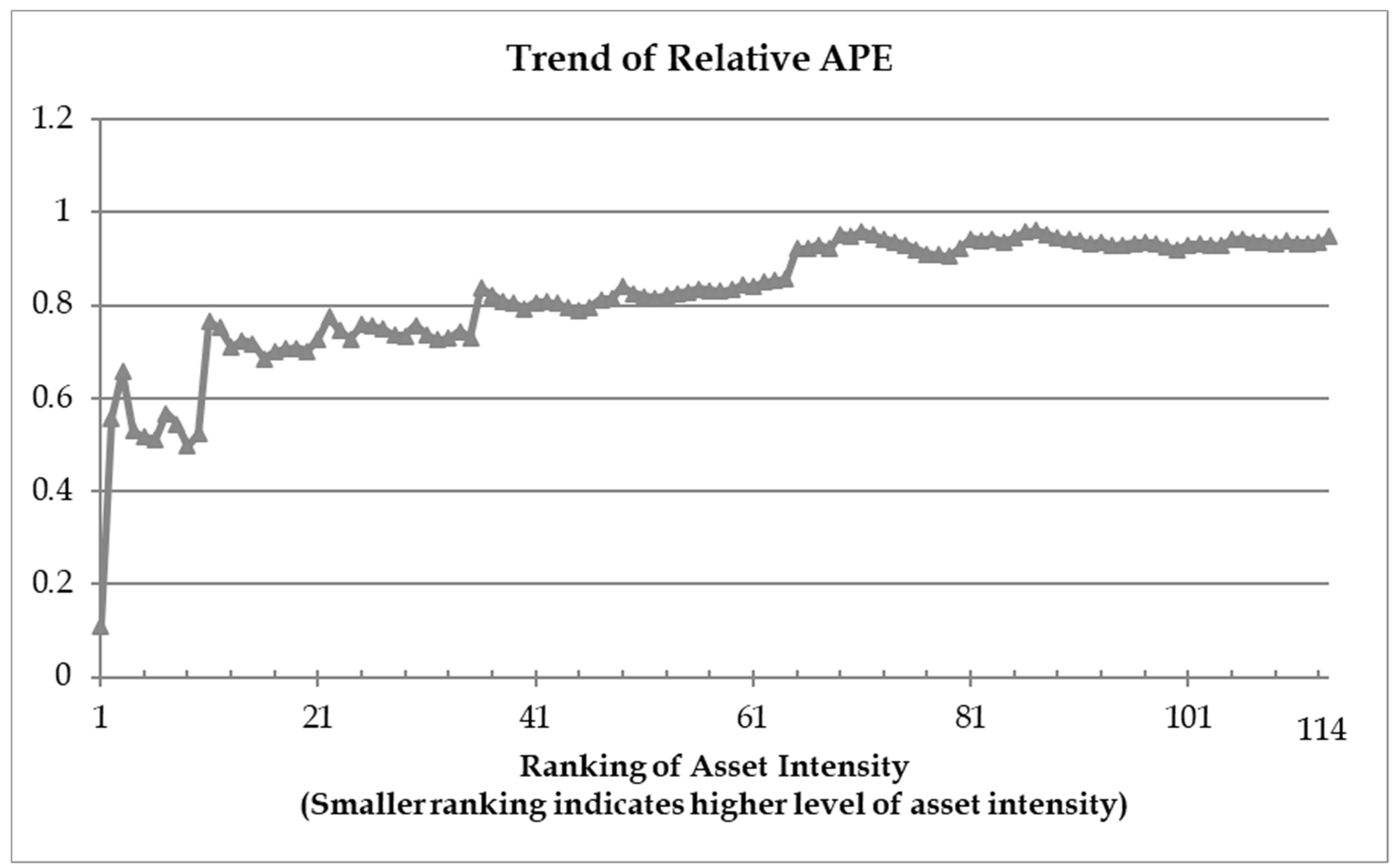
Figure 1 plots the trend of relative APE against asset intensity. Asset intensity is measured as the ratio of total assets to sales. Smaller ranking on the horizontal axis indicates higher level of asset intensity. The relative APE in Figure 1 shows a clear upward trend. This indicates that the predictive gain from using the quarterly data is relatively large for asset intensive industries (smaller ranking on the horizontal axis). However, this gain diminishes for asset light industries (higher ranking on the horizontal axis). The results are consistent with our expectations.

Figure 1 plots the trend of the relative APE (mid-year quarterly update relative to annual data) across the industry portfolios (formed based on four-digit SIC code) in our sample. The industry sectors are ranked by asset intensity (measured by the ratio of total assets to sales) on the horizontal axis. Smaller ranking indicates higher level of asset intensity. The values on the vertical axis indicate the cumulative relative APE values based on the forecast performance using the mid-year quarterly update compared with previous year’s annual data. Relative APE values that are less than 1 indicate that the quarterly updates lead to improvements in the predictive performance. The trend of the relative APE indicates how asset intensity is associated with the predictive gain from using the quarterly data. The increasing trend indicates that the predictive gain from using the quarterly data is relatively large for asset intensive industries (smaller ranking on the horizontal axis), and the gain diminishes as the asset intensity increases.

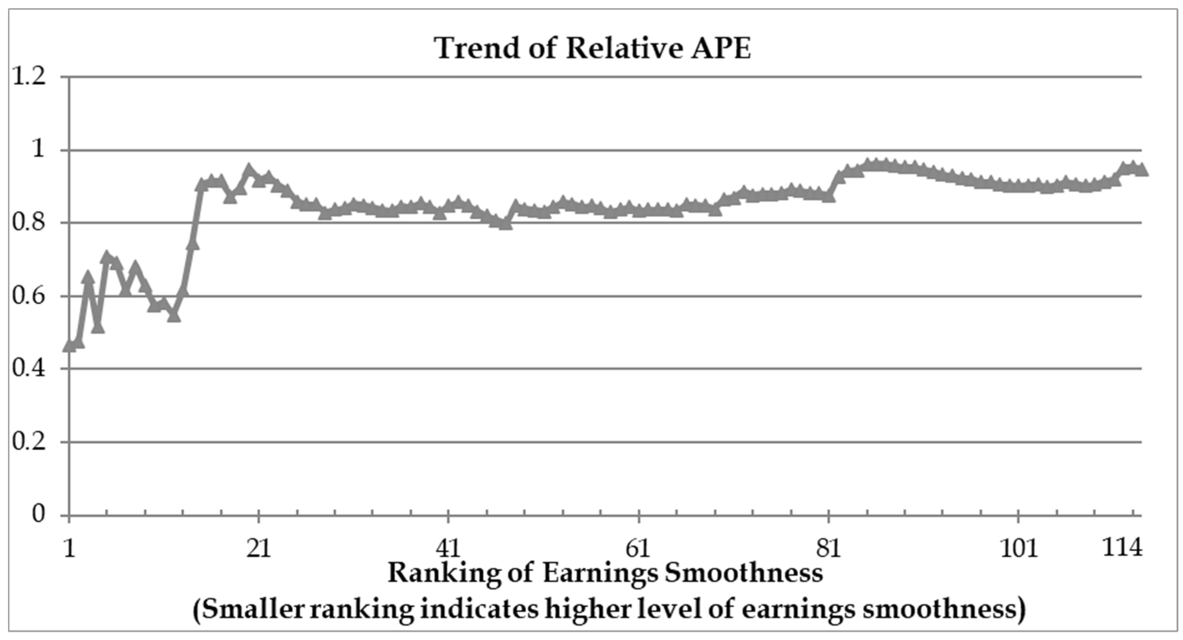
Figure 2 plots the trend of relative APE against earnings smoothness. Earnings smoothness is measured as the reciprocal of earnings volatility (the standard deviation of accounting earnings E) scaled by cash flow volatility (the standard deviation of operating cash flows CF) on the horizontal axis. Smaller ranking on the horizontal axis indicates higher level of earnings smoothness.5

Figure 2 plots the trend of the relative APE (mid-year quarterly update relative to annual data) across the industry portfolios (formed based on four-digit SIC code) in our sample. The industry sectors are ranked by earnings smoothness. Earnings smoothness is measured as the reciprocal of earnings volatility (the standard deviation of accounting earnings) scaled by cash flow volatility (the standard deviation of operating cash flows) on the horizontal axis. Smaller ranking indicates higher level of earnings smoothness. The values on the vertical axis indicate the cumulative relative APE values based on the forecast performance using the mid-year quarterly update compared with previous year’s annual data. Relative APE values that are less than 1 indicate that the quarterly update leads to improvements in the predictive performance. The trend of the relative APE indicates how earning smoothness is associated with the predictive gain from using the quarterly data. The increasing trend indicates that the predictive gain from using the quarterly data is relatively large for asset with higher level of earnings smoothness (smaller ranking on the horizontal axis), and the gain diminishes as the earnings smoothness decreases.

Consistent with our expectation, Figure 2 show that the predictive gain from using quarterly data is more pronounced for industries with high levels of earnings smoothness (on the far-left end of the horizontal axis). By contrast, industries characterized by highly volatile earnings exhibits little improvement in forecast performance from using quarterly data, with the relatively APE approaching 1 for the industries on the far-right end of the horizontal axis.

Overall, the results in this section show that the predictive gain from using quarterly information is not universal and there is considerable variation across industries. Quarterly reporting significantly improves the ability to predict future operating cash flows for some industry sectors but makes little difference in forecasting performance for other sectors. These findings have practical implications. Particularly, investors in portfolios or funds that are heavily weighted in industries known for generating stable cash flows can benefit more from paying closer attention to firms’ interim financial results.

5. Conclusions

A fundamental role of financial reporting is to provide information useful in forecasting future cash flows. Previous accounting research on cash flow forecasting mostly focuses on annual financial statements despite the widely assumed importance of quarterly reports to the capital market. In this paper, we extend the literature by examining the usefulness of quarterly financial statements in predicting future operating cash flows.

We find that using the time series of quarterly data available at the end of the previous year to forecast the current year’s annual operating cash flows results in lower forecast error than using the time series of annual data. As this reduction in forecast error cannot be attributed to “new” information from quarterly updates during the current year, our results suggest that shorter reporting intervals can help improve the forecasting performance in predicting future operating cash flows by better revealing the trend of the time-series relationship between financial statement information and future cash flows. This finding adds to the evidence from previous research that the usefulness of accounting information is not confined to the “news role” (Drake et al. 2016) and provides new insights on why the frequency of financial reporting matters. In addition, we document evidence that quantifies the effects of new quarterly updates on forecasting performance. Our findings contribute to the literature that examines the different aspects of the impact of financial reporting frequency on the capital market (Alves and Dos Santos 2008; Arif and De George 2020; Ernstberger et al. 2017; Fu et al. 2012; Kraft et al. 2018; Pozen et al. 2017). Moreover, we find that the improvement in forecast performance from using quarterly data is not universal and there is considerable variation across industries. We show that the predictive gain from using quarterly data is larger for asset-heavy industries and industries with higher levels of earnings smoothness.

The results of this study have important policy implications. During recent years, businesses and regulators around the world are increasingly debating the benefits and costs of more frequent interim reporting. The European Union introduced mandatory quarterly reporting for listed companies in 2007 but decided to scrap the requirement and returned to semi-annual reporting in 2013. In the United States, the Security Exchange Commission is considering the pros and cons of moving to less frequent semi-annual reporting from the current regime of quarterly reporting, which has been the standard in the U.S. since the 1930’s. Empirical evidence on the out-of-sample predictive ability of quarterly financial statements as documented in this study helps ensure an informed debate over this issue.

Our findings have direct policy implications for the ongoing debate concerning the “optimal” reporting frequency to be mandated in the capital market. Previous research demonstrates that financial reporting environments represent an important institutional factor that plays a significant role in shaping the governance quality of a country both on the micro and macro levels. For example, Siriopoulos et al. (2021) document that adoption of International Financial Reporting Standards (IFRS) is a strong determinant that promotes foreign direct investments in countries of the Gulf Cooperation Council. A better understanding of why the frequency of financial reporting matters can help inform the ongoing debates and the policy decisions on the frequency of financial reporting requirements. Future research may explore how financial reporting frequency interacts with firm characteristics and institutional factors to affect the information environment of the capital market.

References

- Alves, Carlos F., and Fernando T. Dos Santos. 2008. Do first and third quarter unaudited financial reports matter? The Portuguese case. European Accounting Review 17: 361–92. [Google Scholar] [CrossRef]
- Arif, Salman, and Emmanuel T. De George. 2020. The dark side of low financial reporting frequency: Investors’ reliance on alternative sources of earnings news and excessive information spillovers. The Accounting Review 95: 23–49. [Google Scholar] [CrossRef]
- Barth, Mary E., Donald. R. Cram, and Karen K. Nelson. 2001. Accruals and the prediction of future cash flows. The Accounting Review 76: 27–58. [Google Scholar] [CrossRef]
- Brown, Philip, and Victor Niederhoffer. 1968. The predictive content of quarterly earnings. Journal of Business 41: 488–97. [Google Scholar] [CrossRef]
- Brown, Lawrence D., and Michael Rozeff. 1979. The predictive value of interim reports for improving forecasts of future quarterly earnings. The Accounting Review 54: 585–91. [Google Scholar]
- Cleveland, Robert B., William S. Cleveland, Jean E. McRae, and Irma Terpenning. 1990. STL: A seasonal-trend decomposition procedure based on loess. Journal of Official Statistics 6: 3–73. [Google Scholar]
- Coates, Robert. 1972. The predictive content of interim reports—A time series analysis. Journal of Accounting Research 10: 132–44. [Google Scholar] [CrossRef]
- Dechow, Patricia M. 1994. Accounting earnings and cash flows as measures of firm performance: The role of accounting accruals. Journal of Accounting and Economics 18: 3–42. [Google Scholar] [CrossRef]
- Dechow, Patricia M., Weili Ge, and Catherine M. Schrand. 2010. Understanding earnings quality: A review of the proxies, their determinants and their consequences. Journal of Accounting and Economics 50: 344–401. [Google Scholar] [CrossRef] [Green Version]
- Dechow, Patricia M., S. P. Kothari, and Ross L. Watts. 1998. The relation between earnings and cash flows. Journal of Accounting and Economics 25: 133–68. [Google Scholar] [CrossRef] [Green Version]
- Drake, Michael S., Darren T. Roulstone, and Jacob R. Thornock. 2016. The usefulness of historical accounting reports. Journal of Accounting and Economics 61: 448–64. [Google Scholar] [CrossRef]
- Ernstberger, Jürgen, Benedikt Link, Michael Stich, and Oliver Vogler. 2017. The real effects of mandatory quarterly reporting. The Accounting Review 92: 33–60. [Google Scholar] [CrossRef]
- Farshadfar, Shadi, and Reza Monem. 2013. Further evidence on the usefulness of direct method cash flow components for forecasting future cash flows. The International Journal of Accounting 48: 111–33. [Google Scholar] [CrossRef] [Green Version]
- Financial Accounting Standards Board. 1978. Statement of Financial Accounting Concepts No. 1: Objectives of Financial Reporting by Business Enterprises. Norwalk: Financial Accounting Standards Board. [Google Scholar]
- Foster, George. 1977. Quarterly accounting data: Time-series properties and predictive-ability results. The Accounting Review 52: 1–21. [Google Scholar]
- Fu, Renhui, Arthur G. Kraft, and Huai Zhang. 2012. Financial reporting frequency, information asymmetry, and the cost of equity capital. Journal of Accounting and Economics 54: 132–49. [Google Scholar] [CrossRef]
- Hui, Kai Wai, Karen K. Nelson, and P. Eric Yeung. 2016. On the persistence and pricing of industry-wide and firm-specific earnings, cash flows, and accruals. Journal of Accounting and Economics 61: 185–202. [Google Scholar] [CrossRef]
- Hyndman, Rob J., and George Athanasopolous. 2018. Forecasting: Principles and Practice, 2nd ed. Heathmont: OTexts. [Google Scholar]
- Kim, Myungsun, and William Kross. 2005. The ability of Earnings to predict future operating cash flows has been increasing—Not decreasing. Journal of Accounting Research 43: 753–80. [Google Scholar] [CrossRef]
- Kraft, Arthur G., Rahul Vashishtha, and Mohan Venkatachalam. 2018. Frequent financial reporting and managerial myopia. The Accounting Review 93: 249–75. [Google Scholar] [CrossRef]
- Krishnan, Gopal V., and James A. Largay III. 2000. The predictive ability of direct cash flow information. Journal of Business Finance and Accounting 27: 215–45. [Google Scholar] [CrossRef]
- Rundo, Francesco, Francesca Trenta, Agatino Luigi di Stallo, and Sebastiano Battiato. 2019. Machine learning for quantitative finance applications: A survey. Applied Sciences 9: 5574. [Google Scholar] [CrossRef] [Green Version]
- Pozen, Robert, Suresh Nallareddy, and Shivaram Rajgopal. 2017. The impact of reporting frequency on UK public companies. The CFA Research Foundation Briefs 2017-B1: 1–20. [Google Scholar]
- Siriopoulos, Costas, Athanasios Tsagkanos, Argyro Svingou, and Evangelos Daskalopoulos. 2021. Foreign Direct Investment in GCC countries: The essential influence of corporate governance and the adoption of IFRS. Journal of Risk andFinancialManagement 14: 264. [Google Scholar] [CrossRef]
- Tsagkanos, Athanasios, Konstantinos Gkillas, Christoforos Konstantatos, and Christos Floros. 2021. Does volume drive systemic banks’ stock return volatility? Lessons from the Greek banking system. International Journal of Financial Studies 9: 24. [Google Scholar] [CrossRef]
Figure 1.
Asset intensity and the predictive gain from using quarterly data.
Figure 2.
Earnings smoothness and the predictive gain from using quarterly data.