Article

Land Cover Impacts on Surface Temperatures: Evaluation and Application of a Novel Spatiotemporal Weighted Regression Approach

1
Department of Computer Science, University of Idaho, Moscow, ID 83844, USA
2
College of Computer and Information Sciences, Fujian Agriculture and Forestry University, Fuzhou 350002, China
3
Department of Earth and Spatial Sciences, University of Idaho, Moscow, ID 83844, USA
4
Earth and Planets Laboratory, Carnegie Institution for Science, Washington, DC 20015, USA
*
Author to whom correspondence should be addressed.
ISPRS Int. J. Geo-Inf. 2023, 12(4), 151; https://doi.org/10.3390/ijgi12040151
Submission received: 27 January 2023 / Revised: 27 March 2023 / Accepted: 31 March 2023 / Published: 3 April 2023

Abstract

:
The urban heat island (UHI) effect is an important topic for many cities across the globe. Previous studies, however, have mostly focused on UHI changes along either the spatial or temporal dimension. A simultaneous evaluation of the spatial and temporal variations is essential for understanding the long-term impacts of land cover on the UHI. This study presents the first evaluation and application of a newly developed spatiotemporal weighted regression framework (STWR), the performance of which was tested against conventional models including the ordinary least squares (OLS) and the geographically weighted regression (GWR) models. We conducted a series of simulation tests followed by an empirical study over central Phoenix, AZ. The results show that the STWR model achieves better parameter estimation and response prediction results with significantly smaller errors than the OLS and GWR models. This finding holds true when the regression coefficients are constant, spatially heterogeneous, and spatiotemporally heterogeneous. The empirical study reveals that the STWR model provides better model fit than the OLS and GWR models. The LST has a negative relationship with GNDVI and LNDVI and a positive relationship with GNDBI for the three years studied. Over the last 20 years, the cooling effect from green vegetation has weakened and the warming effect from built-up features has intensified. We suggest the wide adoption of the STWR model for spatiotemporal studies, as it uses past observations to reduce uncertainty and improve estimation and prediction results.

1. Introduction

The urban heat island (UHI) effect is among the greatest short-term threats to the biophysical environment and human health. Significant warming in densely built urban areas compared to rural areas has caused a range of environmental, economic, and energy impacts such as elevated emissions of greenhouse gases, impaired air quality, and increased energy consumption [1]. Further, the UHI effect can increase both the magnitude and duration of a heat wave, causing adverse impacts on human health, particularly in vulnerable populations [2].
The UHI effect is a global issue, and UHI studies have been conducted in many cities around the world. Numerous studies have focused on the relationships between UHIs and the land surface temperature (LST) with different land cover types and patterns [3,4,5]. Among major land cover types, green vegetation, such as trees and grass, and impervious surfaces, such as roads, pavements, and parking lots, are key contributors to LST variations [6,7,8]. Apart from land composition, spatial characteristics such as shape, orientation, and spatial arrangement can have a sizable impact on the LST as well [9,10]. Understanding the spatiotemporal impacts of land-use/land cover change on the UHI effect is important for making informed decisions on urban planning and natural resource management. Further, as increasing numbers of cities are becoming aware of the detrimental effects of urban warming, mitigation strategies are being implemented at a global scale. A better understanding of the changing patterns of the UHI effect is vital for evaluating the effectiveness of these mitigation measures.
A suite of statistical tools has been used in UHI studies. The ordinary least squares (OLS) regression model is widely used to study linear relationships between the UHI effect and its drivers [11,12]. More advanced statistical models such as the generalized addictive model, random forest regression, and artificial neural networks have been increasingly employed to address more complex relationships such as non-linear relationships [13,14,15]. Global models assume a static statistical relationship based on the entire geographical region. This can be problematic, especially when the study area is quite large as there might be multiple spatial processes occurring at different spatial scales. The geographically weighted regression (GWR) model was developed to address spatial non-stationarity [16]. For each observation, the GWR borrows data from its neighbors as defined by the spatial weights matrix and calibrates a separate model [17].
While local spatial variations are addressed using models such as the GWR model, it remains a challenge to effectively incorporate variations in the temporal dimension. There have been efforts dedicated to developing spatiotemporal models to account for both spatial and temporal effects. Huang et al. [18] proposed a geographically and temporally weighted regression (GTWR) model that incorporated both spatial and temporal effects into the weighting matrices. However, Fotheringham et al. [19] pointed out that the simple integration of spatial and temporal distances in the GTWR could be misleading as they are measured at varying scales. Que et al. [20] proposed a novel spatiotemporal model named the spatiotemporally weighted regression (STWR) model. The STWR model was built based on the assumption that the rate of value change in time has an impact on the value of its nearby locations. Building upon the GWR, the STWR model addresses both spatial and temporal heterogeneity by borrowing data points not only from nearby locations in space but also from nearby attribute variations over time [20]. In contrast to the GTWR model, which considers distance over time, the STWR model focuses on the rate of nearby data variation over time and reflects the temporal effect of observations near the regression point.
Our study presents the first evaluation and application of the STWR method in comparison to conventional models in the context of a surface UHI study. Satellite image-derived biophysical land cover indicators and LST products were used. A series of systematically designed simulation experiments were set up to assess the performance of the STWR in comparison with the OLS and GWR. We further conducted an empirical study over Phoenix, AZ, to evaluate the evolving relationships between the LST and land cover changes. Our study aims to achieve the following objectives: (1) to compare the performance of the STWR method with that of the OLS and GWR models in terms of parameter estimation and response prediction and (2) to understand the way in which the LST–land cover relationship changed over 20 years in a rapidly urbanizing desert region.
The rest of the article is organized as follows: Section 2 describes the study area and introduces the variables, models, and parameters used in the simulation experiments. It also describes the metrics used to evaluate the performance of the models. Section 3 reports the results of the simulation for three case scenarios. Section 4 presents an empirical study where the STWR models were applied to understand the spatiotemporal relationships between LST and land cover patterns over central Phoenix. Section 5 discusses the performance and advantages of the STWR and highlights the implications of the findings on urban cooling. Section 6 summarizes the study and proposes future directions.

2. Materials and Methods

2.1. Study Area

Our study focuses on central Phoenix, which is located in the northern part of the Sonoran Desert (Figure 1). Phoenix is in one of the sunniest regions in the world, with an average of 300 days of sunshine per year [21]. It has a hot desert climate with extremely hot, dry summers and mild, short winters. Unlike other desert cities with a large day–night temperature difference, Phoenix has a constantly high temperature due to its phenomenal UHI effect. The UHI is steadily intensifying as the city continues to expand, resulting in significantly elevated temperatures. The average summer temperature in Phoenix was 26.8 °C in 2000 but had increased to 36.1 °C by 2020 [22]. Heat waves have become more frequent and intense, contributing to the further intensification of the UHI effect. Understanding the spatiotemporal patterns of the UHI in connection with land cover change is vital for developing effective mitigation measures for the well-being of the residents, especially those susceptible to extreme heat.

2.2. Simulation Experiments

We conducted a series of simulation experiments to evaluate the performance of the OLS, GWR, and STWR models in terms of parameter estimation and response prediction. In the simulation, true coefficient surfaces were artificially generated with three case scenario settings: (1) the coefficient surfaces are constant both spatially and temporally, (2) the coefficient surfaces are spatially heterogeneous but temporally constant, and (3) the coefficient surfaces have both spatial and temporal variations. Figure 2 presents the workflow of the simulation. The rest of this section describes the simulation process in detail.

2.2.1. Variable Setting

There were three independent variables in the model, all of which were derived from Landsat images over Phoenix. We used all available images from June to August with a cloud cover under 10% because daytime temperatures are highest and the relationship between LST and land cover is strongest in the summer [23]. For each year, the Landsat images were integrated into a summer composite. The performance of the OLS, GWR, and STWR models was tested for the year of 2020. For the OLS and GWR models, only the summer composite for 2020 was used, as no temporal effects were considered. For the STWR model, in addition to the 2020 data, we used additional summer composite images in 2000, 2005, 2010, and 2015 to account for their temporal impacts on the 2020 data. We focused on two major land cover types in the study area: vegetation and built-up areas. We used the normalized difference vegetation index ( N D V I ) to represent the green biomass (Equation (1)) and the normalized difference built-up index ( N D B I ) to represent the built-up features in the region (Equation (2)).
N D V I = N I R R E D N I R + R E D ,
N D B I = S W I R R E D S W I R + R E D ,
where NIR, RED, and SWIR stand for the near-infrared band, red band, and short-wave infrared band, respectively.
We used spatial autocorrelation indices to characterize the landscape pattern. The Getis-Ord G measures the local abundance of a particular land cover. Mathematically, the Getis-Ord G for location i, G i d , is provided by
G i d = j w i j d x j j x j ,
where x j denotes the attribute value at a particular location j. We used a row-standardized binary spatial weights matrix with a radius distance of 150 m following previous studies [24,25]. We calculated the z-score, which is the standardized Getis-Ord G. A high z-score means a spatial clustering of high values (hot spot), and a low z-score means a spatial clustering of low values (cold spot). Both high and low z-scores are relative to the average of the image. We calculated the Getis-Ord G for the NDVI and NDBI to measure the local abundance of vegetation and built-up features, respectively.
The local Moran’s I was used to quantify the degree of spatial clustering, and it is provided by
I i d = n x i x ¯ i x i x ¯ 2 j w i j d x j x ¯ ,
where x i denotes the attribute value at a particular location i. We used the same spatial weights matrix and radius distance in the calculation of the local Moran’s I. Unlike the Getis-Ord G, a high positive z-score means a spatially clustered pattern (either high values or low values), and a low negative z-score means a spatially dispersed pattern. Note that the local Moran’s I focuses on the spatial arrangement rather than the absolute data values, and it was calculated for NDVI only as the local Moran’s I of NDBI reveals a similar spatial pattern.
Rather than using observed data, the values on the dependent variable in the simulation were generated following a data-generating process (Section 2.2.3). There were three scenario settings, and each one was tested with three regression models (i.e., the OLS, GWR, and STWR models).

2.2.2. Model Formulation

The classic OLS model can be formulated as
y i = β 0 + k = 1 β k   x i k + ε i ,
where y i denotes the dependent variable at location i , β k is the regression coefficient associated with the k th independent variable x i k , and ε i is a random error term.
The GWR model extends the OLS by allowing the local regression coefficients to vary spatially, and it is formulated as
  y i = β 0 u i , v i + k = 1 β k u i , v i x i k + ε i ,
where x i k is the k th independent variable at location u i , v i and β k u i , v i is the regression coefficient associated with the k th independent variable at location u i , v i .
The STWR [20] further extends the GWR by borrowing past observations to improve model performance at a certain time t . A typical STWR model can be expressed as
y i t = β 0 t u i , v i + k = 1 β k t u i , v i x i k t + ε i t ,
where x i k t is the k th independent variable at location u i , v i at time t , β k t u i , v i denotes the k th regression coefficient at location u i , v i at time t , and ε i t is a random error term with a Gaussian distribution.
The model calibration is provided by
β ^ k t u i , v i = ( X T W t u i , v i X ) 1 X T W t u i , v i y i t ,
where X is the matrix form of the independent variables. W t u i , v i denotes a diagonal weighting matrix at location u i , v i . The STWR uses a novel rate-of-change decay weighting strategy to weight local temporal effects. The new weighted average form of the spatiotemporal kernel takes the form
w i j S T t = 1 α K s d s i j , b S T + α K T d t i j , b T ,   0 α 1 ,
where w i j S T t is the element of the matrix W t u i , v i in Equation (6), which denotes the spatiotemporal weight on the observed location j at time t ; K s and K T are the spatial and temporal kernels, respectively, which range from 0 to 1; α is an adjustable parameter that can be optimized in the model calibration process; b S T denotes the spatial bandwidth at a particular time T ; b T is the temporal bandwidth; and d s i j and d t i j represent the spatial and temporal distance between location i and j , respectively. The temporal kernel K T that can generate the temporal weights w i j Δ t t of the STWR framework is specified as
w i j Δ t t = 2 1 + e x p ( y i t y j t q / y j t q Δ t / b T ) 1 , i f   0 < Δ t < b T 0 , otherwise ,
where Δ t is the time interval and | ( y i t y j t q ) / y j t q | is the absolute different rate between the observed value for regression point i at t and the observed value for point j at t q . The weight is set to zero if the time interval falls out of 0 ,   b T . The STWR allows the spatial bandwidth to vary over time. The spatial kernel K s takes the form of a bi-square kernel, a Gaussian kernel, or another spatial kernel. w i j S T t is obtained by substituting K s and K T into Equation (7).

2.2.3. Simulation Parameter Setting

The simulation experiments were set up based on the assumption that the true coefficient surfaces were known. We tested a total of three case scenarios with different settings of the coefficient surfaces.
For case scenario 1, the data-generating equation is provided by
y = 1 + 2 G N D B I 2 G N D V I 1 L N D V I + e r r ,
where G N D B I , G N D V I , and L N D V I represent the Getis-Ord G of NDBI, the Getis-Ord G of NDVI, and the local Moran’s I of NDVI, respectively. e r r is an error term randomly drawn from the Gaussian distribution N (0, 4).
In the second case scenario, the beta surfaces were set up as
β 0 u i , v i = 2 ,
β 1 u i , v i = 2 + u i + v i / 353   ( 0 < u i , v i < 353 ) ,
β 2 u i , v i = 1 + 3 2 u i 90 2 3 2 v i 90 2 2   0 < u i , v i < 353 ,
β 3 u i , v i = 0.2 s i n π 100 u i + v i 2.5 2   ( 0 < u i , v i < 353 ) .
Note that each beta surface was a 353 × 353 matrix. The data-generating equation is provided by
y i = β 0 u i , v i + β 1 u i , v i G N D B I + β 2 u i , v i G N D V I + β 3 u i , v i L N D V I ± e r r i       0 < u i , v i < 353 ,
where e r r i is a random error term drawn from the Gaussian distribution N (0, 2).
For case scenario 3, the beta coefficients were generated using the following equations:
β 0 t u i , v i = β 0 t 1 u i , v i + 0.1 s i n v i 40 Δ t   0 < u i , v i < 353 ,
β 1 t u i , v i = β 1 t 1 u i , v i + 0.1 s i n π 100 u i Δ t   0 < u i , v i < 353 ,
β 2 t u i , v i = β 2 t 1 u i , v i + 0.1 s i n π 60 u i + v i Δ t   0 < u i , v i < 353 ,
β 3 t u i , v i = β 3 t 1 u i , v i + 0.1 s i n π 160 u i + v i Δ t   0 < u i , v i < 353 .
The coefficients at the initial time stage were set up as
β 0 0 u i , v i = 2 + 0.5 s i n v i 40   0 < u i , v i < 353 .
β 1 0 u i , v i = 2 + u i + v i 353 + 0.5 s i n π 100 u i   0 < u i , v i < 353 ,
β 2 0 u i , v i = 1 + 3 2 u i 90 2 3 2 v i 90 2 2 + 0.5 s i n π 60 u i + v i 0 < u i , v i < 353 ,
β 3 0 u i , v i = 0.2 s i n π 100 u i + v i 2.5 2 + 0.5 s i n π 160 u i + v i   ( 0 < u i , v i < 353 ) .
The data-generating equation is
y i t = β 0 t u i , v i + β 1 t u i , v i G N D B I + β 2 t u i , v i G N D V I + β 3 t u i , v i L N D V I ± e r r i       0 < u i , v i < 353 ,
where e r r i is a random error term drawn from the Gaussian distribution N (0, 2).
For each year, a total of 1000 samples were randomly selected, and the regression models were fit for the year 2020. For the OLS and GWR models, only the samples in 2020 were utilized because no temporal effects were considered. For the STWR model, all previous years’ samples were included in addition to the samples in 2020 to account for their temporal effects. In addition to the coefficient surfaces, we also generated response surfaces for comparison. For all three models, the process was replicated 100 times to obtain an averaged estimation of the coefficients and responses. All the simulated experiments were implemented using the Fast-STWR package in Python (https://github.com/quexiang/Fast-STWR (accessed on 20 July 2022)).

2.2.4. Assessment Metrics

The performance of the three models was assessed as follows. First, for each fitting method, a total of 100 beta estimation surfaces were generated for each beta coefficient. The 100 estimation surfaces were averaged pixel by pixel to provide four mean estimation surfaces (one for each beta coefficient). Second, we subtracted the original true beta surfaces from the mean estimation surfaces to obtain estimation error surfaces. Third, we used the absolute value of the estimation error surfaces to generate four absolute error surfaces. Lastly, we calculated the mean of the absolute error over the surface (spatial average) and obtained a mean absolute error (MAE) score for each coefficient.
The response prediction was assessed in a similar manner. For each fitting method, the 100 response surfaces were averaged pixel by pixel to provide a mean response surface. We then subtracted the data-generated response surface from the mean response surface to obtain estimation error surfaces. We calculated the absolute value of each estimation error surface, yielding three absolute error response surfaces. These surfaces were spatially averaged to obtain the MAE for each fitting method. In addition to the MAE, we also calculated the Akaike information criterion (AIC) [26] at each replication to provide an averaged AIC score for each fitting method.

3. Simulation Results

3.1. Simulation Case Scenario 1—Constant Coefficients

In the first simulation, the beta coefficients were both spatially and temporally constant (Figure 3). Figure 3 shows the estimation error surfaces for the OLS, GWR, and STWR model, respectively. Because the OLS model is a global model, the estimation error surfaces are spatially constant. There were spatial variations in the GWR and STWR models because these two models allow the coefficients to vary spatially. When comparing the three models, the STWR model achieved the smallest estimation error for all four coefficients despite the spatial variations. The OLS model ranked second, and the GWR model had the largest estimation error.
Table 1 shows the MAE scores for the beta coefficient surfaces obtained from the OLS, GWR, and STWR models. These results were generated from Case Scenario 1, which assumes that the beta coefficients are spatially and temporally constant. Consistent with the estimation error surfaces in Figure 4, the STWR model had the lowest MAE score for all coefficients, followed by the OLS and GWR models, respectively. As all coefficients were set to be spatiotemporally constant, a global model would be suitable for identifying the relationships. This largely explained the good performance of the OLS model in comparison with the GWR model. However, even with spatially constant coefficients, the STWR model still performed the best and achieved the smallest overall estimation error.
In addition to parameter estimation, we also obtained the response surfaces for the year 2020 using the OLS, GWR, and STWR models. We then calculated the response estimation error by subtracting the data-generated response surface from each fitted response surface. The data-generated response surface is the response surface obtained from the data-generating process. Figure 5 shows the response estimation error surfaces. We could hardly pinpoint any differences in the three models by studying the error surfaces alone. When examining the MAE scores (Table 2), the OLS model had a slightly lower MAE than the GWR (0.035 difference) and STWR (0.033 difference) models. The AIC score did not reveal any significant differences either, although the GWR model had a slightly larger AIC than the other two.

3.2. Simulation Case Scenario 2—Spatially Varying Coefficients

In the second simulation, the four coefficient surfaces were set up to show varying degrees of spatial heterogeneity, but there was no temporal variation (Figure 6). Figure 7 shows the estimation error surfaces for the three models based on spatially varying coefficients. We determined that the spatial patterns in the error surfaces obtained from the OLS model resemble those of the true beta coefficients. This is not surprising because, as a global model, the OLS model generates spatially constant coefficients. On average, the OLS model had the largest estimation error among the three models. The two local models performed better in terms of parameter estimation, with the STWR having a smaller estimation error than the GWR according to a visual inspection. The good performance of the STWR model was corroborated by the MAE scores shown in Table 3. From Table 3, the STWR had the lowest MAE scores for all coefficients. The GWR model had higher MAE scores than the STWR model but lower MAE scores than the OLS model, with the sole exception of beta 3.
Figure 8 shows the estimation error surfaces for the response. In contrast to Case Scenario 1 where the coefficients were constant, with spatially varying coefficients, the STWR model seemed to have the smallest overall response estimation error. The GWR model showed a small amount of overestimation, whereas the OLS model showed strong overestimation across the study area. The MAE score told the same story, with the STWR model showing the lowest MAE score followed by the GWR and OLS models, respectively (Table 4). The STWR also achieved the best fit with the data on average based on the AIC score.

3.3. Simulation Case Scenario 3—Spatiotemporally Varying Coefficients

In the third simulation, the coefficient surfaces involved not only spatial variations but also temporal variations (Figure 9). Figure 10 shows the estimation error surfaces for the three models. As with Case Scenario 2, the coefficient patterns of the OLS model were somewhat similar to the original ones given that it assumes a spatiotemporally constant coefficient surface. While the local models showed quite a bit of spatial variations in the coefficient surfaces, the OLS model yielded relatively stable patterns with no abrupt changes. Comparing the GWR and STWR surfaces, all GWR surfaces had several over/under-estimated areas with significant spatial clustering. The GWR model also had more pixels with large estimation errors than the STWR model. The estimation errors for the STWR model seemed to be random and small across the study area. Table 5 confirms that the STWR model had the lowest MAE scores for all the coefficients. The MAE scores of the GWR model were a little higher than those of the STWR model but lower than those of the OLS model, with the sole exception of beta 3.
Figure 11 shows the estimation error surfaces for the response. The OLS model showed a significant number of overestimated pixels, and the GWR model had a relatively balanced number of overestimated and underestimated pixels. From the figure, we can see that the STWR model achieved the smallest estimation error on average. A similar pattern can be observed in Table 6, with the STWR model having the lowest MAE score. When coefficients have spatiotemporal variations, the STWR also provides the best goodness of fit for the data.

4. Empirical Study

In addition to the simulation experiments, we performed an empirical study to understand the impacts of land cover patterns on the LST in 2000, 2010, and 2020 over central Phoenix, AZ. We further compared the model goodness of fit achieved by the three models.
In a similar manner to the simulation experiments, the independent variables were the Getis of NDVI, the Getis of NDBI, and the local Moran’s I of NDVI (see Section 2.2.1 for calculation). Instead of using synthetic data as in the simulation, real-world LST data were adopted for the dependent variable. We used the Landsat Level-2 Provisional Surface Temperature product from the USGS [27], which has been widely utilized in numerous scientific studies and applications [28,29,30]. The LST product was generated using the Landsat Ecosystem Disturbance Adaptive Processing System (LEDAPS) algorithm [31]. The LEDAPS algorithm is based on radiative transfer theory and uses a combination of empirical and physically based models to estimate the surface temperature [32]. We obtained the LST data for 2000, 2010, and 2020 for the same dates as the Landsat images and created a summer composite for each year. A total of 3000 random samples were selected for each year, and they were kept the same for the three regression models. For the OLS and GWR models, only data from one year were used—data collected in 2020 were used in the 2020 model. For the STWR model, all historically observed data points were initially included in the model. The final observations depend on the optimal temporal bandwidth determined in the model fitting process. For instance, when fitting the STWR model for 2020, the historical observations from 2000 and 2010 were included in conjunction with the 2020 observations. If the optimal temporal bandwidth were two, the actual observations used by the STWR model would include data points from both 2020 and 2010.
Table 7 shows the R2 for the three regression models for 2000, 2010, and 2020. The R2 scores were above 0.5 for the OLS models, and above 0.9 for the STWR models across all years. For all three years, the STWR model outperformed the OLS and GWR models, as is indicated by it having the highest R2 among the three models. The highest R2 score was 0.948 in 2020.
Table 8 shows the mean coefficient estimates for the STWR model. Only significant estimates were included in the calculation. For all three years, the GNDVI and LNDVI had negative relationships with the LST, and the GNDBI had a positive relationship with the LST. From 2000 to 2010, the mean coefficient of the GNDVI decreased, indicating a weakening cooling effect from the green vegetation. The warming effect from built-up features, on the other hand, intensified over the 20 years as is reflected by the increasing positive coefficient of the GNDBI. The negative coefficient of the local Moran’s I suggested that a clustered pattern of green vegetation had a positive impact on urban cooling. The impact, however, declined from 2000 to 2020.
To understand the relationship between land cover patterns and LST for different land-use/land cover zones, we further calculated the mean coefficient estimates by major land cover type in the region. The land cover data were sourced from the National Land Cover Database (NLCD) from 2001, 2011, and 2019 (Figure 12). According to Figure 12, there are four major types of land cover in the study area, including developed high intensity, developed medium intensity, developed low intensity, and developed open space. The developed high intensity category includes high-intensity commercial areas, industrial areas in downtown Phoenix, and transportation areas near the Sky Harbor Airport. The developed medium intensity category primarily includes the medium-intensity single-family residential areas. Low-intensity single-family residential areas are categorized as developed low-intensity. Recreational areas such as parks, golf courses, and other vegetated areas are classified as developed low-intensity or developed open-space depending on the fraction of green vegetation in the area.
Table 9 shows the mean significant estimates for GNDVI, GNDBI, and LNDVI by land cover type for the three years. First, there was a negative relationship between the GNDVI and LST, and the relationship weakened over time across all land cover types. The strongest cooling effect from green vegetation was observed in developed high intensity in 2000 and changed to developed open space in 2010 and 2020. The GNDBI had a consistently positive relationship with the LST, and the warming effect intensified from 2000 to 2020 for nearly all land cover types. The strongest warming effect occurred in low- and medium-intensity developed areas in 2020, and in developed open space in 2000 and 2010. There was a negative relationship between LNDVI and LST, and the impacts from spatial pattern of land cover gradually declined over the 20 years. The strongest cooling effect from clustered patterns of green vegetation was observed in developed low intensity and developed open space where the fraction of vegetated areas was high compared to other land cover types.
Figure 13 shows the spatial pattern of significant coefficient estimates for GNDVI. First, the number of significant negative coefficient estimates far exceeded that of significant positive ones, indicating predominant cooling effect from green vegetation. Specifically, clusters of negative estimates were detected in parks (Figure 13b,c), mesic residential areas (Figure 13e,f), and golf courses (Figure 13h,i) where the cooling effect was the most remarkable.
Figure 14 shows the significant estimates for GNDBI. Consistent with the mean coefficient summary, there were more positive estimates than negative ones for three years. The majority of the positive estimates were located in residential and some commercial areas with medium-to-low development intensity (Figure 14e,f). This points to the warming effect of built-up features on the LST. Interestingly, a sizable portion of the negative estimates were detected in the industrial areas with high development intensity such as downtown Phoenix (Figure 14b,c,h,i). This might be due to the shadows cast by the high-rise buildings in these areas, which significantly lowers the surface temperature. However, this does not necessarily indicate a cooling effect of tall buildings. Many other factors such as building materials, geometry, air conditioning, and wind speed should be taken into consideration to thoroughly evaluate the impact of high-rise buildings on the local climate.
Figure 15 shows the significant estimates for LNDVI. The LNDVI was used here to indicate whether a dispersed or clustered spatial pattern is present. There were more negative estimates than positive ones which is consistent with the findings in Table 8. Specifically, positive estimates were located in commercial and industrial areas near the airport (Figure 15b,c). This indicates that a clustered pattern of buildings can increase the LST and that a dispersed pattern is more beneficial for lowering the LST. Negative estimates were more prevalent, primarily found in low- and medium-intensity single-family residential areas (Figure 15e,f,h,i). This indicates that in these areas, a clustered pattern of green vegetation provides a greater cooling effect than a dispersed pattern. Similar findings were reported in previous studies conducted in different cities [29,33].

5. Discussion

5.1. Performance of STWR

There is an increasing awareness and interest in modeling spatial and temporal variations in a single framework. This paper presents a systematic evaluation and application of a spatiotemporal model in a heat island study. As an extension of the GWR model, the STWR model considers not only the variations in space but also the temporal effect of nearby observations on the regression point [20]. By utilizing all available data points in making the estimation and prediction, the STWR achieves outstanding performance compared to conventional models (Table 7). This finding is consistent with a few previous case studies outlined in Que et al. [20], which reported a better model goodness of fit and a lower fitting error for the STWR model when compared with the OLS and GWR models.
The simulation experiments underpinned the following findings: (1) When the simulated coefficient surfaces are constant in space and time, the OLS model outperforms the GWR model, but the STWR model has the smallest estimation error overall. There are no significant differences between the three models in terms of response estimation. (2) When the simulated coefficient surfaces exhibit spatial heterogeneity, the STWR model outperforms the GWR and OLS models in both parameter and response estimation. (3) When the coefficient surfaces exhibit both spatial and temporal heterogeneity, the STWR model performs the best and has significantly smaller errors than the GWR and OLS models.

5.2. Implications for Urban Cooling

The empirical study offers insights into the relationships between the LST and land cover patterns over Phoenix. Based on spatially averaged coefficient estimates, LST shows a positive relationship with GNDBI and a negative relationship with GNDVI and LNDVI. A similar finding was reported in a case study in Boise, ID using spatial regression models [29]. Over the 20 years, the warming effect from built-up areas has intensified, but the cooling effect from green vegetation has weakened (Table 8). As the city continues to grow with increased built-up areas and intensity, the warming effect is projected to outweigh the cooling effect, causing a significant increase in the surface temperature. The continuous coefficient surfaces are helpful for identifying hot spots and cold spots. The most significant cooling effect from vegetation occurs in mesic residential areas, golf courses, and parks, where large areas of trees and grass are present. The strongest warming effect from built-up features is observed in xeric residential areas and the airport, where houses and buildings prevail in the area with sporadic vegetation. Meanwhile, we identified a significant cooling effect in the densely built downtown area of Phoenix. This interesting finding is consistent with those reported by Wang et al. [6], where an urban heat sink effect was identified in the developed areas of Las Vegas, NV. The cooling effect may stem from the high-albedo materials of the rooftops, air cooling systems, as well as the shadows of high-rise buildings. The LNDVI results corroborated previous findings that an aggregated pattern of buildings may increase surface temperatures and that a clustered pattern of green vegetation helps cool the environment [29].
The findings above provide important implications for mitigation practices of the UHI effect. First, it is essential that the city implements action plans to increase the area of green spaces. This can be achieved by increasing the number of street trees and planning large patches of grass in residential and recreational areas. Second, it is advised to reduce the surface area of built-up features such as building multi-story parking structures instead of a large parking lot. Additionally, buildings can be designed to minimize the heat absorption by using green roofs or high-albedo roofs. The use of solar panels can greatly reduce the heat absorbed by the buildings during the day while lowering greenhouse gas emissions. Lastly, buildings can be oriented and spaced to allow for better air circulation and less solar exposure.

5.3. Advantages of STWR

To study spatiotemporal trends, researchers tend to fit the GWR model at each time stage and analyze coefficient changes over time. It is important to note that the heterogeneity of spatiotemporal processes is complicated, and the regression point is locally affected by the compound spatiotemporal effects of its surrounding neighbors. For example, the numerical rate of change in the response variable may also be spatially heterogeneous. The heterogeneity of these situations cannot be evaluated by simply fitting the GWR model at each time stage.
Similar to the GWR model, the STWR model generates continuous coefficient and response surfaces as part of its output maps. However, these output maps achieved higher estimation accuracy than the GWR model and thus were more reliable than the GWR maps based on the simulation experiments. This holds true for cases where the true coefficients were constant, spatially heterogenous, and spatiotemporally heterogenous. We consider this feature particularly attractive when modeling processes with spatially discrete observations such as air temperature, humidity, and air pollution. With the STWR, users can obtain continuous estimation and response prediction surfaces with decent accuracy.
Compared with other existing spatiotemporal models, the STWR model has unique advantages. For instance, some models, such as the GTWR model [18,19], consider time intervals as distances in time. As a consequence, these models treat each time interval equally and overlook the different changing rates within a time interval and their spatial heterogeneity. The idea of achieving an overall goodness of fit over the entire study period is also problematic. A good fit of data points observed over the entire timespan does not necessarily mean that it has a good fit at a particular time. The main purpose of the STWR model is to “borrow past observations” to improve the estimation of spatially varying coefficients and out-of-sample observations at the current stage. Further, most spatiotemporal models lack the functionality to generate spatially continuous coefficient and response surfaces. This limits their application in comparative analysis and makes their interpretation more challenging. Some recent spatiotemporal models, such as the geographically and temporally neural network weighted regression (GTNNWR) model [34], use neural networks to address coefficient estimation and prediction in a nonlinear setting. However, the bandwidth is not explicitly determined in these models, making it difficult to identify the specific spatial scale at which each local process operates.

6. Conclusions

As an increasing number of satellite-based, aircraft-based, ground-based, and water-based environmental monitoring sensors is being deployed, the amount and acquisition rate of spatiotemporal data have skyrocketed. There is a pressing need for effective tools to study the internal mechanisms and evolutionary patterns of the monitored data. Heterogeneous geospatial processes are inherently dynamic. However, many existing tools fail to consider the variations in the temporal dimension. The STWR model was proposed as an open-source statistical tool that takes full advantage of historical observations. The most prominent advantage of the STWR model is that it can “borrow past observations” to reduce the uncertainty of the current estimation. We suggest the use of the STWR model instead of the GWR model when analyzing the heterogeneity of spatiotemporal processes with historical observation records. This is because the STWR model has been proven to generate more accurate parameter estimations and out-of-sample predictions.
Looking to the future, we are confident that the STWR model can be applied to studying spatiotemporal trends in a wide range of fields. These include, but are not limited to, environmental factors such as temperature, air quality, and precipitation, as well as socioeconomic indicators such as real estate prices, population, income, and infectious disease. To support its application and adaptation, our development group has made the software program of the STWR model publicly accessible. Currently, all the Python code of the STWR model and the data used in the experiments can be accessed on Github. To support high-performance computation, a parallel-computing framework for the STWR model is also publicly available. For the convenience of ArcGIS users, we are working to make the STWR model a spatiotemporal tool that can be included in the ArcToolbox of ArcGIS Desktop and ArcGIS Pro.

Author Contributions

Conceptualization, Chao Fan and Xiang Que; methodology, Chao Fan and Xiang Que; data curation, Zhe Wang; original draft preparation, Chao Fan, Xiang Que and Zhe Wang; review and editing, Chao Fan and Xiaogang Ma; visualization, Zhe Wang; supervision, Chao Fan and Xiaogang Ma. All authors have read and agreed to the published version of the manuscript.

Funding

The work presented in this paper was supported by the U.S. National Science Foundation (Grant No. 2019609), the National Natural Science Foundation of China (Grant No. 42202333), the Natural Science Foundation of Fujian Province (Grant No. 2021J05030), the Special Project of Central Government for Local Science and Technology Development of Fujian Province (Grants No. 2020L3006 and No. 2021L3003), the Key Project of Scientific and Technological Innovation of Fujian Province (Grant No. 2021G02007), and the Forestry Peak Discipline Construction Project of Fujian Agriculture and Forestry University (Grant No. 72202200205).

Data Availability Statement

The codes and data in this study are available on Github at https://github.com/quexiang/STWR/tree/master/notebook/UHI-Phoenix (accessed on 12 October 2022).

Conflicts of Interest

The authors declare no conflict of interest.

References

  1. Chun, B.; Guldmann, J.-M. Spatial Statistical Analysis and Simulation of the Urban Heat Island in High-Density Central Cities. Landsc. Urban Plan. 2014, 125, 76–88. [Google Scholar] [CrossRef]
  2. NEHA. Policy Statement on Climate Change; NEHA: Denver, CO, USA, 2020. [Google Scholar]
  3. Wang, R.; Hou, H.; Murayama, Y.; Derdouri, A. Spatiotemporal Analysis of Land Use/Cover Patterns and Their Relationship with Land Surface Temperature in Nanjing, China. Remote Sens. 2020, 12, 440. [Google Scholar] [CrossRef] [Green Version]
  4. Zheng, B.; Myint, S.W.; Fan, C. Spatial Configuration of Anthropogenic Land Cover Impacts on Urban Warming. Landsc. Urban Plan. 2014, 130, 104–111. [Google Scholar] [CrossRef]
  5. Zhou, W.; Huang, G.; Cadenasso, M.L. Does Spatial Configuration Matter? Understanding the Effects of Land Cover Pattern on Land Surface Temperature in Urban Landscapes. Landsc. Urban Plan. 2011, 102, 54–63. [Google Scholar] [CrossRef]
  6. Wang, Z.; Fan, C.; Zhao, Q.; Myint, S.W. A Geographically Weighted Regression Approach to Understanding Urbanization Impacts on Urban Warming and Cooling: A Case Study of Las Vegas. Remote Sens. 2020, 12, 222. [Google Scholar] [CrossRef] [Green Version]
  7. Zhao, J.; Zhao, X.; Liang, S.; Zhou, T.; Du, X.; Xu, P.; Wu, D. Assessing the Thermal Contributions of Urban Land Cover Types. Landsc. Urban Plan. 2020, 204, 103927. [Google Scholar] [CrossRef]
  8. Ziter, C.D.; Pedersen, E.J.; Kucharik, C.J.; Turner, M.G. Scale-Dependent Interactions between Tree Canopy Cover and Impervious Surfaces Reduce Daytime Urban Heat during Summer. Proc. Natl. Acad. Sci. USA 2019, 116, 7575–7580. [Google Scholar] [CrossRef] [Green Version]
  9. Estoque, R.C.; Murayama, Y. Monitoring Surface Urban Heat Island Formation in a Tropical Mountain City Using Landsat Data (1987–2015). ISPRS J. Photogramm. Remote Sens. 2017, 133, 18–29. [Google Scholar] [CrossRef]
  10. Kowe, P.; Mutanga, O.; Odindi, J.; Dube, T. Effect of Landscape Pattern and Spatial Configuration of Vegetation Patches on Urban Warming and Cooling in Harare Metropolitan City, Zimbabwe. GISci. Remote Sens. 2021, 58, 261–280. [Google Scholar] [CrossRef]
  11. Buyantuyev, A.; Wu, J. Urban Heat Islands and Landscape Heterogeneity: Linking Spatiotemporal Variations in Surface Temperatures to Land-Cover and Socioeconomic Patterns. Landsc. Ecol. 2010, 25, 17–33. [Google Scholar] [CrossRef]
  12. Wang, L.; Hou, H.; Weng, J. Ordinary Least Squares Modelling of Urban Heat Island Intensity Based on Landscape Composition and Configuration: A Comparative Study among Three Megacities along the Yangtze River. Sustain. Cities Soc. 2020, 62, 102381. [Google Scholar] [CrossRef]
  13. Li, Y.; Sun, Y.; Li, J.; Gao, C. Socioeconomic Drivers of Urban Heat Island Effect: Empirical Evidence from Major Chinese Cities. Sustain. Cities Soc. 2020, 63, 102425. [Google Scholar] [CrossRef]
  14. Geng, X.; Zhang, D.; Li, C.; Yuan, Y.; Yu, Z.; Wang, X. Impacts of Climatic Zones on Urban Heat Island: Spatiotemporal Variations, Trends, and Drivers in China from 2001–2020. Sustain. Cities Soc. 2023, 89, 104303. [Google Scholar] [CrossRef]
  15. Saha, M.; Kafy, A.-A.; Bakshi, A.; Almulhim, A.I.; Rahaman, Z.A.; Al Rakib, A.; Fattah, M.A.; Akter, K.S.; Rahman, M.T.; Zhang, M. Modelling Microscale Impacts Assessment of Urban Expansion on Seasonal Surface Urban Heat Island Intensity Using Neural Network Algorithms. Energy Build. 2022, 275, 112452. [Google Scholar] [CrossRef]
  16. Brunsdon, C.; Fotheringham, S.; Charlton, M. Geographically Weighted Regression. J. R. Stat. Soc. Ser. D (Stat.) 1998, 47, 431–443. [Google Scholar] [CrossRef]
  17. Fraser, L.K.; Clarke, G.P.; Cade, J.E.; Edwards, K.L. Fast Food and Obesity: A Spatial Analysis in a Large United Kingdom Population of Children Aged 13–15. Am. J. Prev. Med. 2012, 42, e77–e85. [Google Scholar] [CrossRef]
  18. Huang, B.; Wu, B.; Barry, M. Geographically and Temporally Weighted Regression for Modeling Spatio-Temporal Variation in House Prices. Int. J. Geogr. Inf. Sci. 2010, 24, 383–401. [Google Scholar] [CrossRef]
  19. Fotheringham, A.S.; Crespo, R.; Yao, J. Geographical and Temporal Weighted Regression (GTWR). Geogr. Anal. 2015, 47, 431–452. [Google Scholar] [CrossRef] [Green Version]
  20. Que, X.; Ma, X.; Ma, C.; Chen, Q. A Spatiotemporal Weighted Regression Model (STWR v1.0) for Analyzing Local Nonstationarity in Space and Time. Geosci. Model Dev. 2020, 13, 6149–6164. [Google Scholar] [CrossRef]
  21. Puthoff, M.J. RE-Public: Re-Enlivening Corporate Places in Phoenix. Ph.D. Thesis, University of Cincinnati, Cincinnati, OH, USA, 2004. [Google Scholar]
  22. US Department of Commerce. National Weather Service. Available online: https://www.weather.gov/ (accessed on 28 October 2019).
  23. Hedquist, B.C.; Brazel, A.J. Seasonal Variability of Temperatures and Outdoor Human Comfort in Phoenix, Arizona, USA. Build. Environ. 2014, 72, 377–388. [Google Scholar] [CrossRef]
  24. Fan, C.; Myint, S.W.; Rey, S.J.; Li, W. Time Series Evaluation of Landscape Dynamics Using Annual Landsat Imagery and Spatial Statistical Modeling: Evidence from the Phoenix Metropolitan Region. Int. J. Appl. Earth Obs. Geoinf. 2017, 58, 12–25. [Google Scholar] [CrossRef]
  25. Myint, S.W.; Brazel, A.; Okin, G.; Buyantuyev, A. Combined Effects of Impervious Surface and Vegetation Cover on Air Temperature Variations in a Rapidly Expanding Desert City. GISci. Remote Sens. 2010, 47, 301–320. [Google Scholar] [CrossRef]
  26. Akaike, H. A New Look at the Statistical Model Identification. IEEE Trans. Autom. Control 1974, 19, 716–723. [Google Scholar] [CrossRef]
  27. Earth Resources Observation and Science (EROS) Center. Collection-1 Landsat Level-2 Provisional Surface Temperature (ST) Science Product 2018. Available online: https://www.usgs.gov/centers/eros/science/usgs-eros-archive-landsat-archives-landsat-level-2-provisional-surface (accessed on 10 March 2023).
  28. Parastatidis, D.; Mitraka, Z.; Chrysoulakis, N.; Abrams, M. Online Global Land Surface Temperature Estimation from Landsat. Remote Sens. 2017, 9, 1208. [Google Scholar] [CrossRef] [Green Version]
  29. Fan, C.; Wang, Z. Spatiotemporal Characterization of Land Cover Impacts on Urban Warming: A Spatial Autocorrelation Approach. Remote Sens. 2020, 12, 1631. [Google Scholar] [CrossRef]
  30. Chen, H.; Deng, Q.; Zhou, Z.; Ren, Z.; Shan, X. Influence of Land Cover Change on Spatio-Temporal Distribution of Urban Heat Island—A Case in Wuhan Main Urban Area. Sustain. Cities Soc. 2022, 79, 103715. [Google Scholar] [CrossRef]
  31. Schmidt, G.; Jenkerson, C.B.; Masek, J.; Vermote, E.; Gao, F. Landsat Ecosystem Disturbance Adaptive Processing System (LEDAPS) Algorithm Description; Open-File Report; U.S. Geological Survey: Reston, VA, USA, 2013; Volume 2013, pp. 2653–2662. [Google Scholar]
  32. Dwyer, J.L.; Roy, D.P.; Sauer, B.; Jenkerson, C.B.; Zhang, H.K.; Lymburner, L. Analysis Ready Data: Enabling Analysis of the Landsat Archive. Remote Sens. 2018, 10, 1363. [Google Scholar]
  33. Fan, C.; Myint, S.W.; Zheng, B. Measuring the Spatial Arrangement of Urban Vegetation and Its Impacts on Seasonal Surface Temperatures. Prog. Phys. Geogr. 2015, 39, 199–219. [Google Scholar] [CrossRef]
  34. Wu, S.; Wang, Z.; Du, Z.; Huang, B.; Zhang, F.; Liu, R. Geographically and Temporally Neural Network Weighted Regression for Modeling Spatiotemporal Non-Stationary Relationships. Int. J. Geogr. Inf. Sci. 2021, 35, 582–608. [Google Scholar] [CrossRef]
Figure 1. (a) Landsat image of the study area acquired on 21 June 2020. (b) Location of study area in Phoenix.
Ijgi 12 00151 g001
Figure 2. Workflow diagram of the simulation experiments.
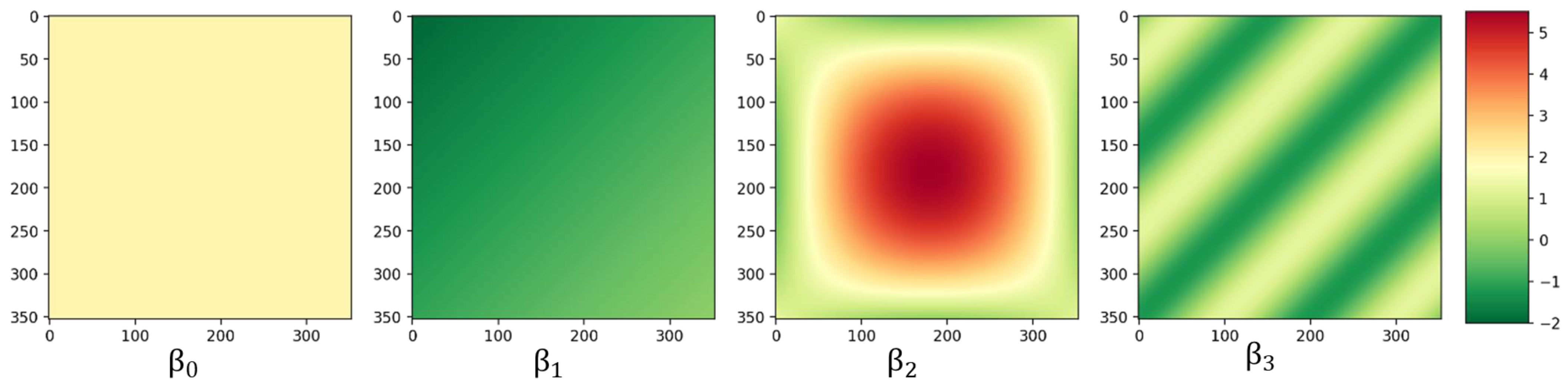
Ijgi 12 00151 g002
Figure 3. True beta coefficient surfaces (Case Scenario 1).
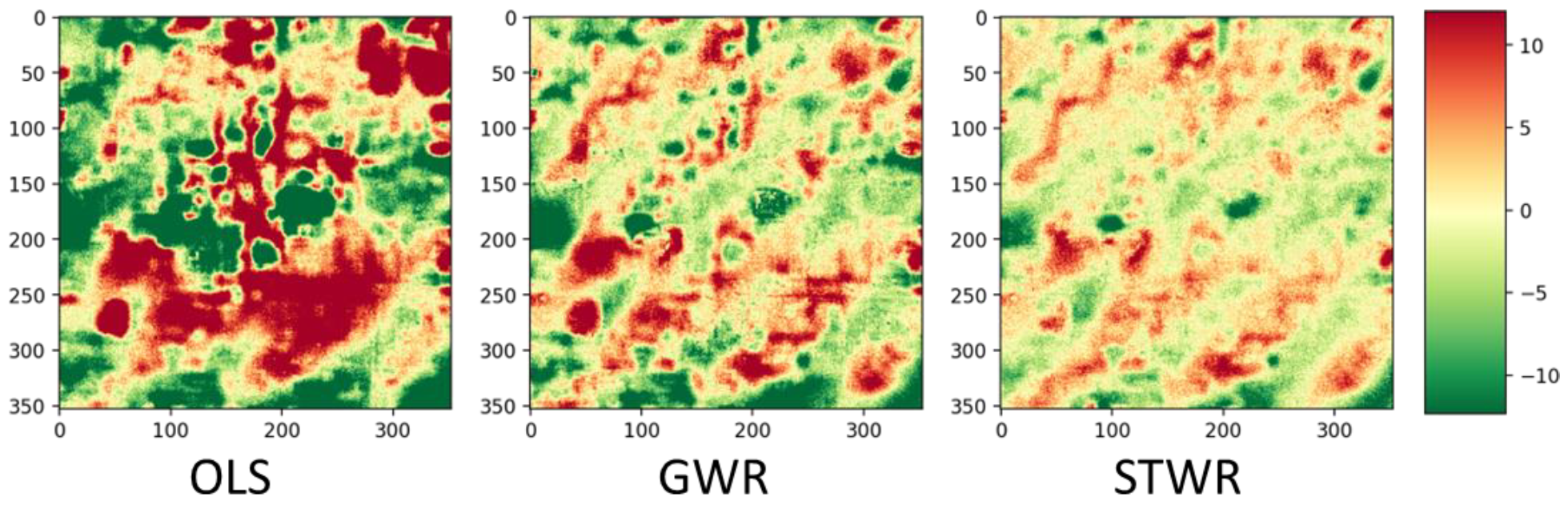
Ijgi 12 00151 g003
Figure 4. Coefficient estimation error surfaces for the OLS, GWR, and STWR models (Case Scenario 1).
Ijgi 12 00151 g004
Figure 5. Response estimation error surfaces for the OLS, GWR, and STWR models (Case Scenario 1).
Ijgi 12 00151 g005
Figure 6. True beta coefficient surfaces (Case Scenario 2).
Ijgi 12 00151 g006
Figure 7. Coefficient estimation error surfaces for the OLS, GWR, and STWR models (Case Scenario 2).
Ijgi 12 00151 g007
Figure 8. Response estimation error surfaces for the OLS, GWR, and STWR models (Case Scenario 2).
Ijgi 12 00151 g008
Figure 9. True beta coefficient surfaces (Case Scenario 3).
Ijgi 12 00151 g009
Figure 10. Coefficient estimation error surfaces for the OLS, GWR, and STWR models (Case Scenario 3).
Ijgi 12 00151 g010
Figure 11. Response estimation error surfaces for the OLS, GWR, and STWR models (Case Scenario 3).
Ijgi 12 00151 g011
Figure 12. Land cover maps of central Phoenix in 2001, 2011, and 2019.
Ijgi 12 00151 g012
Figure 13. Coefficient surface of GNDVI from the STWR model in 2000 (a), 2010 (d), and 2020 (g). Points indicate significant coefficient estimates; (b,e,h) show areas highlighted in the red rectangle; (c,f,i) are Landsat images of the same areas.
Ijgi 12 00151 g013
Figure 14. Coefficient surface of GNDBI from the STWR model in 2000 (a), 2010 (d), and 2020 (g). Points indicate significant coefficient estimates; (b,e,h) show areas highlighted in the red rectangle; (c,f,i) are Landsat images of the same areas.
Ijgi 12 00151 g014
Figure 15. Coefficient surface of LNDVI from the STWR model in 2000 (a), 2010 (d), and 2020 (g). Points indicate significant coefficient estimates; (b,e,h) show areas highlighted in the red rectangle; (c,f,i) are Landsat images of the same areas.
Ijgi 12 00151 g015
Table 1. Mean absolute error scores for beta estimation (Case Scenario 1).
β0β1β2β3
OLS0.2250.0180.0140.102
GWR0.3230.0280.0270.12
STWR0.0840.0130.0080.035
Table 2. MAE and AIC scores for response surfaces generated from the OLS, GWR, and STWR models (Case Scenario 1).
OLSGWRSTWR
MAE3.1973.2323.23
AIC933.443937.549931.836
Table 3. Mean absolute error scores for beta estimation (Case Scenario 2).
β0β1β2β3
OLS7.3831.051.3941.762
GWR4.5740.5890.4882.619
STWR2.0990.2410.2261.264
Table 4. MAE and AIC scores for response surfaces generated from the OLS, GWR, and STWR models (Case Scenario 2).
OLSGWRSTWR
MAE8.7543.5182.188
AIC1290.471041.378844.916
Table 5. Mean absolute error scores for beta estimation (Case Scenario 3).
β0β1β2β3
OLS10.7221.7331.4412.934
GWR7.0271.2020.6283.157
STWR4.8190.4330.4261.718
Table 6. MAE and AIC scores for response surfaces generated from the OLS, GWR, and STWR models (Case Scenario 3).
OLSGWRSTWR
MAE9.9585.3873.597
AIC1349.71163.8681004.234
Table 7. Model goodness-of-fit diagnostic for the OLS, GWR, and STWR models for 2000, 2010, and 2020.
Year200020102020
ModelOLSGWRSTWROLSGWRSTWROLSGWRSTWR
R20.6090.8770.9090.7350.9170.9350.590.9370.948
Table 8. Mean significant coefficient estimates from the STWR model.
GNDVIGNDBILNDVI
2000−0.440.09−1.4
2010−0.280.25−1.2
2020−0.130.43−0.57
Table 9. Mean significant estimates from the STWR by land cover type.
Developed, High IntensityDeveloped,
Medium Intensity
Developed,
Low Intensity
Developed, Open Space
2000GNDVI−0.48−0.44−0.45−0.37
GNDBI0.130.120.140.22
LNDVI−1.37−1.38−1.58−0.89
2010GNDVI−0.1−0.28−0.36−0.37
GNDBI0.130.290.280.5
LNDVI−1.6−0.98−1.28−0.57
2020GNDVI−0.06−0.1−0.13−0.33
GNDBI0.350.530.50.39
LNDVI−0.43−0.5−0.69−0.9
Disclaimer/Publisher’s Note: The statements, opinions and data contained in all publications are solely those of the individual author(s) and contributor(s) and not of MDPI and/or the editor(s). MDPI and/or the editor(s) disclaim responsibility for any injury to people or property resulting from any ideas, methods, instructions or products referred to in the content.

