1. Introduction
Transformation operations are usual in geomatic and geosciences, particularly in mapping and survey fields. Most GIS (Geographical Information Systems) incorporate functions to compute transformation between planar shapes (vector format) and images (raster format). Such transformations depends on the applications requirements and they might involve similarity, affine or projective parameters computation.
Geometrical transformation are also involved in the matching operations which are central issues in computer vision [
1], pattern recognition [
2] and artificial and machine intelligence [
3,
4]. Digital photogrammetry is a field where matching techniques have been studied most intensively—from shape based stereo-matching [
5,
6], to features point-based matching [
7]; particularly interesting are the geometrical transformations applications shown in Reference [
8], which implies an important remark in photogrammetry. Recently some methods based on moment and correlation for measuring shape change have been developed and applied to images [
9,
10].
Nowadays, in Spain, Cadastral and Land Registry administrations are requiring transformation parameters from some surveyed parcels based into an affine transformation, because there are small zones where cadastral parcels have small translation and rotation errors considering the ETRS89-UTM coordinate systems.
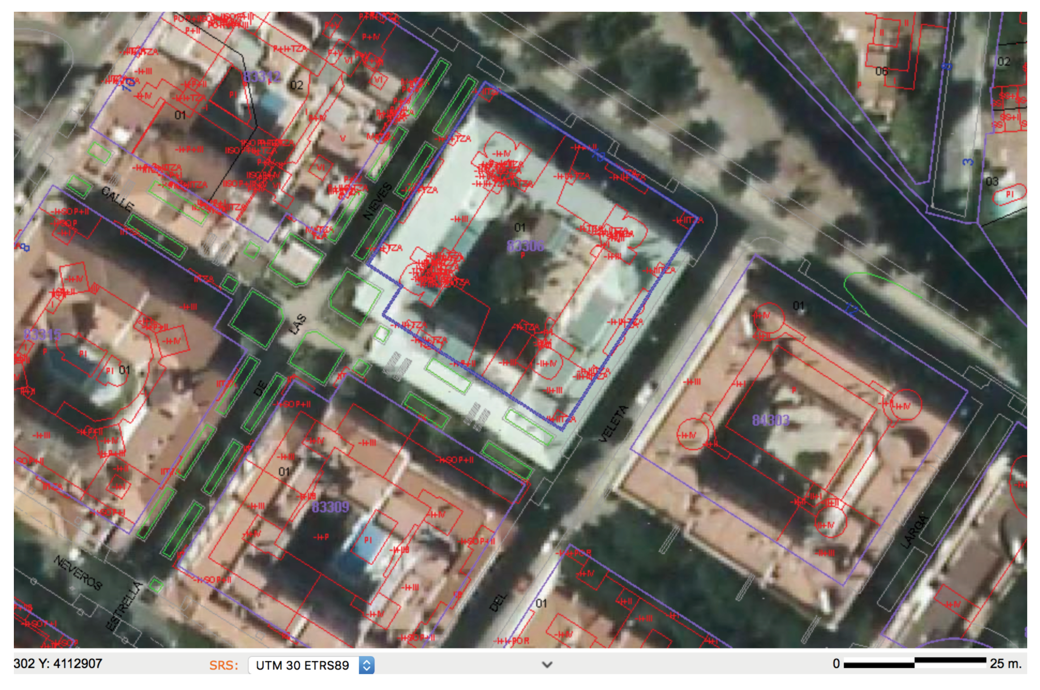
Figure 1 shows an example where there is a displacement between the orthophoto (correctly georeferred) and the corresponding cadastral parcel (vectorial shape in blue color). This small errors could produce legal conflict about the property. For this reason Cadaster and Land Registry consider the reality is the map delineated by a surveyor on the ground who has to compute the transformation parameters between the misregistered cadastral parcel and the on the ground surveyed map.
Most of the above mentioned GIS solutions for transformations require interaction with users, that is, the process is not automated, which implies inefficient and time consuming tasks—the user has to mark corresponding points by hand, in the misregistered and the correct parcel; the number of corresponding points has to be large enough in order to allow a least square solution and consequently knowing the error along the parcel border. Automation has been a constant issue in geosciences and geomatic fields [
11,
12,
13]. It would be interesting to find an algorithm that automatically transformed the corresponding parcels from the erroneous position to the correct one. Several approaches have been carried out in polygon transformation [
6,
14,
15] which could facilitate the automation for cadastral parcel transformation. Particularly interesting is the method from Reference [
6] that is based on the older ones [
16,
17], although the Fourier Descriptors applied to closed curves is described earlier in Reference [
14].
In our study we decided try the methodology from Reference [
6] because it has three main advantages—(a) automation could be absolute (no user interaction is necessary); (b) it is allowed the starting points in the corresponding parcels are not corresponding points and (c) it does not matter the corresponding parcels are composed by a different number of points. The key point in the Hsing and Shenk method is to transform a polygon from the spatial domain to the frequency domain and express such a function by Fourier series. We extend the Hsing and Shenk approach in three aspect—(a) the cadastral application field, (b) the transformation do not change the size from the misregistered parcel, (c) we compute some measures to support making decisions about the best
nth harmonic and number of iterations.
2. Materials and Methods
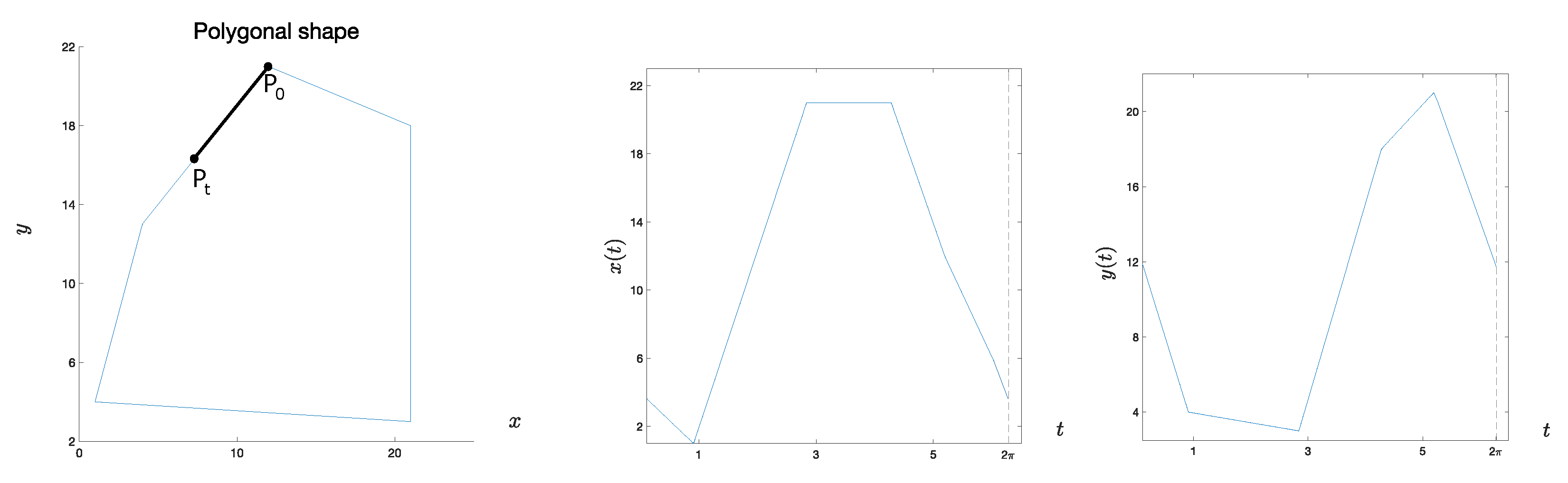
A mapping polygon or a cadastral parcel can be expressed as two periodic functions
and
where
t is defined as
.
L is the total length of the perimeter and
l is the partial distance from a starting point
to an arbitrary point
on the perimeter.
Figure 2 shows a polygonal shape and its representation by the two periodic functions.
The two periodic functions can being formulated by the Fourier descriptors shown in the Equation (
1)
where
Overlapping two corresponding cartographic shapes in an optimal manner could require rotation, translation and scale transformation which could be achieved by similarity, affine or projective transformations. In the case of misregistered cadastral parcels only translations and rotation would be necessary because we assume the following principle—a parcel is almost an exact representation of the real world. Taking into account that the principle of the most suitable transformation between two corresponding shapes represented by their vertices
and
is expressed by Equation (
3) in the spatial domain.
where
The transformation from Equation (
3), in general, does not allow an automated process because of two main reasons:
Nevertheless in the frequency domain, the problem of identifying the corresponding points does not exist; we just need matching the corresponding Fourier descriptors belonging to different harmonics. To compute the harmonics, the polygon vertices should be ordered in the same direction (clockwise or counterclockwise) for both reference and misregistered parcels. Ordered vertices means that two consecutive vertices on the polygon should keep consecutive in the vertices list representing the polygon. The algorithm does not perform correctly if vertices are disordered. The direction condition is easy to automate in case the reference and misregistered polygons are different. The starting point in both the reference and the misregistered polygons could be different to correctly perform the algorithm. Substituting Equation (
1) in Equation (
3) leads us to compute the zero coefficients and the others separately.
Because the
and
are the centroid from the corresponding shapes (see Equation (
2)), the translation computation is straightforward (Equation (
4)):
The rest of the Fourier coefficients can be computed independently for each harmonic because they are orthogonal. Our cadastral parcels do not need to be scaled so that the transformation is limited to a translation (Equation (
4)) and a rotation. For the
nth harmonic the rotation component of the transformation is achieved by Equation (
5).
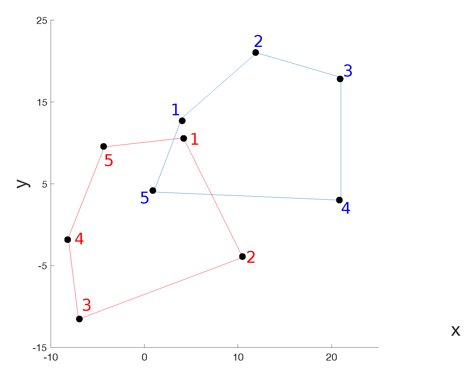
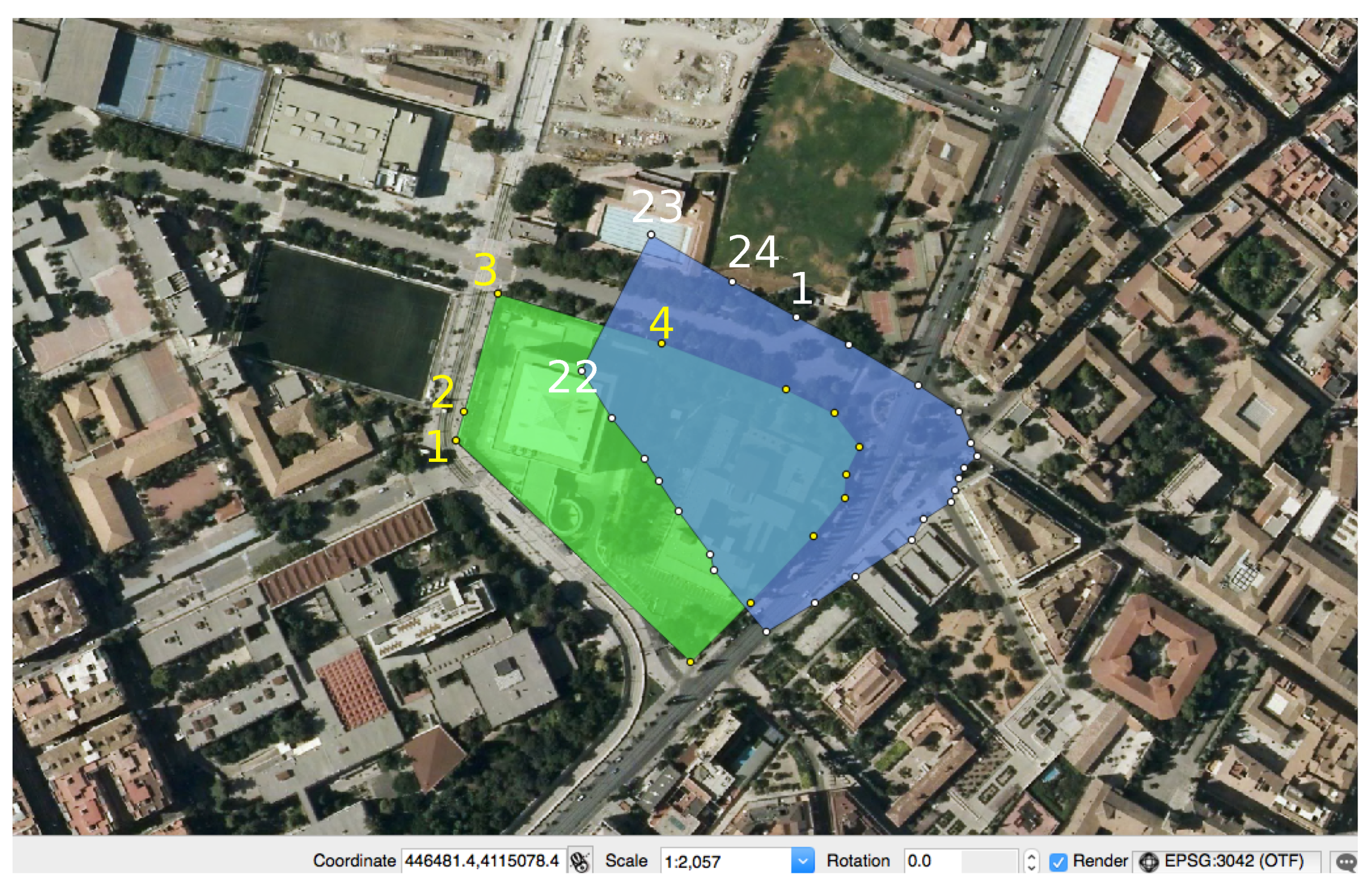
If the starting point of corresponding shapes are not corresponding points, for example, in
Figure 3 the starting point in the blue shape is 1 while the corresponding point in the red shape is approximately the number 4. The consequence is that the Fourier coefficients are different except for the zero coefficients. This is interpreted as a phase shift (
) and the transformation between coefficients taking into account the
is shown in Equation (
6)
The rotation and phase shift combined is expressed by Equation (
7).
At this moment the only unknowns are the rotation angle
and the
and we can solve the unknowns using a least squares approach, where for each harmonic their observations equations have the form of Equation (
8).
In order to use the least squares method we need to linearize the Equation (
8) for each harmonic and compute the first approximations of its coefficients. Such a first approximation can be derived using the harmonic
and
. From Equation (
8), we can denote
and
From Equation (
11) we can compute the initial values for
and
The
A matrix (Equation (
13)) in the least squares solution is a 4 × 2 matrix where odd rows represent the first column and the even rows represent the second column
The
B matrix is
and
where
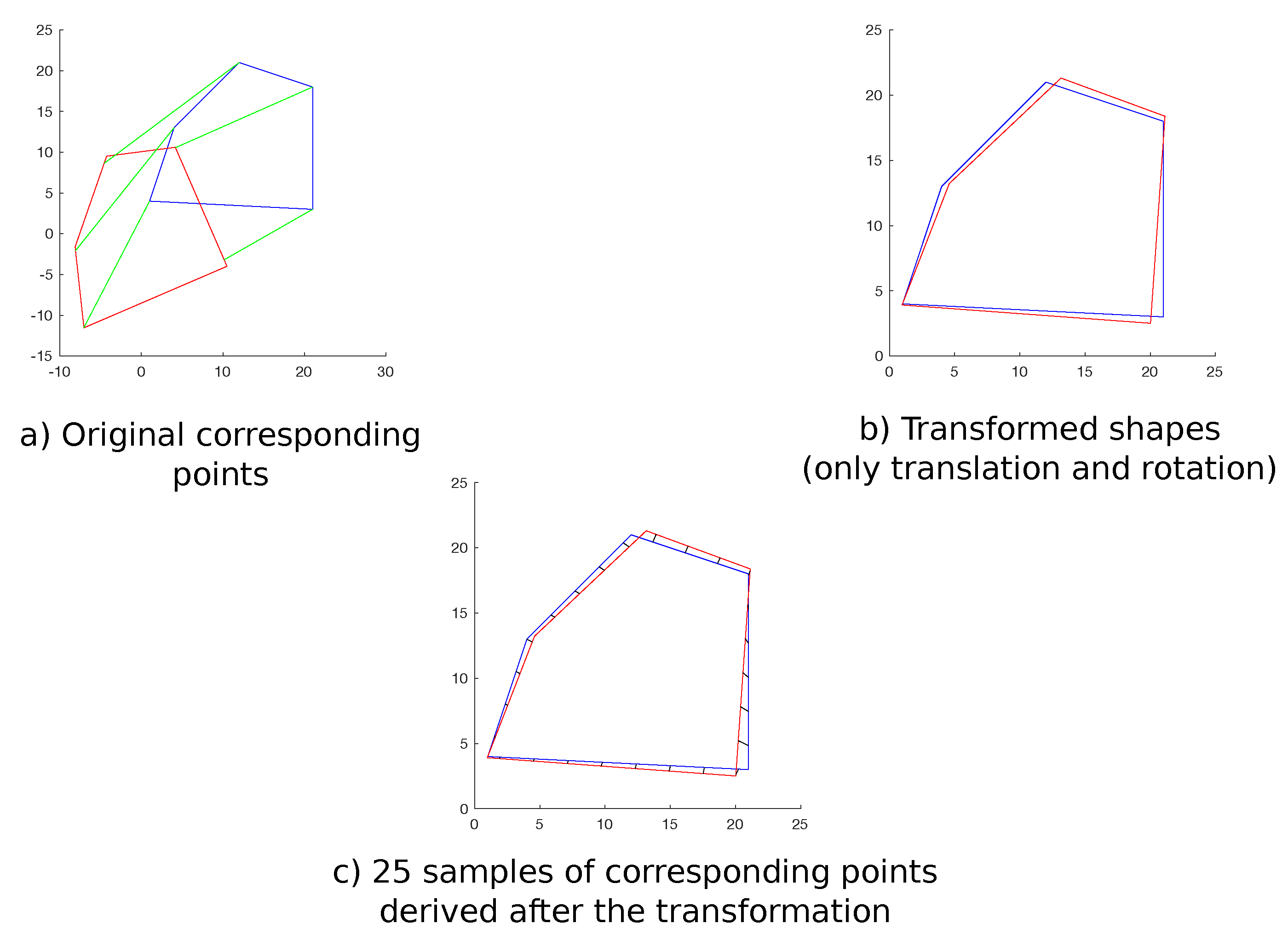
We have programmed the algorithm in Matlab and it requires the points to be ordered in the same direction, although it is allowed that the starting points not to be corresponding points as in
Figure 3—for example, point 1-blue correspond to 4-red. The
Figure 4 shows the result of computing the 4th harmonic and 3 iterations in the least square process (overlapped shapes). We can obtain an approximation of the mean, median and maximum separation between shapes if we compute a large enough sample of separations between shapes.
3. Results and Discussion
We have tested our algorithm on a correct digitized parcel (green in
Figure 5) composed of 12 vertices while the misregistered parcel is composed of 24 vertices (blue in
Figure 5). You can observe that starting points in both parcel are different, so that, we expect a shift phase value
.
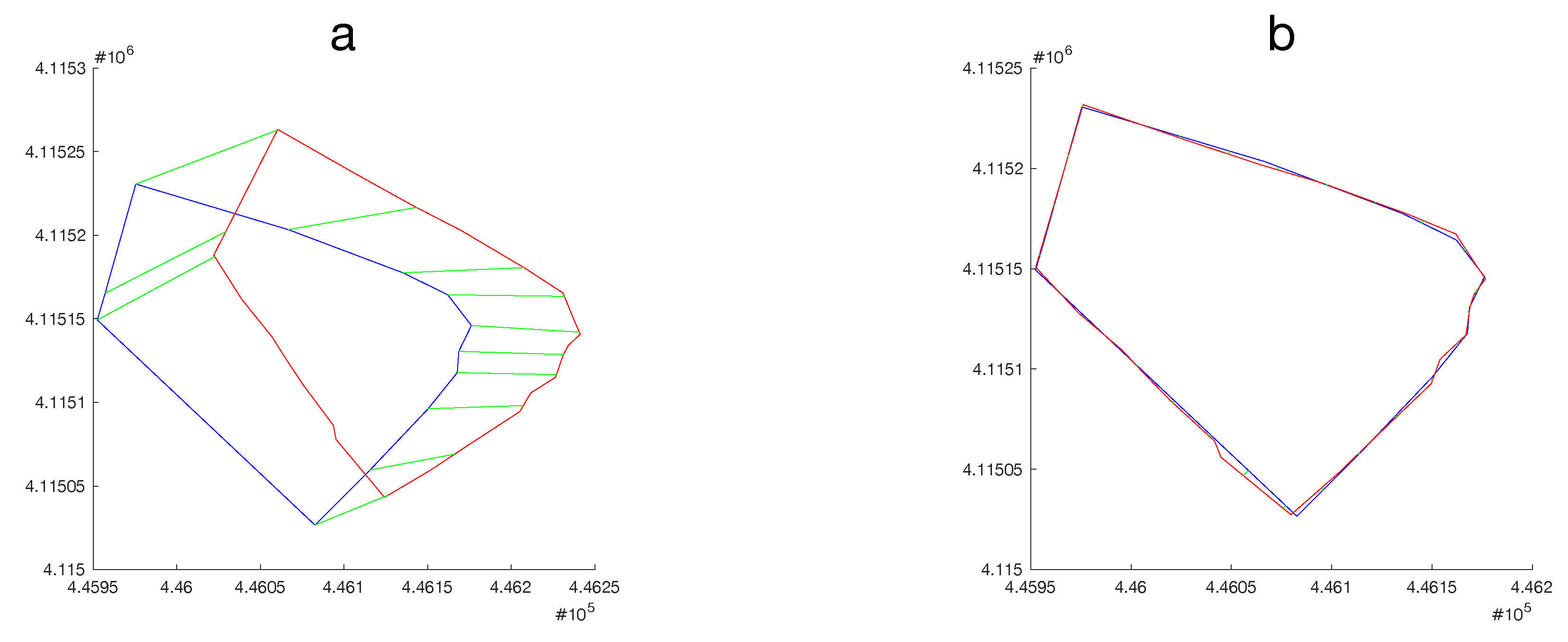
Figure 6a shows the correspondence between the points from the correct parcel (green) to the misregistered one (blue).
Figure 6b shows the transformation applied to the misregistered parcel, so that it overlaps the correct one. The parameters used for the transformation has been the following: 3th harmonic and 3 iterations; and the resulting transformation is described by
and
.
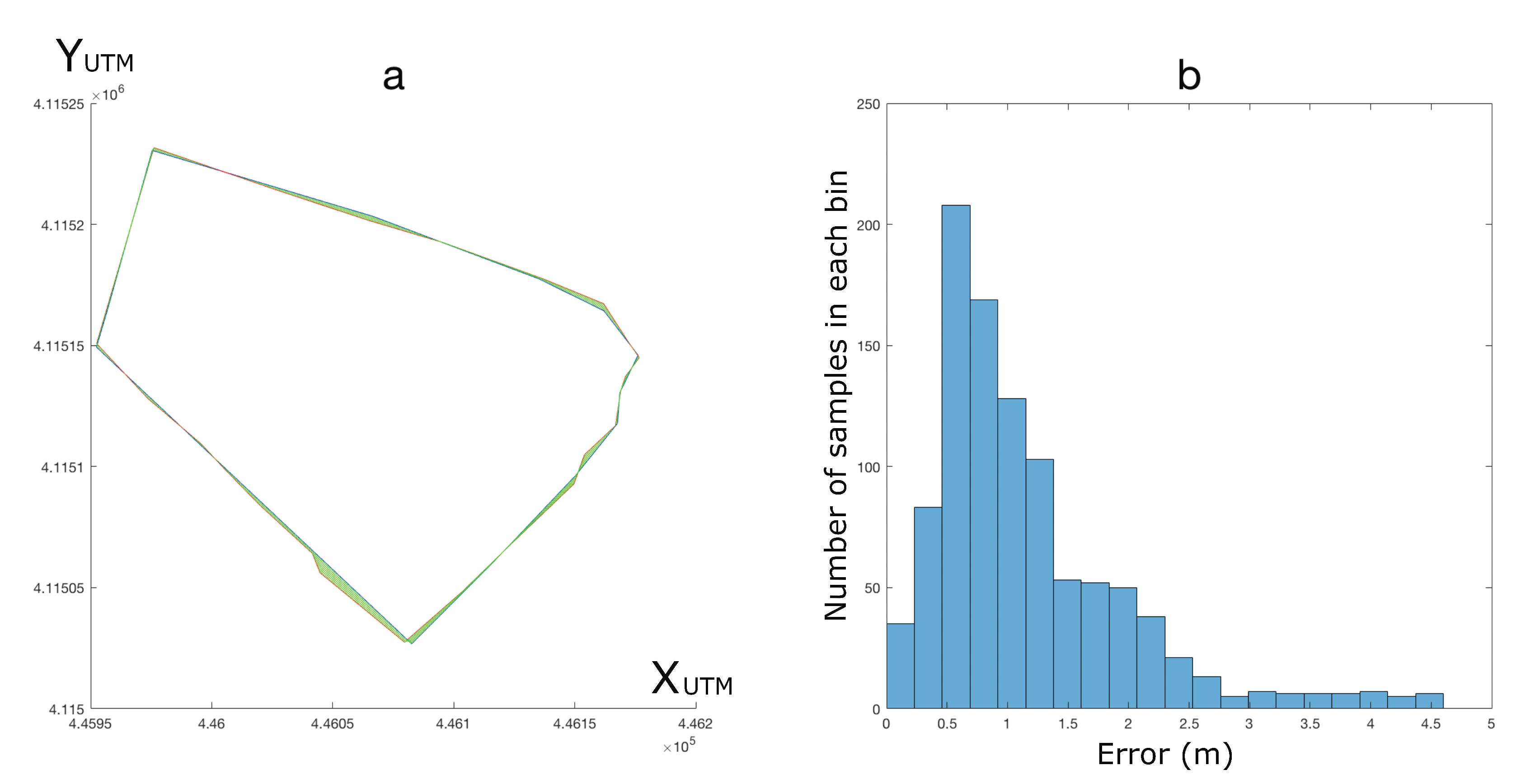
In order to compute the parameters influence on the fitted transformation we have tried different settings of
nth harmonic and iterations numbers and we have computed the corresponding mean, median and maximum separation values between the matched parcels. In order to get a visual information of separation values we have built an histogram for such a measure.
Figure 7a shows the area between parcel after transformation (green color) where separation values are mean (1.169 m), median (0.953 m) and maximum (4.499 m); and
Figure 7b shows the corresponding histogram with 1000 samples distributed into 20 bins. The parameters setting used to obtain
Figure 7 was 2nd harmonic and 2 iterations.
The
Table 1 shows 9 settings (treatment) which combine
nth harmonic and number of iterations. We can observe from
Table 1 the mean separation between corresponding parcels is around 1.7 m and the largest difference between treatment considering the mean value is 2 mm; taking into account that the parcel size is approximately 205 × 130 m, the data seem to indicate there is not a great influence between treatments. If we focus in the maximum separation between corresponding shapes we observe it occurs between 5th harmonic 2 iterations (4.461 m) and the 3rd harmonic 5 iterations (4.529 m), and even in this case the differences is only of 68 mm which is also a small difference.
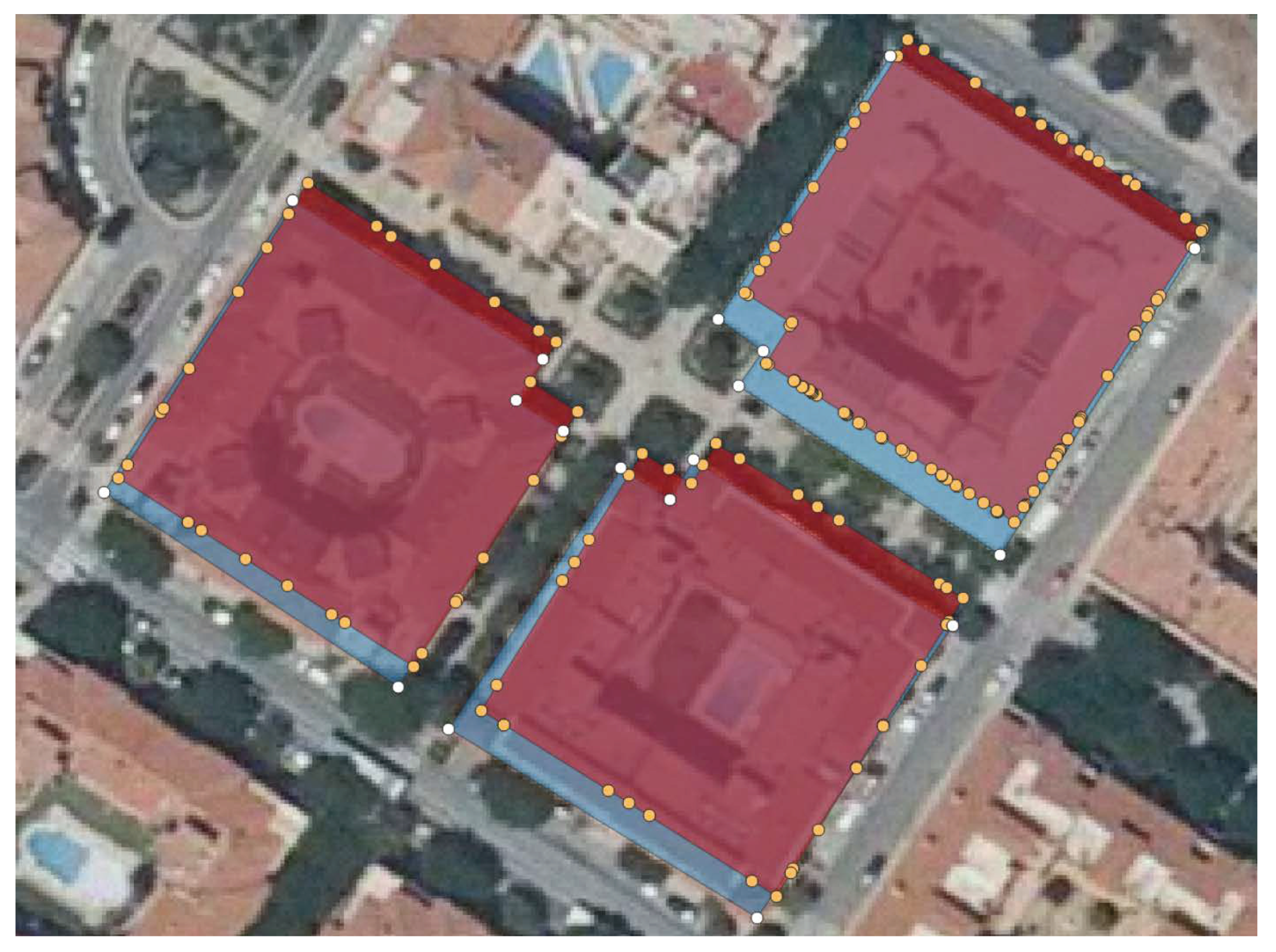
For a more consistent conclusion about the number of harmonic to use in the transformation, we think it is necessary to take into account parcels like those corresponding to buildings. Buildings are the most frequent parcels in urban areas and the most expensive. For this reason an accurate positioning in urban parcels is more important that in countryside ones. A main property in this kind of parcels is that they have both orthogonal and parallel sides. To continue our experiment we have selected three building cadastral parcels that are misregistered, see
Figure 8.
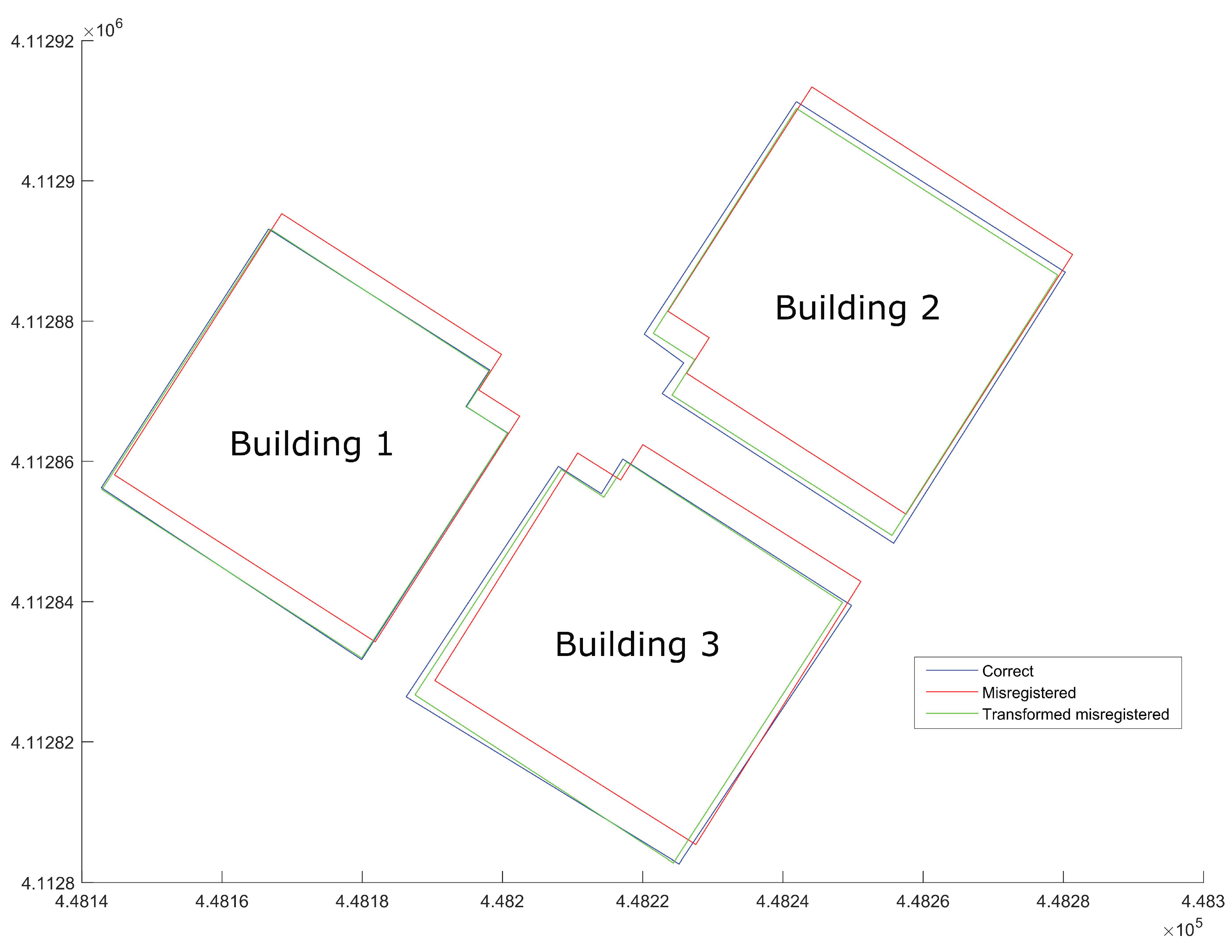
We applied the Fourier-based automatic transformation to the aforementioned three buildings and the graphical result is shown in
Figure 9 where the blue color indicates the correct position for a parcel, the red color refers to the misregistered cadastral parcel and the green polygon is the transformed cadastral parcel after apply the Fourier-based algorithm. For each building we computed the same measures per treatment as in
Table 1, that is, mean, median and maximum. Each treatment is defined by combination of 2 parameters, the
nth harmonic and the number of iterations. The results are shown in
Table 2. From
Figure 9 we can see that the Building 1 is the best fitted, this is because the cadastral parcel and the reference one has approximately the same shape and size; Building 2 keeps the sides parallel but the size is smaller than the reference one; and Building 3 lacks of parallelism in their sides. It seems that geometric features from those buildings explain the results included in
Table 2. We observe that in Building 1 (the more similar between cadastral and reference parcels) there are hardly any differences in the measures when we take into account the
nth harmonic parameter. On the other hand Buildings 2 and 3 have remarkable difference between the 2th and the 3rd harmonic. If we take into account only the number of iterations (N Iter) parameter, the variation in measures is significant from N Iter i to N Iter i + 1 only when the 2th harmonic is fixed; when the 3th or the 5th harmonic is fixed the measures variation is not significant from N Iter i to N Iter i + 1.
According to the previous analysis it seems a reasonable election to use the following parameters: 3rd harmonic and 5 iterations.
4. Conclusions
Transformation operations applied to a mapping shape is a frequent task in geosciences and geomatic fields. In this paper we have focused on the case of two corresponding polygons (representing cadastral parcels), which have small differences in their shapes although they are more or less similar.
Usually transformation parameters referring to similar, affine or projective transformation have been computed identifying corresponding points by hand, which does not imply process automation at all. The main advantage of the Fourier-descriptor-based approach explained in this paper is the whole process automation. We only need to express a polygon in the frequency domain starting from its spatial representation (a list of vertices). Representing a polygon (mapping shape, or cadastral parcel) in the frequency domain has several advantages with respect to its spatial representation in order to compute the transformation parameters—(a) the number of points in the correct shape can be different to the misregistered shape to be transformed; (b) you do not have to match corresponding points between shapes. We applied the Fourier descriptors approach to the mapping shapes used by Cadaster and Land Registry administrations. The correct parcel, usually has been measured by a surveyor, so that we do not want its scale to be changed; therefore the only transformation parameters we need are translation () and rotation ().
We have tried several level of harmonic (from 2nd to ) in order to determine the harmonic level influence in the transformation, and remarkable differences appear in building parcels when non-parallelism and different scales exist between the cadastral and reference parcels. According to our study it seems a reasonable election to use the 3rd harmonic and 5 iterations as parameters for getting the transformation.
The results obtained after automatic transformation, based on Fourier descriptors, show a suitable fit between the corresponding parcels. For this reason it is advisable to use Fourier-descriptors-based transformations by Land Registry and Cadaster administrations when they need parcel transformations.

 ,
, 


