1. Introduction
The manufacturing industry is currently in the midst of the fourth industrial revolution. This digital transformation towards smart manufacturing systems (SMS) is based on the three pillars connectivity, virtualization, and data utilization [
1]. This circumstance is fueled by the rapid development in both information technology (IT) and operational technology (OT), which has led to an increasingly connected and automated world: in essence, a merging of both worlds (IT/OT). Technologies like sensor technology, cloud computing, and AI/big data analytics lead not only to a dramatic increase in the amount of (manufacturing) data, but also to rapidly developing data processing capabilities, which have raised interest in data mining approaches for automating repetitive processes [
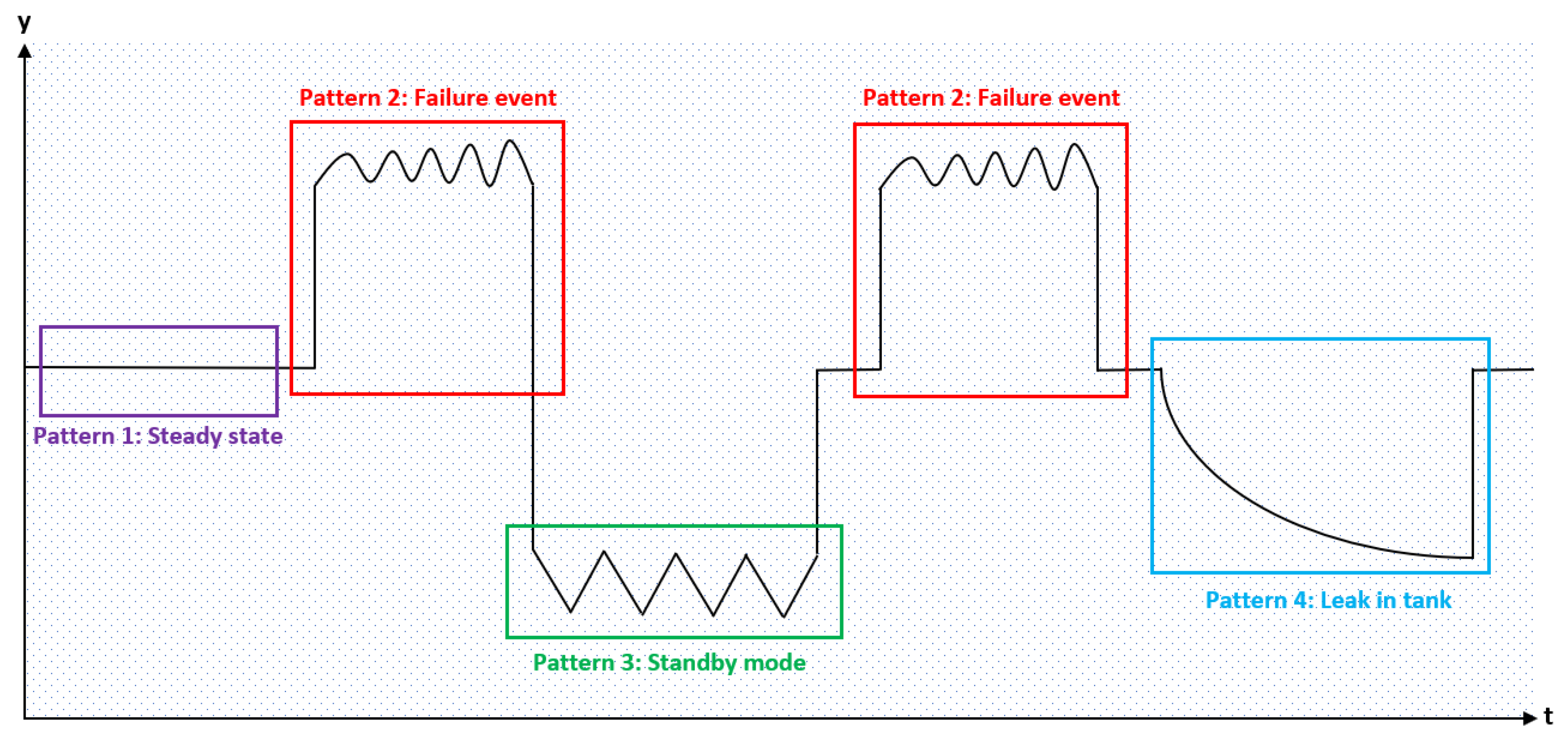
2]. Time series data, thereby, are one of the most common information representation variants in a variety of different business areas. Advanced process monitoring, on which we rely regularly in SMS, typically yields multidimensional data to increase its effectiveness. A specific branch in time series analysis deals with the recognition of reoccurring patterns within the data (see
Figure 1). Time series data analysis generally utilizes established pattern recognition methods in order to identify the steady state, anomalies and characteristic failure patterns. However, the identification of such distinct patterns in multivariate time series represents a highly complex problem due to the interactions (correlation) between variables, time dependency and the usually nonlinear nature of the regarded data [
3,
4]. Furthermore, real-word data are usually noisy and, thus, require pre-processing to become a valuable input for analytical algorithms. Pre-processing enhances the ability of the overall approach to be flexible enough to detect various disturbances, such as missing values, noise or outliers, within the data set, but also sufficiently restrictive so that not all insignificant fluctuations (e.g., measurement errors) are labeled as irregularities. Standard distance-based similarity metrics, which are often used in related unsupervised learning approaches, can therefore not be applied without adaptation for different types of problems [
4,
5].
There is a growing interest in the field of pattern recognition, especially for multivariate time series data due to, on the one hand, increasing availability of potent algorithms and easy-to-use tools, and on the other hand, the realization of the potential valuable impact of insights derived from such data sets. Most of the recent work on clustering, however, focuses on grouping different time series into similar batches [
6,
7]. The paper by [
8] for instance presents a popular approach using fuzzy clustering combined with a dynamic time warping technique resulting in an enhance performance when compared to previous methods. There are only a few authors focusing on pattern recognition within a single time series, such as we regularly are confronted in maintenance applications [
4].
This paper presents a framework to utilize multivariate data to identify reoccurring patterns in real-world manufacturing data. The objective is to identify failure patterns for new applications in the area of maintenance.
We analyze the drying process of plastic granulate in an industrial drying hopper equipped with multiple sensors. The number of different failure patterns (sources for defects) is not known beforehand and the sensor readings are subject to natural fluctuations (noise). The overall work presented in this manuscript includes a comparison of two different approaches towards the identification of unique patterns in the data set. One processing path includes the sequential use of common segmentation and clustering algorithms to identify patterns, which might lead to a better respective (both steps of the chain) and, therefore, overall performance. The second approach features a collaborative method with a built-in time dependency structure, thereby avoiding a multiplication of losses due to a sequential processing chain. The better performing method is fine-tuned afterwards in terms of its hyperparameters. The resulting patterns (clusters) that are identified by the framework can then serve as input for advanced monitoring methods predicting upcoming failures and ultimately reducing unplanned machine downtime in the future.
The outline of this paper features a short introduction to the topic of plastic granulate drying and time series clustering in
Section 2, followed by the proposed framework in
Section 3. Finally, the results are presented in
Section 4 and consequently discussed in
Section 5.
2. State of the Art
Industry 4.0, machine learning, and artificial intelligence (AI) are popular topics in the current scientific discourse and, therefore, the current state of the art is subject to frequent changes or newly arising theories and topics [
1]. Thus, we chose to apply the Grounded Theory Approach, originally developed by Glaser and Strauss in 1967 [
9], to gather and subsequently analyze the existing knowledge on the topic of pattern recognition on time series data in the context of Smart Manufacturing Systems (SMS). The approach encourages inductive reasoning for the formulation of the experimental setup and, hence, fosters the development of a practical state of the art framework [
10]. The corresponding literature was selected from the results of a search term optimization identifying comparable research approaches and problems. We used established academic research databases, in particular Scopus, Web of Science, IEEE Xplore, and ScienceDirect, to execute the keyword-based literature search process. The most relevant papers were selected according to their degree of relation to subject of patter recognition in time series for SMS.
In order to establish an automated event detection method for SMS through an unsupervised machine learning framework, we need to take a closer look at the data and its underlying manufacturing process. Domain knowledge is key to developing successful machine learning applications in a manufacturing context. Data mining process phases, such as feature extraction and the selection of suitable algorithms and machine learning models, benefit form process understanding and the appropriate application of these insights [
4]. The following chapter introduces the general drying process of plastic granulates and presents respective data usable for the analysis.
2.1. Manufacturing Process
Drying hoppers are industrial machines, which are mostly used to dry and remove moisture from non-hygroscopic and slightly hygroscopic plastic pellets. They are especially effective for the process of drying the surface area of non-hygroscopic resin pellets prior to further fabrication [
11] to avoid quality issues further down the process chain such as voids caused by gasification of moisture in the final parts. The drying process in general is a vital step in the chain of manufacturing for diverse types of polymers since the excess moisture will otherwise react during the melting process. This might result in a loss of molecular weight and subsequently to changes in regard of the physical properties, such as reduced tensile and impact strength of the material [
12,
13].
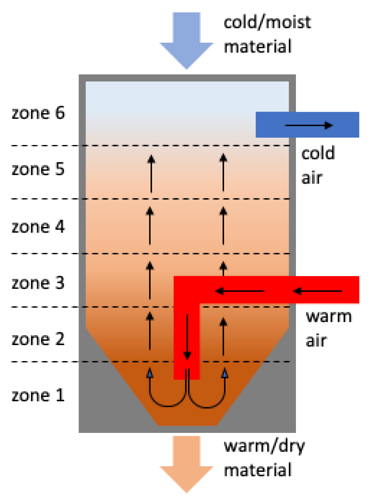
Thereby, most of the modern drying hoppers are structured similarly, in order to ensure an even temperature distribution while also maintaining an even mass material flow. They feature a vertically cylindric body with a conical hole at the bottom, as depicted in
Figure 2. The spreader tubes inside the hopper then inject hot and dry air into the chamber, while the granulate is slowly moving from the top to the bottom valve [
11,
13].
After the hot air has passed the material, it is cleared, dried, (re-)heated (if necessary) and then again reinjected into the drying chamber. For a drying process to be successful in achieving the targeted humidity, there are three major factors that need to be considered: Drying time, drying temperature, and the dryness of the circulating air [
13]. The most intuitive factor might be the drying time since the circulating air can only take a certain amount of humidity from the material until it is saturated. The specific amount of time that the material needs to stay in the machine in order to achieve a defined humidity can be calculated as a function of air temperature, input dryness of the material and target humidity. In general, the drying process has a concave form insofar as the percentage humidity reduction is steep and flattens during later stages [
12,
14]. Both air dryness and temperature also play decisive roles for the drying process and are usually coordinated in dependency of one another. By drying the air, the relative humidity is reduced and consequently the moisture holding capacity increases, whereas a higher temperature speeds up the drying process, since it facilitates the diffusion of water from the interior to the surface of the material [
11,
14]. However, there might be adverse effects of too high temperatures on materials quality depending on the plastic itself that need to be considered.
Due to the critical implications of a malfunctioning drying hopper system, the corresponding process is usually monitored round the clock. In our use case, a six-zoned temperature probe for the monitoring process, which continuously measures the temperature at different locations (heights) of the vertically aligned drying chamber (see
Figure 1), is applied. Doing so facilitates the indirect detection of a variety of different reoccurring disruptions in the drying process, such as over- or under-dried material, heater malfunctions, and many more since most of those incidents are directly connected or at least can be derived indirectly from the temperature of the circulating air [
13]. This is also the reason why these six temperature zones play a major role in determining the performances of the different pattern recognition approaches presented in this paper.
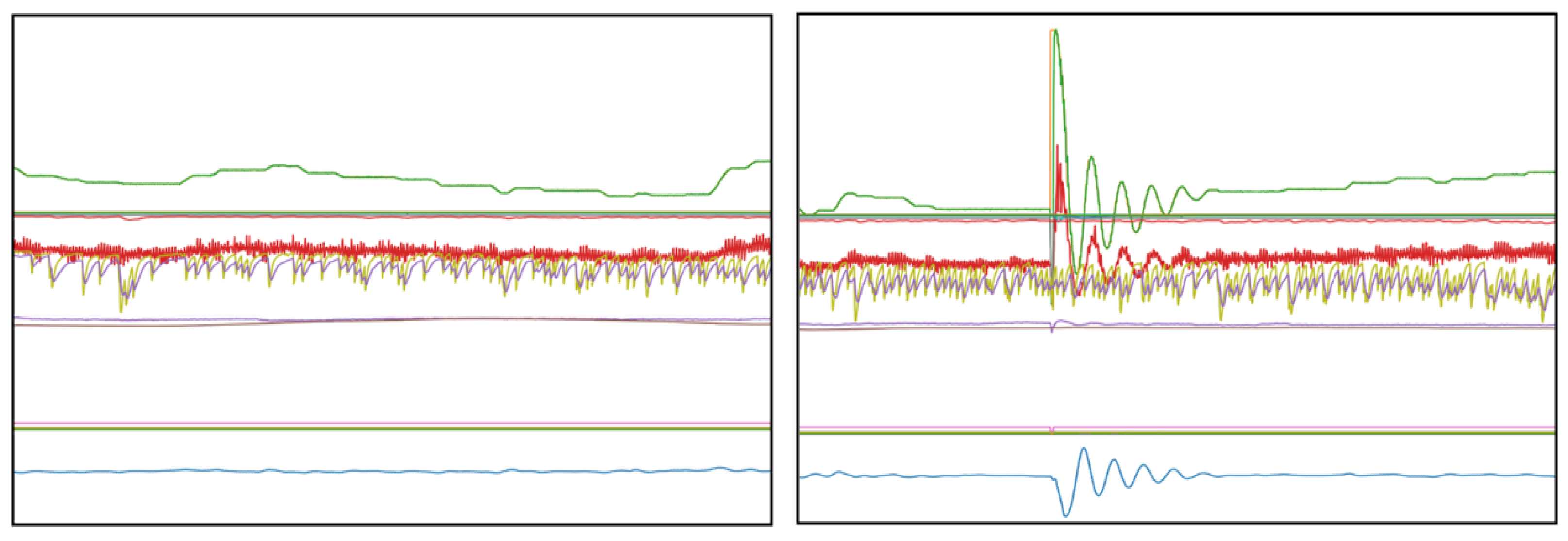
The data set used for this analysis is based on two separate data sources, two individually controlled, yet identical, drying hopper machines located in the same manufacturing plant. Each drying hopper was monitored over a specific time, 6 months for machine one (M1) and 4 months for machine two (M2), whereby an automatic reading of the sensor output was conducted every 60 s over the entire monitoring period. In addition to the different temperature zones, the data set contains a variety of other operational process related sensor data. After the initial preprocessing of the data set, which involves the removal of missing, damaged, and severely fragmented data objects, the resulting data set consists of 31 (M1) and 37 (M2) different features and 263,479 (M1) and 176,703 (M2) instances. The signals from the sensors are partly continuous, such as the real time temperature measurements of the circulating air or panel, as well as partly binary for information on the status of different components such as heater or blower (on/off). The following
Figure 3 illustrates the different events involved, by displaying the steady state of the machine (left) in comparison to a typical disruption (right).
2.2. Analytical Approaches
There is a plethora of scientific work available focused on the topic of time series analysis, in particular within the last decades. Two major themes among the published research that are strongly related to the practical application of those algorithms are (i) fault (anomaly) detection within time series and (ii) clustering of different time series [
4]. Since both of these areas are comparably well developed evidenced by the large amount of available scientific contributions, some pattern recognition approaches employed this to construct a pipeline-like processing framework to cluster time series data. The works [
15,
16,
17] are comprehensive reviews and applications focused on this topical area and used segmentation and clustering methods subsequently. The majority of these papers apply correlation analysis, wavelet transformation, and principle component analysis (PCA) based metrics to identify homogeneous segments and to assign the data points to each cluster. Classical distance-based metrics (e.g., Euclidean distance) are still used in various scientific works today, most often to provide a benchmark for the evaluation process [
4,
5]. A more recent work by [
8] presented an approach using fuzzy clustering combined with a dynamic time warping technique to identify the different clusters after the segmentation has been completed.
Another reoccurring theme in the field of pattern recognition in times series is the domain those approaches are applied mostly. The majority of datasets that has been used to evaluate theoretical frameworks stem from the medical domain (e.g., ECG and biological signals), the financial sector (e.g., exchange rates and stock trade), and speech recognition applications [
3,
4,
5]. Significantly fewer works focus on manufacturing applications and the analysis of industrial machines (e.g., gas turbine and water level monitoring), especially in a maintenance context [
4]. Most recent contributions to the maintenance discourse focus on the prediction and classification of previously defined failure patterns, thereby solely relying on the preceding groundwork of experts.
Hence, the use of time series analysis in SMS itself provides a multitude of opportunities for further research. Additionally, the effectiveness of cutting-edge event detection methods is examined for industrial applications, which later can be used to assist or even replace expert centered error recognition systems. Most importantly, the adaption and usage of advanced pattern recognition algorithms for SMS serves as a stepping stone into further studies combining domain expertise and novel machine learning algorithms for solving advanced industrial problems, therefore moving towards a more automated data processing chain overall.
To achieve this goal, this paper aims to combine the best of both worlds: the latest findings from the general time series analysis literature as well as complex, real-world industrial data to put those cutting-edge approaches to the test. In doing so, we also use feature fusion [
4] and sequential pattern recognition methods [
18], which have been successfully applied previously within an industrial context. However, an important distinction to comparable works in this field is that we start without any prior expert knowledge on the characteristics (e.g., type, frequency, and shape) of the failure patterns. Furthermore, we also chose a quantitative method to compare competing time series analysis approaches by implementing various methods in combination of different cost function, while comparable papers often select promising configurations beforehand without further examination. This rigorous (in-depth) proceeding, however, results in a trade-off so that only a limited number of different algorithms (or rather pathways) could be implemented in the scope of this scientific work, which is admittedly smaller than comparable studies, such as [
19,
20] produced.
3. Research Methodology
An overview of the novel framework proposed in this paper is illustrated in
Figure 4. It is important to note that it includes two separate approaches to pattern recognition that were conducted separately and then compared to identify the superior process given the unique characteristics of the data set. This is intentionally included in the framework as data sets differ significantly in their nature and providing options to the user that allow to compare the performance as part of the framework is a promising way of leveraging these differences in data sets today.
3.1. Principle Component Analysis (PCA)
The first step, after generally checking and cleaning the data (pre-processing), involves a PCA to identify irrelevant features to reduce the dimensionality (feature reduction) and therefore overall complexity of the data set. In doing so, the implemented algorithm is successively constructing “artificial variables” (principle components) as linear combination of the original variables, so that those new vectors are orthogonally aligned to each other. This new representation of the data with linear independent vectors can subsequently be used, instead of the singular vectors, as input data for the affiliated analysis processes (segmentation and clustering) [
4]. After the data has been cleared and rearranged, we can start with the first step (of the first pathway) of segmenting the time series.
3.2. Heuristic Segmentation
Following the first branch of the pattern recognition pathway, we consider the multivariate signal
with
being a m-dimensional (number of sensors) observation.
. stands for the total number of observations and
is the index of the measurements in time. Consequently, the multivariate time series can also be expressed as the following
matrix:
In order to identify sections of the time series with similar trajectories (patterns), we first need to partition the signal into internal homogeneous segments. Ideally, the time series will be automatically split into segments representing (i) regular machine behavior (steady state) on the one side and (ii) segments with a variety of events (including failure events) on the other side as the final output.
An event or segment in this case can therefore be formulated as , with being the overall segment of the partition and with denoting the length and location of the interval. For a less formal notation, it can also be denoted as . The points , in which the state of the signal changes, are usually referred to as change points or break points and are given as with being the chronologically first break point in the time series. The set of true break points, which was acquired by manually labeling the time series, is denoted as with its corresponding elements , while is used to record the approximated break points retuned by the algorithm.
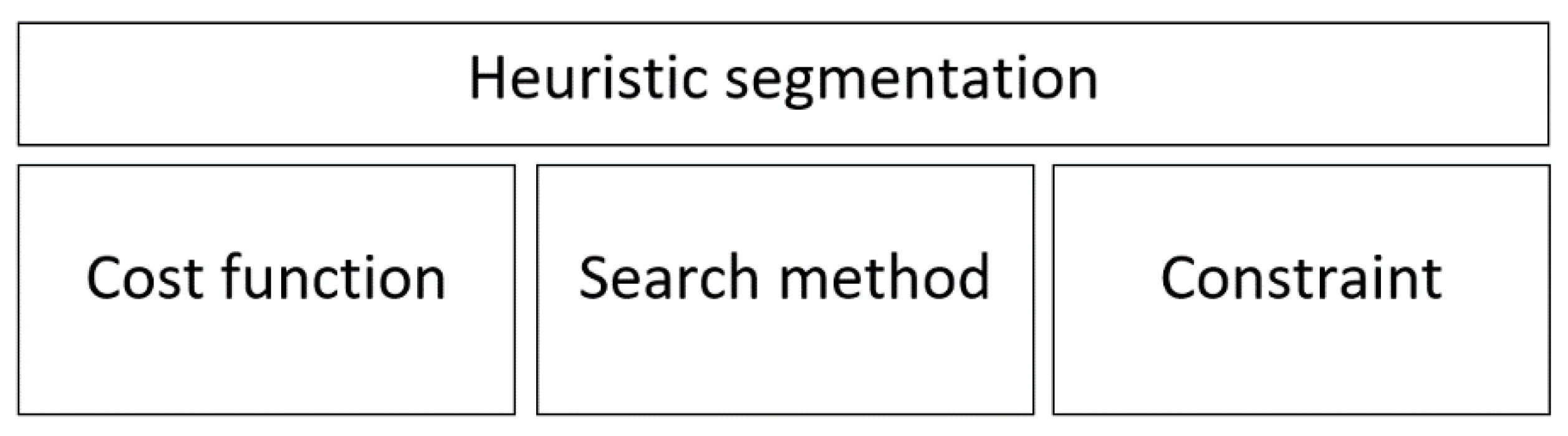
To solve this problem, we will apply the heuristic changepoint detection method implemented in a package called ruptures [
5], which can be described as a combination of three defining elements: cost function, search method, and (penalty) constraint (see
Figure 5).
Formally the change point detection (segmentation) can be viewed as model selection problem, which tries to choose the best possible partition of the time series given a quantitative criterion. This criterion is most often expressed through the form of cost functions and is therefore denoted as
, which needs to be minimized during this process of optimization [
5]. In fact, the criterion function consists of a sum of costs of all segments that define the segmentation:
For this formulation we also need to define the dummy indices
as the first index and
as the end of the time series. Furthermore, we need to introduce a penalty function for our overall minimization problem, since the algorithm would otherwise always converge to an oversegmentation, where all points are ultimately represented in their own individual segment and therefore minimizing the overall sum of costs [
5]. The final optimization problem for the segmentation is therefore given by:
The penalty function (constraint) can also be interpreted as complexity measure for the segmentation and needs to be adjusted for each heuristic, respectively. In this case we choose a linear penalty function given by
with
. Choosing a linear penalty function thereby aligns with successful implementations from recent literature [
5,
21,
22,
23] and with well-known model selection criterions such as the Akaike’s information criterion and the Bayesian information criterion.
After our problem has been defined, we need to choose a search method to calculate the break points of the time series. There are a variety of different solving algorithms available from which we will explore three approaches (also featured in ruptures) in more depth in the following section.
3.2.1. Sliding Window Segmentation
The core idea of the sliding window algorithm is to approach the partitioning (segmentation) problem by moving a fix sized window over the time series. The window basically represents the area of vision or rather area of focus of the algorithm for a given iteration [
6]. Thereby, the approach implemented by ruptures is not directly dividing the times series in each iteration solely based on the information given in the window, but rather by calculating a so-called discrepancy measure for each point in the signal. To do so, the window is split in two parts (“left” and “right”) along its center point [
5]. The discrepancy measure is defined as following:
Given a cost function
and interval
, the discrepancy measure is basically computing the difference in cost between treating the sub-signal
as one segment in comparison to splitting the interval up into two separate segments (
and
) at point
. Consequently, the discrepancy function is reaching high values when the two sub-windows contain dissimilar segments according to the cost function. After the values of the discrepancy function have been computed for all points of the time series, the algorithm analyses the discrepancy curve to identify the maximum values (peak search). The peaks of the function correspond to the incidents, in which the window was holding two highly dissimilar segments in each sub-window and therefore gives us the break points of the signal [
5].
Figure 6 provides a schematic overview of the algorithm to provide more clarification of its functionality and objective.
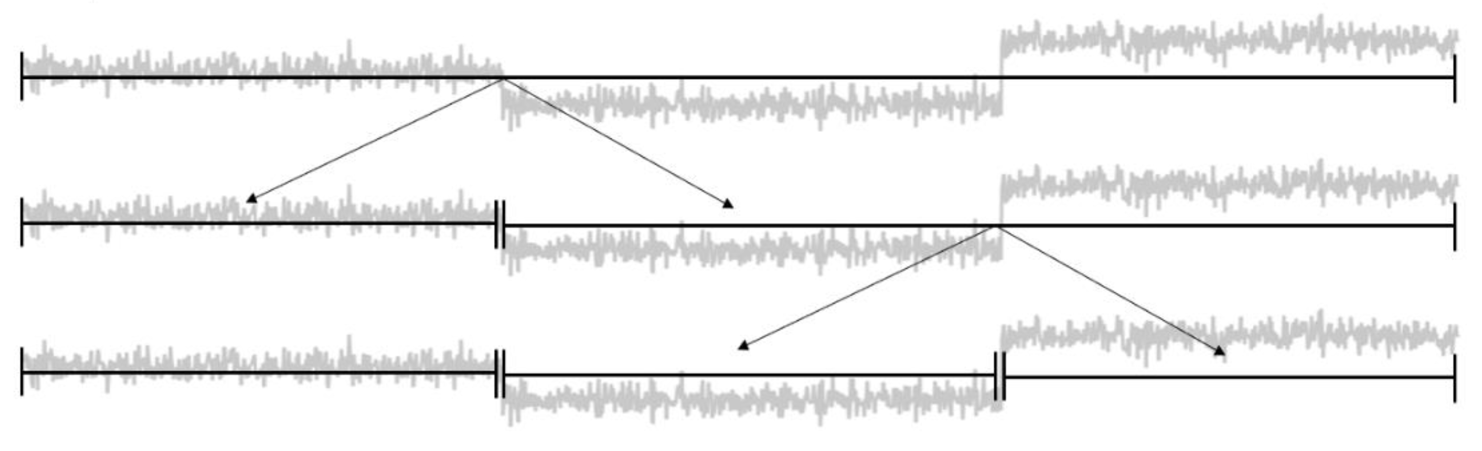
3.2.2. Top-Down Segmentation
The top-down method is a greedy-like approach to partition the time series iteratively. To do so, it considers the whole time series and calculates the total cost for each possible binary segmentation of the signal at first. After the most cost-efficient partitioning has been found, the time series is split at the identified change point and the procedure repeats for each sub-signal, respectively [
5,
6]. The calculation on which the partitioning decision of each stage of the iterative algorithm is based on can be easily displayed with the following formula:
It represents the decision mechanism for the first iteration of the algorithm. However, it can be applied to each sub-signal after the initial time series has been divided initially. The stopping criterion of the approach depends entirely on the previously defined penalty function of the overall problem (2). Thereby, the cost-savior of each partitioning is compared to the penalty of introducing another break point to the existing set of change points. The algorithm terminates when there is no partitioning within the iteration that has a higher cost-savior compared to the penalty value [
5]. The schematic depiction in
Figure 7 provides an overview over the whole process.
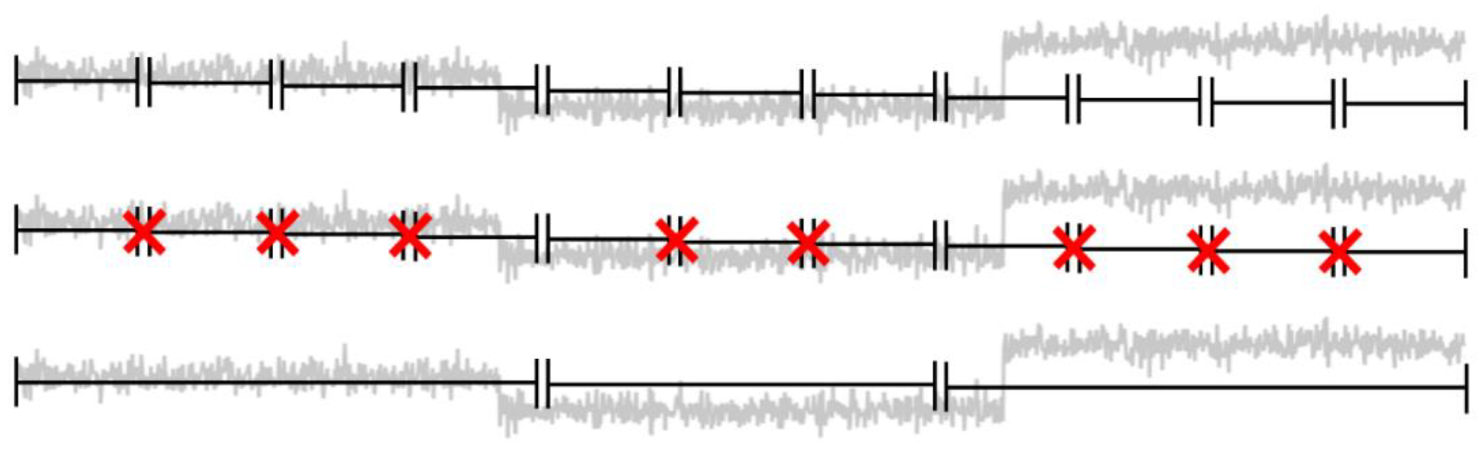
3.2.3. Bottom-Up Segmentation
The bottom-up segmentation can be best described as the counterpart to the previously discussed top-down approach. Herby, the start of the algorithm is characterized by the creation of a fine, evenly distributed partitioning (all segments have the same length) of the entire time series. Subsequently, the algorithm merges the most cost-efficient pair of adjacent segments in a greedy-like fashion [
5,
6]. To clarify the overall process, a schematic overview of the process is depicted in
Figure 8.
In contrast to other bottom-up methods covered in the current literature on segmentation [
6], the approach we used in this case also harnesses the discrepancy measure defined above (see sliding window) in order to determine the most cost-efficient pairs to merge. During each iteration, all temporary change points are ranked according to the discrepancy measure, which takes into account all of the points in both adjacent segments. Consequently, the break point with the lowest discrepancy measure is deleted from the set of potential break points. This process continuous until the increase in costs, due to the removal of a break point, cannot be compensated by the reduction of the penalty and the algorithm terminates [
5].
After completing the heuristic segmentation, standard clustering approaches such as k-means or Gaussian mixture models can be applied (in combination with DTW) to sort the time series snippets into equal groups [
8]. These approaches work similarly to parts of the TICC algorithm and are therefore relevant to the depictions in the following chapter as indicated by the ‘*’ in
Figure 4.
3.3. Toeplitz inverse-Covariance Clustering (TICC)
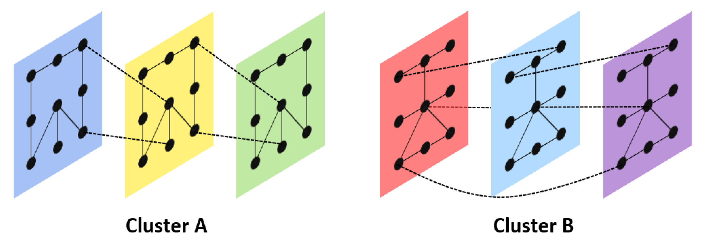
In contrary to the heuristic approaches that start by partitioning the signal first and then conduct the clustering, the alternative method we explored to tackle the problem includes the algorithm TICC, which approaches the problem by simultaneously segmenting and clustering the multivariate time series through the use of Markov random fields (MRF). The reason for using Markov networks is that they denote relationships between variables generally much stronger than more simple correlation-based models. Thereby, each cluster is defined as a dependency network, which is taking into account both the interdependencies of all dimensions (features) of an observation
and the dependency to near neighbor point
. Each cluster network can be described as a multilayer undirected graph, were the vertices are representing the random variables and the edges indicate a certain dependency among them [
3]. The layers of each network correspond to the number of consecutive observations (instances) and therefore to the receptive field of the model (see
Figure 9).
Another important differentiating quality of MRFs is that, under certain criteria, they can be used to mimic a multivariate Gaussian model with respect to the graphical representation of the multivariate distribution. Since this applies in our case, we can use the precision matrix (inverse covariance matrix) as a formal representation of the graphical structure, where a zero (conditional independence) in the matrix corresponds to a missing edge between two variables. The benefits of using the precision matrix
over the covariance matrix are manifold and include computational advantages as the result of a tendency of being sparse. Furthermore, the sparsity of the MRFs also prevents overfitting and therefore increase the robustness of the overall approach [
3,
24].
3.3.1. Problem Formulation
In addition to the preciously established notation, we need to introduce a few modifications for the formulation of the TICC problem. First, we are interested in a short subsequence (with ), rather than just one point in time . Therefore, to assign the data points to the corresponding clusters, we need to address those points as dimensional vectors . The number of clusters, which has to be defined beforehand, will be denoted as and the time horizon of the short subsequence will be set by the window size .
A challenge of the TICC approach is to address the assignment problem of matching the data points to one of the
clusters and thus determining the assignment sets
with
. Furthermore, the algorithm must update the cluster parameters
based on the previously calculated assignment mappings [
3]. The overall optimization problem can be formulated as:
This entire problem is called Toeplitz inverse covariance-based clustering (TICC).
in the formula reflects the set of symmetric block Toeplitz
matrices, which adds an additional constraint for the construction of the MRFs. The enforced structure ensures the time-invariant property of each cluster so that the cluster assignments do not depend on gate-events. This implies that any edge between two layers
and
must also exist for the layers
and
. The first expression
represents an additional sparsity constraint based on the Hadamard product of the inverse covariance matrix with the regularization parameter
. The second part of the formula
states the core optimization problem of cluster parameter fitting, given assignment set
(log likelihood). The last part of the overall problem addresses the desired property of temporal consistency. By adding a penalty
for each time that two consecutive observations are assigned to two different cluster
, the overall algorithm is incentivized to hold those instances to a minimum [
3].
The method to handle this complex problem can be described as a variation of the expectation maximization (EM) algorithm, which is commonly used to solve related clustering issues by applying Gaussian Mixture Models [
25].
3.3.2. Cluster assignment (Expectation)
Similar to the expectation step in the common EM algorithm, TICC starts with the assignment of observations to the given clusters. However, to begin this process we need a prior distribution to which the data points can be assigned to. Hence, the overall TICC algorithm is initialized by conducting a k-means clustering to calculate the initial cluster parameters
. After the initialization phase, the points are assigned to the most suitable cluster by fixing the values of the precision matrix
[
3]. This leaves us with the following combinatorial optimization problem for
:
The sparsity constraint is not directly relevant for this step since the shape of the precision matrix
is automatically fixed with its values. Thus, the resulting constant term of the Hadamard product can be neglected. Each of the short subsequences
is therefore primarily assigned to a cluster
based on its maximum likelihood under the regard of temporal consistency (minimize number of “break points”). The problem (6) is subsequently solved by harnessing the dynamic programming approach of the Viterbi algorithm [
26]. The problem is translated into a graphical representation (
Figure 10), which represents each decision (per instance) the algorithm can make to assign the data points consecutively [
3].
Subsequently, the Viterbi algorithm is returning the minimum cost path (Viterbi path) by calculating the total cost values of each vertex recursively while remembering the minimum cost path simultaneously [
26].
3.3.3. Updating Cluster Parameters (Maximization)
The maximization step of the EM algorithm concerns the updating of the inverse covariance matrices of the clusters once the assignments of the E-step have been given. For this step, the assignment sets
are frozen and the precision matrices
are adjusted based on the corresponding observations. Similar to the assignment problem before, the overall TICC problem (5) can be simplified for this step, since the temporal consistency is strongly tied to the assignment of the datapoints. As seen before, the whole term can therefore be dropped while solving the newly arising subproblem (7), which is expressed in the following formula [
3]:
Another relevant property of this optimization function is that the updating problem for each cluster can be calculated independently since there is no reliance on previous or cross-connected results of other clusters as in problem (6). Therefore, all updates can be done in parallel rather than sequentially [
3]. In order to bring the overall problem into an easier to handle form, we need to rearrange the previously established formula. The negative log likelihood can be expressed as following:
Thereby,
stands for the number of observations assigned to each cluster and det for the determinant of the matrix
. The term
is the abbreviation for the trace of a quadratic matrix. The included value
stands for the empirical covariance of the random sample, which is often used to approximate the true covariance matrix
of a stochastic problem [
27]. The remaining term
represents all other constant (variable independent) terms of the problem, which can also be neglected according to the argumentation above. We can now substitute the log likelihood expression of the initial updating problem (7) with the new representation in (8) and ultimately (after a few adjustments) reach the following identical optimization problem for each cluster (9) [
3]:
Note, that the coefficient of the sparsity constraint is permanently constant and therefore can be incorporated into the regularization parameter
by scaling the values accordingly. For further simplifications we will hence remove the coefficient and furthermore also neglect the indices of the variables and parameters to highlight the independence of each subproblem from the others [
3].
Many problems can be efficiently solved (time) sequentially by using the alternating direction method of multipliers (ADMM). This algorithm, aimed at solving convex problems, has constantly shown promising results and performed especially well on large-scale tasks [
28]. However, in order to make this approach applicable, we need to reformulate our problem once more to align it with the ADMM requirements. Therefore, a consensus variable
is introduced to allow the optimization function to be split into two (variable-) independent target functions [
3].
Similar to the EM algorithm, ADMM is approximating the optimal result of the primal optimization problem in an alternating manner, by updating one variable while the others are fixed. For a sufficiently large number of iterations, the solution of the algorithm converges to the optimal solution of the problem (9). In practice, the method is stopped when the residual variables reach values close to zero (equality constraint is almost met), indicating a nearly feasible solution [
3,
28].
Those two alternating steps of datapoint (to cluster) assignment and updating the cluster parameters repeat until the cluster assignments become repetitive (stationary) and the overall TICC algorithm terminates [
3]. Finally, the high-level outline for the TICC method is provided in the following Algorithm 1.
| Algorithm 1: TICC (high-level) |
| initialization Cluster parameters Θ, cluster assignments P |
| repeat |
| | E-step: Assign points to clusters → P |
| | M-step: Update cluster parameters →Θ |
| until Stationarity |
| return Θ,P |
4. Results
In this chapter, the results of the two alternative analytical pathways are presented. For the comparison of the two pathways, an evaluation systematic is introduced that allows for a problem centric comparison of the results.
The performance evaluation of individual approaches and their corresponding configuration, consisting of search method and cost function, is implemented by applying a variety of established and commonly accepted evaluation metrics from different fields of machine learning, which are adjusted for the segmentation problem. The first metric is the Hausdorff measure, which is measuring the greatest temporal distance between a true change point and a predicted change point. It is therefore measuring the accuracy of the approximated break points [
5,
29]. The second measure is the Rand index and basically measures the number of agreements between two segmentations. It is commonly used for the evaluation of clustering performances and is also related to the (mathematical) accuracy [
5]. The final evaluation metric, which is commonly used in the field of classification, is the F1-Score. It is a combination of the precision (reliability) and recall (completeness) of a classification. For the F1-Score calculation no element is prioritized over another and therefore the total value is given as the harmonic mean of both measure components [
5]. The true change points that are required input to use the evaluation metrics were determined manually leveraging domain experts’ input.
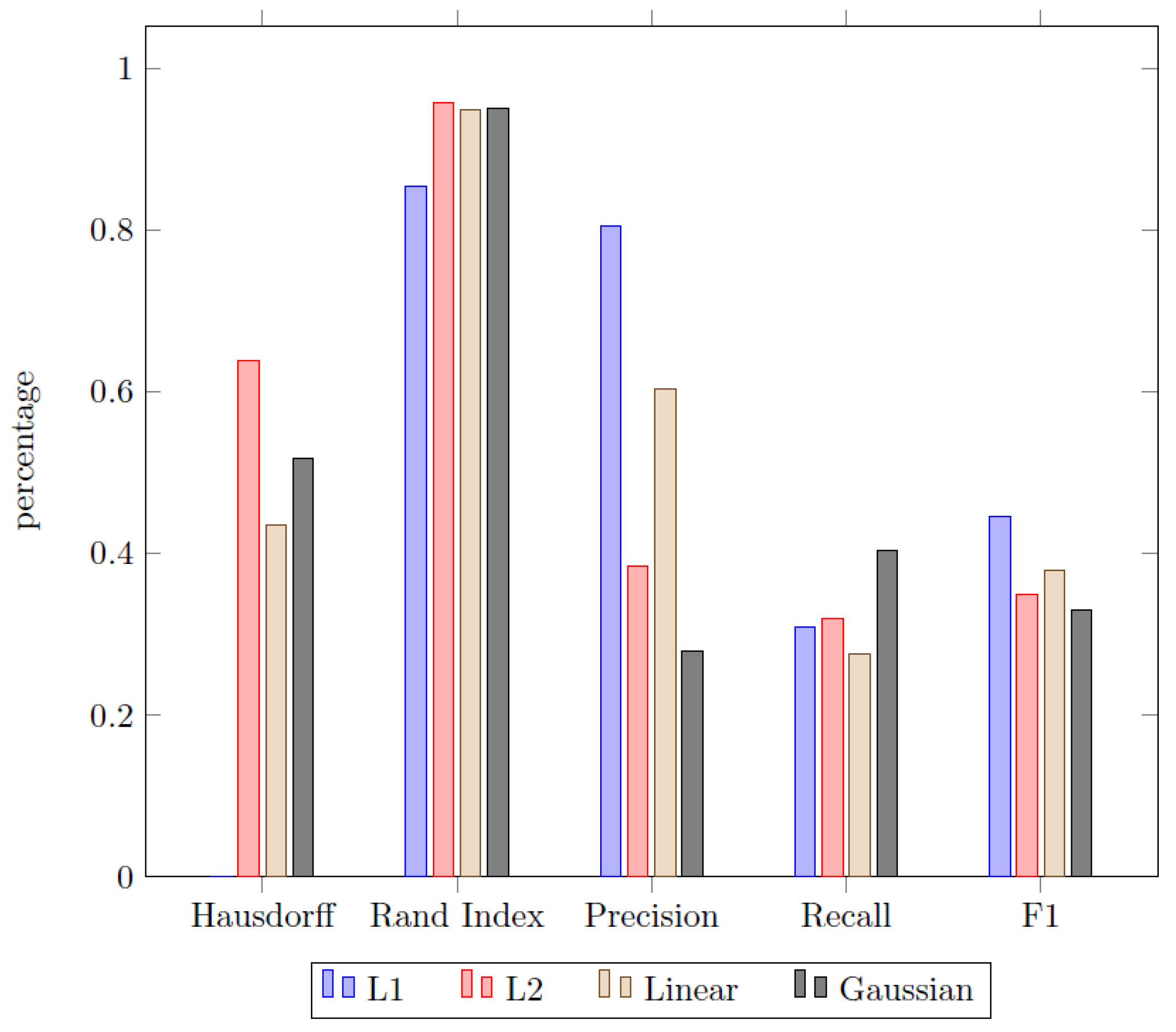
The first aspect of the experimental results deals with the problem of choosing a proper cost function in order to identify homogeneous segments. Therefore, a variety of different cost functions have been applied to the dataset by using the Sliding window approach discussed earlier. The results are displayed in
Figure 11.
Since both the Rand index and the F1-score are measures in the range , the Hausdorff metric is scaled accordingly. This is done by measuring the pairwise percentage difference of a given cost function in comparison to the worst result of the whole set of cost functions. Therefore, the approach with the worst Hausdorff metric always scores a zero, while the other scores display the percentage superiority of each approach in comparison to that. For the analytics problem used in this paper, we compared four different cost functions in total:
least absolute deviation (L1),
least squared deviation (L2),
linear model change based on a piecewise linear regression (Linear),
function to detect shifts in the means and scale of a Gaussian time series (Gaussian).
The findings displayed in
Figure 11 were found to show mixed results. While the L2 function scores superior in the field of temporal distance and recall, it is inferior in regard of the precision and ultimately in the total F1-Score. The L1 cost function on the other hand scores poorly in terms of the Hausdorff metric (L2 is relatively more than 60% better) but dominates the other approach in terms of precision and consequently scores best in term of the F1-Score. The two remaining cost functions remain unremarkable, since they consistently score significantly worse than the leasing approach for each metric category, except for the recall since all of the approaches are close there. In the end, the classical L2 cost function was chosen as benchmark for the comparison of the pathway methods based on its superiority in two out of three measures (Hausdorff and Rand index). This was also used in the following analysis and discussion of the results.
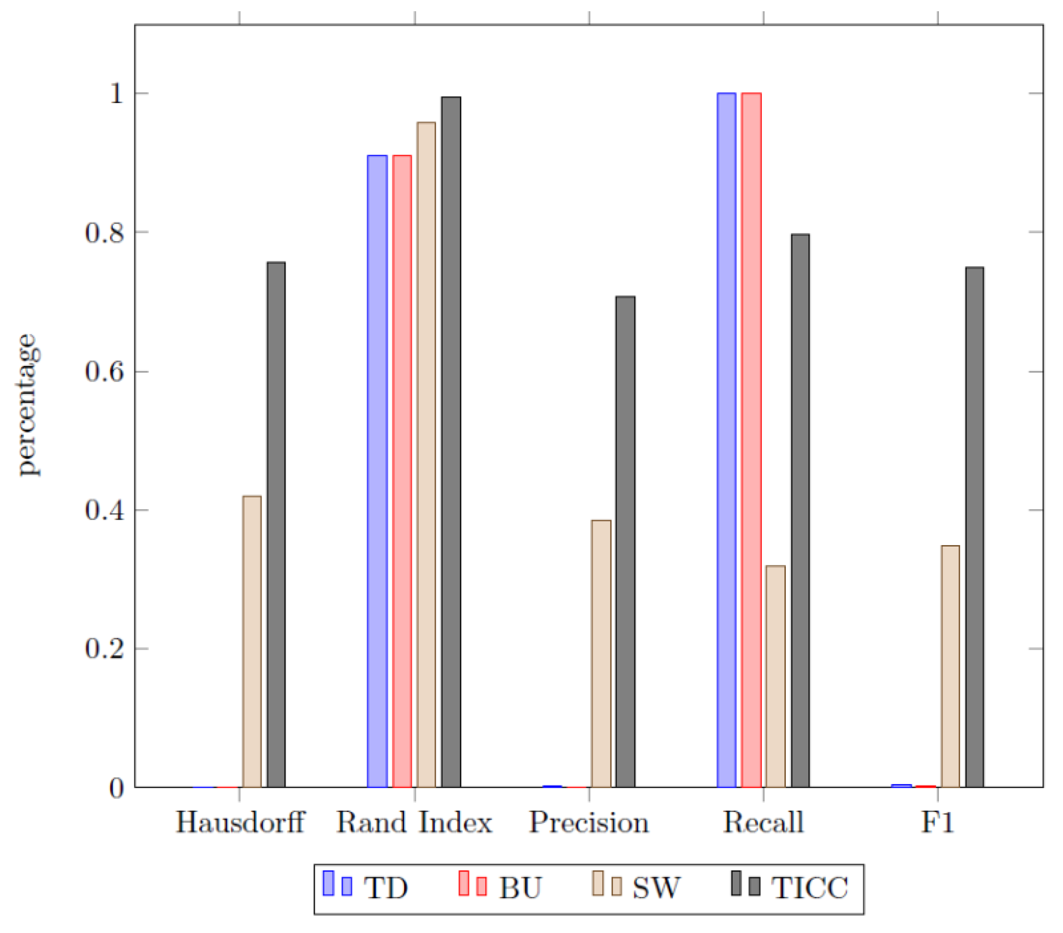
The second area of investigation is the comparison of the different searching methods with each other. The TICC algorithm was also included into this comparison by dropping the cluster labels from the results and therefore turning the multi-cluster output into a binary clustering (“steady mode” and “event”). The results are presented in
Figure 12.
The most striking result of the experiment is the superiority of the TICC approach in comparison to all heuristic methods. Even the best historical approach, namely sliding window, which has constantly outperformed the other two approaches except for the recall, is surpassed by the TICC algorithm remarkably.
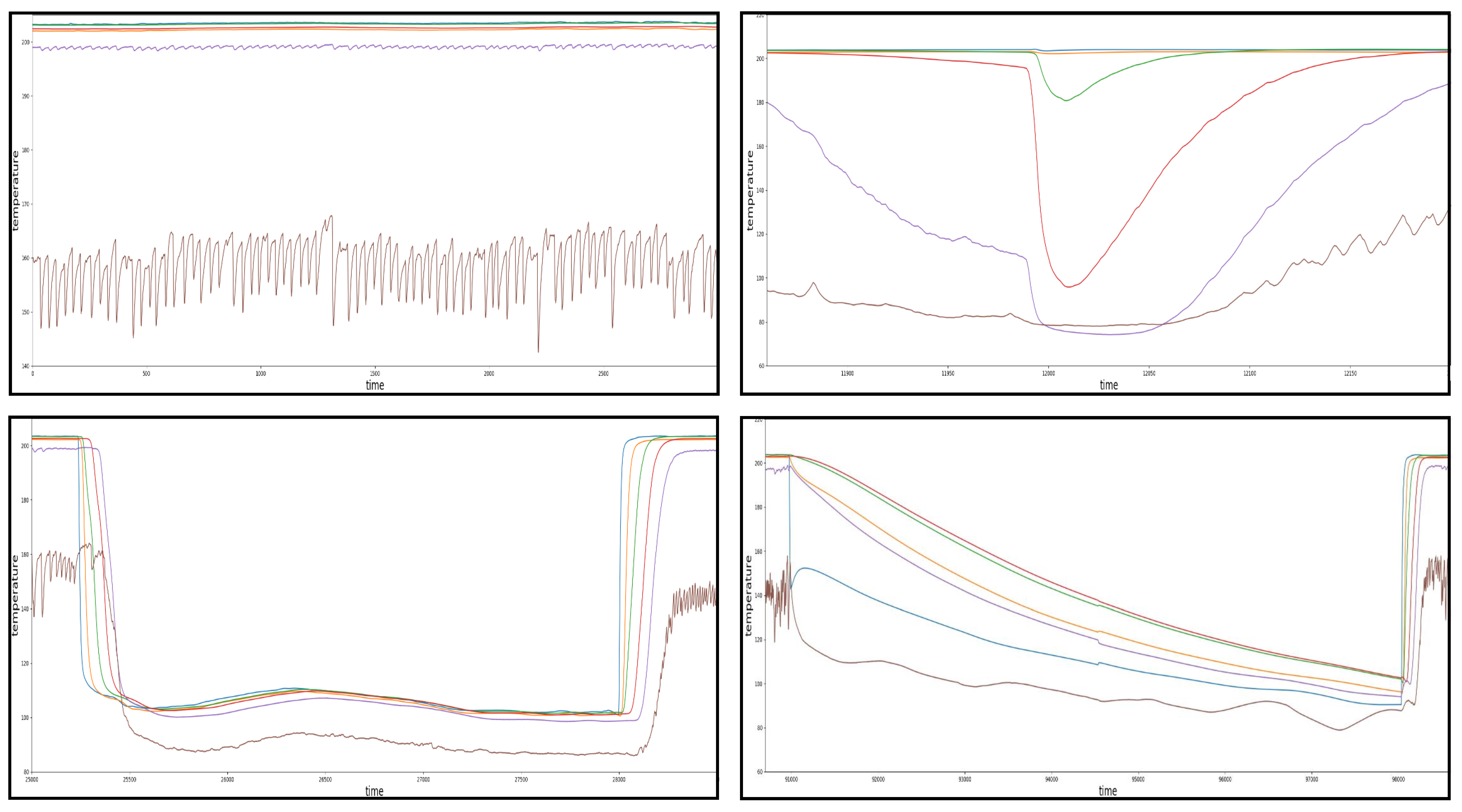
The pattern recognition approach provided by TICC identified a total of 32 events (disturbances of steady state), which in turn were broken down into four different clusters (patterns). Furthermore, it revealed the existence of not one but two steady states of the machine, which could not be identified by solely monitoring the temperature zones. The remaining three clusters were identified as actual disturbances of the drying process. An overview over all major events is given in the following
Figure 13. The pattern in the top left of the diagram represents a section of the steady state (cluster A) of the machine and depicts the natural fluctuations, especially of the sixth temperature zone (material input).
The first disturbance of this natural state can be seen in the bottom left of the diagram and will be referred to as cluster C or “canyon”. The disturbance occurred in total 10 times during the whole monitoring period with a mean duration of about 3000 min, which corresponds to approximately 46 h from start to the finish. The shortest duration of a cluster C events was 1530 min (25.5 h) and the longest duration was 3210 min (53.5 h).
The second recorded disturbance can be seen in the bottom right and is referred to as cluster D or “shark fin”. It appeared in total six times and was more fluctuant in terms of its durations, varying from approximately 1500 min (25 h) to 7300 min (121 h). The duration with the highest density (3 of 6) was thereby 1500 min (median).
The last common disturbance can be seen in the top right of the diagram and is referred to as cluster B or “random spike”. This disturbance appears less systematic then the events presented before since its durations range from 50 min to 400 min, which is notably shorter than the other common disturbance durations identified. The shape of the events of cluster B, which appeared a total of nine times, also can be seen to be less homogeneous in comparison to cluster C and D.
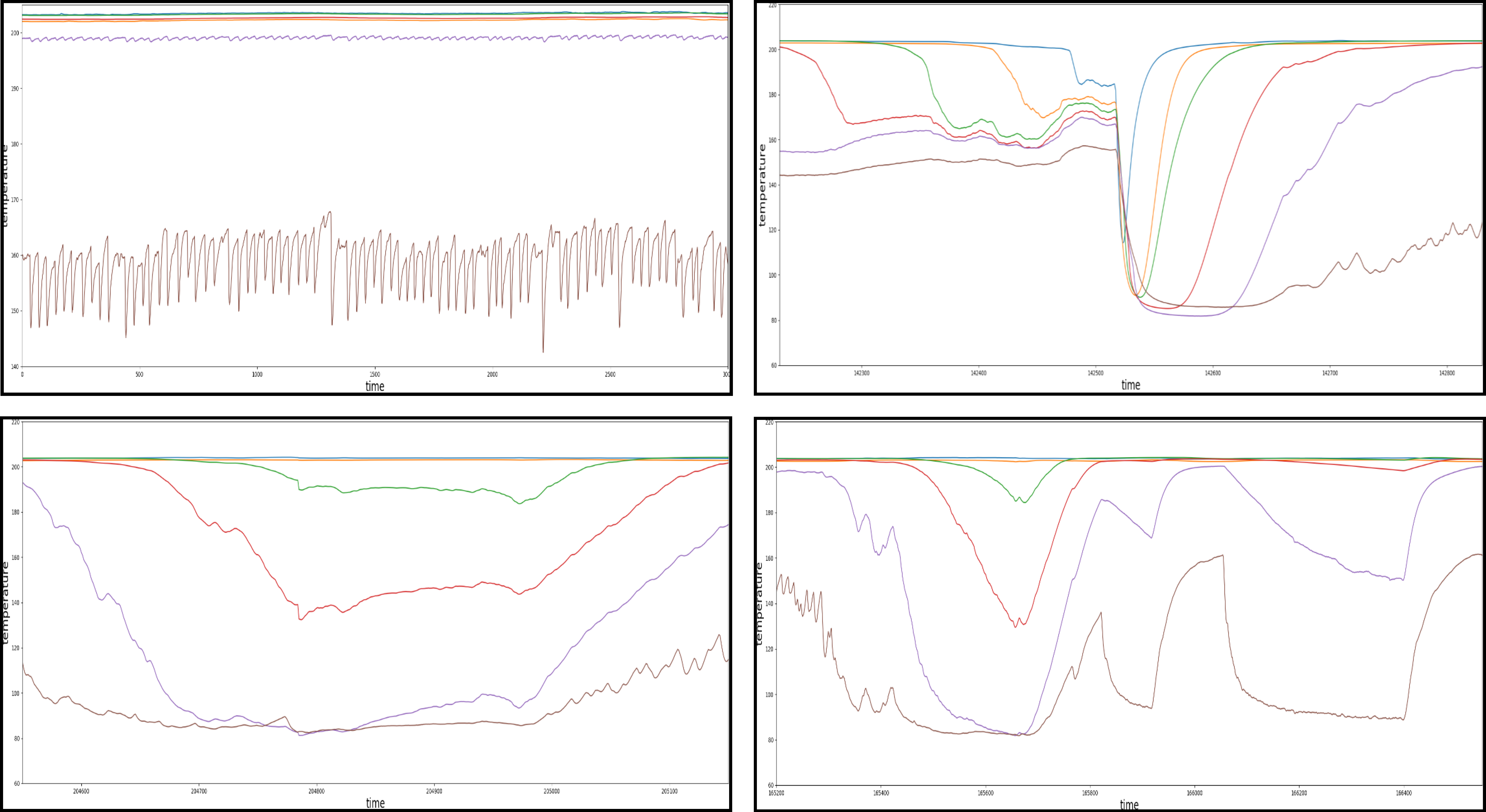
However, in addition to correct assignments the algorithm has made automatically, there have been some events which raised doubt in terms of their affiliation to the assigned failure clusters. Those irregularities are presented in the following
Figure 14.
The top left of the diagram shows the steady state as a comparison. The other three events show a characteristic pattern respectively but were still all assigned to the cluster C (“canyon”). However, in a later step of the manual analyzing process they have been found to be significantly different from the corresponding evens in the cluster C, therefore declared as related subclusters. Each of the subclusters occurred a total of two times within the entire dataset.
5. Discussion
This paper presents a functional framework to automatically analyze multivariate times series data in order to identify reoccurring patterns within a manufacturing setting. In doing so, we have tested two different pathways to approach the pattern recognition problem in time series applications and thereby displayed their strengths and weaknesses. As the data sets and their requirements vary significantly even within the manufacturing domain, the option to quickly apply and evaluate different approaches is a key feature towards a robust framework. However, to truly reflect the full wealth of different data sets and time series, additional alternatives might have to be included in the future. Nevertheless, the process and evaluation enable the principle scalability of the presented framework.
We have shown that a two-step approach of using a segmentation before clustering the data appears to be inferior to a collaborative method. The obtained results from our manufacturing time series data set have shown that even the first step of the sequential approach (heuristic segmentation) has already returned a worse performance for all possible searching methods when compared to the TICC approach in this case. This can be observed in the
Figure 12 of the results, since the TICC algorithm scored significantly higher in almost all statistical evaluation metrics. The only indictor where TICC scored below the alternative BU and TD approaches was the recall metric. This can, however, be easily explained in this context due to the low precision scores of both heuristic methods, since they have a tendency to oversegment the data. A rather fine partitioning consequently increases the probability that the true change points will be among the predicted set, but consequently increase the number of false (unnecessary) break points, reducing the precision drastically. The better performance of the TICC approach could also not be explained through an unproper cost function, since we have vetted various homogeneity metrics in order to identify the most suiting failure function for the given dataset (see
Figure 11). All in all, the finding indicates that the second processing pathway is the superior approach in this application case.
We have also shown that the TICC featuring pathway is capable of returning strong results, since all of the three major events in the times series have been found and furthermore assigned to different clusters. Even though it was not able to recognize the events displayed in
Figure 14, this can be explained though the low frequency of those disturbances and therefore a lack of significance in order to define a new cluster based on only a few available examples.
A further dissection of the cluster C and D suggests that those clusters correspond to the real-world activity of shutting the machine down for the weekend. National holidays were also taken into consideration and made it possible to explain a significant number of events that took part over the cause of a day or two. Furthermore, the differences in the cluster C and D might be the result of the difference between a rapid machine shutdown, were the material is removed immediately and a cooling process, were the material remained in the machine. This could also indicate an unproper shutdown, were the material was supposed to be removed for the weekend break but forgotten inside the dryer. The events assigned to cluster B (random spikes) could, however, not be tied to related real-world events at this point and most likely correspond to random disturbances caused for example by an improper handling of the machine or related short-term issues. However, the insights from the analysis can now be used to investigate the root cause and then return with a correct label for these events in the future after further consultation with domain experts. Like most analytics projects, the continuous cycle is key for a long-term sustainable solution and providing real value to the application area.
All in all, our results show that the multivariate clustering approach displayed in the second pathway is able to return strong results for the time series data set in this case. It is safe to say that the new framework can identify common events, which in some cases correspond with relevant sources of failure. Therefore, these insights can subsequently be used to implement a near real-time warning system (or as input for a more sophisticated predictive maintenance system) that is capable of not only identifying and correctly clustering disturbances, but also tying it to a real-world activity.
6. Conclusions and Future Work
This paper presents a framework to utilize multivariate time series data to automatically identify reoccurring failure patterns in a real-world smart manufacturing system. To do so, the mixed binary (on/off) and continuous (temperature) data provided by the monitoring system of an industrial drying hopper was analyzed following two different processing pathways. The first approach was built-up using a subsequent segmentation and clustering approach, the second branch featured a collaborative method at its core (TICC). Both pathways have been facilitated by a standard PCA analysis (feature fusion) and a hyperparameter optimization (TPE) approach.
The second procedure featuring TICC returned constantly superior results in comparison to all heuristic segmentation methods for the available time series data set. It was therefore expanded and finally enabled the recognition of three major (most frequent) failure patterns in the time series (“canyon”, “shark fin”, and “random spike”). Furthermore, it was also able to recognize all disruptions of the steady state but failed to identify all of the less frequent failure patterns as stand-alone clusters. Besides evaluating the statistical accuracy, we furthermore leveraged domain expertise to verify the results and were, e.g., able to identify one event (canyon) as a shutdown process that aligns with weekends and holidays.
Nevertheless, the identified cluster can be used subsequently to enhance the monitoring process of the drying machine even further and to establish a predictive maintenance system in order to foresee potential upcoming machine downtimes. This framework can also be applied to other (related) problems in the field of preventive maintenance and pattern recognition in time series in general. Industrial monitoring and maintenance systems can therefore be extended by adding a failure detection component to enhance the machine restoration process (speed) further. Such algorithms can also be used to automatically analyze large amounts of data generated by the machinery pool, thereby reducing the manual workload necessary for this process.
The presented framework can contribute to reducing unnecessary machine downtimes in the future, improve the troubleshooting process in case a failure occurs, and consequently increase the effective machine running time and overall productivity of the plant. An additional advantage from a managerial point of view is the possibility to automate the process and improved transparency of the production process.
However, there also ethical implications that need to be considered aside of the overall impact of the presented research findings on the business process and workflow. On the one hand, the increase in efficiency is not only favorable for the business objectives overall due to the potential cost reduction, but also to the society in general given potential improvement of environmental (e.g., reduction in co2-emissions and overall waste of energy) and working atmosphere (e.g., reduction of unnecessary stress from unplanned machine failure) benefits. On the other hand, those techniques may also present an opportunity for being abused when other types of time-series data, such as personal data, of workers, are analyzed. For instance, biometric and behavioral data can be monitored and analyzed automatically, potentially leading to issues with regard to privacy and other negative implications for workers. Thus, it is necessary to investigate policy implications hindering inappropriate application of such time-series analytics conflicting with individuals’ privacy rights.
The presented process and analytical model are influenced by design and thus to a certain extend limited. Since the whole performance measuring process (correct number of clusters) is dependent on the manual determination of the true change points and clusters (or subclusters) it reflects a certain subjectivity and dependence on domain knowledge and metadata. Furthermore, the overall clustering approach is initialized through a distance-based algorithm (k-means), which makes it biased in terms of its priors and the subsequent estimation of the Gaussian mixture distributions. The effectiveness of the proposed framework can also not be guaranteed for the entirety of industrial domains since it was only tested on one specific dataset from a particular field. In order to address these challenges, future research should focus on follow up studies to improve the framework in respect to the algorithmic initialization and study the applicability of the underlying concept on similar use-cases in the industrial domain. Additionally, comparing the methodology to other approaches in further studies using a comparable data set will increase the transparency and understanding of its value.


