
Statistical Analysis of Mesoscale Eddies Entering the Continental Shelf of the Northern South China Sea


1
Laboratory of Coastal Ocean Variation and Disaster Prediction, Guangdong Ocean University, Zhanjiang 524088, China
2
Fourth Institute of Oceanography, Ministry of Natural Resources, Beihai 536000, China
3
Key Laboratory of Continents-Deep Sea Climate, Sources and Environments, Zhanjiang 524088, China
4
Key Laboratory of Space Ocean Remote Sensing and Application, MNR, Beijing 100081, China
5
Department of Atmospheric and Oceanic Science, University of Maryland, College Park, MD 20742, USA
*
Author to whom correspondence should be addressed.
J. Mar. Sci. Eng. 2022, 10(2), 206; https://doi.org/10.3390/jmse10020206
Submission received: 28 December 2021
/
Revised: 25 January 2022
/
Accepted: 26 January 2022
/
Published: 2 February 2022
(This article belongs to the Special Issue Frontiers in Physical Oceanography)
Abstract
:An Archiving, Validation and Interpretation of Satellite Oceanographic data (AVISO) mesoscale eddy trajectory atlas product is used to analyze the path type and temporal variability of the eddies that entered the continental shelf area of the northern South China Sea (SCS) from 1993 to 2016. A total of 184 mesoscale eddies entered the continental shelf area of the northern SCS during a 24-year period. We classify the mesoscale eddies into four types according to the motion trajectories: along-the-isobath type, intrusion-of-continental-shelf type, local wandering type, and shelf-internal-generation type. The occurrence numbers of these four types were 87, 38, 23, and 36, respectively. The mean amplitude and radius of the along-the-isobath type are the largest, about 18 cm and 153 km, respectively; furthermore, their average lifetime is also the longest, about 93 days. The mean amplitude, radius, and lifetime are the smallest for the shelf-internal-generation type, about 16 cm, 146 km, and 74 days, respectively. The direction and velocity of the background flow field affects the intrusion path of the mesoscale eddies onto the continental shelf of the northern SCS. The seasonal distribution of the mesoscale eddies quantity is also related to the direction and velocity of the corresponding background flow field.
1. Introduction
Ocean mesoscale eddies (also called oceanic vortices) are long-term close-circulation regions within the ocean [1,2,3]. Their spatial scales measure between tens and hundreds of kilometers, and the temporal scales measure between tens and hundreds of days [4,5]. In a vertical direction, their scales range from a few tens-of-meters to the whole ocean depth [2].
Mesoscale eddies exist widely throughout the global ocean [6,7], and their energy is higher than the background flow field for an order of magnitude [8]. They can be induced by the instability of ocean currents, a geostrophic adjustment after convection, or via topographic influences [1,2]. The mesoscale eddies account for approximately 90% of the total kinetic energy of the ocean circulation [9]. They are considered to be one of the most important dynamical processes in the upper ocean [10] as they play an important role in marine matter, momentum fields, heat transport, and circulation structure, as well as affecting chemical exchange processes and marine ecosystems.
The development of the satellite altimeter has promoted the tracking and statistical study of mesoscale eddies. Chelton et al. [7] used 10 years of satellite altimeter data to calculate the basic characteristics of global mesoscale eddies. In the longitudinal direction, more than 75% of mesoscale eddies propagate westward, and the westward velocity decreases with latitude. In the latitudinal direction, cyclonic and anticyclonic mesoscale eddies propagate poleward and equatorward, respectively. Eddies with radii of 50–150 km account for more than 90% of the total number of global eddies.
The SCS is located in the region 2.5–23.5° N and 99.2–121.8° E. Its eastern side is connected to the Northwest Pacific Ocean via the Luzon Strait. The western area extends to mainland Southeast Asia. The SCS is the largest semi-enclosed marginal sea in the northwest Pacific Ocean. The depth varies between 200 and 6000 m [11]. The average depth is approximately 2400 m [12]. The total area is approximately 3.5 × 10⁶ km2, of which approximately 48% is shallow sea, defined as a depth less than 200 m. During the summer, southwesterly winds prevail in the SCS; while, during the winter the dominant wind direction is reversed due to the interaction between the topography and the northeasterly monsoon. The SCS also shows different circulation patterns during the summer and the winter. At the same time, the outer eastern side of the Luzon Strait is affected by the Kuroshio. The geographical location, the monsoon effects, the circulation characteristics, and the complex dynamic background of the SCS lead to its unique marine environment.
The mesoscale eddies in the SCS have been studied by previous investigators [13,14,15,16,17,18]. Using temperature and salinity data, Wang et al. [19] observed an anticyclonic warm eddy located in the southwestern part of Taiwan Island. They considered that the eddy originated from the Kuroshio intrusion. Through multiple navigation observations Wang et al. [20] determined that there is a perennial warm eddy near Luzon Island. Xiu et al. [21] counted the number of mesoscale eddies in the SCS between 1993 and 2007 using sea surface height anomaly data. They found that the annual average number of mesoscale eddies generated in the SCS is approximately 32.9 ± 2.4, and about 52% of them are cyclonic eddies. Wang et al. [22] used the global Simple Ocean Data Assimilation (SODA) analysis system dataset from 1958 to 2007 to obtain an average of 28.4 eddies generated annually in the SCS.
The northern shelf of the SCS is a broad shelf that orients from the northeast to the southwest. The flow system of the northern shelf of the SCS is complex and consists of: the southwestward slope current, the SCS warm current between the slope and the shelf, the coastal currents with opposite directions in winter and summer, and winter downwelling [23]. Under the control of the monsoon and the general circulation, complex and variable ocean dynamic processes occur in the northern shelf area of the SCS; understanding these is essential to the study of the dynamic marine environment of the SCS.
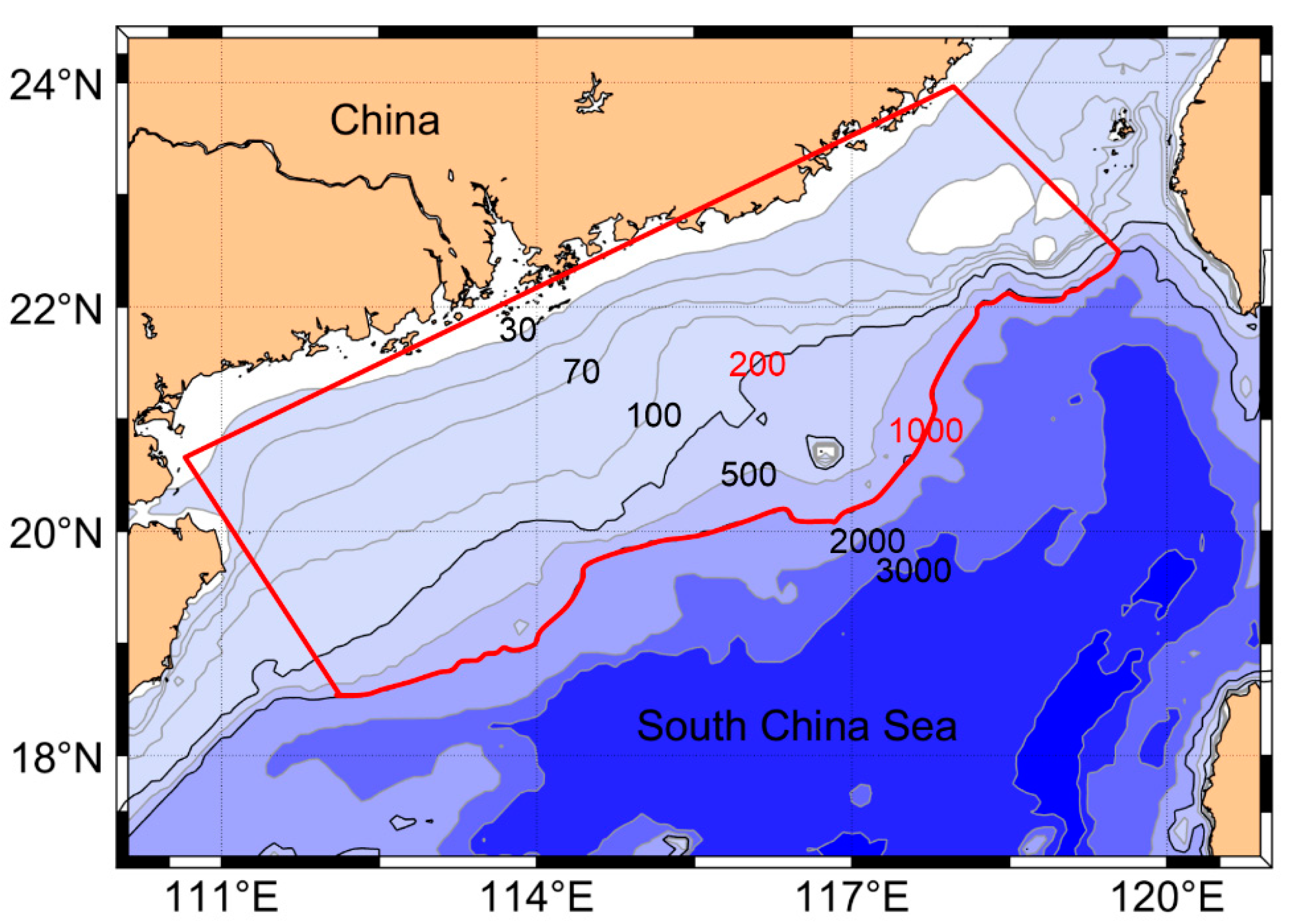
Previous studies on ocean mesoscale eddies have mostly focused on the mesoscale eddies in the deep basin of the SCS; however, one-third of mesoscale eddies would reach areas where the depth is less than 1000 m in the ocean [7]. The continental shelf in the northern SCS is broad, about 200 km wide. What happened to the mesoscale eddies that reached this wide continental shelf area? This study focuses on mesoscale eddies that entered the continental shelf area of the northern SCS (as shown in Figure 1). The temporal distribution of the mesoscale eddies is analyzed, as well as their paths.
2. Data and Methods
2.1. Eddy Tracking Data Set
The mesoscale eddy trajectory atlas product is derived from the two-satellite daily delayed time gridded sea level anomalies product, originally distributed by AVISO (https://www.aviso.altimetry.fr/es/data/products/value-added-products/global-mesoscale-eddy-trajectory-product.html (accessed on 27 January 2022)), with 0.25° in spatial resolution. It is processed using algorithms derived from Chelton et al. [7]. The eddies are identified as features with diameters of 100–300 km, and a filter is applied to remove short tracks (less than 28 days). The data set includes information such as mesoscale eddy amplitude (defined as the maximum sea level anomaly), rotational speed, radius, position, and observation time. The data are collected from 1993 to 2016 with a temporal resolution of 1 d.
2.2. Flow and Vorticity Field Data
The daily mean total surface and 15 m current velocities data product used here is obtained from the Copernicus Marine Environment Monitoring Service (CMEMS), (http://marine.copernicus.eu/services-portfolio/access-to-products/?option=com_csw&view=details&product_id=MULTIOBS_GLO_PHY_REP_015_004 (accessed on 27 January 2022)). The data set contains fields with a spatial resolution of 0.25° × 0.25° from 1993 to 2016.
The daily mean vorticity field is calculated from the daily mean total surface and 15 m current velocities data product as , where u and v are the zonal and meridional components of the current velocity; x and y are the geographic distance for spatial resolution in the zonal and meridional direction, respectively.
3. Results
According to the data set, there were 184 mesoscale eddies that entered the study area during the period from 1993 to 2016. The number of anticyclones was 96, which accounted for 52.2% of the total number of vortices. The number of cyclones was 88, which accounted for 47.8%. The number of anticyclonic eddies was more than the number of cyclonic eddies.
3.1. Interannual Characteristics of the Mesoscale Eddies
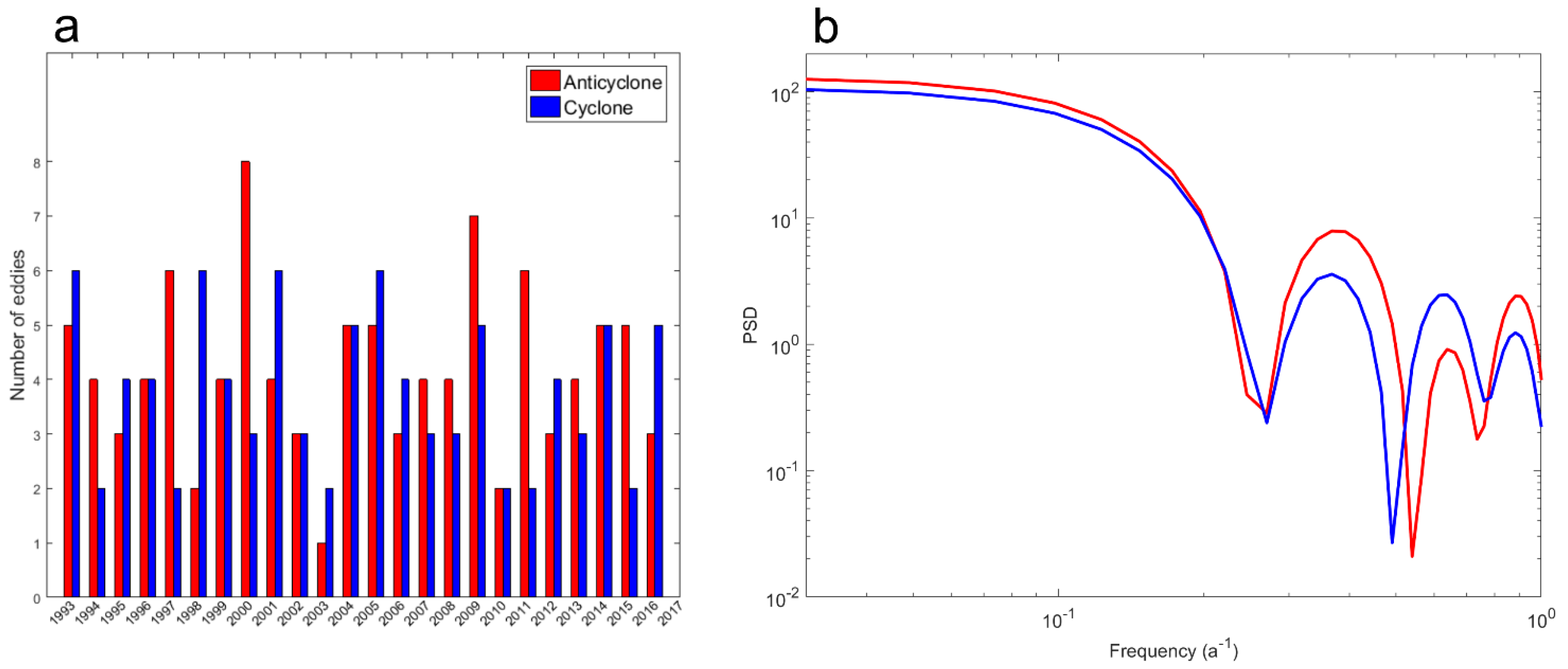
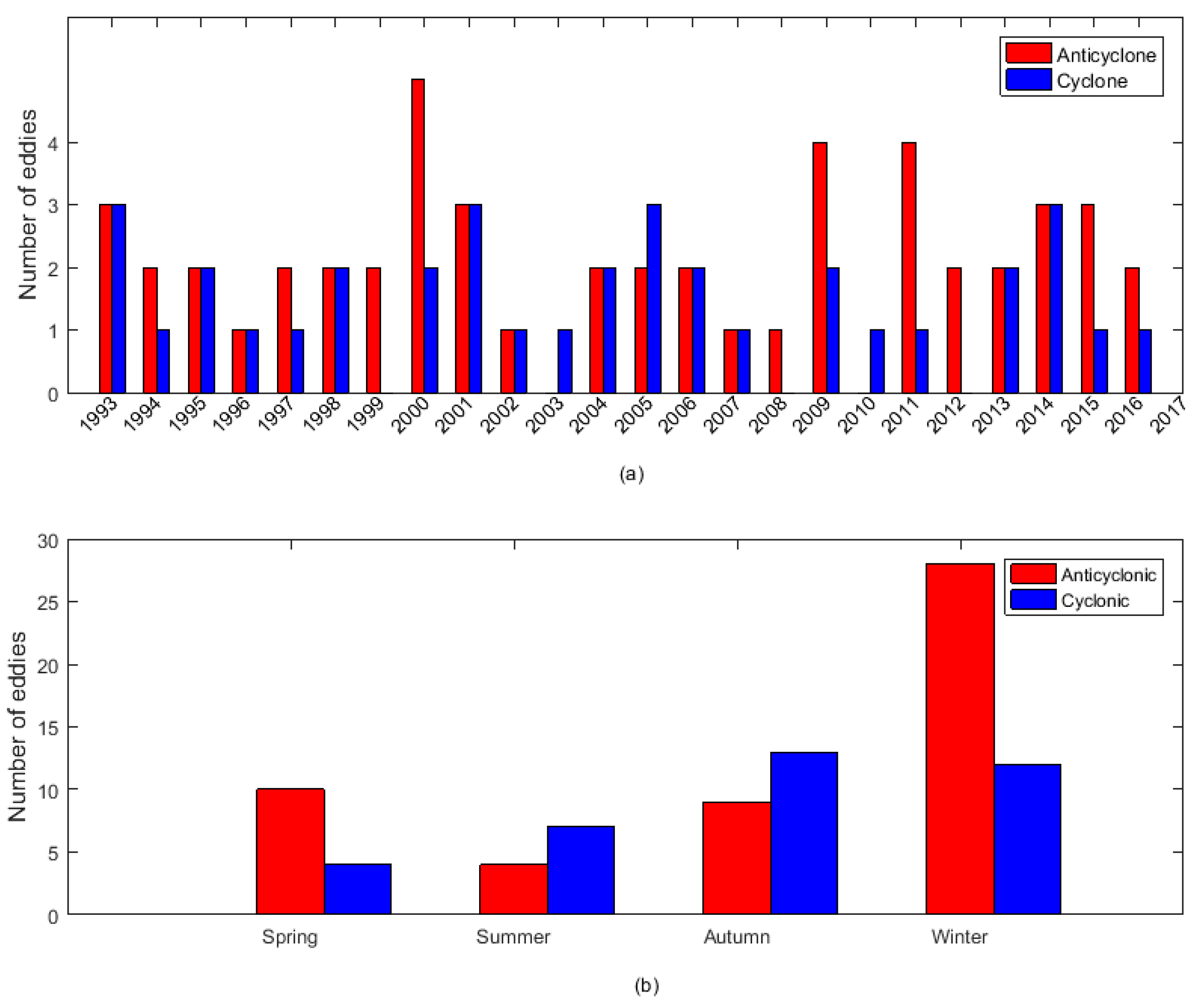
The temporal distribution of the number of eddies, as shown in Figure 2, indicates significant interannual variations. One can see the following features: (1) The mean number of the mesoscale eddies is about eight, which means that one eddy would intrude into the study area every 1.5 months, (2) the spectra for temporal distribution of the number of eddies peaked at periods of 2–3 years, which shows a significant inter-annual variation, (3) the number of cyclonic eddies that invaded the study area in 1994, 1997, 2003, 2010, 2011, and 2015 is two, which is less than the average, (4) there is an excessive number of anticyclonic eddies in 1997, 2000, 2009, and 2011. Furthermore, the major El Nino events occurred during 1994, 1997, 2003, 2010, and 2015; therefore, an El Nino event should lead to fewer cyclonic eddies in the study area.
3.2. Seasonal Characteristics of Mesoscale Eddies
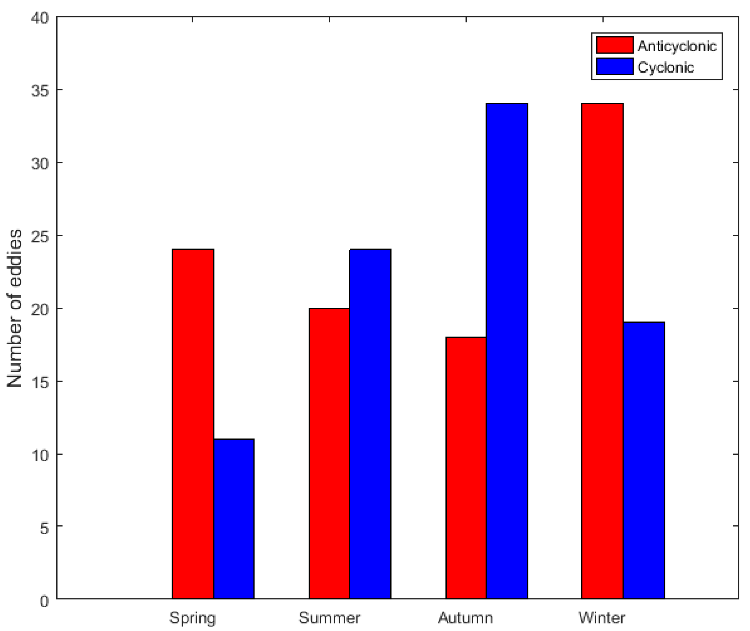
The seasonal average number of mesoscale eddies entering the study area from 1993 to 2016 is shown in Figure 3. As we can see, the number of cyclonic mesoscale eddies during the summer and the autumn is significantly more than during the spring and the winter. However, the number of anticylonic eddies during the spring and the winter is more than twice the number of the summer and the autumn. The temporal distribution of the cyclonic eddies in the study area is opposite to that of the anticylonic eddies. The total number of eddies during the autumn and the winter is more than during the spring and the summer.
The total number of eddies during the autumn and the winter is more than during the spring and the summer, therefore it seems that this is related to the wind stress in the area. Cheng et al. [24] calculated the seasonal wind stress of the SCS from 2000 to 2003 using QuikSCAT wind field data. The results show that the strong cyclonic wind stress rotation is distributed during the autumn and the winter. Li et al. [25] analyzed the root-mean-square (RMS) values of the sea surface height anomaly during 1993–1999, and concluded that there is clear seasonal behavior in the northeastern SCS, with high RMS values of the sea surface height anomaly mainly occurring from July to February, and low values from June to March.
Southwesterly winds prevail during the summer, and the dominant wind direction is reversed during the winter; moreover, the seasonal distribution of cyclonic and anticyclonic eddies indicates an inverse phase. As the upper ocean circulation is mainly driven by wind stress, the positive wind-stress curl results in a cyclonic circulation in the SCS basin during the winter. The cyclonic circulation during the winter is accompanied by anticyclonic eddies.
3.3. Eddy Path Classification
We classify the mesoscale eddies during the period from 1993 to 2016 into four types according to their motion paths: (1) the along-the-isobath type, which moves along the isobaths after entering the study area, (2) the intrusion-of-continental-shelf type, which invades the continental shelf, (3) the local wandering type, which enters the study area and wanders the area for several weeks, (4) the shelf-internal-generation type, which is generated within the study area.
3.3.1. Along-the-Isobath Type
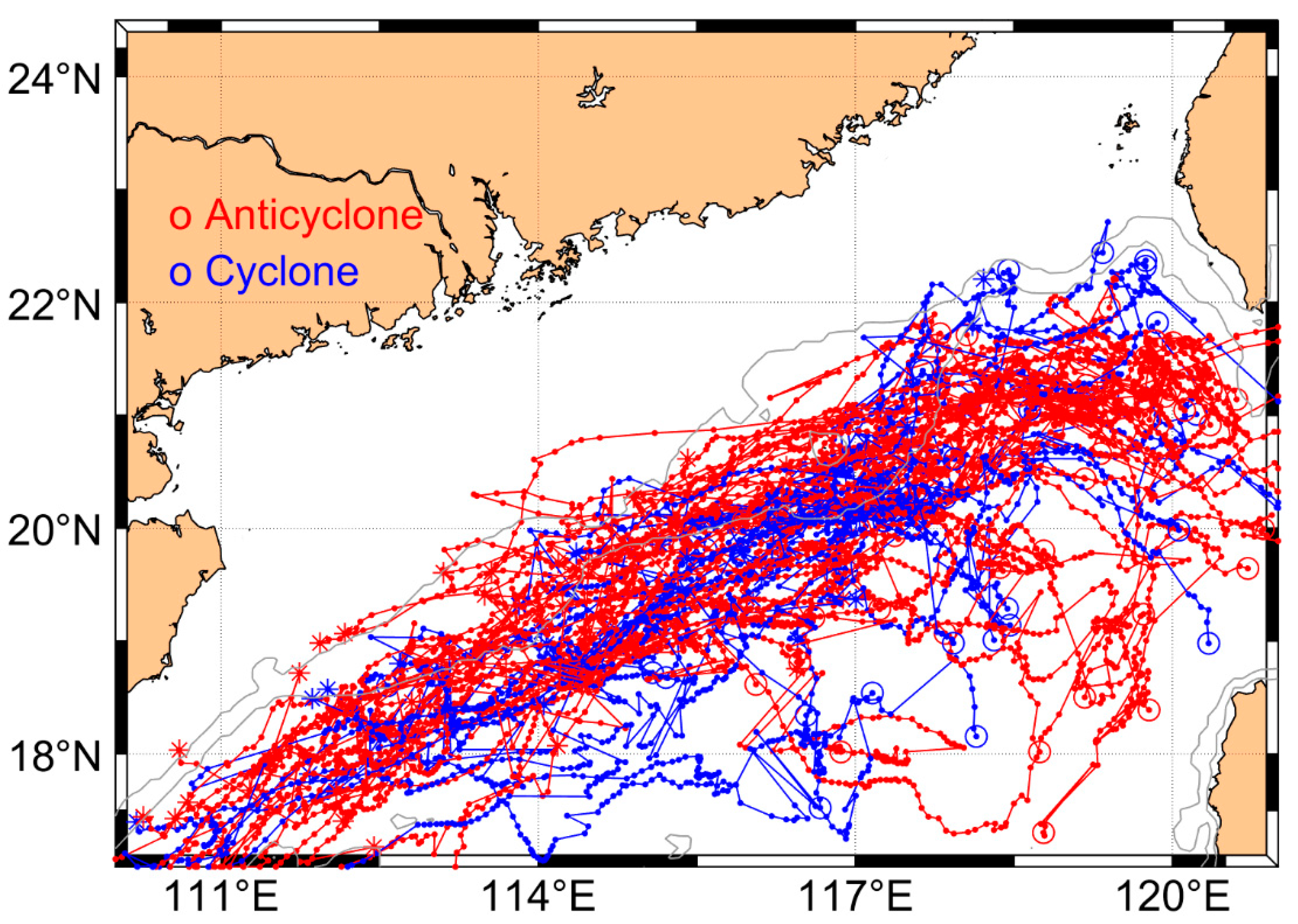
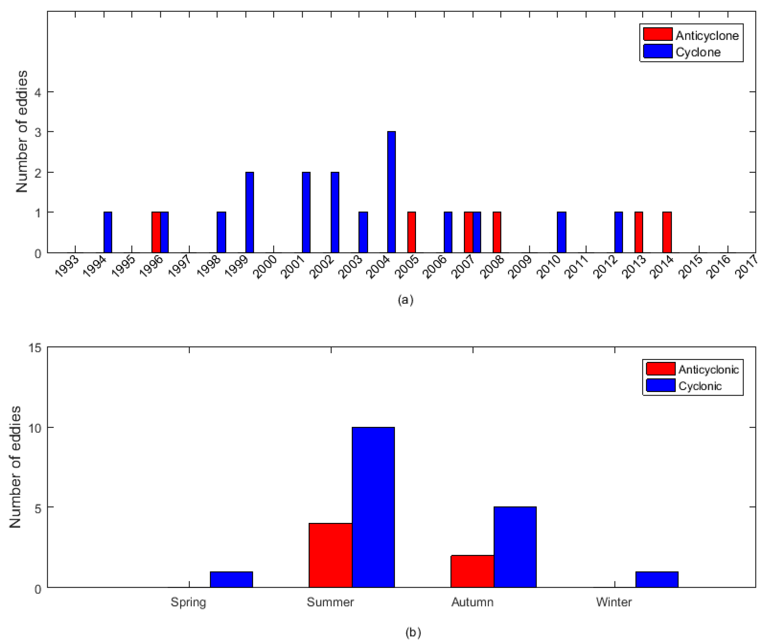
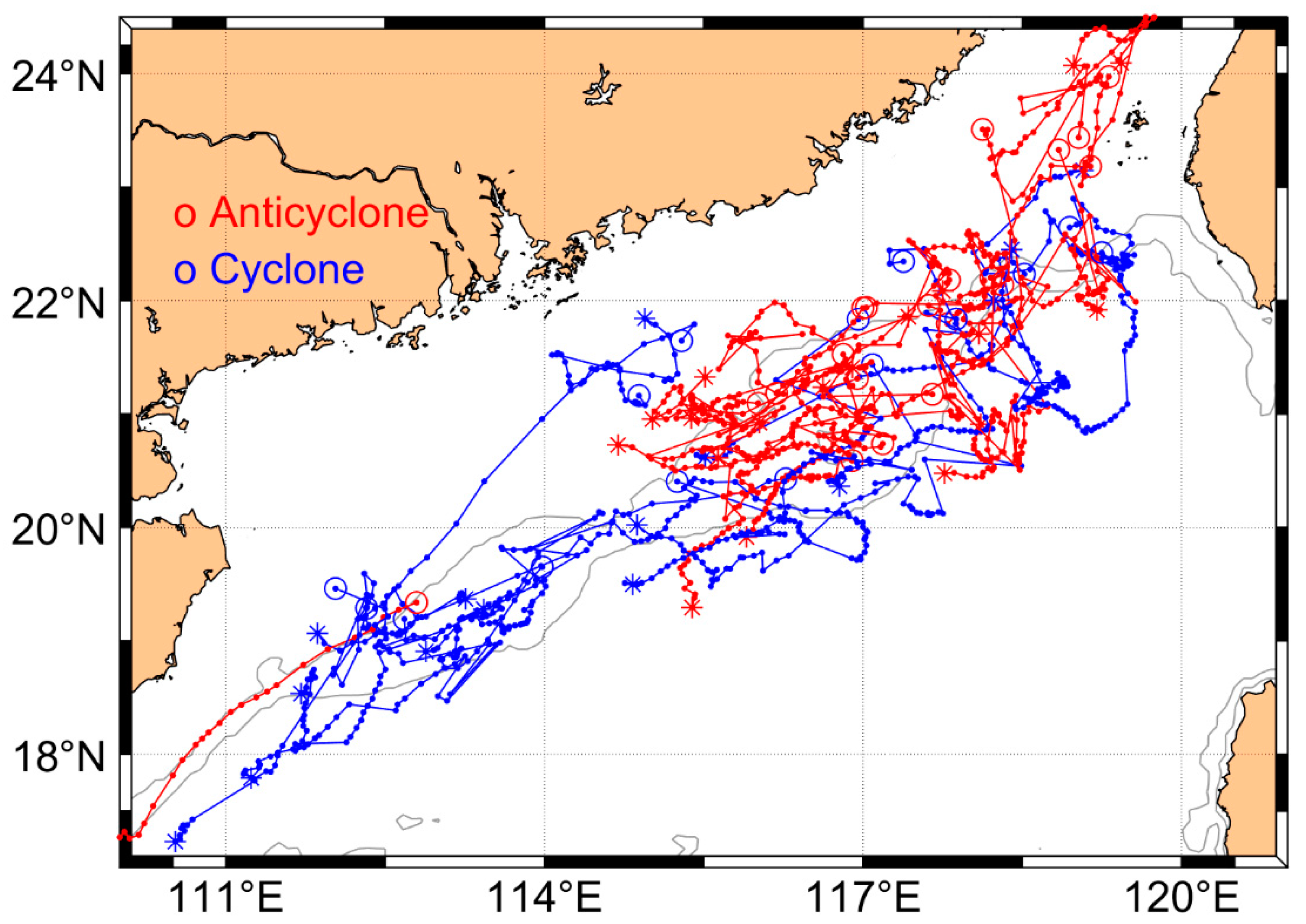
This type accounts for 47.3% (87) of the total mesoscale eddies during the 24-year period. The pathway of this type is shown in Figure 4. As we can see, these mesoscale eddies are generated in most cases in the northeast area of the SCS. After entering the study area, they move along the 1000 m isobaths, then arrive at the northwest area of the SCS. We analyzed the temporal variability of eddies of the along-the-isobath type, as shown in Figure 5. One can see that the number of anticyclonic eddies is more than the number of cyclonic eddies. The number of these eddies is smaller during 1994, 1996, 1997, 2002, 2003, 2007, 2008, and 2010. The number of these eddies reaches a peak during the winter (about 40 eddies), and the number of anticyclonic eddies is double the number of cyclonic eddies. The smallest number of eddies (11) is observed during the summer.
We calculated the mean lifetime, amplitude, and radius for the along-the-isobath type eddies, as shown in Table 1. The average survival time for this type of mesoscale eddy is 93 days (up to 328 days). The average amplitude is 18 cm. Additionally, the average radius is 154 km.
3.3.2. Intrusion-of-Continental-Shelf Type
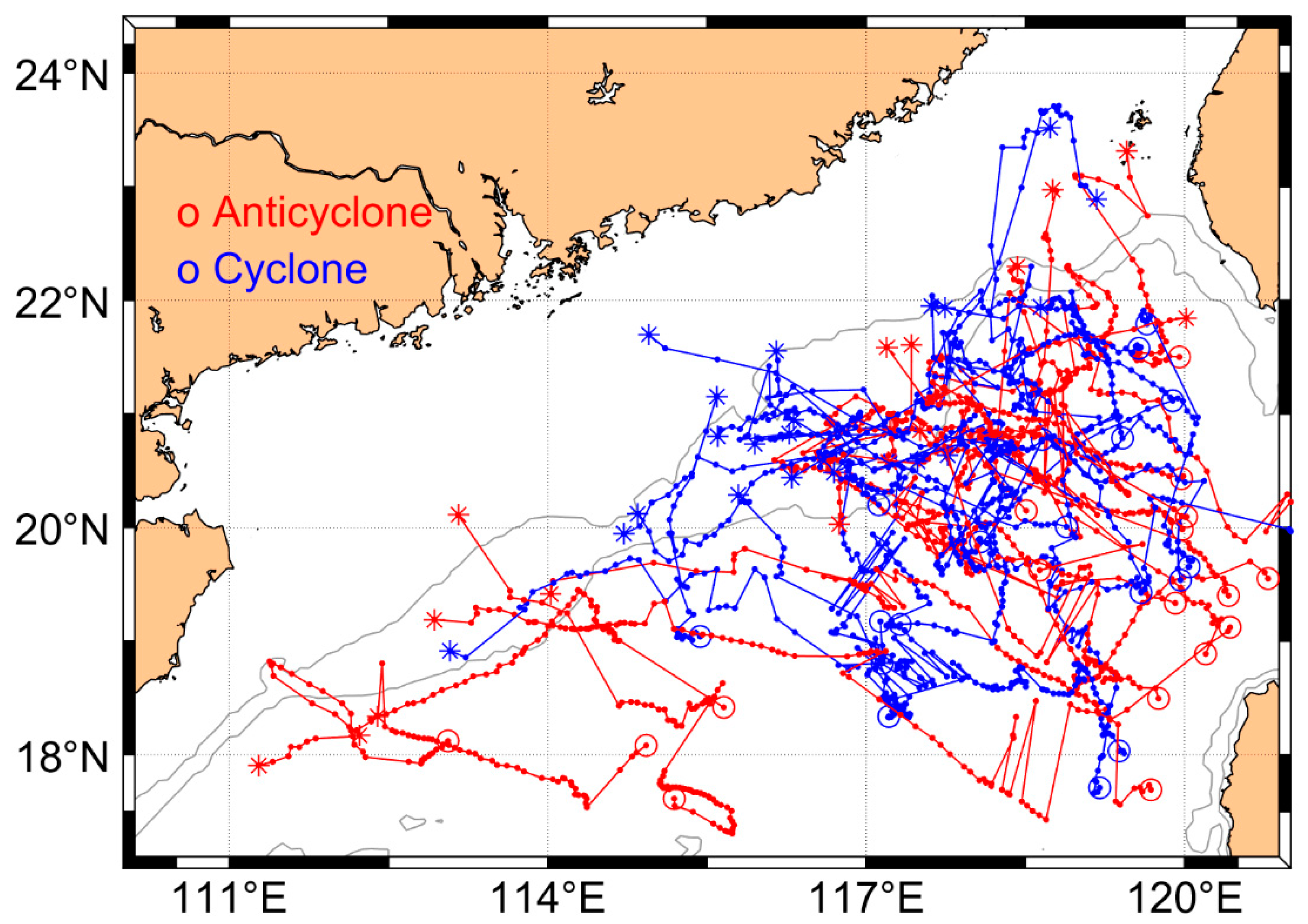
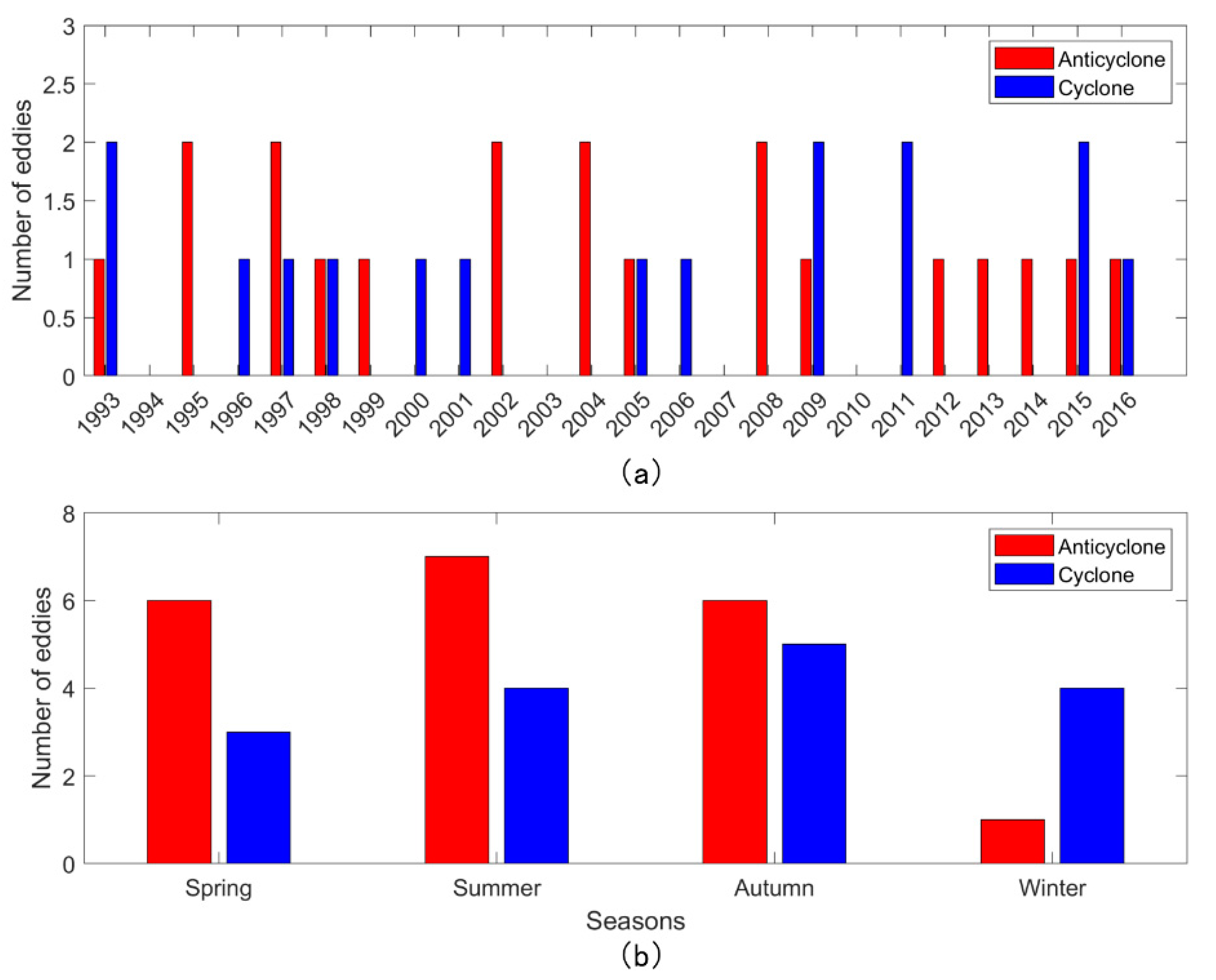
The intrusion-of-continental-shelf type of mesoscale eddies accounts for 20.7% (38) of the total samples from 1993 to 2016. The pathways are shown in Figure 6. One can see that the cyclonic eddies are concentrated on the east side of the study area (east of 116° E). The eddies seem to die quickly after they intrude the continental shelf. Only five eddies reached the area with a depth less than 200 m.
The temporal variability of the intrusion-of-continental-shelf type is shown in Figure 7. It can be seen that there is about one mesoscale eddy per year that invades the continental shelf of the northern SCS. Additionally, the anticyclonic eddies of this type are distributed in the western area of the study area (west of 116° E) for 1999, 2008, 2009, and 2010, all of which are strong La Niña years. The number of anticyclonic and cyclonic eddies are 17 and 20, respectively. One can also see that the number of eddies during the spring and the autumn is much more than during the summer and the winter, which indicates that the intrusion events occur during the spring and the autumn.
According to the statistics shown in Table 2 the average survival time of the intrusion-of-continental-shelf mesoscale eddies is 82 days, up to 213 days, the average amplitude is 17 cm, and the average radius is 149 km.
3.3.3. Local Wandering Type
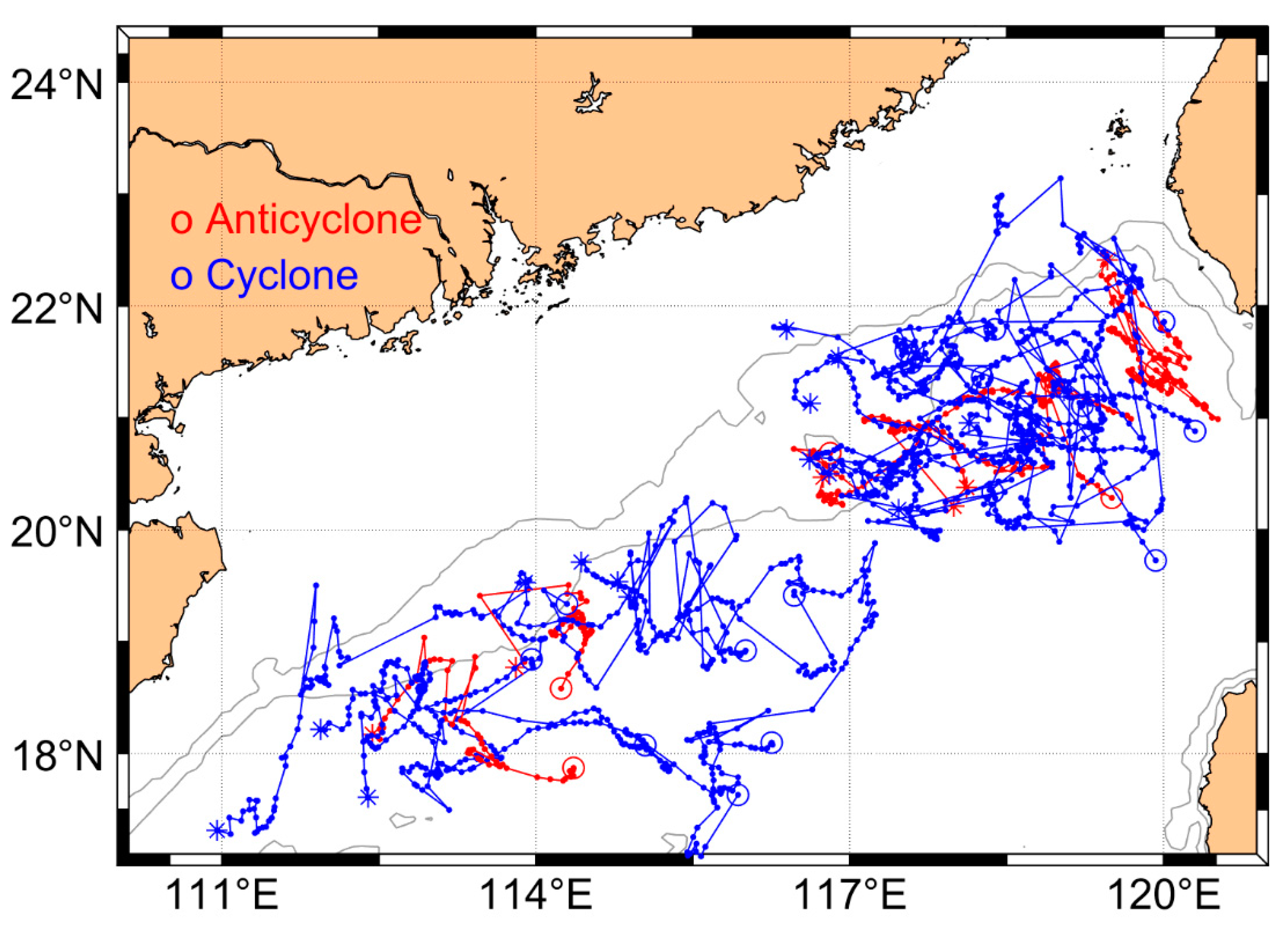
The local wandering type of mesoscale eddies accounts for 12.5% (23) of the total eddies in the study area from 1993 to 2016. The pathways are shown in Figure 8. One can see that this type indicates a clear spatial distribution. The cyclonic eddies are mainly distributed in the west of the study area during the years when no strong ENSO event occurred. The strong ENSO events occurred in 1996 (strong La Niña year), 2005 (strong El Niño year), 2007 (strong El Niño year), and 2008 (strong La Niña year). During these years, the anticyclonic eddies were distributed in the east of the study area.
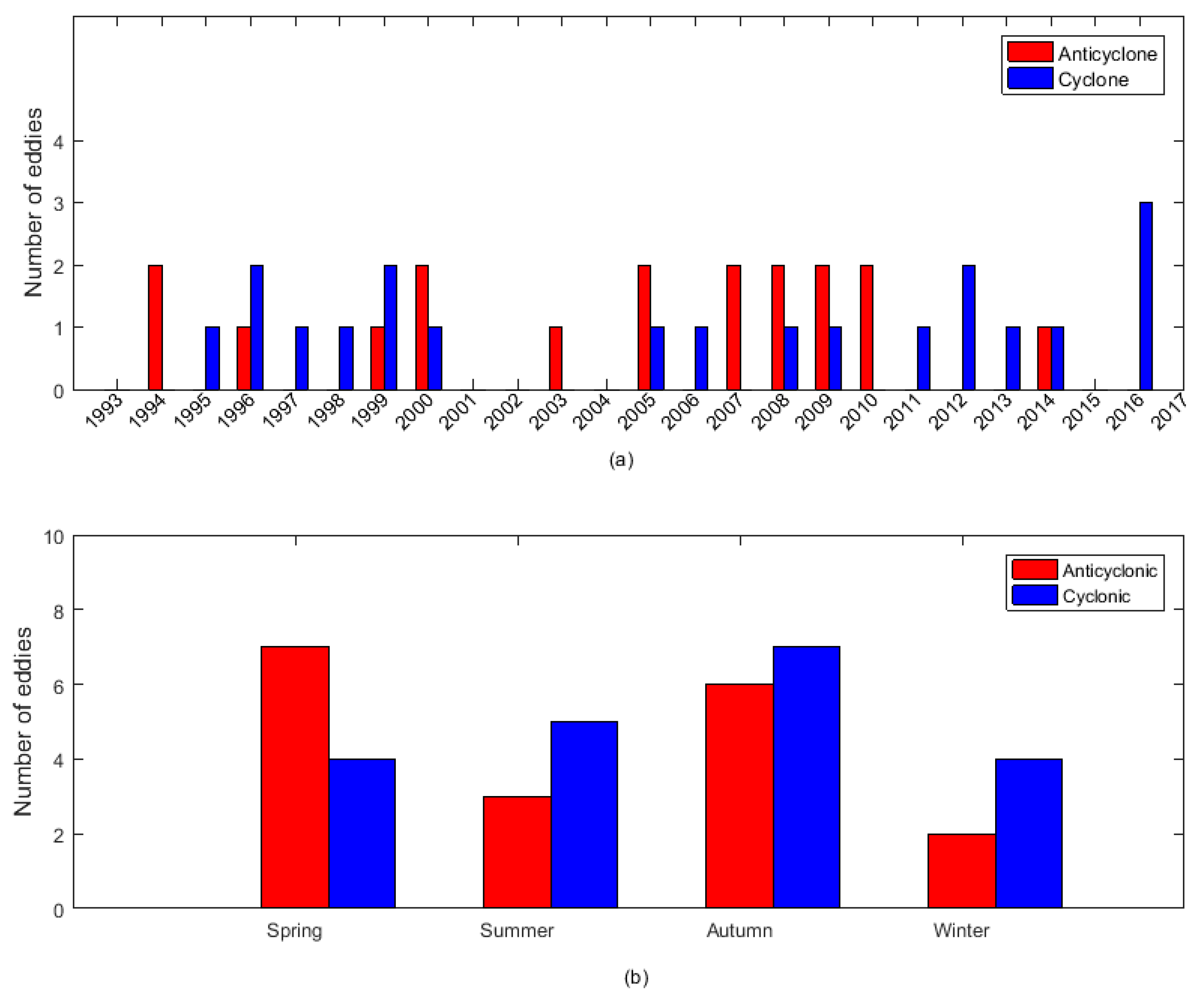
The temporal variability of the local wandering type of mesoscale eddies is shown in Figure 9. One can see that the number of cyclonic mesoscale eddies is greater than the number of anticyclonic eddies of this type. The average number of eddies of this type is one eddy less per year. The maximum number of mesoscale eddies for the local wandering type is during the summer (14). There are two cyclonic eddies during the spring and the winter in 24 years.
According to the characteristic values shown in Table 3, the average survival time of the local wandering mesoscale eddies are 85 days, up to 202 days. The average amplitude is 16.9 cm. The average radius is 149 km.
3.3.4. Shelf-Internal-Generation Type
The shelf-internal-generation type of mesoscale eddies accounts for 19.5% (36) of the total eddies from 1993 to 2016. The pathways are shown in Figure 10. The eddies are generated in the shelf area, then propagate to the southwest along the shelf. Some of the eddies are generated on the west side of the study area, but most of them are generated on the east side.
Figure 11 shows the temporal variability for the shelf-internal-generation type. One can see that a few eddies are generated in the study area each year. The eddies are generated most often during the spring, the summer, and the autumn (9, 11, and 10 occurrences, respectively), and only one anticyclonic eddy is generated during the winter. It seems that cyclonic eddies are more often generated during the summer and the autumn.
According to the characteristic values presented in Table 4, the average survival time of the shelf-internal-generation mesoscale eddies is 74 days, up to 90 days. The average amplitude is 16 cm. The average radius is 146 km.
4. Discussion
4.1. Background Fields
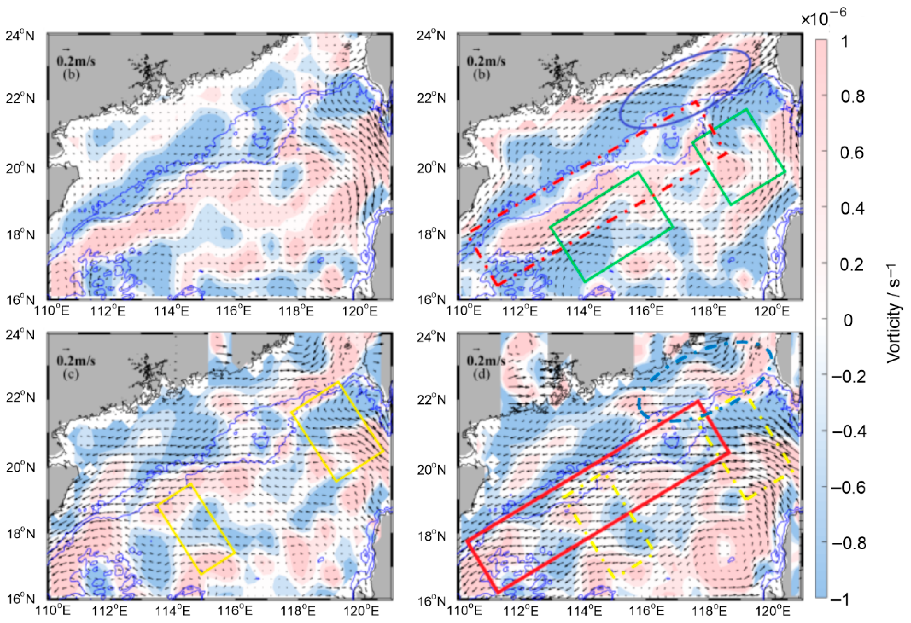
Figure 12 shows the average seasonal variability of the velocity and vorticity fields in the northern SCS derived from the CMEMS current velocities data. As we can see: (1) For the along-the-isobath type the flow on the slope (the dotted red frame in Figure 12b) during the summer is the smallest—less than 0.05 m/s. Meanwhile, the number of eddies in this area is also the smallest for this type. However, the flow in this area (the red frame in Figure 12d) during the winter is larger than 0.1 m/s, and the flow direction is southwest. In this season, half of the eddies spread along the isobaths, namely, southwest. It seems that eddies of this type are impacted by the strong background flow. (2) For the intrusion type, one can see that the eddies invade the continental shelf during the autumn, when the water flows toward the shelf (the yellow frame in Figure 12c). During the winter, few eddies invade the shelf as the flow is strong. (3) For the local wandering type, the small northeast flow during the summer is beneficial to wandering for eddies. (4) For the shelf-generation type, the strong northeast flow during the summer on the shelf (the blue frame in Figure 12b) is beneficial to the generation of the eddies. However, during the winter the southwest flow should inhibited the generation of eddies on the shelf (the blue frame in Figure 12d).
It seems that the flow plays an important role for the eddy pathway. A strong southwestward flow on the slope would carry along the eddies. The eddies would probably invade the shelf, when the strong flow invades the shelf. However, the eddy would probably be generated on the shelf, or be led to wandering by the strong northeastward background flow, during the summer.
4.2. Interaction with Wind and Topography
Besides the upper ocean circulation, wind stress would also induce the Ekman transport. The space–time fluctuations in the Ekman transport would amplify the barotropic component of the total current [26]. The SCS is controlled by the monsoon during the winter and the summer; hence, the along-the-isobath type in this study accounts for 47.3% of the total mesoscale eddies. The intrusion of eddies occurs more often during the spring and the autumn. Moreover, the Ekman current develops in the surface layer, and the differential advection of geostrophic vorticity by the Ekman components tends to tilt the vortex in a vertical direction [27,28]. The three-dimensional structure of the eddies observed by mooring arrays on the slope of the SCS is characterized by a distinct vertical tilt [29]. The tilt phenomenon of the eddy in the vertical direction could not be shown by satellite altimeter data.
The topography produces a restoring mechanism for wave generation, and acts as a wave guide [30]. The eddy would drift towards the escarpment in the cases where the eddy travels in the direction of the topographic wave phase [30]. That is the reason that the intrusion of eddies occurs more often in the northeast of the SCS, where the terrain is steep, and the eddy energy scatters quickly upon encountering the escarpment [31].
5. Conclusions
The statistical characteristics of 184 mesoscale eddies that entered the continental shelf area of the northern SCS from 1993 to 2016 are as follows: (1) the mesoscale eddies exhibit interannual variations with about 3-year cycles, (2) the mesoscale eddies are more likely to enter the shelf of the northern SCS during the autumn (52 occurrences) and the winter (53), with the minimum number (only 35) occurring in spring.
According to their motion paths, we classify the eddies into four types: the along-the-isobath, the intrusion-of-continental-shelf, the local wandering, and the internal-shelf-generation. The number of eddies for the along-the-isobath type peaks during the winter (about 40). The number of anticyclonic eddies is twice as many as the number of cyclonic eddies. The eddies for the intrusion-of-the-shelf type are more likely be detected during the spring and the autumn. Contrary to the along-the-isobath type, the number of eddies for the local wandering type peaks during the summer. The internal generation eddies occur most often during the spring, the summer, and the autumn (9, 11, and 10 occurrences, respectively). The flow plays an important role for the seasonal distribution of eddies.
The mean lifetime, amplitude, and radius of eddies of the internal-generation type is the smallest, about 74 d, 16.0 cm, and 146 km, compared with the along-the-isobath type, which is the largest, about 93 d, 18 cm, and 154 km.
Author Contributions
Conceptualization, J.L.; Investigation, T.Z.; supervision, Q.Z. and L.X.; writing—original draft, T.Z.; writing—review and editing, J.L. All authors have read and agreed to the published version of the manuscript.
Funding
This research was funded by the National Natural Science Foundation of China, grant number 41476009, 41506018, 41976200; Guangdong Province First-Class Discipline Plan, grant number CYL231419012; Innovation Team Plan for Universities in Guangdong Province, grant number 2019KCXTF021; Matched Grant of Guangdong Ocean University, grant number P15299, P17263; the Open Fund of the Key Laboratory of Ocean Circulation and Waves, Chinese Academy of Sciences; Program for Scientific Research Start-up Funds of Guangdong Ocean University.
Institutional Review Board Statement
Not applicable.
Informed Consent Statement
Not applicable.
Data Availability Statement
The mesoscale eddy trajectory product is derived from AVISO (https://www.aviso.altimetry.fr/es/data/products/value-added-products/global-mesoscale-eddy-trajectory-product.html (accessed on 27 January 2022)). The daily mean total surface and 15 m current velocities data product is obtained from the CMEMS (http://marine.copernicus.eu/services-portfolio/access-to-products/?option=com_csw&view=details&product_id=MULTIOBS_GLO_PHY_REP_015_004 (accessed on 27 January 2022)).
Acknowledgments
The authors sincerely thank the anonymous reviewers for their valuable suggestions in improving the manuscript.
Conflicts of Interest
The researchers claim no conflict of interests.
References
- Mc Williams, J.C. Geostrophic Vortices. In Nonlinear Topics in Ocean Physics, Proceedings of the International School of Physics “Enrico Fermi”, Course CIX, Varenna, Italy, 26 July–5 August 1988; North Holland: New York, NY, USA, 1991; pp. 5–50. [Google Scholar]
- Carton, X. Oceanic Vortices. In Fronts, Waves and Vortices in Geophysical Flows; Lecture Notes in Physics; Flor, J.B., Ed.; Springer: Berlin/Heidelberg, Germany, 2010; Volume 805. [Google Scholar] [CrossRef]
- Shang, X.; Xu, C.; Chen, G.; Lian, S. Review on mechanical energy of ocean mesoscale eddies and associated energy sources and wink. J. Trop. Ocean. 2013, 32, 24–36, (In Chinese with English abstract). [Google Scholar]
- Mcdowell, S.E.; Rossby, H.T. Mediterranean Water: An Intense Mesoscale Eddy off the Bahamas. Science 1987, 202, 1085–1087. [Google Scholar] [CrossRef] [PubMed]
- Wang, G.; Su, J.; Qi, Y. Advances in studying Mesoscale eddy in the South China Sea. Adv. Earth Sci. 2005, 20, 882–886. [Google Scholar]
- Chelton, D.B.; Schlax, M.G.; Samelson, R.M.; de Szoeke, R.A. Global observations of large oceanic eddies. Geophys. Res. Lett. 2007, 34, L15606. [Google Scholar] [CrossRef]
- Chelton, D.B.; Schlax, M.G.; Samelson, R.M. Global observations of nonlinear mesoscale eddies. Prog. Oceanogr. 2011, 91, 167–216. [Google Scholar] [CrossRef]
- Le Traon, P.Y.; Morrow, R. Ocean currents and eddies. Int. Geophys. 2001, 69, 171–215. [Google Scholar]
- Zhang, Z.; Zhao, W.; Tian, J.; Liang, X. A mesoscale eddy pair southwest of Taiwan and its influence on deep circulation. J. Geophys. Res. Ocean. 2013, 118, 6479–6494. [Google Scholar] [CrossRef]
- Munk, W.; Armi, L.; Fischer, K.; Zachariasen, F. Spirals on the sea. Proc. R. Soc. Lond. A Math. Phys. Eng. Sci. 2000, 456, 1217–1280. [Google Scholar] [CrossRef]
- Apel, J.R. Principles of Ocean Physics; Academic Press: Orlando, FL, USA, 1987; p. 634. [Google Scholar]
- Liu, Q.; Yang, H.; Liu, Z. Seasonal features of the Sverdrup circulation in the South China Sea. Prog. Nat. Sci. Mater. Int. 2001, 11, 203–206. [Google Scholar]
- Lin, H.; Hu, J.; Zheng, Q. Satellite altimeter data analysis of the South China Sea and the northwest Pacific Ocean: Statistical features of oceanic mesoscale eddies. J. Oceanogr Taiwan Strait 2012, 1, 105–113, (In Chinese with English abstract). [Google Scholar]
- Hu, J.; Zheng, Q.; Sun, Z.; Tai, C.K. Penetration of nonlinear Rrossby eddies into South China Sea evidenced by cruise data. J. Geophys. Res. Ocean. 2012, 117, C03010. [Google Scholar] [CrossRef]
- Zheng, Q.; Hu, J.; Zhu, B.; Feng, Y.; Jo, Y.-H.; Sun, Z.; Zhu, J.; Lin, H.; Li, J.; Xu, Y. Standing wave modes observed in the South China Sea deep basin. J. Geophys. Res. Ocean. 2014, 119, 4185–4199. [Google Scholar] [CrossRef] [Green Version]
- Xie, L.; Zheng, Q.; Zhang, S.; Hu, J.; Li, M.; Li, J.; Xu, Y. The Rossby normal modes in the South China Sea deep basin evidenced by satellite altimetry. Int. J. Remote Sens. 2018, 39, 399–417. [Google Scholar] [CrossRef]
- Huang, R.; Xie, L.; Zheng, Q.; Li, M.; Bai, P.; Tan, K. Statistical analysis of mesoscale eddy propagation velocity in the South China Sea deep basin. Acta Oceanol. Sin. 2020, 39, 91–102. [Google Scholar] [CrossRef]
- Wang, M.; Zhang, Y.; Liu, Z.; Wu, J. Temporal and Spatial Characteristics of Mesoscale Eddies in the Northern South China Sea: Statistics Analysis Based on Altimeter Data. Adv. Earth Sci. 2019, 34, 1069–1080. [Google Scholar]
- Wang, W.; Chen, Q. Warm Heart Vortex in the Northern South China Sea (I). J. Oceanogr. Natl. Taiwan Univ. 1987, 18, 104–113. (In Chinese) [Google Scholar]
- Wang, G.; Xue, H.; Xu, J. Improved inverse model of circulation in the northeastern South China Sea. In Chinese Oceanographic Collection—Numerical calculation of the South China Sea Current and Mesoscale Characteristics; China Ocean Press: Beijing, China, 2001. (In Chinese) [Google Scholar]
- Xiu, P.; Chai, F.; Shi, L.; Xue, H.; Chao, J. A Census of Eddy Activities in the South China Sea during 1993–2007. J. Geophys. Res. Ocean. 2010, 115, C03012. [Google Scholar] [CrossRef] [Green Version]
- Wang, W.; Liu, Y.; Zhu, J.; Shen, J. Seasonal and Interannual Variations of Mesoscale Vortex Intensity in the South China Sea. Mar. Sci. 2016, 40, 94–106, (In Chinese with English abstract). [Google Scholar]
- Shu, Y.; Wang, Q.; Yan, T. Research progress on the continental shelf flow system in the northern South China Sea. Sci. China Earth Sci. 2018, 48, 276–287. [Google Scholar]
- Cheng, X.; Qi, Y.; Wang, W. Analysis of Seasonal and Interannual Variability of Mesoscale Vortex in the South China Sea. J. Trop. Oceanogr. 2005, 24, 51–59, (In Chinese with English abstract). [Google Scholar]
- Li, Y.; Cai, W.; Li, L.; Xu, D. Seasonal and interannual variations of scale vortices in the northeastern South China Sea. J. Trop. Oceanogr. 2003, 22, 61–70, (In Chinese with English abstract). [Google Scholar]
- Stern, M.E. Interaction of a uniform wind stress with hydrostatic eddies. Deep Sea Res. 1966, 13, 193–203. [Google Scholar] [CrossRef]
- Stern, M.E. Interaction of a uniform wind stress with a geostrophic vortex. Deep Sea Res. 1965, 12, 355–367. [Google Scholar] [CrossRef]
- Morel, Y.; Thomas, L.N. Ekman drift and vortical structures. Ocean Model. 2009, 27, 185–197. [Google Scholar] [CrossRef]
- Zhang, Z.; Tian, J.; Qiu, B.; Zhao, W.; Chang, P.; Wu, D.; Wan, X. Observed 3D Structure, Generation, and Dissipation of Oceanic Mesoscale Eddies in the South China Sea. Sci. Rep. 2016, 6, 24349. [Google Scholar] [CrossRef] [PubMed]
- Dunn, D.C. Vortex Interactions with Topographic Features in Geophysical Fluid Dynamics. Ph.D. Thesis, University College London, London, UK, 1999. [Google Scholar]
- Hinds, A.K.; Johnson, E.R.; Mcdonald, N.R. Vortex scattering by step topography. J. Fluid Mech. 2007, 571, 495–505. [Google Scholar] [CrossRef] [Green Version]
Figure 1.
Topographic map of the continental shelf in the northern SCS. The red curve indicates the study area. The numerals on the isobaths are in m.
Figure 1.
Topographic map of the continental shelf in the northern SCS. The red curve indicates the study area. The numerals on the isobaths are in m.

Figure 2.
Histogram of the number of mesoscale eddies in the study area from 1993 to 2016: (a) power spectral density (PSD) of the mesoscale eddy number; (b) red and blue bars in (a) indicate anticyclonic and cyclonic eddies, respectively. The red and blue curves in (b) are for anticyclonic and cyclonic eddies, respectively.

Figure 3.
Seasonal distribution of the number of mesoscale eddies in the study area. The blue and red bars indicate cyclonic and anticyclonic eddies, respectively.
Figure 3.
Seasonal distribution of the number of mesoscale eddies in the study area. The blue and red bars indicate cyclonic and anticyclonic eddies, respectively.

Figure 4.
The pathways of the along-the-isobath type mesoscale eddies. The red curves with points are anticyclonic eddies. The blue curves with points are cyclonic eddies. The circles indicate generation and the asterisks indicate corruption.
Figure 4.
The pathways of the along-the-isobath type mesoscale eddies. The red curves with points are anticyclonic eddies. The blue curves with points are cyclonic eddies. The circles indicate generation and the asterisks indicate corruption.

Figure 5.
(a) Interannual and (b) seasonal distribution of the number of the along-the-isobath type. The red columns indicate anticyclonic eddies, and the blue columns indicate cyclonic eddies.
Figure 5.
(a) Interannual and (b) seasonal distribution of the number of the along-the-isobath type. The red columns indicate anticyclonic eddies, and the blue columns indicate cyclonic eddies.

Figure 6.
The pathways of the intrusion-of-continental-shelf mesoscale eddies. The red curves with points are anticyclonic eddies. The blue curves with points are cyclonic eddies. The circles indicate generation and the asterisks indicate corruption.
Figure 6.
The pathways of the intrusion-of-continental-shelf mesoscale eddies. The red curves with points are anticyclonic eddies. The blue curves with points are cyclonic eddies. The circles indicate generation and the asterisks indicate corruption.

Figure 7.
(a) Interannual and (b) seasonal statistics of the intrusion-of-continental-shelf mesoscale eddies entering the northern shelf of the SCS.
Figure 7.
(a) Interannual and (b) seasonal statistics of the intrusion-of-continental-shelf mesoscale eddies entering the northern shelf of the SCS.

Figure 8.
The pathways of the local wandering mesoscale eddies. The red curves with points are anticyclonic eddies. The blue curves with points are cyclonic eddies. The circles indicate generation and the asterisks indicate corruption.
Figure 8.
The pathways of the local wandering mesoscale eddies. The red curves with points are anticyclonic eddies. The blue curves with points are cyclonic eddies. The circles indicate generation and the asterisks indicate corruption.

Figure 9.
(a) Interannual and (b) seasonal statistics of the local wandering type. The red columns indicate the anticyclonic eddies. The blue columns indicate the cyclonic eddies.
Figure 9.
(a) Interannual and (b) seasonal statistics of the local wandering type. The red columns indicate the anticyclonic eddies. The blue columns indicate the cyclonic eddies.

Figure 10.
The pathways of the shelf-internal-generation mesoscale eddies. The red curves with points are anticyclonic eddies. The blue curves with points are cyclonic eddies. The circles indicate generation and the asterisks indicate corruption.
Figure 10.
The pathways of the shelf-internal-generation mesoscale eddies. The red curves with points are anticyclonic eddies. The blue curves with points are cyclonic eddies. The circles indicate generation and the asterisks indicate corruption.

Figure 11.
(a) Interannual and (b) seasonal statistics of the shelf-internal-generation type. The red columns indicate the anticyclonic eddies. The blue columns indicate the cyclonic eddies.
Figure 11.
(a) Interannual and (b) seasonal statistics of the shelf-internal-generation type. The red columns indicate the anticyclonic eddies. The blue columns indicate the cyclonic eddies.

Figure 12.
The average seasonal variability of the background flow field (arrows) and the vorticity field (colored) in the northern SCS derived from the CMEMS current velocities data during: (a) spring, (b) summer, (c) autumn, (d) winter. The red, yellow, green, and blue frames represent cluster areas for the along-the-isobath type, the intrusion-of-continental-shelf type, the local wandering type, and the shelf-internal-generation type, respectively. The solid and dotted boxes represent the cluster area for the largest and the smallest number of eddies, respectively.


Table 1.
Characteristics of the along-the-isobath mesoscale eddies.
| Characteristic Parameters | Lifetime (d) | Amplitude (cm) | Radius (km) |
|---|---|---|---|
| Value | 93 ± 55 | 18.0 ± 8.0 | 154 ± 43 |
Table 2.
Characteristics of the intrusion-of-continental-shelf mesoscale eddies.
| Characteristic Parameters | Lifetime (d) | Amplitude (cm) | Radius (km) |
|---|---|---|---|
| Value | 82 ± 53 | 17.0 ± 7.4 | 149 ± 41 |
Table 3.
Characteristics of the local wandering mesoscale eddies.
| Characteristic Parameters | Lifetime (d) | Amplitude (cm) | Radius (km) |
|---|---|---|---|
| Value | 85 ± 53 | 16.9 ± 7.8 | 149 ± 41 |
Table 4.
Characteristics of the shelf-internal-generation mesoscale eddies.
| Characteristic Parameters | Lifetime (d) | Amplitude (cm) | Radius (km) |
|---|---|---|---|
| Value | 74 ± 54 | 16.0 ± 7.9 | 146 ± 42 |
Publisher’s Note: MDPI stays neutral with regard to jurisdictional claims in published maps and institutional affiliations. |
© 2022 by the authors. Licensee MDPI, Basel, Switzerland. This article is an open access article distributed under the terms and conditions of the Creative Commons Attribution (CC BY) license (https://creativecommons.org/licenses/by/4.0/).
Share and Cite
MDPI and ACS Style
Zhang, T.; Li, J.; Xie, L.; Zheng, Q. Statistical Analysis of Mesoscale Eddies Entering the Continental Shelf of the Northern South China Sea. J. Mar. Sci. Eng. 2022, 10, 206. https://doi.org/10.3390/jmse10020206
AMA Style
Zhang T, Li J, Xie L, Zheng Q. Statistical Analysis of Mesoscale Eddies Entering the Continental Shelf of the Northern South China Sea. Journal of Marine Science and Engineering. 2022; 10(2):206. https://doi.org/10.3390/jmse10020206
Chicago/Turabian StyleZhang, Tao, Junyi Li, Lingling Xie, and Quanan Zheng. 2022. "Statistical Analysis of Mesoscale Eddies Entering the Continental Shelf of the Northern South China Sea" Journal of Marine Science and Engineering 10, no. 2: 206. https://doi.org/10.3390/jmse10020206
Note that from the first issue of 2016, this journal uses article numbers instead of page numbers. See further details here.