Quantifying Background Magnetic Fields at Marine Energy Sites: Challenges and Recommendations

Abstract

Unknowns around the environmental effects of marine renewable energy have slowed the deployment of this emerging technology worldwide. Established testing methods are necessary to safely permit and develop marine energy devices. Magnetic fields are one potential cause of environmental effects and are created when electricity is generated and transmitted to shore. Further, the existing variation of the background magnetic field at sites that may be developed for marine energy is largely unknown, making it difficult to assess how much additional stress or impact the anthropogenic magnetic field may have. This study investigates two instruments for their ability to characterize the background magnetic fields at a potential marine energy site in Sequim Bay, WA. Based on this evaluation, this study recommends an Overhauser magnetomer for assessing the background magnetic field and demonstrates the use of this sensor at a potential marine energy site.

1. Introduction

Obtaining regulatory permits has historically delayed deployments of marine energy devices, including tidal or riverine current energy converters and wave energy converters. These permitting requirements are intended to prevent injury or mortality of marine animals caused by a variety of environmental stressors [1]. One of these environmental stressors is the electromagnetic field (EMF) created by the device itself and the underwater cables needed to transport the device-generated electricity back to shore. Regulators and stakeholders raise this concern because of the uncertainty about whether the deployed cables underwater may affect mobile and migrating species and affect critical life stages. While EMFs have been created by power transmission cables connecting islands or crossing rivers throughout the history of electricity distribution, their impact on the surrounding ecosystem is still poorly understood. These concerns are not unique to the marine energy industry but apply to any powered devices or cables deployed in the ocean, including those used for offshore wind energy and for telecommunications [2].

EMFs consist of both electric and magnetic fields, which are emitted from a cable when an electrical current passes through it. Cable design typically contains material within the housing sheath that effectively forms a Faraday shield, which keeps the electric field from propagating outward [3]. A magnetic field has no analogous barrier and is typically what is evaluated around new underwater cable installations [4]. Marine energy installations can use either alternating current (AC) or direct current (DC) power to transmit back to shore, with the type of power supply and voltage impacting the strength of the magnetic field. Magnetic fields created by DC are constant in magnitude, while those created by AC oscillate with the AC phase. AC-emitted fields are weaker than DC-emitted fields given the same peak electric current [5].

The types of cables expected to be used in the marine and offshore wind energy industry, as well as telecommunications and power cables currently in use, are known to create magnetic fields that are discernable by EMF-sensitive species [5]. While a variety of marine species, including sharks, crabs, and rays, have been demonstrated to be sensitive to anthropogenically-induced magnetic fields, the long-term effects of these magnetic fields on their life histories and reproductive success remain unknown [4,6]. Further, it is becoming apparent that some EMF-sensitive species are affected by changes in the Earth’s magnetic field, but how, and to what extent, localized changes affect EMF-sensitive species is less clear [6,7]. Several recent studies have investigated the impact of natural and anthropogenic changes in magnetic fields [8,9]. In one such study, geomagnetic drift was attributed to the change in the path Pacific salmon traveled to return to their home river [9]. Two before/after studies of subsea high-voltage direct current (HVDC) cable installations, carrying a maximum of 1300 A and 1500 A, found that sessile species do not appear to be affected by cable placement and they recolonized the habitat disturbed by installation within a few years [10,11]. Magnetic fields observed at the seabed from buried HVDC cables (burial is common for HVDC installations), range between 1 and 100 µT depending on burial depth and cable conductor separation [7]. It has been shown in the lab that magnetic fields above 500 µT (a magnitude plausible within 1 m of a 1000 A DC cable [5]) are capable of negatively impacting crab (Cancer pagarus) [12]. In another study, no impact observed field strengths below 250 µT for this crab species or juvenile lobster (Homarus gammarus) [13].

While no adverse impacts around underwater cables for marine energy in particular have been observed, few in situ studies have investigated the impacts, particularly those on mobile species [14]. The lack of long-term monitoring of cables in situ can, in part, be attributed to the lack of established testing protocols and equipment and has resulted in regulatory concerns and permitting delays for marine energy projects [4]. While some survey methods have been established by Takagi et al., these are designed for the explicit purpose of locating DC cables using flux-gate magnetometers (also known as gradiometers) towed by a vessel [15]. Detection of the magnetic fields of telecommunications cables using these methods has been demonstrated, but it is challenging to measure the fields of low-current AC or DC cables (on the order of 0.1 to 10 A) at a distance greater than 10 m because of external noise on the same order as the cable’s field [16,17].

Measurement of the background magnetic field can address some of these challenges to assessing magnetic fields from subsea cables and has been identified as an important part of measurement campaigns in several recent studies. In a mesocosm study of an offshore wind cable conducted off the coast of Scotland, researchers found that an understanding of the background magnetic field is necessary to assess how organisms respond to the presence of a cable and recommended the use of more standardized methods and sensors for measuring magnetic fields at ocean energy sites [18]. A field experiment measuring the impacts of a HVDC cable on salmon near San Francisco, CA, USA found that sources such as metal structures can alter the combined geomagnetic and cable magnetic field to effectively render the cable invisible [17]. Finally, a field study in Florida found that it was possible to detect magnetic fields generated by an AC power cable using a towed Overhauser magnetometer when the background magnetic field was relatively constant [19]. In all three of these studies, the aim was to measure the signature of cables, but each highlights the importance of background magnetic field surveys. In surveying the literature, studies focusing exclusively on the background magnetic field at local sites were not found.

While the aforementioned studies are not all specific to marine energy, their findings are broadly applicable. To facilitate environmental monitoring of magnetic fields at marine energy sites, an understanding of the background magnetic field is necessary before installation, because natural variation in field strength may be on the same order of magnitude as anthropogenic sources. Subtraction of the background magnetic field from data collected in the presence of anthropogenic magnetic fields may allow for easier detection of, or a clearer measurement of, the signal from a low current (on the order of 10 A) cable or device.

Measurement of the background magnetic field also allows the impact from an underwater cable to be placed in the context of natural magnetic fields. At a given marine energy site, it is essential to understand what signals marine organisms are encountering from natural magnetic fields before drawing any conclusions about the potential impact of a cable. This is complicated by the fact that while Earth’s magnetic field intensity remains stable over the long term, intensity, inclination, and declination can vary spatially and temporally with no apparent pattern at any specific location [20]. Geomagnetic declination is better documented than intensity; in our study region of the Pacific Northwest, it is currently decreasing at a rate of 0.1 degree per year, and it is possible that the background intensity could change year to year.

While the magnetic field of North America has been mapped primarily via aeromagnetic surveys [21], to the authors’ knowledge, small fluctuations at the scale of the impact of a cable suitable for a marine energy device have not been broadly mapped. Aeromagnetic surveys are completed by detecting the magnetic field at the altitude of the aircraft. Over land, altitude can be held relatively constant during flight, while over the ocean, altitude consistency is affected by sea surface elevation. Still, aeromagnetic surveys have been used to detect submarines and other features underwater; therefore, they have applications in the marine environment [22]. The U.S. Geological Survey (USGS) magnetic anomaly survey [21] is interpolated on a grid of 1 km resolution, thus there is a gap in local high-resolution magnetic field data.

To bridge this gap, cost-effective methods for measuring magnetic fields at finer resolutions are necessary. As reported here, we have tested the use of two different sensors for the measurement of background magnetic fields at marine energy sites, as well as a third sensor for improving the certainty of location measurements. Note that the intention of this study is not to investigate methods to detect effects and/or impacts of magnetic fields on receptors (marine organisms). Rather, it is to offer insight and observation around methods and technologies for measuring the elements of the stressor under realistic environmental conditions.

Field surveys were conducted in a small tidal channel with peak currents of approximately 2 m/s to measure the background magnetic field in the study area. Through analysis of the collected data, we evaluate a method for measuring the background magnetic field and identify challenges in doing so. Finally, we provide recommendations, lessons learned, and next steps for assessing the impact of a cable on the background magnetic field.

2. Materials and Methods

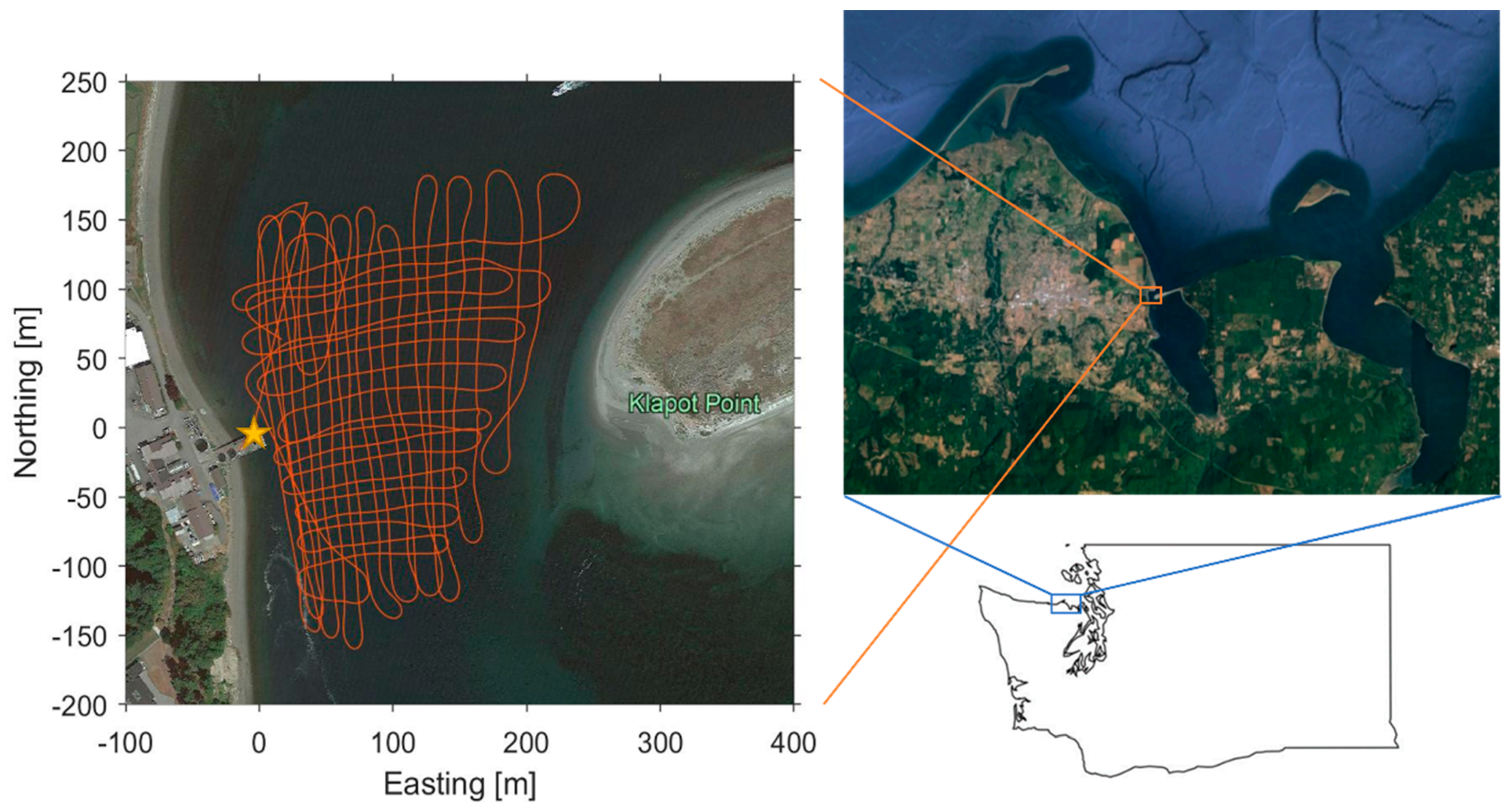
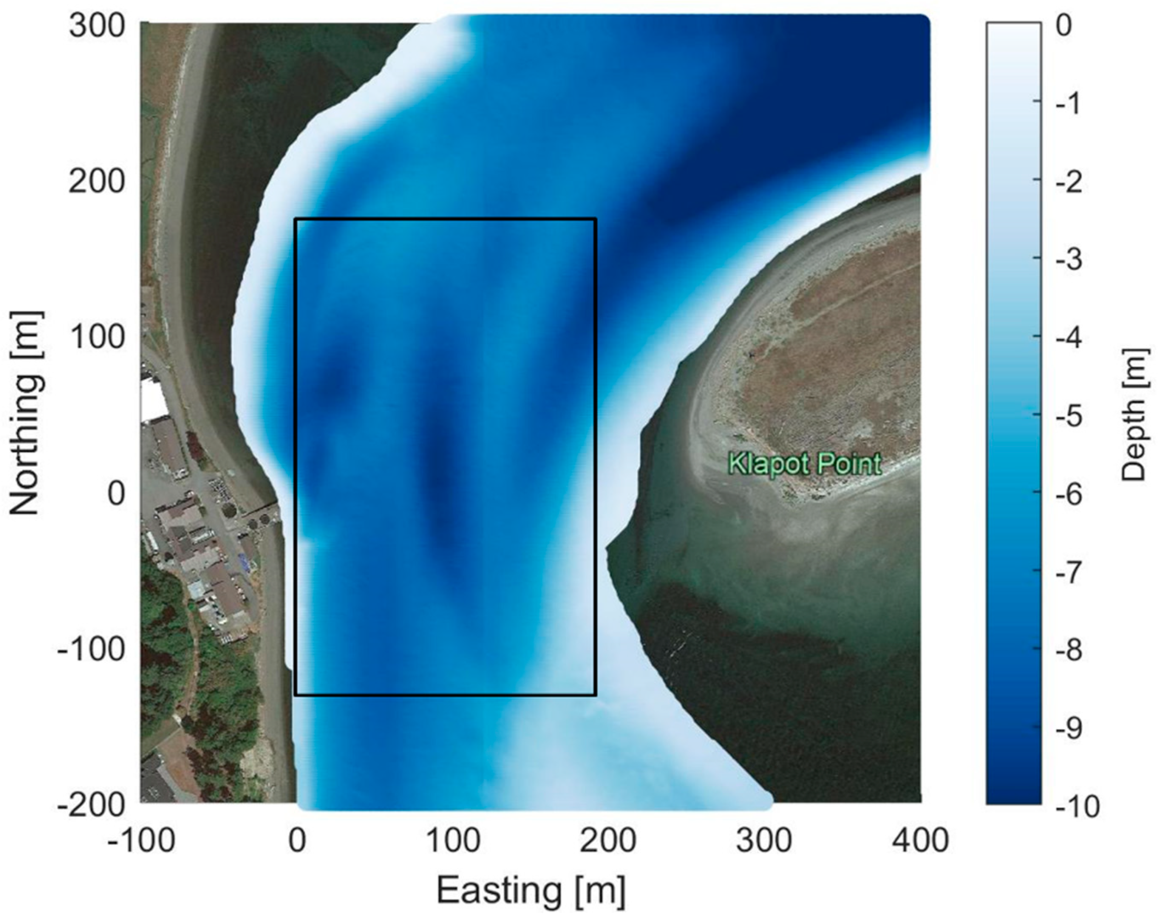
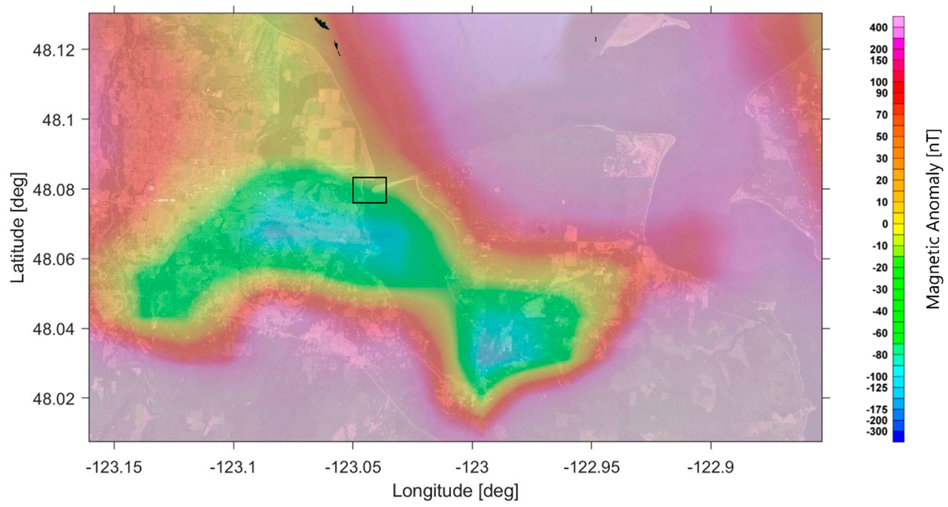
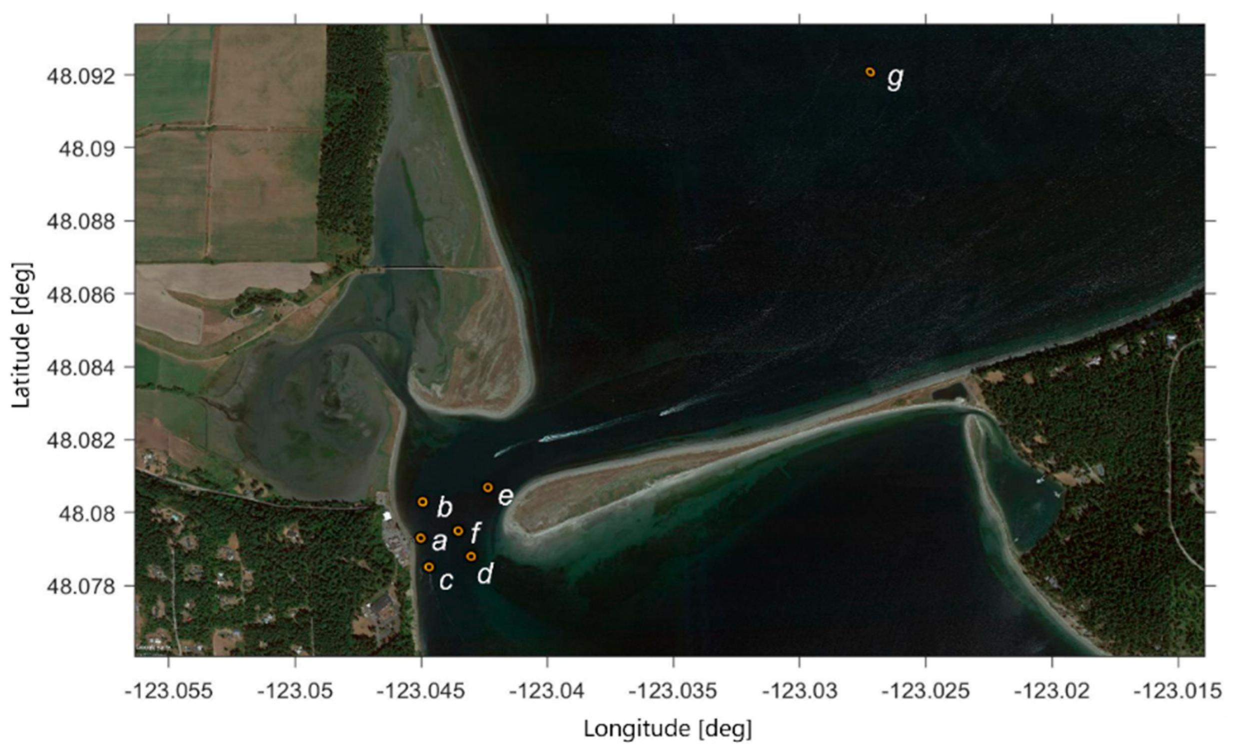
2.1. Study Site

Magnetic field surveys were conducted at the Pacific Northwest National Laboratory’s Marine and Coastal Research Laboratory (MCRL), which sits on 140 acres of tidelands and uplands located on Sequim Bay in Washington State. MCRL is adjacent to the inlet of Sequim Bay, which is proposed for future demonstration installations of tidal turbines. The site features a narrow channel formed by a natural spit (Travis Spit) that separates Sequim Bay from the Strait of Juan de Fuca and experiences tidal currents of up to 2.2 m/s (Figure 1). This channel has maximum depths of 12 m and 8 m under mean higher high water and mean lower low water conditions, respectively. The bathymetry of the site at mean lower low water is shown in Figure 2, in which the undulating seabed can be clearly observed, scoured in certain areas by tidal flow. The survey area focused on the center of the channel directly across from the MCRL dock, which has been identified as the optimal location for a tidal turbine in previous studies [23]. An existing undersea telecommunications cable spans the inlet through the northeast portion of the study site. The sediment of Sequim Bay is predominantly glacial till and has a relatively high iron content, which may serve to amplify or attenuate both the local geomagnetic field and magnetic fields emitted from the electronics equipment. For reference, geomagnetic anomaly data derived from USGS aeromagnetic surveys of the region are shown in Figure 3.

2.2. Instruments for Detecting Magnetic Fields

Two commercially available and relatively economical sensing technologies were evaluated for measuring the magnetic field associated with marine energy systems. The technologies were selected based on their availability, suitability for the marine environment, and anticipated effectiveness for completing the intended mission. First, a total field sensor was chosen—the Marine Magnetics SeaSPY2. The SeaSPY2 is an Overhauser magnetometer, designed to measure the magnitude (vector sum) of the total magnetic field; it is packaged in a small, streamlined tow body and has a sensitivity of 0.1 nT. Advantages of this technology include that it is commercially available, has a low cost relative to custom-built sensors [18], is functional without modifications, includes support from the manufacturer, and comes with softwares for real-time quality assurance. Disadvantages are that it does not resolve field direction and the absolute position of the sensor is hard to determine, because the SeaSPY2 is designed to be towed behind a vehicle using a combined tow/data/power cable. Second, a custom-built sensor capable of measuring the three-dimensional (3D) vector field was evaluated. This system used a Yost TSS-MUSB inertial measurement unit (IMU), which is a microprocessor-based device that has an onboard gyroscope, accelerometer, and a Hall Effect magnetometer. For field measurements, the IMU was enclosed in a protective torpedo-shaped enclosure that could be towed behind the survey vessel. Advantages of this sensor include that it is readily available, has a large user community, is well documented, and can sense the 3D, vector-based magnetic field at a far lower cost than that of equivalent instruments. Disadvantages are that is has significantly lower resolution (73 nT) than Overhauser-based sensors (<1 nT), is not designed to detect magnetic anomalies, and requires customization for use in an underwater environment.

2.3. Magnetic Field Open Water Testing

Both sensor packages were deployed during preliminary testing in July 2020. During this preliminary testing, it was found that the IMU system did not return sensical output, so it was not considered further (see additional discussion under Results). Additionally, after returning the SeaSPY2 to Marine Magnetics for the addition of an altimeter to the sensor package after conducting the 2020 surveys, the manufacturer determined that the sensor hardware was malfunctioning and subsequently repaired and retested the sensor. As a result, data from the 2020 surveys are not shown in this work, but lessons learned during these trials are cited.

Field operations with the repaired SeaSPY2 were conducted 23–25 May 2021 from R/V Desdemona, a 10 m research vessel. Each survey measurement consisted of seven north-south and seven east-west transects, each transect spaced 15 m apart to form an approximately 120 m square grid, as shown in Figure 1. The SeaSPY2 was deployed behind R/V Desdemona by its tow cable, with 20 pounds of lead dive weights attached at the connection point between the tow cable and SeaSPY2 to ensure the sensor remained below the vessel wake.

Transect surveys were conducted during slack water periods between peak tides to maximize the water depth, and hence the area that could be surveyed. Sensor depth was controlled by the length of the deployed tow cable, which was demarcated with tape at 1 m intervals (with “0” located at the SeaSPY2’s magnetometer location), and the speed of the vessel. The sensor was maintained at a specified depth (4 +/− 1 m), rather than at a specified altitude, which was found to be challenging to control in the 2020 field trial because of the variable bathymetry of the site. Sensor depth and altitude were monitored via the SeaSPY2’s altimeter and pressure sensor, and the latter was “zeroed” at the surface each day prior to surveying. To achieve the desired depth, the SeaSPY2 was deployed approximately 15 m behind the vessel traveling at 3 knots on the longer north-south transects and 10 m at 1.5 knots on the shorter east-west transects. Water depth was tracked using the vessel’s depth sounder, which provided advance notice of the undulating bathymetry of the inlet (shown in Figure 2) to avoid collisions of the sensor with the seafloor.

SeaSPY2 data acquisition was controlled with Marine Magnetics’ BOB software, which synchronizes magnetometer readings with the GPS input in real time. The GPS used was an Emlid Reach RS2 GNSS receiver, with standalone accuracy at 0.25 m. Data were collected at 2 Hz, resulting in one measurement on average every 1 m during north-south transects and east-west transects. Sensor distance behind the vessel was determined using the demarcated tow cable plus the known distance between the GPS and vessel stern, which was measured to be 2.5 m horizontally. Readings are therefore only accurate when surveying within transects, not when the vessel turned outside the survey grid, and the data collected while the vessel was turning were removed from the data set before further analysis. The distance behind the vessel was input in the BOB software’s “layback” prompt, which in turn added this displacement distance to the sensor’s GPS record.

It proved difficult to assess the uncertainty of the “layback” method in the 2020 surveys; therefore, to investigate the accuracy of the “layback” method for determining the sensor position, an ultrashort baseline (USBL) system was added to track the position of the SeaSPY2. An AAE Easytrak Nexus Lite USBL was used for this deployment, with an AAE 1219 beacon mounted on the SeaSPY2 at its cable connection. During land-based testing, the beacon was found to interfere with the SeaSPY unless it was mounted directly in line with the magnetometer’s long axis and was fastened in such an orientation at the tow cable connection. The USBL transceiver was mounted over the starboard gunwale of the R/V Desdemona, facing directly downward, 0.75 m below the surface.

Significant variation in the magnetic field with respect to depth was observed during the 2020 survey; therefore, vertical profiles of the magnetic field were taken at various points in the survey grid in 2021, as shown in Figure 4. The SeaSPY2 was loaded horizontally in a sling, lowered gently using the survey boat’s davit until it touched bottom, and lifted back up again. The motors were turned off and the boat was not anchored while taking these measurements. Additionally, during the 2020 field surveys, it was observed that Sequim Bay’s inlet had a potentially high level of magnetic field variability; therefore, an additional vertical profile was taken outside of the inlet toward the Strait of Juan de Fuca to provide context for data collected in the inlet.

2.4. Background Magnetic Field Calculation

All SeaSPY2 survey data collected in 2021 were averaged in a 7.5 m northing by 7.5 m easting by 2 m depth grid to produce an estimate of the background magnetic field. The 7.5 m grid spacing was selected because it is approximately half of the survey grid spacing. Interpolation of the survey transect data across a 3D field was attempted, but interpolation schemes introduced artifacts and discontinuities that were not present in the raw data. While suitable for detecting the location of a cable (e.g., Figure 9 in [7]), interpolation was found to not be ideal for mapping the background field. Additionally, we note that averaging data across the multiple-day field campaign neglects any variability in the magnetic field strength between days. However, an analysis of the data collected on separate days revealed that day-to-day variability was minimal (see

Table 1. Mean absolute difference/mean difference in nT between overlapping data for 3 days of data collection in 2021.

	23 May 2021	24 May 2021	25 May 2021
23 May 2021		11.7/−10.3	13.0/−10.6
24 May 2021	11.7/10.3		6.2/−2.5
25 May 2021	13.0/10.6	6.2/2.5

).

3. Results

3.1. Evaluation of Instruments

The SeaSPY2 measured results matching the existing lower resolution aerial measurements on average, while resolving small scale fluctuations in the magnetic field, demonstrating the instrument’s usefulness in background magnetic field surveys, although determining that the instrument’s horizontal location with sub-meter accuracy proved to be challenging. The SeaSPY2 was able to be towed behind the vessel at a prescribed distance and could maintain depth by adjusting the boat speed or payout of the cable. The USBL was added to the system to increase position accuracy, but the data were noisy, showing the tow body “jumping” tens of meters over several seconds, and the constant layback value almost certainly provided a more accurate position estimate for the tow body. Errors in the USBL data can be attributed to interference from entrained air from the vessel propeller and hull as well as interference with the seafloor in the shallow bay. In a scenario where the marine energy site is in deeper waters and the two-body system would be positioned well below the vessel wake, the addition of this acoustic tracking might be more effective and may be particularly prudent, given that the location of the tow body relative to the vessel may be more variable and difficult to estimate in this scenario. However, it was determined that the simple layback estimation approach is preferable in shallow waters (<10 m) and when operating from small vessels. Using this approach, we conservatively estimated the position uncertainty to be 3 m, which is minor given the resolution of 7.5 m grid spacing, but may not be acceptable for determining the location of an electrified underwater cable.

The Yost IMU evaluated in the preliminary surveys was tested because of its potential to provide vector and high-frequency magnetic field monitoring, as well as to evaluate a lower-cost alternative to the survey-grade commercial instrument. With this focus, the Yost IMU data were initially analyzed for any translational or rotational motions that would interfere with data analysis. The tow body remained steady when traveling through the water, except while turning, and motion readings had an oscillation frequency of 1 Hz, which should have minimal impact on high-frequency measurements. However, the sensor’s magnetic field readings computed as a magnitude did not match the expected (and verified) total natural field centered around 53 µT at any point during operation in 2020, although magnetic field vector directions appeared to be correct. Hypotheses for reasons for the failure of the Yost tow body sensor include the fact that the sensor was not designed to be used in this fashion underwater, possible errors in sensor auto-calibration, water ingress into the sensor enclosure, and/or contamination by and inability to filter magnetic fields from spurious sources.

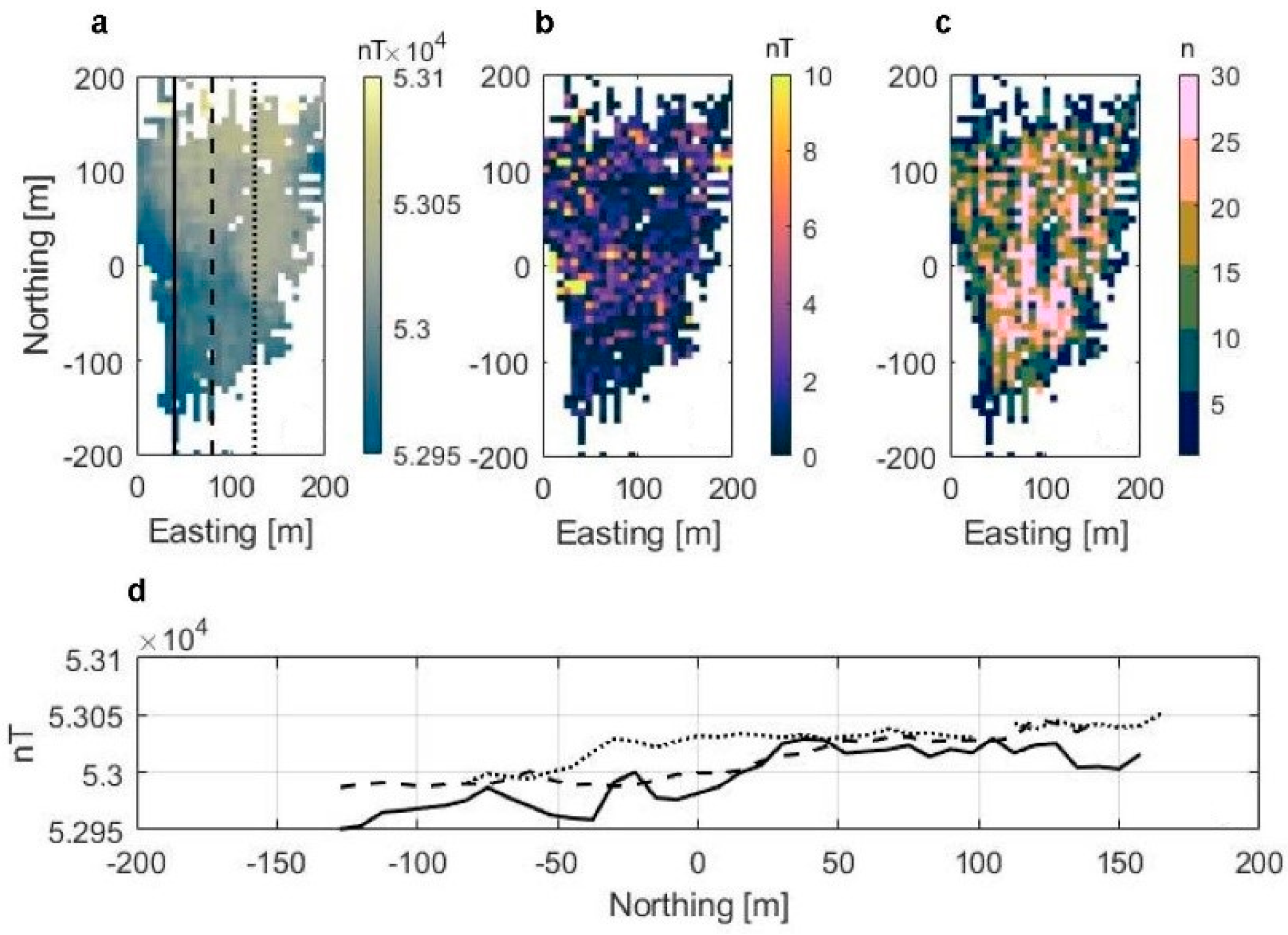
3.2. Background Magnetic Field and Variability

Averaged background data for the vertical bin containing altitudes 6–8 m above the seafloor (approximate mean depth of 4 m), including the standard deviation and number of datapoints in each bin, can be observed in Figure 5. There is an average of seven datapoints in each bin, with an average standard deviation of 1.57 nT. Relatively high bin standard deviations are observed near the MCRL dock, where there was interference from other instrumentation and cables.

Significant variability is observed across the survey area (over 50 nT range), with a relatively high-intensity region observed toward the northeast portion of the study area. Variability in the field follows the local bathymetry elevation in Figure 2. The binned results generally follow geomagnetic anomaly patterns mapped for this area, as shown in Figure 3, with the same magnitude and pattern of magnetic field changes. The higher magnetic field in the northeast corner and lower in the southwest corner follows the aerial surveys.

While the averaged background shows relatively smooth trends across the survey area, the raw, unaveraged timeseries data revealed consistent, significant, anomalies in the magnetic field that are not captured in the background. Figure 6 shows sections of the raw data from three separate north-south transects from the same region of the survey area. Spikes in the magnetic field as high as 100 nT are observed at the same northing in both transects, indicating that they represent anomalies in the magnetic field and are not attributable to sensor noise.

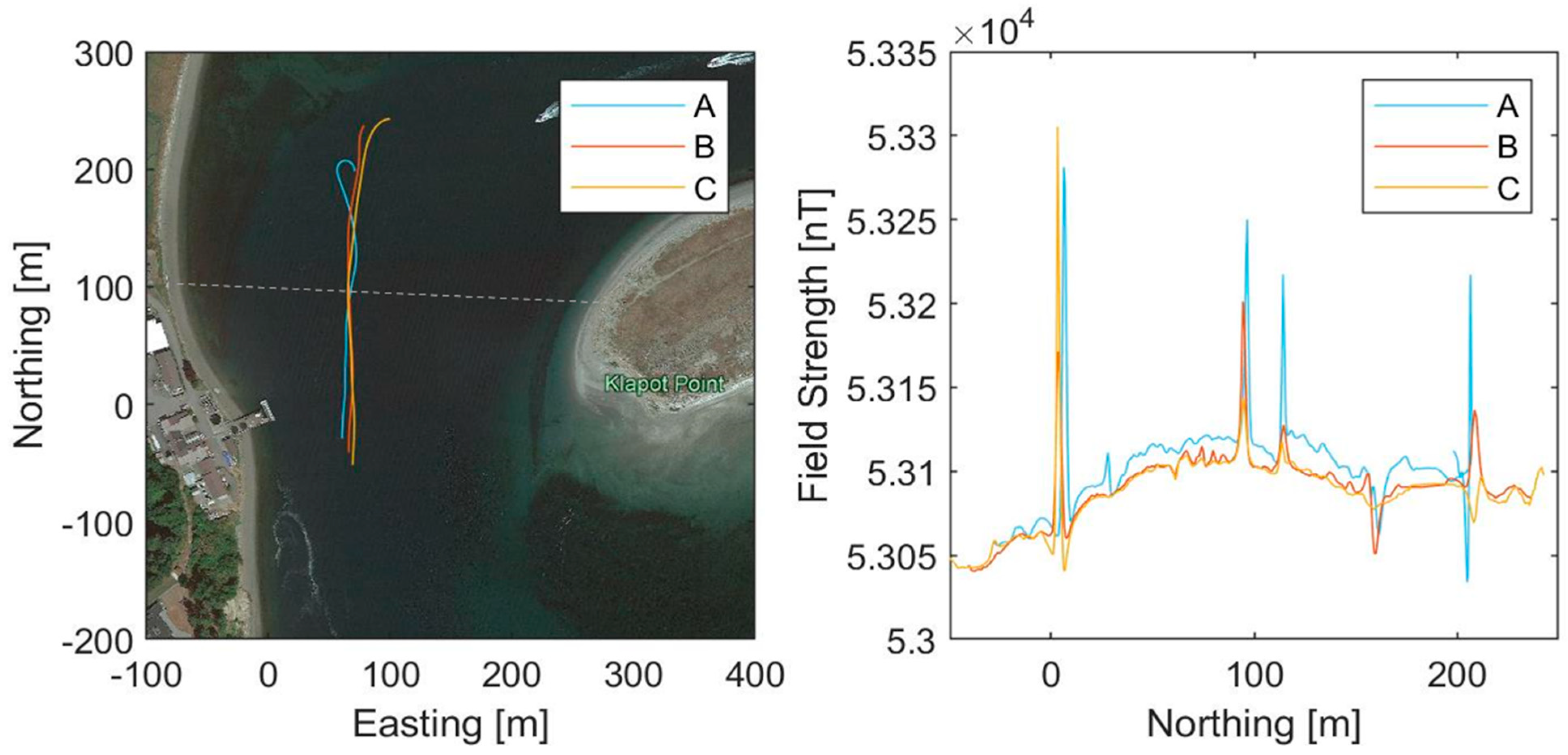
3.3. Background Magnetic Field Compared Day to Day

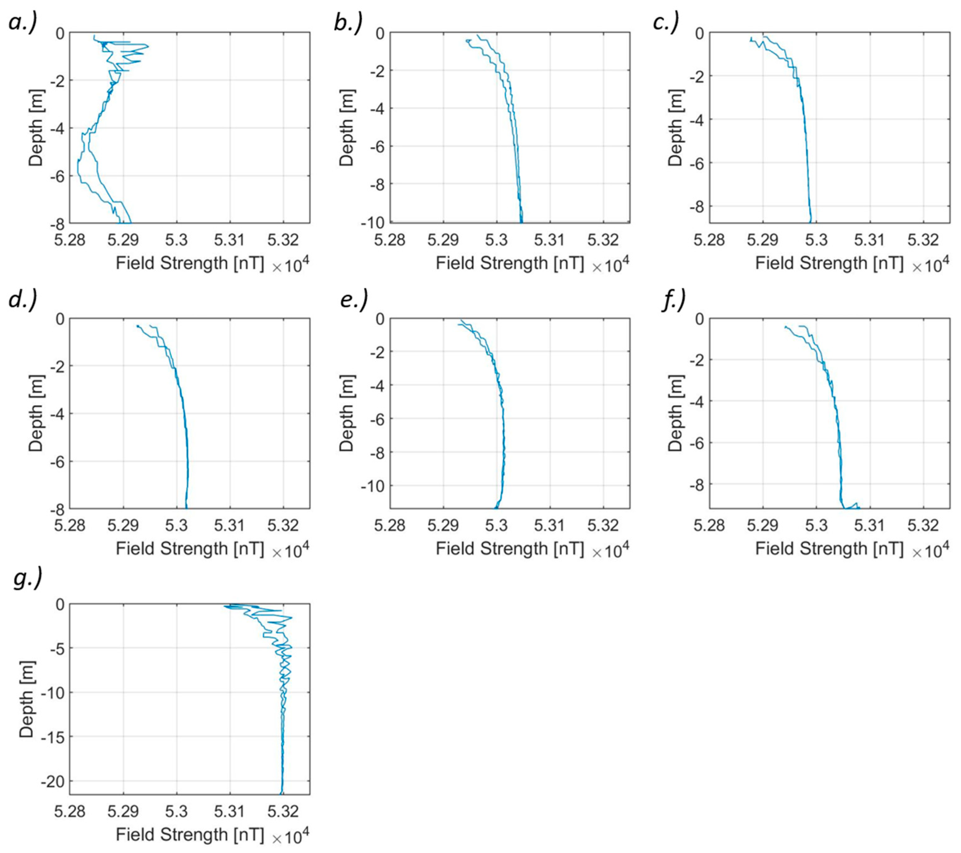
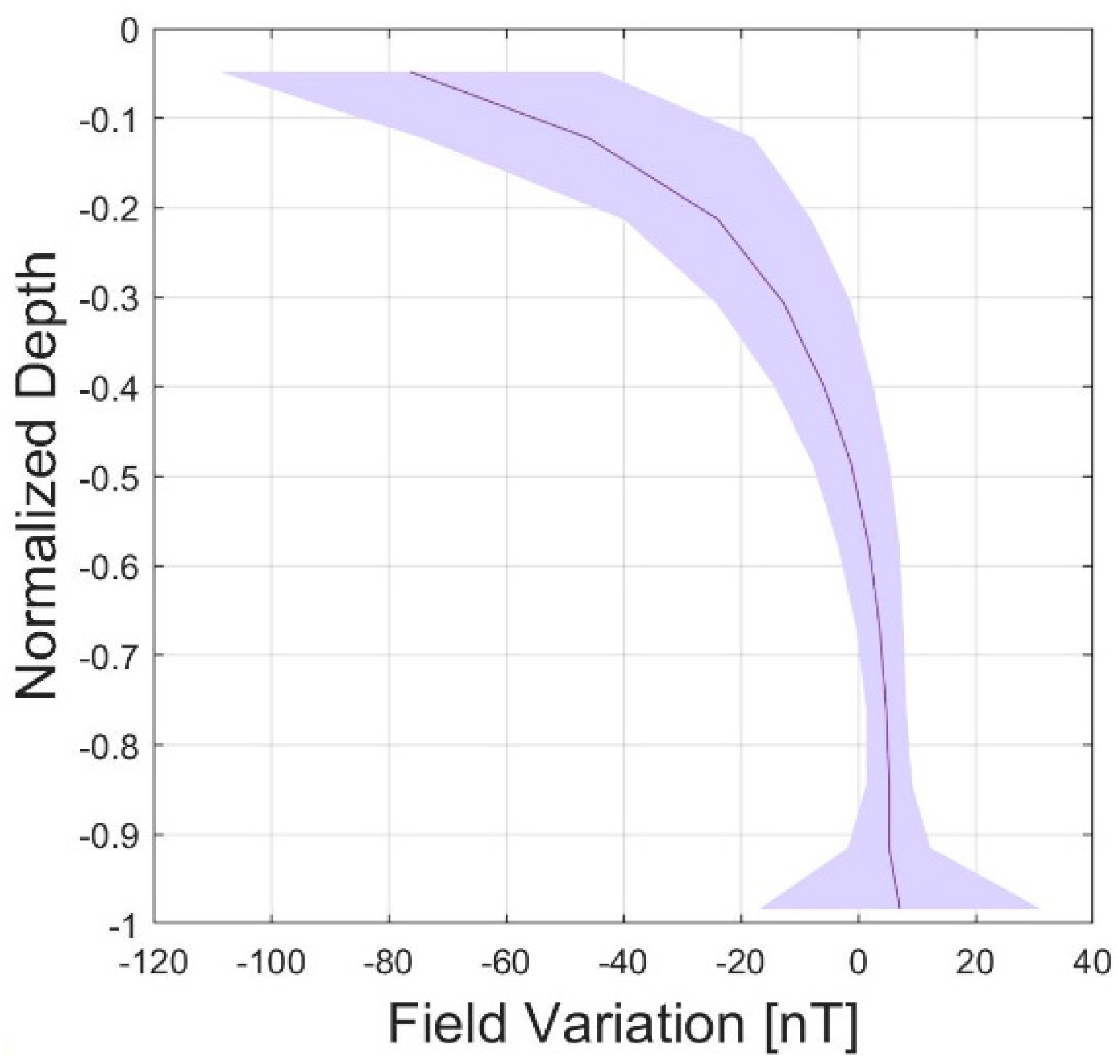
Table 1 shows the mean absolute difference and mean difference between overlapping data in the averaged background when calculated separately for each day of data collection, again presented at an altitude of 6.5 m above the seafloor. As indicated by the mean difference values in Table 1, a general increase in the magnitude of the magnetic field is observed between 23 May 2021 and 25 May 2021, which is more likely attributable to slight changes in the experimental setup day to day (e.g., the sensor was slightly deeper on average or a different number of anomalies were encountered within the 7.5 × 7.5 m bin) or to variable levels of background noise (e.g., passing vessels) than to physical changes in the magnetic field over the course of 3 days. Further, day-to-day variability is significantly lower than the variability across the survey area (Figure 5) and observed anomalies in the magnetic field (Figure 6).

3.4. Depth Profiles

Figure 4 shows the coordinates of the start of each depth profile taken by the SeaSPY2, along with the vessel’s drift distance during the depth profile and the heading of the vessel. Profiles were taken at the end of high slack water when tidal elevation was approximately 2 m above the mean lower low water. The depth profiles are shown in Figure 7. Each profile shows measurements taken both as the instrument was being lowered and as it was being raised, hence the two curves. The difference between these curves at the surface may be attributable to vessel drift because the resulting time difference between surface measurements is greater than that at the seafloor. Increased magnetic field variance observed near the surface in depth profile g, which was taken outside of the tidal channel, was caused by increased wave motion and vessel drift outside the bay. The field strength in profile g was generally of higher intensity than those in the inlet, which conforms with aerial survey data (Figure 3). During depth profile a, the vessel was moored to the MCRL floating dock, which resulted in a near-zero vessel drift. However, the vessel was coupled to the motion of the dock, resulting in increased vertical vessel motion.

The magnetic field intensity is approximately 75 nT weaker at the surface than at depths below 5 m in all locations, except at the MCRL floating dock (point a), where the depth profile is relatively noisy, likely due to the structure of the dock itself and power cables associated with other installed instrumentation. This is in agreement with the higher standard deviations observed near the dock in the bin-averaged survey data observed in Figure 5.

Figure 8 shows the background field variation with depth across the survey area, derived from the average of profiles b−f (all profiles in the survey area, excluding the one taken at the dock) after removing the median from each. The shaded area depicts the maximum and minimum bounds of the profiles b−f and represents a sample of field variation for a profile in the survey area. The range of magnetic field variation at the surface is around 60 nT, which is comparable to that observed in the 1 km aeromagnetic survey data shown in Figure 3. The field is more uniform below depths of 5 m than at the surface, while the field’s rate of change in depths shallower than 5 m best fits a power law and is not the same across profile locations, as observed in the range of variation shown in Figure 8.

4. Discussion

4.1. Recommendations and Guidelines for Background Magnetic Field Testing

The goal of this study is to provide recommendations for characterizing the background magnetic field at a proposed marine energy test site and to demonstrate this in a tidal channel. Our experience and lessons learned can inform future monitoring campaigns. We note that our recommendations are specific to monitoring campaigns using a commercial-off-the-shelf instrument such as the Marine Magnetics SeaSPY2 used here or the Geometrics G-882, towed behind a vessel, remotely operated vehicle, or AUV. While it is an optional feature for the SeaSPY2, we recommend including an altimeter in the sensor package to characterize the distance from the seafloor and to determine the position of the instrument more confidently. An altimeter will be especially useful if both survey area bathymetry and tide levels during the survey are unknown or are known with low resolution. The altimeter can also allow the user to monitor distance from the seafloor in real time to avoid potentially damaging the sensor. Preliminary studies for this effort were completed without an altimeter, leading to more uncertainty in the results, as the altitude was shown to influence the magnetic field at our site (Figure 8).

It was found that measurements at a specified depth are easier to take than at a specified altitude in an area with variable bathymetry. The magnetic field-to-depth relationship was not constant across the survey area but typically shows the same trends from seafloor to surface, because anomalies primarily occur on the seafloor and not in the mid-water column. While existing literature has not observed the background magnetic field to change with depth, the strength of any potential cable will change with the distance away from the cable. At this site, an approximate magnetic field could be generated at multiple depths using the results from Figure 8 to further characterize the magnetic field if that is of interest at a site.

Repeated tests over the course of several days can likely be considered to be part of the same data set. The differences observed in the magnetic field from day to day (Table 1) are unlikely to be resulting from a change in the field day to day, and instead potentially the result of changing tides or slight differences in transect locations. Such differences were not expected on such a short timeframe based on the understood rate of change of Earth’s geomagnetic field. Possible explanations for slight day-to-day variability in the magnetic field are transport of iron-laden sediment by tidal currents or other daily processes, differences in sensor depth smaller than the vertical averaging bin size, and/or testing at different points in the tidal cycle, because the motion of saltwater is known to cause changes in the magnitude of magnetic fields on the order of 1 nT [24]. If background surveys are repeated over months or years, the possibility of measuring changes in the local geomagnetic field intensity should be considered so that they are not inaccurately attributed to marine energy development.

The background magnetic field quantified here resolves anomalies at or larger than the grid resolution (7.5 m²). Anomalies with smaller signatures were smoothed over and skew the mean and standard deviation of their respective grid cells. While the measured background magnetic field could help with identification of the magnetic signatures of later-deployed devices and cables, these original anomalies will still be apparent. Using an AUV with an accurate submarine positioning system (e.g., dead-reckoning with Doppler velocity logging) could help increase the grid resolution and get a more detailed look at the 2D or 3D structure of the field.

4.2. Observations and Limitations from Background Magnetic Field Testing

In these field trials, anomalies in the magnetic field were observed on the orders of 10–100 nT, as seen in Figure 6, while background magnetic field variation of the entire survey area was +/−75 nT. While some previous studies [19] have observed relatively constant background magnetic field levels (+/−5 nT), here we observed fluctuations on the same order of magnitude or higher than may be expected to be associated with a coaxial cable suitable for marine energy transmission.

Field strength from a current-carrying cable can be modeled from the Biot–Savart Law (e.g., [17]):

$$B=\frac{{\mu }_{0}I}{2\pi r}$$

(1)

where B is magnetic field in Teslas, µ₀ is the permeability (taken as 4π × 10⁻⁷ Tm/A), I is the current in amps, and r is the radial distance from the conductor (wire) in meters. For a coaxial cable carrying DC, the magnetic field is influenced by the fact that the power delivery and return path are co-located. If the electric current is the same in both outbound and return paths, then

$$B=\frac{{\mu }_0{I}_{OutboundPath}}{2\pi r_{OutboundPath}}-\frac{{\mu }_0{I}_{ReturnPath}}{2\pi r_{ReturnPath}},$$

(2)

which can be simplified to:

$$B=\frac{{\mu }_{0}I\left(r_{ReturnPath}-r_{OutboundPath}\right)}{2\pi r_{ReturnPath}{r}_{OutboundPath}}$$

(3)

If it is assumed the conductor separation is small relative to the distance r, then

$$B\approx \frac{{\mu }_{0}I\left(r_{ConductorSeparation}\right)}{2\pi r^2}$$

(4)

At a close range to the cable, strong fields will be present, but as the distance increases, the return and outbound paths will be detectable as the sum of fields at the point of the receiver. The sum of the fields is defined by a simple ratio between the radial distance between outbound and return path conductor distances and the measuring device. For a cable with a conductor separation of 25 mm and an electric current of 50 A, characteristic of a cable suitable for power transmission from a single marine energy device, the approximate field strength emitted (from Equation (4)) is shown in

Table 2. Modeled field strength for a representative marine energy transmission cable with a conductor separation of 25 mm and an electric current of 50 A.

Cable
Distance (m)	Field Strength (nT)
1	250
5	10
10	2.5

.

Field strengths in Table 2 combined with the measurements presented in this study indicate that, at some sites, background variability and anomalies in the magnetic field may be strong enough to overpower or “hide” the signal from relatively low power cables. At a distance of 5 m, this example cable’s field (10 nT) is smaller than the background variability observed in the inlet. In addition, the fact that a cable’s magnetic field signature depends on physical cable twist and its orientation to Earth’s field [17,25] could add to the difficulty of identifying a cable. Conversely, we would not anticipate challenges detecting and locating HVDC cables such as those used for subsea power transmission at sites with background variability such as Sequim Bay: the approximately 1000 A of current running through these cables can generate field magnitudes on the order of 1000 nT at 5–10 m range from the cable [5].

4.3. Next Steps in Understanding Magnetic Fields at Marine Energy Sites

Given the variety of cable types and designs, it would be useful to understand the magnetic fields of the types of cables that are likely to be used at MRE sites. For instance, twisted cables, where the conductors are twisted about each other within the cable sheath, emit lower-magnitude fields than the equivalent non-twisted cable because the twist configuration helps cancel each conductor’s field. Understanding the magnetic field signature of different cables can help inform design decisions about cable use and regulatory practices for a given project environment.

A qualitative knowledge of the magnetic field of a project site is necessary to understand the impact of MRE development on marine fauna and the local environment. The magnetic fields of small-scale devices may “blend in” with the background field. In such cases, magnetic fields may not be considered an environmental stressor [1]. However, larger developments may emit fields on the order of HVDC power and communication cables and may require further consideration.

Large knowledge gaps still exist surrounding the impacts and on marine life of submarine cables that are already in the water [14]. The development of consistent methodologies to measure the magnetic field is the first step in closing that gap.

References

1. Boehlert, G.W.; Gill, A.B. Environmental and Ecological Effects of Ocean Renewable Energy Development: A Current Synthesis. Oceanography 2010, 23, 68–81. [Google Scholar] [CrossRef] [Green Version]
2. Copping, A.E.; Hemery, L.G. OES-Environmental 2020 State of the Science Report; Pacific Northwest National Lab. (PNNL): Richland, WA, USA, 2020.
3. Gill, A.B. Offshore Renewable Energy: Ecological Implications of Generating Electricity in the Coastal Zone. J. Appl. Ecol. 2005, 42, 605–615. [Google Scholar] [CrossRef] [Green Version]
4. Gill, A.B.; Desender, M. 2020 State of the Science Report, Chapter 5: Risk to Animals from Electromagnetic Fields Emitted by Electric Cables and Marine Renewable Energy Devices; Pacific Northwest National Lab. (PNNL): Richland, WA, USA, 2020.
5. Normandeau, E.; Tricas, T.; Gill, A. Effects of EMFs from Undersea Power Cables on Elasmobranchs and Other Marine Species; CA OCS Study BOEMRE; U.S. Department of the Interior Bureau of Ocean Energy Management, Regulation and Enforcement Pacific OCS Region: Camarillo, CA, USA, 2011; p. 9.
6. Bonar, P.A.J.; Bryden, I.G.; Borthwick, A.G.L. Social and Ecological Impacts of Marine Energy Development. Renew. Sustain. Energy Rev. 2015, 47, 486–495. [Google Scholar] [CrossRef]
7. Hutchison, Z.L.; Gill, A.B.; Sigray, P.; He, H.; King, J.W. A Modelling Evaluation of Electromagnetic Fields Emitted by Buried Subsea Power Cables and Encountered by Marine Animals: Considerations for Marine Renewable Energy Development. Renew. Energy 2021, 177, 72–81. [Google Scholar] [CrossRef]
8. Cresci, A.; Allan, B.J.M.; Shema, S.D.; Skiftesvik, A.B.; Browman, H.I. Orientation Behavior and Swimming Speed of Atlantic Herring Larvae (Clupea harengus) in Situ and in Laboratory Exposures to Rotated Artificial Magnetic Fields. J. Exp. Mar. Biol. Ecol. 2020, 526, 151358. [Google Scholar] [CrossRef]
9. Putman, N.F.; Lohmann, K.J.; Putman, E.M.; Quinn, T.P.; Klimley, A.P.; Noakes, D.L.G. Evidence for Geomagnetic Imprinting as a Homing Mechanism in Pacific Salmon. Curr. Biol. 2013, 23, 312–316. [Google Scholar] [CrossRef] [PubMed] [Green Version]
10. Andrulewicz, E.; Napierska, D.; Otremba, Z. The Environmental Effects of the Installation and Functioning of the Submarine SwePol Link HVDC Transmission Line: A Case Study of the Polish Marine Area of the Baltic Sea. J. Sea Res. 2003, 49, 337–345. [Google Scholar] [CrossRef]
11. Sherwood, J.; Chidgey, S.; Crockett, P.; Gwyther, D.; Ho, P.; Stewart, S.; Strong, D.; Whitely, B.; Williams, A. Installation and Operational Effects of a HVDC Submarine Cable in a Continental Shelf Setting: Bass Strait, Australia. J. Ocean Eng. Sci. 2016, 1, 337–353. [Google Scholar] [CrossRef] [Green Version]
12. Scott, K.; Harsanyi, P.; Easton, B.A.A.; Piper, A.J.R.; Rochas, C.M.V.; Lyndon, A.R. Exposure to Electromagnetic Fields (EMF) from Submarine Power Cables Can Trigger Strength-Dependent Behavioural and Physiological Responses in Edible Crab, Cancer pagurus (L.). J. Mar. Sci. Eng. 2021, 9, 776. [Google Scholar] [CrossRef]
13. Taormina, B.; Di Poi, C.; Agnalt, A.-L.; Carlier, A.; Desroy, N.; Escobar-Lux, R.H.; D’eu, J.-F.; Freytet, F.; Durif, C.M.F. Impact of Magnetic Fields Generated by AC/DC Submarine Power Cables on the Behavior of Juvenile European Lobster (Homarus gammarus). Aquat. Toxicol. 2020, 220, 105401. [Google Scholar] [CrossRef] [PubMed]
14. Taormina, B.; Bald, J.; Want, A.; Thouzeau, G.; Lejart, M.; Desroy, N.; Carlier, A. A Review of Potential Impacts of Submarine Power Cables on the Marine Environment: Knowledge Gaps, Recommendations and Future Directions. Renew. Sustain. Energy Rev. 2018, 96, 380–391. [Google Scholar] [CrossRef]
15. Takagi, S.; Kojima, J.; Asakawa, K. DC Cable Sensors for Locating Underwater Telecommunication Cables. In Proceedings of the OCEANS 96 MTS/IEEE Conference Proceedings. The Coastal Ocean—Prospects for the 21st Century, Fort Lauderdale, FL, USA, 23–26 September 1996; Volume 1, pp. 339–344. [Google Scholar] [CrossRef]
16. Szyrowski, T.; Sharma, S.K.; Sutton, R.; Kennedy, G.A. Developments in Subsea Power and Telecommunication Cables Detection: Part 2—Electromagnetic Detection. Underw. Technol. 2013, 31, 133–143. [Google Scholar] [CrossRef]
17. Kavet, R.; Wyman, M.T.; Klimley, A.P. Modeling Magnetic Fields from a DC Power Cable Buried Beneath San Francisco Bay Based on Empirical Measurements. PLoS ONE 2016, 11, e0148543. [Google Scholar] [CrossRef] [PubMed] [Green Version]
18. Gill, A.B.; Huang, Y.; Gloyne-Philips, I.; Metcalfe, J.; Quayle, V.; Spencer, J.; Wearmouth, V. COWRIE 2.0 Electromagnetic Fields (EMF) Phase 2: EMF-Sensitive Fish Response to EM Emissions from Sub-Sea Electricity Cables of the Type Used by the Offshore Renewable Energy Industry; Report No. COWRIE-EMF-1-06; Collaborative Offshore Wind Research into the Environment (COWRIE): Cranfield, UK, 2009; p. 68.
19. Dhanak, M.; An, E.; Couson, R.; Frankenfield, J.; von Ellenrieder, K.; Venezia, W. Magnetic Field Surveys of Coastal Waters Using an AUV-Towed Magnetometer. In Proceedings of the 2013 OCEANS—San Diego, San Diego, CA, USA, 23–27 September 2013; pp. 1–4. [Google Scholar] [CrossRef]
20. Hulot, G.; Finlay, C.C.; Constable, C.G.; Olsen, N.; Mandea, M. The Magnetic Field of Planet Earth. Space Sci. Rev. 2010, 152, 159–222. [Google Scholar] [CrossRef]
21. Bankey, V.; Cuevas, A.; Daniels, D.; Finn, C.A.; Hernandez, I.; Hill, P.; Kucks, R.; Miles, W.; Pilkington, M.; Roberts, C.; et al. Digital Data Grids for the Magnetic Anomaly Map of North America; Open-File Report; U.S. Geological Survey: Reston, VA, USA, 2002.
22. Ekinci, Y.L. On the Drape and Level Flying Aeromagnetic Survey Modes with Terrain Effects, and Data Reduction between Arbitrary Surfaces. Turk. J. Earth Sci. 2021, 30, 409–424. [Google Scholar] [CrossRef]
23. Cavagnaro, R.J.; Thomson, J.; Dillon, T.; Stewart, A.; Wang, T.; Yang, Z. Survey and Numerical Model Analysis for Siting Kilowatt-Scale Tidal Turbines. In Proceedings of the 13th European Wave and Tidal Energy Conference (EWTEC 2019), Napoli, Italy, 31 August–6 September 2019. [Google Scholar]
24. Manoj, C.; Kuvshinov, A.; Maus, S.; Lühr, H. Ocean Circulation Generated Magnetic Signals. Earth Planets Space 2006, 58, 429–437. [Google Scholar] [CrossRef] [Green Version]
25. Tchernychev, M.; Johnston, J.; Johnson, R.; Tryggestad, J. Total Magnetic Field Signatures over a Submarine HVDC Cable. In Proceedings of the American Geophysical Union, Fall Meeting, San Francisco, CA, USA, 9–13 December 2013. [Google Scholar]
Figure 1. Sequim Bay field site, with transect lines from a survey run. The yellow star represents the MCRL dock location, which corresponds to 0, 0 Northing and Easting.
Jmse 10 00687 g001
Figure 2. Sequim Bay inlet field site bathymetry. Depth is referenced to MLLW. The MCRL dock is located at (0, 0), which corresponds to (44°04′45.5″ N, 123°02′42.5″ W). The survey area is outlined by the black box.
Jmse 10 00687 g002
Figure 3. Magnetic anomaly map of Sequim Bay and surrounding region, as measured using gradiometers. Data from United States Geological Survey (https://mrdata.usgs.gov/magnetic/map-us.html#home, accessed on 15 April 2022) [21]. Survey area is indicated by the black outline.
Jmse 10 00687 g003
Figure 4. Vertical profiles of the magnetic field relative to the distance from the seafloor were taken at six points in the survey area, including one out toward the Strait of Juan de Fuca.
Jmse 10 00687 g004
Figure 5. (a) Averaged background magnetic field using data from all magnetometer transects at the 6–8 m altitude. (b) The standard deviation of magnetic field samples in each bin. (c) The number of magnetic field samples, n, in each bin. (d) Bin-averaged data at x = 40, 80, and 125 m from the MCRL dock highlight variability across the survey area (shown in Figure 2). Line patterns correspond to the lines in (a). Note that the origin (0, 0) of all plots corresponds to the position of the MCRL dock.
Jmse 10 00687 g005
Figure 6. Example transect data demonstrating consistent magnetic field anomalies. Altitude ranges between 3–5 m across the three transects shown. The telecommunications cable expected location is marked by the dashed gray line. The MCRL dock is located at (0, 0) m, and telecommunications cable(s) are likely causing the anomalies around 100 m North. No devices or instrumentation were deployed by MCRL while this survey was being conducted.
Jmse 10 00687 g006
Figure 7. Depth profiles at locations in Figure 4. The two lines in each profile are measurements from the downcast and upcast (ag). One profile was taken at each location.
Jmse 10 00687 g007
Figure 8. Magnetic field variation versus depth, with maximum and minimum bounds for profiles b–f, specified in Figure 4.
Jmse 10 00687 g008