Long-Term and Seasonal Trends in Global Wave Height Extremes Derived from ERA-5 Reanalysis Data

Abstract

A non-stationary extreme value analysis of 41 years (1979–2019) of global ERA5 (European Centre for Medium-Range Weather Forecasts Reanalysis) significant wave height data is undertaken to investigate trends in the values of 100-year significant wave height, $H_s^{100}$. The analysis shows that there has been a statistically significant increase in the value of $H_s^{100}$ over large regions of the Southern Hemisphere. There have also been smaller decreases in $H_s^{100}$ in the Northern Hemisphere, although the related trends are generally not statistically significant. The increases in the Southern Hemisphere are a result of an increase in either the frequency or intensity of winter storms, particularly in the Southern Ocean.

1. Introduction

The investigation of temporal (long-term and seasonal) and spatial variabilities of metocean parameters, such as the significant wave height, $H_s$, is of significant importance, especially in times of climate change. Long-term changes in oceanic winds, and the waves they generate potentially have important implications for coastal and offshore engineering, coastal flooding and shoreline erosion, shipping and ship routing and the physics of air-sea interaction and climate change.

Studies of trends in mean and upper percentile values of wave height over the last 41 years have been undertaken using in-situ buoy data [1,2,3], hindcast and reanalysis models [3,4,5,6] and satellite remote sensing data [2,7,8]. These studies show small increases in mean significant wave height and stronger increases in upper percentiles over the last 30 years. These trends vary regionally with the largest increases in the Southern Hemisphere. Future projections of global values of mean $H_s$ using ensembles of wave models forced by climate model winds [5] also project that mean conditions will increase in the future, particularly in the Southern Ocean.

Although changes in mean and upper percentile $H_s$ are important, it is the changes in extreme values (e.g., 100-year return period) which are critical for engineering applications. Determination of changes in such statistical values, both for the historical period and for future projections, is challenging both for measurement systems and models. Young et al. [9] attempted to estimate changes in the 100-year return period wind speed and significant wave height over the historical period of satellite altimeter data (25 years). Although there was significant variability in the resulting trends, the results suggested there had been a positive trend in extremes over the period of the data. Projections of changes by 2100 for 100-year return period $H_s$ were undertaken by Meucci et al. [10], using an ensemble of climate models. They found increases in the Southern Ocean of between 5% and 10% over this period.

Extreme Value Analysis (EVA) which is used to estimate, for example, 100-year return period values, traditionally involves the analysis of a time series of values which is assumed stationary. That is, there is no significant trend over the duration of the time series. In order to reduce the confidence limits on the estimated values, it is desirable to have as long a time series as possible. These two requirements potentially conflict, particularly in a period of climate change. That is, as the time series increases in duration, the likelihood that it is stationary decreases. As a result, a range of alternative approaches has been used in an attempt to address the issues and obtain statistically significant results from shorter time series. These approaches include: fitting the extreme value probability distribution to all the data rather than just extremes (the Initial Distribution Method) [11] and “pooling” data from either an ensemble of model results [12,13] or over adjacent spatial regions [14]. A further approach is to relax the requirement that the time series is stationary and undertake a non-stationary extreme value analysis [15].

Long-duration reanalysis datasets which assimilate altimeter data into model hindcasts, such as ERA5 [16], have been shown to have skill in estimating extreme $H_s$ [13]. In this study, we apply a non-stationary extreme value analysis [15] to ERA5 data over the period 1979–2019 to determine global distributions of the 100-year return period significant wave height and also estimate trends in these extreme values over this period. We believe this is the first such study that has applied a widely accepted EVA approach to the estimation of changes in historical extreme value $H_s$.

The arrangement of the paper is as follows. Following this Introduction, Section 2 provides a brief review of extreme value analysis applied to ocean waves, including non-stationary approaches. The datasets used and the approaches applied are described in Section 3, followed by the results in Section 4. The results are discussed in Section 5, followed by conclusions in Section 6.

2. Background

2.1. Extreme Value Analysis

The aim of Extreme Value Analysis (EVA) [17,18] is to estimate the probability distribution function (pdf) of extreme value measurements from a recorded/modelled record. As noted above, the record must be stationary, and the observations in the record should be independent [18]. In the context of estimates of extreme significant wave height, independence is usually achieved by ensuring there are not multiple observations from the same storm event. The requirements that datasets are both stationary and contain only independent observations generally result in relatively short data records (less than 20 years) and large confidence intervals for estimated extreme values. Therefore, a common engineering approach is to relax the requirement that the data are independent and fit a pdf to all observed data. In the case of in-situ buoy data, this may involve observations separated by as little as 1 to 3 h. This approach was termed the Initial Distribution Method (IDM) and typically fitted either a Gumbel or Weibull distribution to the data [19]. In addition to violating the requirement for independent data, as the pdf is fitted to all data rather than only extremes, the resulting estimates tend to largely follow spatial distributions of mean values rather than true extremes. Despite these limitations, the approach has been widely applied for studies of the global distribution of wave height extremes [11,20]. As demonstrated by Takbash et al. [21], however, the limitations of this approach are significant and can result in quite misleading conclusions. In addition, now that both satellite and model datasets span more than 30 years, the need to rely on such approximations no longer exists.

A common approach to ensure that the dataset truly represents extreme values and that the data are independent is to consider annual maximum (AM) values. For such “block maxima”, it can be shown that the values will follow a Generalized Extreme Value (GEV) distribution [18,22]

$$F(H_s)=\exp \left\{-{\left[1+k\left(\frac{H_s-A}{B}\right)\right]}^{-1/k}\right\}$$

(1)

where $F(H_s)$ is the cumulative distribution function form of the GEV and $k,A,B$ are shape, location and scale parameters, respectively. Equation (1) can be used to determine the value of $H_s$ at the desired probability of exceedance, that is, $P(H<H_s^{100})=0.01$, for a 100-year return period event.

Although the AM method has the advantage of ensuring the data are independent, as there is only one value per year, the available data to fit Equation (1) are limited, resulting in large confidence limits for estimates of extreme values. A common method to overcome this limitation is to use a Peaks-over-Threshold (PoT) approach, where all independent peaks above a defined threshold are used. In this case, data can be shown to follow a Generalized Pareto Distribution (GPD) [18]

$$F(H_s)=1-\left[1+k{\left(\frac{H_s-A}{B}\right)}^{-1/k}\right]$$

(2)

where $A$ is the value of the threshold above which data are acquired. There are no rigorous means of determining the value of the threshold other than that it must be sufficiently high to ensure the data are from genuine storms but not so high that there are too few data to fit the GPD form (Equation (2)). PoT approaches have been widely used for global assessment of $H_s^{100}$ [10,11,12,13,14,21].

2.2. Non-Stationary Extreme Value Analysis

As outlined by Mentaschi et al. [15], there are a number of approaches which have been used in an attempt to address the requirement for stationarity outlined above. A common approach is to represent the parameters in Equations (1) and (3) by time-varying parametric functions [23,24,25,26]. The limitation of this approach is that there is no generally accepted method for determining the form of the parametric functions. There has also been a range of approaches which adopt Bayesian methods [27,28]. Further procedures recognize that multivariates of compound approaches, in which extremes may be a function of multiple physical processes, are appropriate [29,30,31,32,33]. Regional or nearshore extremes have also been analyzed using non-stationary approaches [34]. Another method is to divide the non-stationary time series into a series of quasi-stationary slices. The process is termed “stationary of slice” and has been used in a number of studies of climate impacts on metocean parameters [9,10].

Mentaschi et al. [15] proposed an alternative approach called transformed stationary (TS) extreme value analysis. The TS approach involves three separate steps: (i) transform the non-stationary time series, $y(t)$ into a stationary time series, $x(t)$, (ii) apply traditional EVA as outlined above to the transformed time series, (iii) reverse transform the results back to a non-stationary extreme value distribution. Mentaschi et al. [15] proposed that the transformation from $y(t)$ to $x(t)$ could be represented as:

$$x(t)=\frac{y(t)-T_y(t)}{S_y(t)}$$

(3)

where $T_y(t)$ and $S_y(t)$ are the trend and standard deviation of the non-stationary time series, respectively. The transformation represented by Equation (3) ensures that $y(t)$ has a constant mean of zero and a variance of one. Constant mean and variance are necessary conditions for the stationarity of the transformed time series but do not guarantee that this is the case. Therefore, Mentaschi et al. [15] suggest a further test, such as ensuring that higher-order statistics such as kurtosis and skewness are reasonably constant as a function of time for $y(t)$.

Although the approach does require decisions as to how to transform the non-stationary time series to a stationary version (as shown in Equation (3)), it overcomes the significant assumptions required for the alternative approaches described above.

3. Materials and Methods

3.1. ERA5 Global Reanalysis Data

ERA5 is a global reanalysis dataset, constructed by the European Centre for Medium-Range Weather Forecasting (ECMWF) [16]. For this reanalysis, the ERA5 wind fields were used to drive the WAM (WAve Model) with Source Term 3 (ST3) physics [35]. The model also assimilated large amounts of altimeter data into the wave hindcast [36]. The ERA5 values of $H_s$ were downloaded on an 0.5° × 0.5° global grid for the 41-year period from 1 January 1979 to 31 December 2019. To reduce computational expense, the data were used at 1° × 1° resolution, by considering only every second point in the grid, and the TS method was applied at each global grid point. ERA5 has been extensively adopted as a global dataset for wind, wave and other conditions. Although the 0.5° resolution is generally adequate in deep water conditions, and the reanalysis dataset has been validated in a range of studies [16], the data are clearly limited in coastal regions and for relatively small meteorological systems, such as tropical cyclones (see Section 4.1). As such, caution should be exercised in applying the present results in such areas.

3.2. TS EVA Application

The TS EVA approach can be performed using a stationary GEV (Equation (1)), a stationary GPD [Peaks-over-Threshold application (PoT)] (Equation (2)), or any other EVA methodology. As demonstrated by Coles [18], annual maximum data will theoretically follow a GEV distribution, whilst peaks-over-threshold data will follow a GPD. As the peaks-over-threshold approach retains more extreme data than the annual maximum method, and has previously been demonstrated to work well in global applications [21], we adopt this approach. It is not uncommon in EVA applications to test alternative pdfs to the theoretical GPD and determine the best fitting form. As our application is global, such an empirical approach is not feasible. Hence, for the present application, we adopted a GPD approach for all global locations, as described by Mentaschi et al. [15] [see their Equations (19)–(21) and (28)–(30)]. To ensure the data are independent, we required storm-peaks in the PoT analysis to be separated by a minimum of 48 h [12,13,14].

The TS method typically removes the non-stationarity by subtracting the time-varying mean and normalizing the data with the standard deviation of the record (Equation (3)). Running averages of both quantities were used for this purpose. The selection of the time window for the running mean allows both a non-seasonal and seasonal approach to be applied. In the present study, the long-term statistics were determined by setting the non-seasonal time window to five years, and the seasonality was evaluated with the implementation of an additional seasonal time window of two months. Selection of these time windows requires some informed judgement. The non-seasonal window must be long enough to remove the annual variation (multiple years) but not so long that it may remove interannual variability (e.g., El Nino, etc.). A number of values were tested and consistent with Mentaschi et al. [15], the value of five years was adopted. The seasonal window must be long enough to filter out individual weather events but short enough to still resolve the annual cycle (less than a year). For these reasons, a value of two months was adopted. Therefore, the long-term non-seasonal $H_s^{100}$ could be determined from 1979 to 2019 at 5-year intervals. To explore the impacts of seasonality on $H_s^{100}$, the extremes could be derived over the same period but on a monthly basis. For instance, the values of $H_s^{100}$ could be determined for the Northern Hemisphere winter extremes (January), and Southern Hemisphere winter extremes (July). These time windows are consistent with the recommendations of Mentaschi et al. [15].

In order to apply the TS method with a PoT GPD pdf, it is necessary to define the threshold value, $A$ in Equation (2). It is common practice to set this parameter as a percentile value, such that it can dynamically scale for regions with differing wave climates [11,21]. As discussed below, a variety of different thresholds between the 70th and 90th percentile values were tested. To ensure that peaks above the threshold represented independent events, a condition that peaks be separated by 48 h in time was set. It should also be pointed out that the present analysis uses only the threshold value to define storms. Approaches which use additional parameters such as peak wave frequency to define storm events were not considered feasible at the global scale of the present application.

3.3. Trend Estimation

The TS EVA described above enables estimates of the non-seasonal and seasonal (January and July) values of $H_s^{100}$ to be determined at any desired date over the period from 1979 to 2019. Our aim is to estimate $H_s^{100}$ at each global grid point and at regular intervals of time and then undertake trend estimates of the 41-year period. Such a process is computationally expensive, requiring a reasonable investment in super-computing resources. Noting that the trend is slowly varying, $H_s^{100}$ was estimated at 5-year intervals, which is also consistent with the non-seasonal time window adopted. There is significant literature on the estimation of trends [4,7,9,37,38]. Much of these analyses relate to the determination of trends for data which have a significant seasonal signal or where the pdf of the variable does not correspond to a normal distribution. In the present case, the data consist of estimates of $H_s^{100}$ at 5-year intervals. That is, a total of 9 values, over the period from 1979 to 2019, for each non-seasonal and seasonal (January and July) analysis. As a result, simple linear regression was applied [9]. To test the Goodness of Fit (GoF) and the statistical significance of the calculated trends, values of the correlation coefficient, $R^2$ and the p-value were also determined for each grid point. In the results presented below, we highlight trends which are statistically significant at the 95% level based on their p-values.

As will subsequently be shown in Section 4 (Figure 1), the mean trend is not necessarily monotonically increasing (decreasing). Although this is often clear for mean values [7,8], our interest lies in the tail of the pdf where statistical variability increases. As a result, it was not feasible to investigate how the trend varied over the 41-year period. Rather, the linear (least squares) approximation over the full period was deemed consistent with the statistical variability of the EVA estimates.

4. Results

The TS EVA was applied at 1° × 1° resolution as noted in Section 3, and the trend was evaluated at each grid point. The analysis was carried out both on a non-seasonal and a seasonal basis for the representative months of January (Northern Hemisphere winter) and July (Southern Hemisphere winter).

4.1. Non-Seasonal Analysis

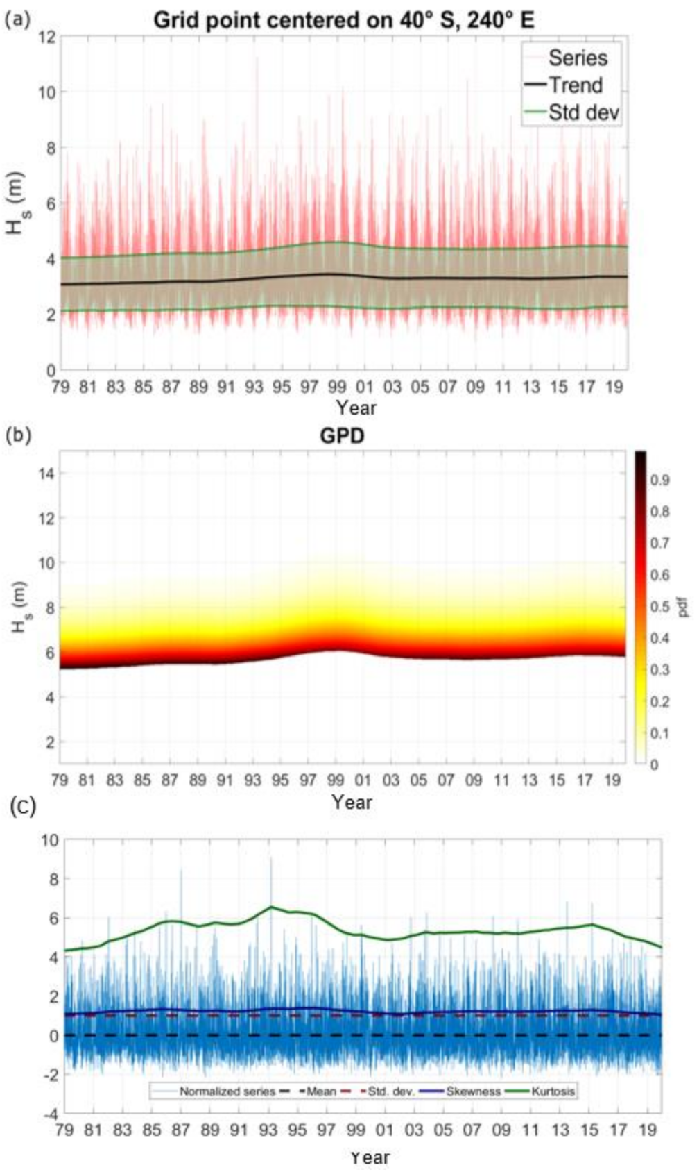
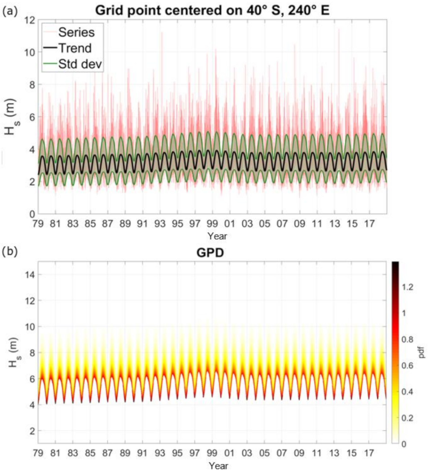
Figure 1 shows examples of the time series of $H_s$ (Figure 1a) and the resulting non-stationary non-seasonal GPD pdf as a function of time (1979–2019) (Figure 1b) for the location 40° S, 240° E. This is a location in the Pacific basin of the Southern Ocean, west of South America. This location was selected as an example of a point where the subsequent analysis shows there is a statistically significant trend in the extreme wave height. As evident in Figure 1a, there is a positive (increase) trend in the mean values over this period. The resulting non-stationary pdf is shown in Figure 1b over this period. In addition, there is also a clear positive trend in the pdf. Both the time series and the pdf show that the trend is not linear over this period, with clear variations with time. These long-duration variations in the trend may be associated with multi-decadal climate variability, such as El Nino [39] or with the impact of the advent of satellite data assimilation, which occurred around 1990 [40]. Figure 1c shows the transformed (stationary) time series. As can be seen, the transformed time series has a constant mean of zero and a constant variance (standard deviation) of one. The kurtosis and skewness, as a function of time, are also shown. These higher-order statistics are reasonably constant, indicating the transformed time series is approximately stationary. The results shown in Figure 1c are typical of most regions of the globe, indicating the suitability of the transformation used.

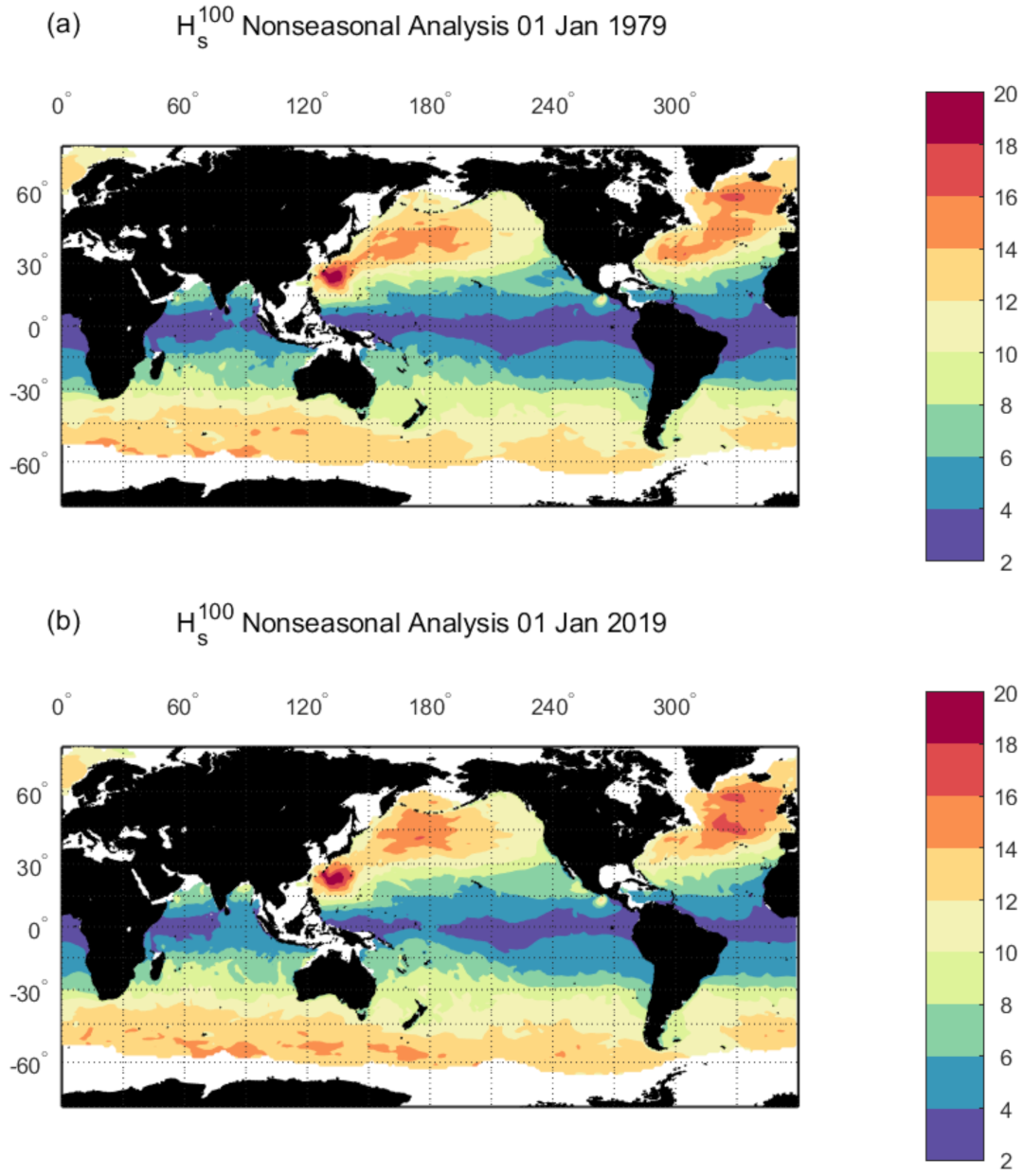
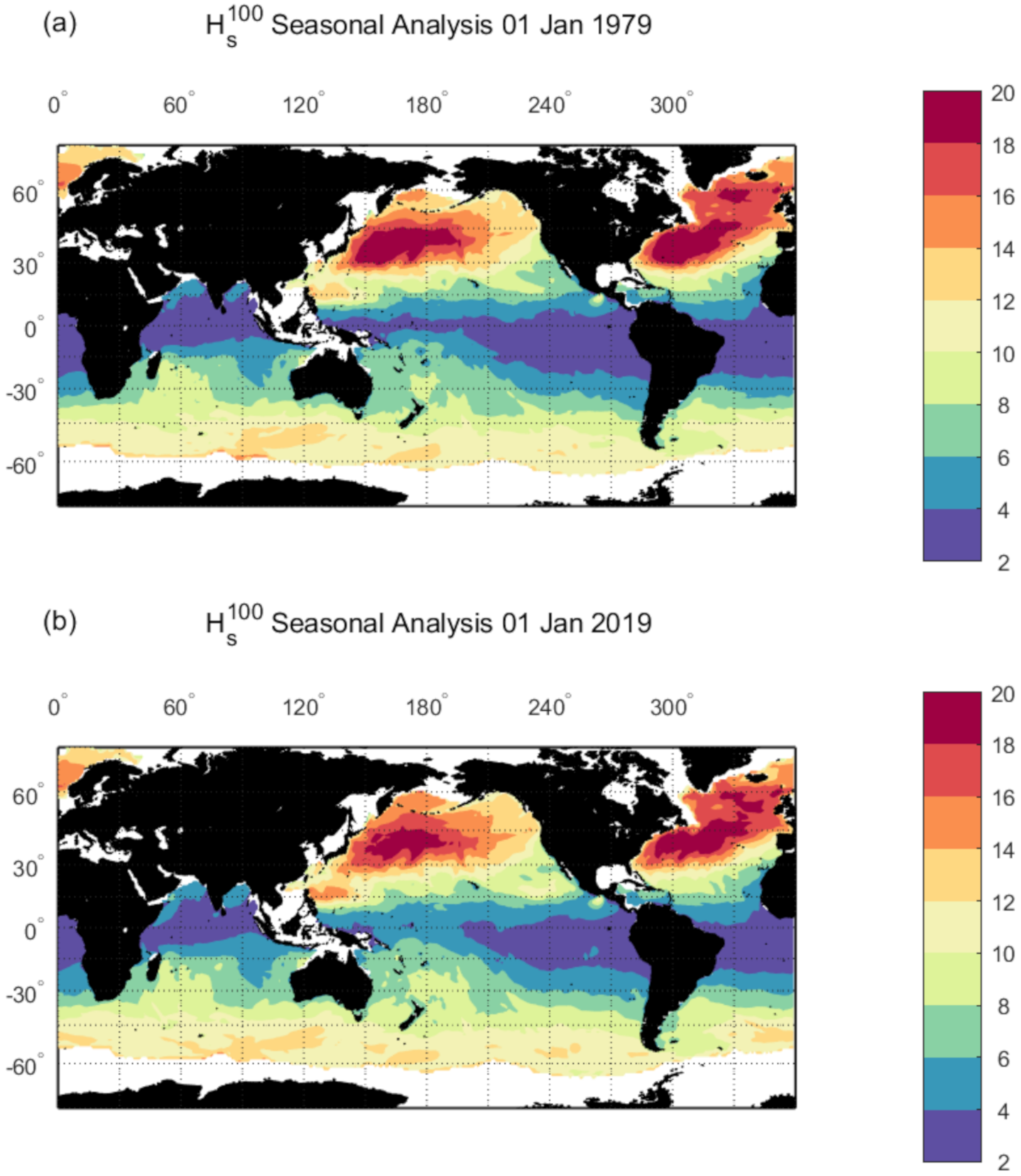
This non-seasonal analysis was applied at five-year intervals from 1 January 1979 to 1 January 2019, with $H_s^{100}$ determined at each point on the global grid. Figure 2 shows the resulting colour-filled contours of non-seasonal $H_s^{100}$ for 1 January 1979 (Figure 2a) and 1 January 2019 (Figure 2b). The results are generally consistent with previous analyses using conventional EVA approaches obtained from both satellite and model datasets [12,13,14,21]. The results show the largest values of $H_s^{100}$ in the North Atlantic and North Pacific with these values displaced towards the western boundaries of both of these oceanic basins. This corresponds to the storm tracks for both basins [21]. Values of $H_s^{100}$ across the Southern Ocean are quite consistent but slightly lower than values at the same latitudes in the Northern Hemisphere. The region of intense and frequent typhoons is evident in the western North Pacific. The zonal variation in extreme values is also apparent with the equatorial values being much smaller than at higher latitudes.

Note that as ERA5 is a deepwater global dataset, it has limited validity in coastal waters where finite depth and coastal details need to be defined at a resolution higher than the 0.5° resolution of the reanalysis. In addition, the TS EVA approach often could not fit a reasonable GPD approximation to the pdf in such regions. As a result, these coastal locations are not shaded in Figure 2 and subsequent plots. In addition, regions covered by ice for part of the year are also shaded white.

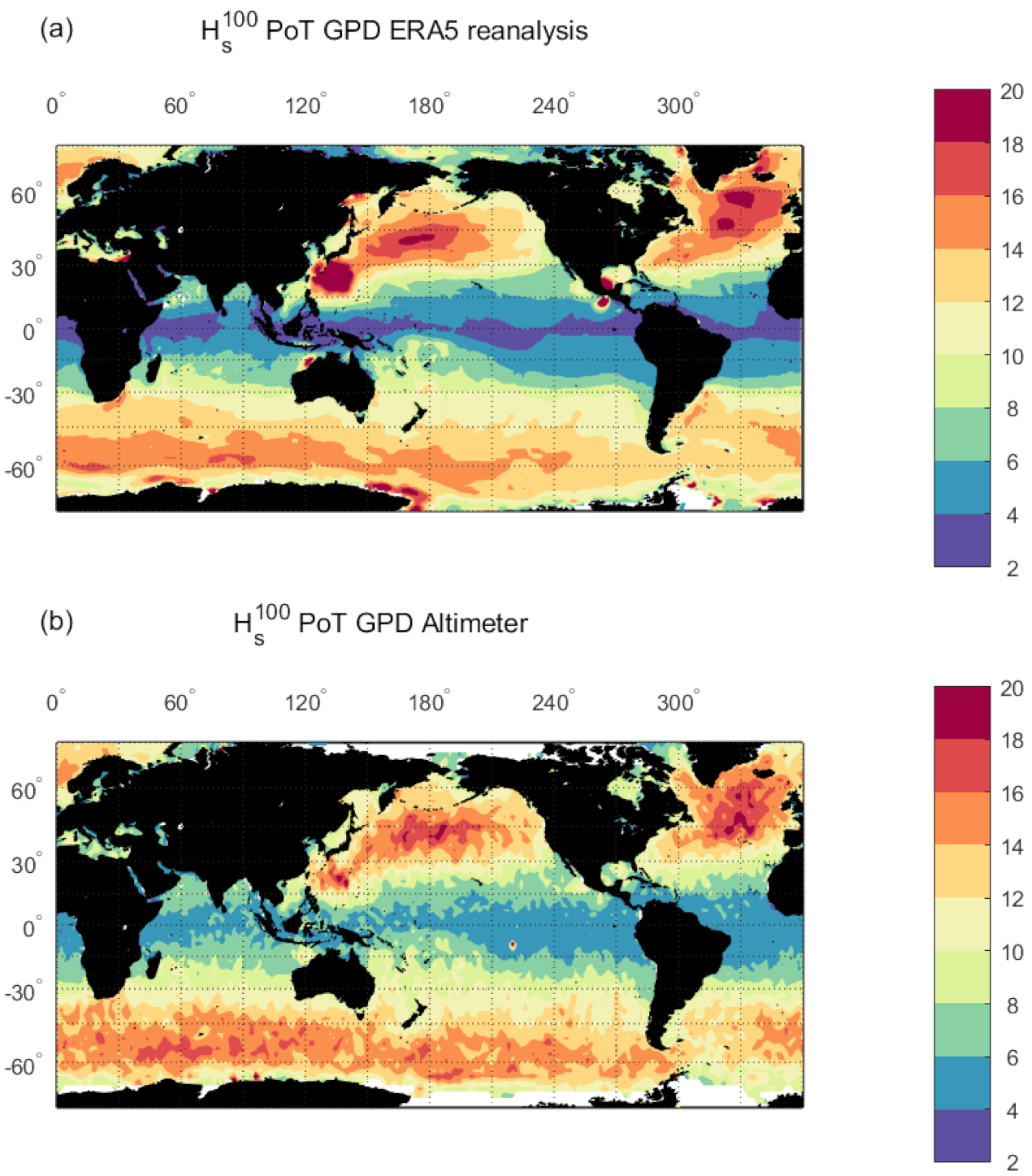
Figure 3 shows a comparison with the results of a conventional PoT GPD analysis (i.e., assumes the data are stationary) applied to both the present ERA5 data (Figure 3a) and altimeter data (Figure 3b), as in Takbash et al. [21]. The ERA5 results (Figure 3a) were obtained with a threshold set at the 70th percentile (as in Figure 2). The altimeter results use a 90th percentile threshold [21]. The ERA5 results are in good global agreement with the altimeter results. The ERA5 values are slightly smaller in magnitude than the altimeter results, consistent with previous studies [6,13,14], which show that models tend to slightly underestimate extreme wave height. The spatial distributions of extremes for the ERA5 conventional EVA analysis (Figure 3a) and the TS analysis (Figure 2) are, however, in good agreement with the altimeter results. It should also be noted that the threshold value chosen in the present analysis (70th percentile) differs from that of Takbash et al. [21] (90th percentile). A range of values for the threshold was tested for the present analysis. For most regions of the globe, the resulting values of $H_s^{100}$ were not significantly affected by the choice of the threshold value. In the typhoon region of the western North Pacific, however, a threshold value greater than the 70th percentile resulted in unreasonably large values. Examination of the pdfs for this region showed that this was because a higher threshold resulted in too few values in the pdf to adequately define the tail of the distribution. It is believed this is because of the relatively infrequent occurrence of typhoons and the likelihood that the model resolution is such that many such storms are not adequately resolved [13]. Therefore, although we acknowledge the choice of a 70th percentile threshold is relatively low, we believe it is a reasonable compromise for such a global analysis and does not significantly bias the results. Certainly, these results are consistent with calculations with higher percentile thresholds and with the comparisons with altimeter $H_s^{100}$ (Figure 3).

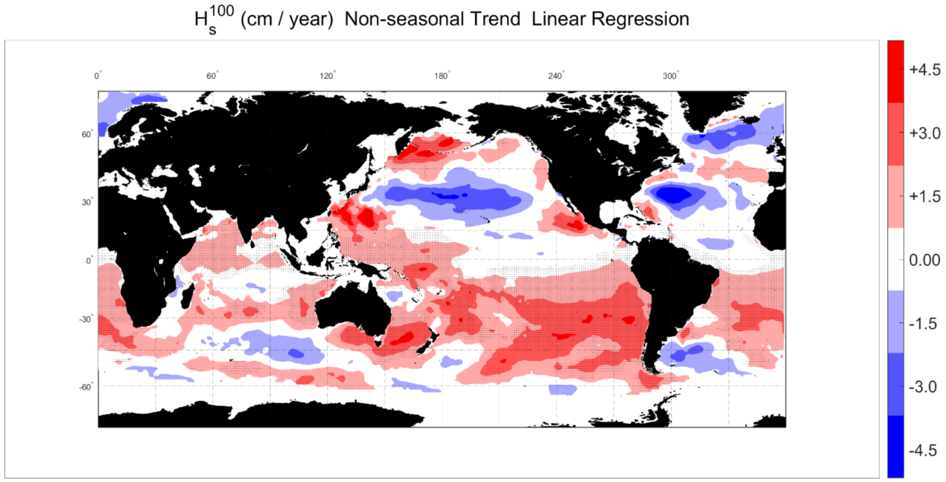
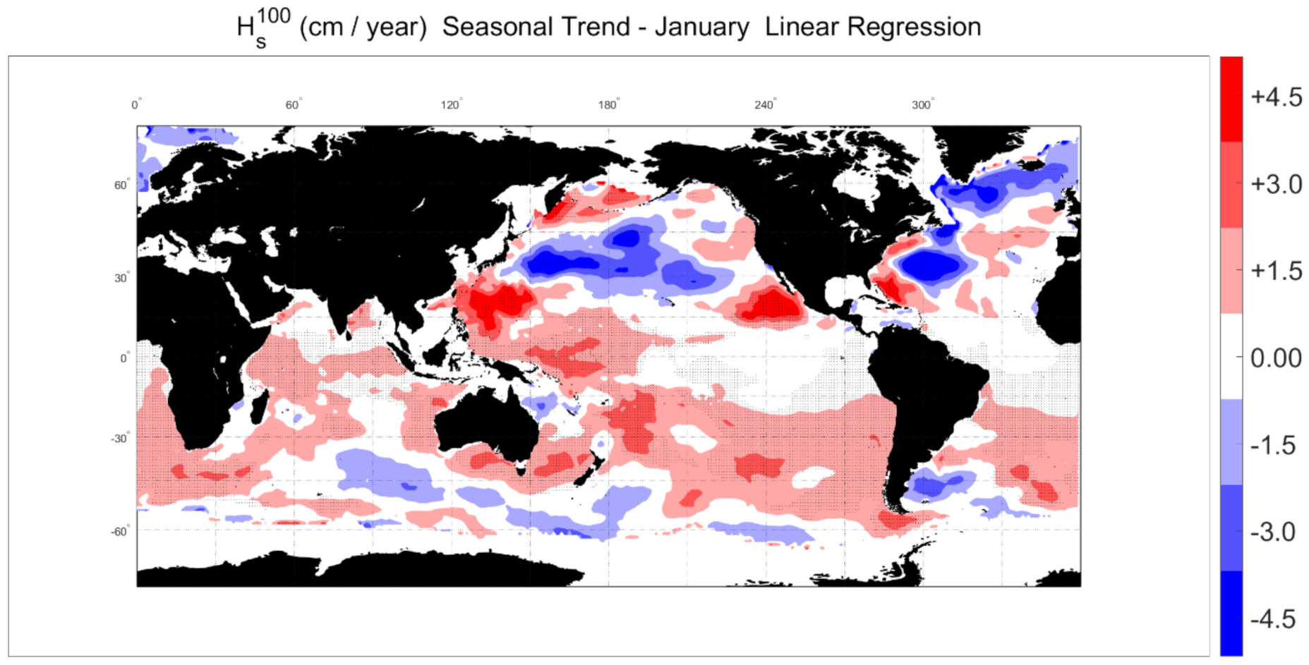
Comparison of the values of $H_s^{100}$ between 1979 (Figure 2a) and 2019 (Figure 2b) show regions where there are apparent differences. The comparison suggests increased values of $H_s^{100}$ in the Southern Ocean and South Pacific in more recent years. There is also an increase in the typhoon regions of the western North Pacific and the hurricane regions off the west coast of the United States. Such changes are more clearly shown in Figure 4, which shows the linear trend over the period 1979–2019. In addition, regions for which the trend is statistically significant at the 95% level (based on the p-value) are shown with shading, as a measure of the statistical confidence of the trend.

Figure 4 confirms the results seen in Figure 3 that there is a generally positive trend across significant regions of the Southern Hemisphere (greater than 15° S), in the typhoon belt of the western North Pacific and the hurricane regions off the west coast of the United States. There are also increases (statistically significant) in the high latitudes of the North Pacific (greater than 50° N). In the Atlantic, positive trends occur in the hurricane regions to the east of the United States and the South Atlantic (extratropical cyclones region [41]). There are also negative trends in the trade wind belts of the North Pacific and North Atlantic ($\sim 30°$ N). However, for these regions the trend is not statistically significant. As a result, there is less statistical confidence in these negative trends.

The spatial distributions of positive trends shown in Figure 4 are generally consistent with the results of the altimeter data of Young et al. [9], which were obtained with a “stationary slice” approach and an IDM analysis. Published 90th percentile $H_s$ trends for altimeter data [7,8] also show increases in the Southern Hemisphere, although these tend to be further south in the Southern Ocean than the present EVA results. In addition, the results in Figure 4 indicate that the largest values of the positive trend in the Southern Hemisphere occur in the Pacific basin of the Southern Ocean. In contrast, previous results for mean and upper percentile trends suggested the largest values were in the Indian Ocean basin of the Southern Ocean [7,8]. The present analysis indicates the largest values of the trend are approximately +3 cm/yr, indicating an increase of approximately 1.2 m over the 41 year period of the record, consistent with the differences shown in Figure 2.

4.2. Seasonal Analysis—January

Figure 5 shows an example of the resulting time series and pdf for the non-stationary seasonal GPD analysis as a function of time for the location 40°S, 240°E (as in Figure 1). Compared to Figure 1, the seasonal variation is now evident, with larger waves in winter (July) than in summer (January). The seasonal analysis enables an understanding of whether the extreme conditions are dominated by a particular season or whether there is a more consistent year-round contribution of extremes. For the seasonal analysis, values of $H_s^{100}$ are determined by season (month) and year. As a result, trends can then be determined for each season. Therefore, for example, $H_s^{100}$ can be determined for January of each year and the trend evaluated across these values. As with the non-seasonal analysis, such values were determined at 5-year intervals and the trend determined using linear regression.

Figure 6 shows the values of $H_s^{100}$ on a seasonal basis for January 1979 (Figure 6a) and January 2019 (Figure 6b). January corresponds to the Northern Hemisphere winter and hence, as expected, extreme values in the high latitudes of the North Pacific and North Atlantic are slightly higher than the nonseasonal result (Figure 2) ($\sim 22$ m compared to $\sim 18$ m). This occurs because the Northern Hemisphere has a significant seasonal cycle (winter to summer), with most storms occurring during winter. In contrast, summer conditions in these northern latitudes are relatively calm [42]. Therefore, the probability of occurrence of extremes is increased in January compared to the full year and hence the values of $H_s^{100}$ are larger for the seasonal analysis. In contrast, extreme values for the Southern Ocean for January are smaller than for the non-seasonal analysis (Figure 2) ($\sim 12$ m compared to $\sim 14$ m), as this is now the Southern Hemisphere summer. The difference is not as large as for the Northern Hemisphere winter, as the seasonal variation in wave conditions in the Southern Hemisphere is less than that for the Northern Hemisphere. That is, the Southern Ocean is relatively rough year-round [42,43].

It is also clear in Figure 6 that the extremes associated with western Pacific typhoons and United States hurricanes are significantly reduced, as these tropical low-pressure systems do not occur at this time of year.

The trends in values of $H_s^{100}$ for January are shown in Figure 7. The spatial distributions of the trends are similar to the non-seasonal result (Figure 4). However, the magnitude of the increase in the Southern Hemisphere for the seasonal result for January is much smaller than for the non-seasonal case. This suggested that the increases in $H_s^{100}$ in these regions are associated with a strengthening in Southern Hemisphere storms during winter. As noted above and shown in Figure 6, values of extreme wave height associated with typhoons in the western North Pacific and hurricanes off the west coast of North America are not large during January. However, it is evident in Figure 7 (and also Figure 6) that $H_s^{100}$ in both of these regions has increased over the 41-year period. This suggests that both typhoons and hurricanes in these basins may be occurring more frequently in these winter periods in recent years.

4.3. Seasonal Analysis—July

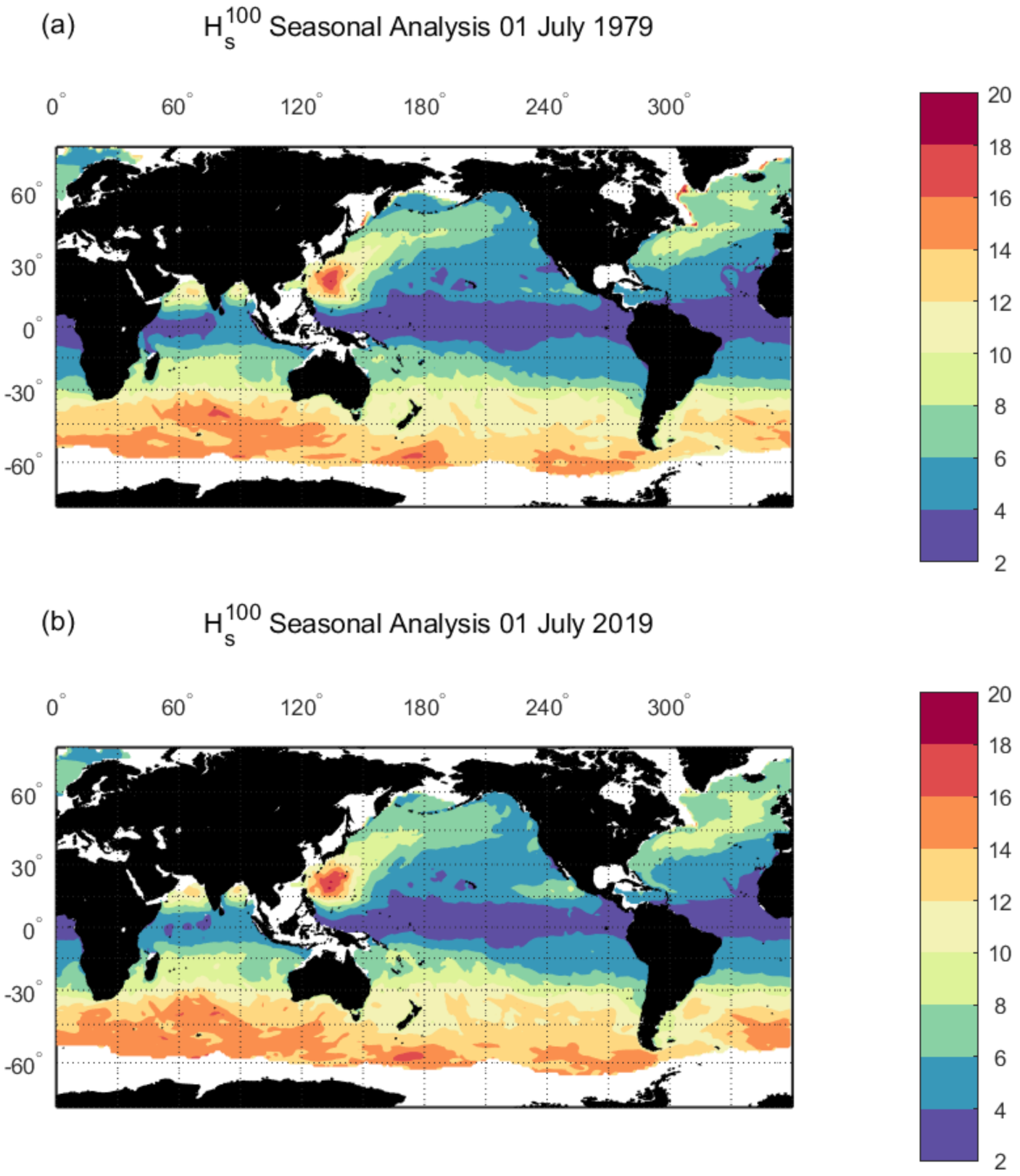
Figure 8 shows the values of $H_s^{100}$ from the seasonal analysis for July for 1979 (Figure 8a) and July 2019 (Figure 8b). Consistent with Figure 6, the maximum values of $H_s^{100}$ in the Southern Hemisphere (winter) are slightly higher than the corresponding non-seasonal case (Figure 2). For the high-latitude regions of the North Pacific and North Atlantic, the maximum values of $H_s^{100}$ are, however, much smaller than for the non-seasonal case ($\sim 6$ m compared to $\sim 18$ m). This again demonstrates that the Northern Hemisphere has a significant seasonal cycle, with summer conditions (July) relatively calm [43]. As a result, the July values of $H_s^{100}$ are much smaller than the non-seasonal analysis (Figure 2) and the winter (January) conditions (Figure 6). The large values of $H_s^{100}$ associated with typhoons in the western North Pacific are now clearly evident in the analysis for July, reflecting the time of year when these tropical systems occur.

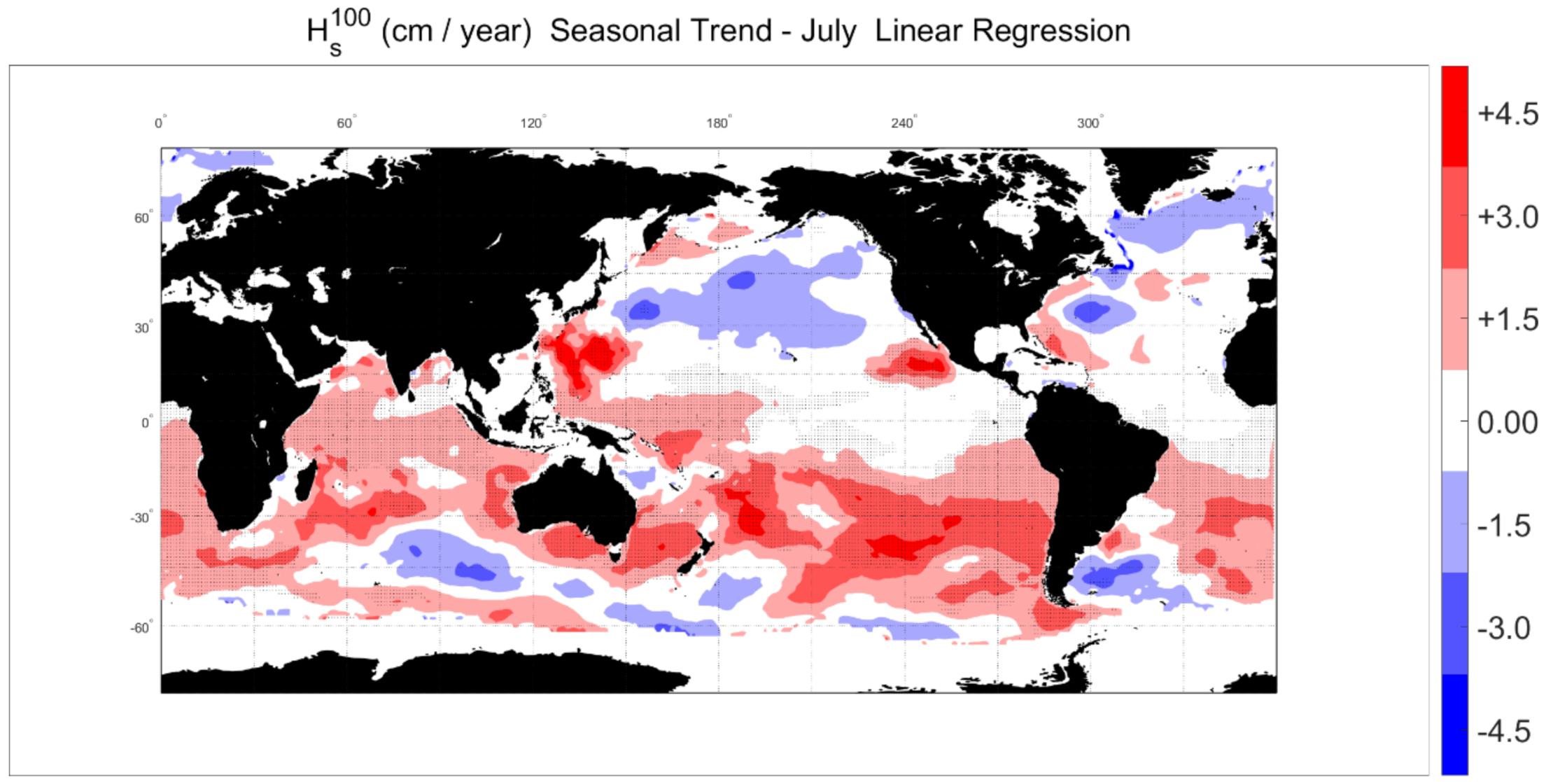
The trend for $H_s^{100}$ in July is shown in Figure 9. The spatial trends are similar to the seasonal trend for January (Figure 7) and the non-seasonal case (Figure 4). Compared to the trend for January there are, however, clear differences in the magnitude of the trends. During July, the trends in the Southern Ocean are more strongly positive than in January. Again, this indicates that the increasing trend for $H_s^{100}$ in the Southern Ocean appears to be associated with strengthening extreme waves during winter. Similarly, the negative trend in the North Pacific and North Atlantic is more strongly negative than for January. This result, however, needs to be treated with caution as these trends are not statistically significant.

5. Discussion

The present results indicate that the 100-year return period significant wave height, $H_s^{100}$, as modelled by the ERA5 reanalysis dataset has increased at a rate up to +3 cm/year in the Southern Hemisphere over the 41-year period from 1979 to 2019. As values of $H_s^{100}$ in the Southern Ocean are typically approximately 15 m, this equates to a percentage increase of 0.2% per year or 8% over the 41-year period. The present result represents the first attempt to determine changes in extreme wave heights over the past decades using a robust extreme value approach. It is interesting to compare these results with previous studies.

Young et al. [9] analyzed a 16-year altimeter dataset (1992-2008) to estimate $H_s^{100}$. The analysis had the limitations that the period was relatively short and was analyzed using a “time slice” method and an IDM approach to the extreme value analysis. Despite this, the spatial distributions of $H_s^{100}$ are remarkably similar to the present results, showing positive trends over the Southern Hemisphere and weaker negative trends for the Northern Hemisphere. For the Southern Hemisphere, the magnitude of the trend was approximately +4 cm/year, comparable to +3 cm/year in the present study.

Young and Ribal [8] re-examined altimeter data but over a more extensive 33-year period from 1985 to 2018. They examined trends in the mean and 90th percentile $H_s$, finding weak positive trends in mean conditions and larger trends for the 90th percentile. Again, the 90th percentile values showed positive trends in the Southern Hemisphere and weaker negative trends in the Northern Hemisphere. Their positive trends in the Southern Hemisphere were approximately +1 cm/year. As their results seem to indicate that extremes were increasing faster than mean conditions, one would expect the 90th percentile result to be smaller than $H_s^{100}$. Although a 90th percentile cannot be directly compared to $H_s^{100}$, the Young and Ribal [8] result is consistent with the present result.

Morim et al. [5] and Meucci et al. [10] considered future projections of wave climate using an ensemble of model results for a range of atmospheric emission scenarios. They projected positive trends in the wave climate in the Southern Hemisphere and smaller negative trends in the Northern Hemisphere. Morim et al. [5] projected increases of the 99th percentile $H_s$ of 5% to 10% between the present day and 2100 (an increase of approximately +2 cm/year). Meucci et al. [10] also projected increases of $H_s^{100}$ in the Southern Ocean of 5% to 10% over this period (approximately +2.5 cm/year).

Hence, all of these findings are consistent with the present results. The reliability of the present result does, however, depend on whether reanalysis models can reproduce trends in extreme values. Here, there are potentially two limitations, firstly, whether models can accurately reproduce extreme values. A number of studies have compared reanalysis model estimates of $H_s^{100}$ with both buoy and altimeter data [12,13,14], showing that model results may be 10% lower than buoy and altimeter data. The spatial distributions of reanalysis data are, however, reproduced well. This is confirmed in Figure 3, where conventional (i.e., time series assumed stationary) EVA analyses of both the present ERA5 reanalysis data and altimeter observations show global values of $H_s^{100}$ with a similar magnitude and spatial distribution. The other issue which needs to be considered is whether the inclusion of altimeter assimilation in the ERA5 reanalysis dataset in approximately 1990 introduced a discontinuity in the dataset which significantly impacts trend estimates [4,40]. Timmermans et al. [2] compared trends in mean $H_s$ for ERA5 and the ECMWF CY46R1 (Cycle 46R1) product. CY46R1 is very similar to ERA5 but without altimeter data assimilation. Over the period 1992–2017, ERA5 and CY46R1 yielded very similar spatial distributions of the trend in mean $H_s$, with CY46R1 producing slightly higher values. Although this is a shorter period than the present analysis, it does add some confidence that the assimilation does not grossly distort the trend estimates of mean values. The behaviour at the extremes is still unclear.

6. Conclusions

The present study has undertaken a non-stationary TS extreme value analysis of a 41-year record of global ERA5 reanalysis data of significant wave height, $H_s$. The global distribution of values of the 100-year return period significant wave height, $H_s^{100}$, from the non-stationary analysis is consistent with previous results using conventional stationary approaches. The non-stationary analysis, however, allows the determination of changes in $H_s^{100}$ over the data period (1979–2019). This analysis shows that there have been statistically significant changes in $H_s^{100}$ over this period. In particular, there has been an increase in $H_s^{100}$ in the Southern Hemisphere of up to +3 cm/year. The Northern Hemisphere shows a smaller negative trend, although these values are generally not statistically significant. The seasonal analysis of the data shows that the positive trend in the Southern Hemisphere is a result of an increase in the intensity of winter storms or the frequency of these storms, or both.

Both the spatial distribution of changes in $H_s^{100}$ and the magnitudes are consistent with the previous limited analyses of global extreme wave height trends, both for the historical period and future projections. These various analyses show that there have been clear increases in $H_s^{100}$ over the past 41 years in the Southern Hemisphere and that this is projected to continue in the future.

References

- Gemmrich, J.; Thomas, B.; Bouchard, R. Observational changes and trends in northeast Pacific wave records. Geophys. Res. Lett. 2011, 38, L22601. [Google Scholar] [CrossRef]
- Timmermans, B.W.; Gommenginger, C.P.; Dodet, G.; Bidlot, J.-R. Global Wave Height Trends and Variability from New Multimission Satellite Altimeter Products, Reanalyses, and Wave Buoys. Geophys. Res. Lett. 2020, 47, e2019GL086880. [Google Scholar]
- Hemer, M.A. Historical trends in Southern Ocean storminess: Long-term variability of extreme wave heights at Cape Sorell, Tasmania. Geophys. Res. Lett. 2010, 37, L18601. [Google Scholar] [CrossRef]
- Aarnes, O.J.; Abdulla, S.; Bidlot, J.R.; Breivik, O. Marine wind and wave height trends at different ERA-Interim forecast ranges. J. Clim. 2015, 28, 819–837. [Google Scholar] [CrossRef] [Green Version]
- Morim, J.; Hemer, M.; Wang, X.L.; Cartwright, N.; Trenham, C.; Semedo, A.; Young, I.; Bricheno, L.; Camus, P.; Casas-Prat, M.; et al. Robustness and uncertainties in global multivariate wind-wave climate projections. Nat. Clim. Chang. 2019, 9, 711–718. [Google Scholar] [CrossRef] [Green Version]
- Stopa, J.E.; Cheung, K.F. Intercomparison of wind and wave data from the ECMWF Reanalysis Interim and the NCEP Climate Forecast System Reanalysis. Ocean. Model. 2014, 75, 65–83. [Google Scholar] [CrossRef]
- Young, I.R.; Zieger, S.; Babanin, A.V. Global trends in wind speed and wave height. Science 2011, 332, 451–455. [Google Scholar] [CrossRef]
- Young, I.R.; Ribal, A. Multi-platform evaluation of global trends in wind speed and wave height. Science 2019, 364, 548–552. [Google Scholar] [CrossRef]
- Young, I.R.; Vinoth, J.; Zieger, S.; Babanin, A.V. Investigation of trends in extreme wave height and wind speed. J. Geophys. Res. 2012, 117, C00J06. [Google Scholar] [CrossRef]
- Meucci, A.; Young, I.R.; Hemer, M.K.E.; Ranasinghe, R. Projected 21st century changes in extreme wind-wave events. Sci. Adv. 2020, 6, eaaz7295. [Google Scholar] [CrossRef]
- Vinoth, J.; Young, I.R. Global Estimates of Extreme Wind Speed and Wave Height. J. Clim. 2011, 24, 1647–1665. [Google Scholar] [CrossRef]
- Breivik, O.; Aarnes, O.J.; Abdalla, S.; Bidlot, J.R.; Janssen, P.A. Wind and wave extremes over the world oceans from very large ensembles. Geophys. Res. Lett. 2014, 41, 5122–5131. [Google Scholar] [CrossRef] [Green Version]
- Meucci, A.; Young, I.R.; Breivik, O. Wind and wave extremes from atmosphere and wave model ensembles. J. Clim. 2018, 31, 8819–8893. [Google Scholar] [CrossRef]
- Takbash, A.; Young, I.R. Global ocean extreme wave heights from spatial ensemble data. J. Clim. 2019, 32, 6823–6836. [Google Scholar] [CrossRef]
- Mentaschi, L.; Vousdoukas, M.; Vououvalas, E.; Sartini, L.; Feyen, L.; Besio, G.; Alfieri, L. The transformed-stationary approach: A generic and simplified methodology for non-stationary extreme value analysis. Hydrol. Earth Sys. Sci. 2016, 20, 3527–3547. [Google Scholar] [CrossRef] [Green Version]
- Hersbach, H.; Bell, B.; Berrisford, P.; Hirahara, S.; Horanyi, A.; Munoz-Sabater, J.; Nicolas, J.; Peubey, C.; Radu, R.; Schepers, D.; et al. The ERA5 global reanalysis. Q. J. R. Meteorol. Soc. 2020, 146, 1999–2049. [Google Scholar] [CrossRef]
- Goda, Y. Uncertainty in design parameter from the viewpoint of statistical variability. J. Offshore Mech. Arct. Eng. 1992, 114, 76–82. [Google Scholar] [CrossRef]
- Coles, S. An Introduction to Statistical Modelling of Extremes, 1st ed.; Springer London Ltd.: London, UK, 2001; p. 209. [Google Scholar]
- Tucker, M.J. Waves and Ocean. Engineering, 1st ed.; Ellis Horwood: Chichester, NY, USA, 1991; p. 431. [Google Scholar]
- Alves, J.H.G.M.; Young, I.R. On estimating extreme wave heights using combined Geosat, Topex/Poseidon and ERS-1 altimeter data. Appl. Ocean. Res. 2003, 25, 167–186. [Google Scholar] [CrossRef]
- Takbash, A.; Young, I.R.; Breivik, O. Global wind speed and wave height extremes derived from satellite records. J. Clim. 2019, 32, 109–126. [Google Scholar] [CrossRef]
- Castillo, E. Extreme Value Theory in Engineering, 1st ed.; Academic Press: New York, NY, USA, 1988; p. 389. [Google Scholar]
- Cheng, L.; AghaKouchak, A.; Gilleland, E.; Katz, R.W. Nonstationary extreme value analysis in a changing climate. Clim. Chang. 2014, 127, 353–369. [Google Scholar] [CrossRef]
- Menéndez, M.; Méndez, F.J.; Izaguirre, C.; Luceño, A.; Losada, I.J. The influence of seasonality on estimating return values of significant wave height. Coast. Eng. 2009, 56, 211–219. [Google Scholar] [CrossRef]
- Méndez, F.J.; Menéndez, M.; Luceño, A.; Losada, I.J. Estimation of the long-term variability of extreme significant wave height using a time-dependent peak over threshold (pot) model. J. Geophys. Res. Ocean. 2006, 111, C07024. [Google Scholar] [CrossRef]
- Méndez, F.J.; Menéndez, M.; Luceño, A.; Medina, R.; Graham, N.E. Seasonality and duration in extreme value distributions of significant wave height. Ocean. Eng. 2008, 35, 131–138. [Google Scholar] [CrossRef]
- Hundecha, Y.; St-Hilaire, A.; Ouarda, T.B.M.J.; El Adlouni, S.; Gachon, P. A nonstationary extreme value analysis for the assessment of changes in extreme annual wind speed over the Gulf of St. Lawrence, Canada. J. App. Met. Clim. 2008, 47, 2745–2759. [Google Scholar] [CrossRef]
- Renard, B.; Sun, X.; Lang, M. Bayesian methods for non-stationary extreme value analysis. In Extremes in a Changing Climate, 1st ed.; AghaKouchak, A., Easterling, D., Hsu, K., Schubert, S., Sorooshian, S., Eds.; Springer Netherlands: Dordrecht, The Netherlands, 2013; pp. 39–95. [Google Scholar]
- Bender, J.; Wahl, T.; Jensen, J. Multivariate design in the presence of non-stationarity. J. Hydrol. 2014, 514, 123–130. [Google Scholar] [CrossRef]
- Galiatsatou, P.; Makris, C.; Prinos, P.; Kokkinos, D. Nonstationary joint probability analysis of extreme marine variables to assess design water levels at the shoreline in a changing climate. Nat. Hazards 2019, 98, 1051–1089. [Google Scholar] [CrossRef]
- Leonard, M.; Westra, S.; Phatak, A.; Lambert, M.; van den Hurk, B.; McInnes, K.; Risbey, J.; Schuster, S.; Jakob, D.; Stafford-Smith, M. A compound event framework for understanding extreme impacts. Wiley Interdiscip. Rev. Clim. Chang. 2014, 5, 113–128. [Google Scholar] [CrossRef]
- Mazas, F.; Hamm, L. An event-based approach for extreme joint probabilities of waves and sea levels. Coast. Eng. 2017, 122, 44–59. [Google Scholar] [CrossRef]
- Zscheischler, J.; Westra, S.; Van Den Hurk, B.J.; Seneviratne, S.I.; Ward, P.J.; Pitman, A.; AghaKouchak, A.; Bresch, D.N.; Leonard, M.; Wahl, T.; et al. Future climate risk from compound events. Nat. Clim. Chang. 2018, 8, 469–477. [Google Scholar] [CrossRef]
- Vousdoukas, M.I.; Voukouvalas, E.; Menttaschi, L.; Dottori, F.; Giardino, A.; Bouziotas, D.; Bianchi, A.; Salamon, P.; Feyen, L. Developments in large-scale coastal flood hazard mapping. Nat. Hazards Earth Syst. Sci. 2016, 16, 1841–1853. [Google Scholar] [CrossRef] [Green Version]
- Hasselmann, K.; Bauer, E.; Janssen, P.A.E.M.; Komen, G.J.; Bertotti, L.; Lionello, P.; Guillaume, A.; Cardone, V.C.; Greenwood, J.A.; Reistad, M.; et al. The WAM model-A third generation ocean wave prediction model. J. Phys. Oceanogr. 1988, 18, 1775–1810. [Google Scholar]
- Lionello, P.; Gunther, H.; Janssen, P.A.E.M. Assimilation of altimeter data in a global Third-generation wave model. J. Geophys. Res. 1992, 97, 14453–14474. [Google Scholar] [CrossRef]
- Mann, H.B. Nonparametric Tests against Trend. Econometrica 1945, 13, 245–259. [Google Scholar] [CrossRef]
- Sen, P.K. Estimates of the regression coefficient based on Kendall’s TAU. Am. Stats. Assoc. J. 1968, 63, 1379–1389. [Google Scholar] [CrossRef]
- Stopa, J.E.; Cheung, K.F.; Tolman, H.L.; Chawla, A. Patters and cycles in the Climate Forecast System Reanalysis wind and wave data. Ocean Model. 2013, 70, 207–220. [Google Scholar] [CrossRef]
- Meucci, A.; Young, I.R.; Aarnes, O.J.; Breivik, O. Comparison of Wind Speed and Wave Height Trends from Twentieth-Century Models and Satellite Altimeters. J. Clim. 2020, 33, 611–624. [Google Scholar] [CrossRef]
- Mendes, D.; Souza, E.P.; Marengo, J.A.; Mendes, M.C. Climatology of extratropical cyclones over the South American-southern oceans sector. Theor. Appl. Climatol. 2010, 100, 239–250. [Google Scholar] [CrossRef] [Green Version]
- Young, I.R.; Donelan, M.A. On the determination of global ocean wind and wave climate from satellite observations. Remote Sens. Environ. 2018, 215, 228–241. [Google Scholar] [CrossRef]
- Young, I.R. Seasonal variability of the global ocean wind and wave climate. Int. J. Clim. 1999, 19, 931–950. [Google Scholar] [CrossRef]
Figure 1.
The non-stationary TS analysis for a location at 40° S, 240° E. (a) The time series of (m) as a function of time (1979–2019) with the mean and standard deviation marked. (b) The GPD pdf as a function of time. (c) Transformed time series with constant mean and standard deviation. The skewness and kurtosis are approximately constant, indicating stationarity.
Figure 2.
Global long-term (time-dependent) values of (m) obtained with the non-stationary PoT analysis and a GPD distribution using the non-seasonal TS method (a) 1 January 1979 and (b) 1 January 2019. Data obtained from ERA-5 reanalysis 1979–2019. White regions represent coastal locations where the TS EVA did not produce acceptable fits to the pdf or regions covered by sea ice.
Figure 3.
Global distribution of (m) from conventional PoT GPD analyses (i.e., data assumed stationary over time). (a) Analysis using the ERA5 dataset used in the remainder of this paper. (b) Altimeter data, as in Takbash et al. [21].
Figure 4.
Global non-seasonal long-term trend (cm/yr) of over the period 1979–2019 from the non-stationary TS EVA approach with a GPD. Values which are statistically significant are shown with shaded dots.
Figure 5.
The non-stationary seasonal TS analysis for a location at 40° S, 240° E. (a) The time series of (m) as a function of time (1979–2019) with the mean and standard deviation marked. (b) The GPD pdf as a function of time. The seasonal cycle is evident in both panels.
Figure 6.
Global long-term (time-dependent) values of (m) obtained with a PoT analysis and a GPD distribution using the seasonal TS method (a) 1 January 1979 and (b) 1 January 2019. Data obtained from ERA-5 reanalysis 1979–2019. White regions represent coastal locations where the TS EVA did not produce acceptable fits to the pdf or regions covered by sea ice.
Figure 7.
Global seasonal long-term trend (cm/yr) of for January over the period 1979–2019 from the non-stationary seasonal TS EVA approach with a GPD. Values which are statistically significant are shown with shaded dots.
Figure 8.
Global long-term (time-dependent) values of (m) obtained with a PoT analysis and a GPD distribution using the seasonal TS method (a) 1 July 1979 and (b) 1 July 2019. Data obtained from ERA-5 reanalysis 1979–2019. White regions represent coastal locations where the TS EVA did not produce acceptable fits to the pdf or regions covered by sea ice.
Figure 9.
Global seasonal long-term trend (cm/yr) of for July over the period 1979–2019 from the non-stationary seasonal TS EVA approach with a GPD. Values which are statistically significant are shown with shaded dots.
Publisher’s Note: MDPI stays neutral with regard to jurisdictional claims in published maps and institutional affiliations. |
© 2020 by the authors. Licensee MDPI, Basel, Switzerland. This article is an open access article distributed under the terms and conditions of the Creative Commons Attribution (CC BY) license (http://creativecommons.org/licenses/by/4.0/).
Share and Cite
MDPI and ACS Style
Takbash, A.; Young, I.R. Long-Term and Seasonal Trends in Global Wave Height Extremes Derived from ERA-5 Reanalysis Data. J. Mar. Sci. Eng. 2020, 8, 1015. https://doi.org/10.3390/jmse8121015
AMA Style
Takbash A, Young IR. Long-Term and Seasonal Trends in Global Wave Height Extremes Derived from ERA-5 Reanalysis Data. Journal of Marine Science and Engineering. 2020; 8(12):1015. https://doi.org/10.3390/jmse8121015
Chicago/Turabian StyleTakbash, Alicia, and Ian R. Young. 2020. "Long-Term and Seasonal Trends in Global Wave Height Extremes Derived from ERA-5 Reanalysis Data" Journal of Marine Science and Engineering 8, no. 12: 1015. https://doi.org/10.3390/jmse8121015
Note that from the first issue of 2016, this journal uses article numbers instead of page numbers. See further details here.