Article

Effects of Wave-Induced Sea Ice Break-Up and Mixing in a High-Resolution Coupled Ice-Ocean Model

1
Department of Infrastructure Engineering, University of Melbourne, Melbourne, VIC 3010, Australia
2
Laboratory for Regional Oceanography and Numerical Modeling, Qingdao National Laboratory for Marine Science and Technology, Qingdao 266237, China
3
Australian Antarctica Division and Australian Antarctic Programme Partnership, University of Tasmania, Hobart, TAS 7001, Australia
4
Environmental Science and Engineering, University of Northern British Columbia, Prince George, BC V2N 4Z9, Canada
*
Author to whom correspondence should be addressed.
J. Mar. Sci. Eng. 2021, 9(4), 365; https://doi.org/10.3390/jmse9040365
Submission received: 9 March 2021 / Revised: 25 March 2021 / Accepted: 26 March 2021 / Published: 29 March 2021
(This article belongs to the Special Issue The Ice-Ocean Boundary)

Abstract

:
Arctic sea ice plays a vital role in modulating the global climate. In the most recent decades, the rapid decline of the Arctic summer sea ice cover has exposed increasing areas of ice-free ocean, with sufficient fetch for waves to develop. This has highlighted the complex and not well-understood nature of wave-ice interactions, requiring modeling effort. Here, we introduce two independent parameterizations in a high-resolution coupled ice-ocean model to investigate the effects of wave-induced sea ice break-up (through albedo change) and mixing on the Arctic sea ice simulation. Our results show that wave-induced sea ice break-up leads to increases in sea ice concentration and thickness in the Bering Sea, the Baffin Sea and the Barents Sea during the ice growth season, but accelerates the sea ice melt in the Chukchi Sea and the East Siberian Sea in summer. Further, wave-induced mixing can decelerate the sea ice formation in winter and the sea ice melt in summer by exchanging the heat fluxes between the surface and subsurface layer. As our baseline model underestimates sea ice cover in winter and produces more sea ice in summer, wave-induced sea ice break-up plays a positive role in improving the sea ice simulation. This study provides two independent parameterizations to directly include the wave effects into the sea ice models, with important implications for the future sea ice model development.

1. Introduction

Sea ice is crucial for modulating the global climate, not only because the sea ice cover reflects incoming solar radiation, but also because it creates an insulating layer between the ocean and the atmosphere. Therefore, the area occupied by sea ice moderates the energy transfer between the ocean and atmosphere through the positive sea ice-albedo feedback mechanism: the enlarged open water with small albedo will absorb more solar radiation, therefore heating the surface water and further accelerating the ice melting [1]. A rapid decline of sea ice extent tends to result in larger waves, in turn, providing energy to break up sea ice and further accelerate sea ice retreat [2]. Global warming has increased the wave activities in the Arctic, and bigger ocean waves affect sea ice formation and melting in the marginal ice zone (MIZ) [3]. Ocean waves will assist the ice-albedo feedback, therefore, the absence of wave-ice interactions parameterization will lead to the disagreement between the contemporary Earth system models and observations. Furthermore, the decrease of sea ice cover due to global warming affects Arctic shipping and engineering, such as transforming the Arctic into a navigable ocean with broken small floating ice floes [4] and ice-water-structure interaction [5]. Under this condition, wave-ice interactions become an important and challenging topic that needs to be considered in sea ice models to improve the performance of sea ice simulations.
In the MIZ, the ice cover will reduce the amplitude of ocean waves due to the processes of scattering and dissipation. Numerical models have been widely used to study wave scattering and attenuation in the MIZ. Bennetts et al. [6] constructed a three-dimensional model of ocean-wave scattering and found that wave attenuation highly depends on wave period and the average ice thickness, and linearly related to the sea ice concentration [7]. Furthermore, Bennetts compared the transmitted energies between theoretical models and experimental data and found that wave-energy attenuation is induced by an accumulation of scattering events [8]. Montiel et al. [9] proposed a linear three-dimensional model of wave attenuation in the MIZ based on potential flow theory and reproduced the observed exponential attenuation of wave energy. Using a Fluid-Structure Interaction approach, Huang et al. [10] investigated the hydroelastic wave-ice interactions and well predicted the influence of the ice sheet on wave transmission and reflection without overwash.
Wind-generated waves play a pivotal role in air-sea interactions and the evolution of sea ice. Surface waves affect the exchange of heat, energy and momentum between the ocean and atmosphere at the air-sea interface. Wave-induced mixing in the upper ocean controls the ocean stratification and indirectly affects the ocean circulation pattern [11,12], hence influence the evolution of sea ice [13]. Compared to the pack ice in the central Arctic, sea ice in the MIZ is more mobile and fluid. After the ice cover is fragmented, its properties and behaviours are qualitatively different from that of pack ice with large floes [14]. While waves propagate through the MIZ, wave-induced sea ice break-up is a critical dynamical process because waves not only are the primary source of energy for the break-up of ice floes in the MIZ [15] but also affect sea ice thermodynamics, such as ice melting and formation, by breaking up the ice floes [16]. Over the past few decades, the sea ice extent in the Arctic Ocean has decreased dramatically in summer, which has provided sufficient fetch for the wind-driven surface waves to generate and develop. As the Arctic Ocean has more ice-free seas exposed to wind, on the one hand, there are potentially more large waves in summer that may enhance the vertical mixing in the upper ocean and increase the amount of ice breakage in the MIZ. On the other hand, the enlarged open-water fetches also make waves gain more energy and penetrate further into the ice pack and still contribute to ice breakage. Therefore, the wave effects on sea ice simulation need to be clearly understood.
With the interannual loss of sea ice, wave-induced mixing has become increasingly important, and inclusion of waves in numerical models is expected to have profound effects on sea ice simulations. Surface wave mixing (SWM) mixes the surface heat into the deeper mixed layer during summer, which leads to a cooling of the ocean surface compared with no wave mixing. The opposite process operates during winter by bringing underlying warm water into the surface layer that increases the surface temperature. By including the SWM parameterization into an ocean circulation model, Thomas et al. [17] found that SWM has a positive impact on both the sea ice extent and sea ice thickness simulations in the Antarctic. To our knowledge, previous studies focussed on designing sensitivity experiments with different background vertical diffusivities, which change the vertical mixing in the whole water column and over the whole model domain. These theoretical experiments showed that oceanic vertical mixing has a noticeable impact on the sea ice simulation in the Arctic Ocean by influencing the Arctic river water distribution [18] and the vertical heat and salinity exchange [13]. Nonetheless, despite the importance of vertical mixing in the polar regions, the impact of wave-induced mixing on Arctic sea ice remains uncertain.
Wave-induced sea ice break-up is a crucial component in wave-ice interactions in the MIZ, where more open water areas are exposed to the atmosphere when sea ice breaks and is advected away. Consequently, wave-induced sea ice break-up accelerates the sea ice melt during the summer season by absorbing more shortwave radiation. It also affects the rate of frazil ice formation during the winter growth season by creating interstices between ice floes. Therefore, a reasonable parameterization of wave-induced sea ice break-up should be included in the sea ice model to improve the sea ice simulation. Bateson et al. [19] and Boutin et al. [20] found that sea ice break-up increases the lateral melt rate, which highly depends on the floe size distribution (FSD). However, without accurate FSD, there exist biases in the calculation of lateral sea ice melt rate. Despite several studies characterized the FSD [21,22], the exponent of the power-law FSD evolves throughout the year [23]. The FSD evolution is even complex after the sea ice breaks. Therefore, further adequate spatial and temporal coverage studies are required to fully understand the FSDs and accurately parameterize the ice lateral melt rate. Recently, Voermans et al. [24] proposed a sea ice breaking criterion which can separate well observations of wave-induced break-up and non-break-up events but does not reply on FSD. However, this wave-induced sea ice break-up parameterization has not been implemented in an ice model to investigate the impact of wave-induced sea ice break-up on ice evolution.
Although ocean waves significantly impact sea ice evolution, previous studies have not included the wave-induced mixing in Arctic sea ice simulation. The recent proposed sea ice break-up parameterization without FSD has never been included in the ice models. Therefore, this work focuses on implementing two parameterizations to characterize the wave-induced mixing and wave-induced sea ice break-up process in an ice-ocean coupled model. To our knowledge, this is the first attempt to include both these wave effects in a coupled ice-ocean model.
In the present study, we will investigate the impacts of waves on sea ice melting and growth, using a coupled ice-ocean model in the entire Arctic Ocean with a high-resolution horizontal and vertical grid. The paper is structured as follows: Section 2 describes the model, methods, numerical experiments and datasets. In Section 3, we present the results of wave effects on the sea ice and the ocean. In Section 4 and Section 5, we provide a discussion and summary.

2. Data and Methods

2.1. Coupled Ice-Ocean Model Description and Configuration

The coupled ice-ocean model used in this study relies on the Regional Ocean Modeling System (ROMS), which solves the primitive equations on a free-surface curvilinear grid and terrain-following vertical coordinates system [25]. ROMS is tightly coupled with a dynamic–thermodynamic sea ice model, which shares the same Arakawa-C grid [26,27]. Its ice dynamics employs the elastic–viscous-plastic (EVP) rheology [28,29]. The thermodynamics is based on a simple one-layer ice and snow configuration, calculating surface, basal and lateral ice growth and melt, as well as frazil ice formation [30]. The evolution of sea ice concentration and sea ice thickness does not depend on the floe size distribution. This coupled ice-ocean model has widely been used in both the Arctic Ocean [31,32,33,34,35,36] and the Antarctica [37,38].
Our model domain covers the entire Arctic Ocean with a southern boundary of 54.8° N in the Atlantic Ocean and 45.3° N in the Pacific Ocean, which is divided into eleven subregions (Figure 1, [39,40,41]). The model horizontal resolution varies from 4.7 km to 9.0 km, with the higher resolution towards the Alaskan coast. Our model is configured on a 688 × 1088 rectangular horizontal grid with 50 vertical terrain-following s-layers with the highest resolution in the upper 250 m. The vertical s-coordinate parameters θS = 0.7, θb = 2.0 and the function of the vertical levels (Vtransform = 2, Vstretching = 4) are used to improve the resolution in the upper and bottom boundary layer. The bathymetry datasets used in this study are from a combination of ARDEM 2.0 [42], IBCAO [43] and SRTM30 [44], which are suitably smoothed; the minimum depth is 2 m, and the maximum grid stiffness ratios are rx0 = 0.499 and rx1 = 4.45. The upwind third-order advection scheme is used in the horizontal, and the centred fourth-order advection scheme is applied in the vertical for both the tracer and momentum. The Generic Length Scale (GLS) turbulence closure scheme is used in parameterizing vertical turbulent mixing of momentum and tracers with the parameters for the k - ε model [45]. The subgrid scale horizontal mixing scheme uses a parameterized harmonic mixing operator [46], with a horizontal viscosity coefficient of 25 m2/s for the momentum and 5 m2/s for the tracers.
The open boundary conditions for baroclinic velocity, potential temperature and salinity are specified as a radiation and nudging scheme [47]. For the sea surface height, we use the Chapman boundary conditions [48]. The Flather scheme was applied for the barotropic velocity at the open boundary [49]. Daily horizontal runoff transport of 18,430 rivers from Tsujino et al. [50] was remapped to the ROMS coastal points and distributed into 50 layers with a linearly decreased vertical profile, and monthly averaged temperature and zero salinity were specified for any river mouth. Eight tidal constituents (K1, O1, P1, Q1, K2, M2, N2, S2) forcing and the potential tides were used at the model boundaries. The tidal amplitudes and phases are taken from the TOPEX/Poseidon global tidal model (TPXO) [51]. Sea surface salinities are relaxed to the World Ocean Atlas 2013 monthly climatology with a timescale of 30 days [52].

2.2. Wave-Induced Mixing

The GLS vertical mixing scheme is a two-equation model in ROMS [53]. The first equation in the GLS model represents the turbulent kinetic energy (TKE) equation, which can be written as follows:
D k D t = z K M σ k k z + P + B ε
where k is the turbulent kinetic energy (per unit mass), KM is the vertical turbulent diffusivity for momentum, σk is the turbulence Schmidt number for k. P, B and ε represent the shear production, buoyant production and the dissipation of turbulent kinetic energy, respectively. P and B are given by:
P = u w U z v w V z = K M M 2 , M 2 = U z 2 + V z 2 B = g ρ 0 ρ w = K H N 2 g ρ 0 ρ z
where u′, v′, w′ represent the zonal, meridional and vertical turbulent velocities, U and V are the mean zonal and meridional velocities, ρ and ρ0 are the total and reference densities, g is the gravitational acceleration, N is the buoyancy frequency, KH is the vertical turbulent diffusivity for tracers.
The wave effects on three-dimensional is specified in the circulation model using the primitive Quasi-Eulerian formulation of Ardhuin et al. [54]. For parameterization of the turbulent mixing induced by non-breaking surface waves, there are the Qiao Model [55,56] terms of the coefficient of turbulent viscosity, and parameterization of the turbulence production term suitable for k-ε model as above [57,58,59,60]. Here, we use the latter as formulated by Ghantous and Babanin to exhibit the wave effect in this study [61]. The parameterization represents the physical process by which the wave orbital motion itself can amplify preexisting turbulence in the water column. This process has been included as an extra production term in the k-ε turbulence model to investigate its effect on ocean response to tropical cyclones [62], ocean heat content [63] and Antarctic sea ice [17]. For this study, we add the new extra term PW to the shear production P to parameterize the wave-induced mixing:
P = K M M 2 + P W
with:
P W = b k ω H s 2 e k z 3
where b is an empirical constant set to 0.0014 [58,59,64], k is the wave number (calculated from the deep water dispersion relation), ω is the peak angular frequency, Hs is the significant wave height and z is the height from the mean surface (zero at the sea surface and downward is negative). In this parameterization, the wave-induced turbulence decays exponentially with depth from the sea surface.

2.3. Wave-Induced Sea Ice Break-Up

To parameterize wave-induced sea ice break-up, we consider the sea ice as a thin elastic plate, such that the flexural strain of the ice subjected to a wave can be defined as:
ε = h 2 2 η x 2
where h is the ice thickness, η is the sea surface elevation and x is the horizontal distance in the direction of wave propagation. For a periodic wave profile η = Asin(kx–ωt), where A = Hs/2 is the wave amplitude, Hs is the significant wave height and ω is the radian wave frequency, the critical breaking strain is given in Dumont et al. [14]:
ε c = 2 π 2 A h λ 2
As the critical breaking strain εc = σ/Y* is a function of the flexural strength of the ice (σ) and the effective Young’s Modulus (Y*), λ is the wave length, the wave-induced sea ice break-up parameter can be written as in Dumont et al. [14] and Voermans et al. [24]:
I b r = 2 π 2 A h Y σ c λ 2
Using a combination of laboratory and field observations, Voermans et al. [24] showed that a value of Ibr/(2π2) = 0.014 approximates the threshold at which waves break the ice, and it separates well observations of wave-induced break-up and non-break-up events. It is noted that this parameterization does not rely on the floe size distribution. Although the mechanical properties of sea ice are far from trivial and can vary significantly in both time and space [65,66], we adopt here the commonly used models of Timco and O’Brien [67] and Timco and Weeks [66] for the flexural strength and effective Young’s Modulus, respectively:
σ c = σ 0 exp 5.88 υ b Y = Y 0 1 3.51 υ b 1 GPa
Here, σ0 ≈ 1.76 MPa, Y0 ≈ 10 GPa, and υb is the brine volume fraction. As indicated in Williams et al. [68], the breaking strain is approximately constant for υb ∈ [0.1, 0.2]. Here, we adopt a value of υb = 0.1 to obtain constant mechanical properties of σ = 0.27 MPa and Y* = 5.5 GPa for the ice throughout our simulations. Hence, the wave-induced sea ice break-up in our model is defined by the sea ice thickness h, the significant wave height Hs and the peak wave length λ (calculated from the ice-free deep water dispersion relation):
I b r = H s h Y 2 σ c λ 2 > 0.014
To characterize the impact of sea ice break-up on sea ice melt, previous methods required accurate FSD to calculate the ice lateral melt rate [19,20,69], and there exists a compensation mechanism during the ice melt season [19,20,70]. Increased lateral melting removes heat from the surface layer and thus will reduce the bottom melting capacity. On the contrary, bottom melting will increase if surface heat is not used for lateral melt. It is noted that surface warm water can accelerate both the basal and lateral melt when sea ice breaks into small floes, decreasing the albedo in the grid cell. Furthermore, the sea ice-albedo feedback mechanism will increase the surface temperature due to additional thermal absorption during the ice melt season, which in turn will further decrease the surface albedo [1]. In addition, small ice floes drift faster than large ice floes, resulting in an increase of open water area and a decrease of albedo in the grid cell. Therefore, the amount of heat that the ocean and ice absorb is the key component determining the ice melt after ice breaks. In the present study, a simple approach by reducing the ice albedo will be applied to investigate the sea ice-albedo feedback where wave-induced sea ice break-up has occurred. After testing different values, we choose to reduce the ice albedo by 40% within the MIZ where sea ice concentration is less than 80%. The choice of this value within a range between 20% and 60% impacts the melt rate of sea ice; however, its impact is limited because the albedo is only reduced in a small number of MIZ grid cell where sea ice is breaking. During the winter ice growth season, wave-induced sea ice break-up may accelerate the rate of frazil ice formation as larger areas of seawater experience air temperatures below the freezing temperature. To characterize this process, an appropriate method of increasing the rate of frazil ice growth by 10% for MIZ grid cells affected by sea ice break-up is applied.

2.4. Numerical Experiments and Datasets

The initial horizontal velocity, temperature, salinity and sea surface height are taken from the Estimating the Circulation and Climate of the Ocean, Phase II (ECCO2) cube92 [71]. ECCO2 cube92 is a 3-day-averaged reanalysis product with a global horizontal resolution of 0.25° × 0.25° and 50 vertical levels. Sea ice is initialized with daily averaged sea ice concentration from the NOAA/NSIDC Climate Data Record of Passive Microwave Sea Ice Concentration, Version 3 with a horizontal resolution of 25 km × 25 km [72], and weekly averaged sea ice thickness from CS2SMOS product version v202 during the period from 16 October 2011 to 23 October 2011 [73]. CS2SMOS sea ice thickness derived from merging CryoSat-2 (CS2) altimeter and Soil Moisture and Ocean Salinity (SMOS) radiometer ice thickness using an optimal interpolated scheme, which has a horizontal resolution of 25 km and time coverage resolution of 1 day. CS2SMOS sea ice thickness significantly reduces the relative uncertainties of ice thickness retrieval methods in thin ice (<1 m) from the CS2 altimeter measurements and thick ice (>1 m) from the SMOS radiometer observations. The atmospheric forcing fields used in the present study are taken from the fifth-generation European Centre for Medium-Range Weather Forecasts (ECMWF) atmospheric reanalysis ERA5 with a horizontal resolution of 0.25° × 0.25° [74]. The surface wind stress and surface net heat and freshwater fluxes are computed in ROMS using the bulk flux parameterization [75] from the 6 hourly ERA5 near-surface air temperature, dewpoint temperature, pressure, 10 m wind speeds, mean total precipitation rate, mean snowfall rate, mean surface downward shortwave radiation flux and mean surface downward longwave radiation flux.
Following the method in Thomas et al. [17], instead of running coupled ice-wave models, we use the wave data as the boundary forcings in this study. The significant wave height and the peak frequency are taken from the forty-years (1979–2018) global wave hindcasts that are developed with the third generation spectral wave model WAVEWATCH III using the state-of-the-art observation-based source term parameterizations and the advanced irregular-regular-irregular (IRI) 1/4°grid system [76]. In this simulation, the ST6 package for wind inputs, wave breaking and swell dissipation is applied [77]. Hourly ERA5 global reanalysis wind data with a horizontal resolution of 0.25° × 0.25° and daily Global Sea Ice Concentration Climate Data Record v2 data at 25 km × 25 km resolution [78] are used as external forcing for WAVEWATCH III. The partial-blocking approach (IC0) is employed for the ice-infested ocean; grid cells with sea ice concentration lower than 25% and higher than 75% [79] are regarded as the open water and solid land, respectively. The field wave parameters are stored on a global regularly-spaced 0.25° × 0.25° at a temporal resolution of 3 h. The coupled ice-ocean model is initialized on 16 October 2011, the first day for which CS2SMOS sea ice thickness during boreal autumn available. We run an initiation from 16 October to 31 December 2011 for the coupled ocean and ice system. The control run (hereafter referred to as Ctrl) is carried out from 1 January to 31 December 2012, producing daily averaged ocean and ice outputs.
To examine the wave effects, two independent sensitivity experiments are performed for the same time as Ctrl. In the wave-induced mixing experiment (hereafter referred to as Mix), we add the new extra term PW to the shear production P in the GLS turbulence closure scheme. In the wave-induced sea ice break-up experiment (hereafter referred to as Break), we introduce a non-dimensional parameter Ibr to identify the wave-induced sea ice break-up events, then reduce the albedo by 40% and increase the rate of frazil ice growth by 10% for grid cells in the MIZ with air temperatures lower than the freezing temperature. We do not consider wave-induced sea ice break-up in the Mix experiment, and no wave-induced mixing exists in the Break experiment. The purposes of the above experiments are to explore the independent effects of wave-induced mixing and sea ice break-up on Arctic sea ice in a high-resolution coupled ice-ocean model. We initialize our model from a reanalysis product following the method used in Naughten et al. [80,81] and Durski and Kurapov [32]. In our sensitivity experiments, short period simulations are sufficient to illustrate the wave effects on the sea ice evolution.

3. Results

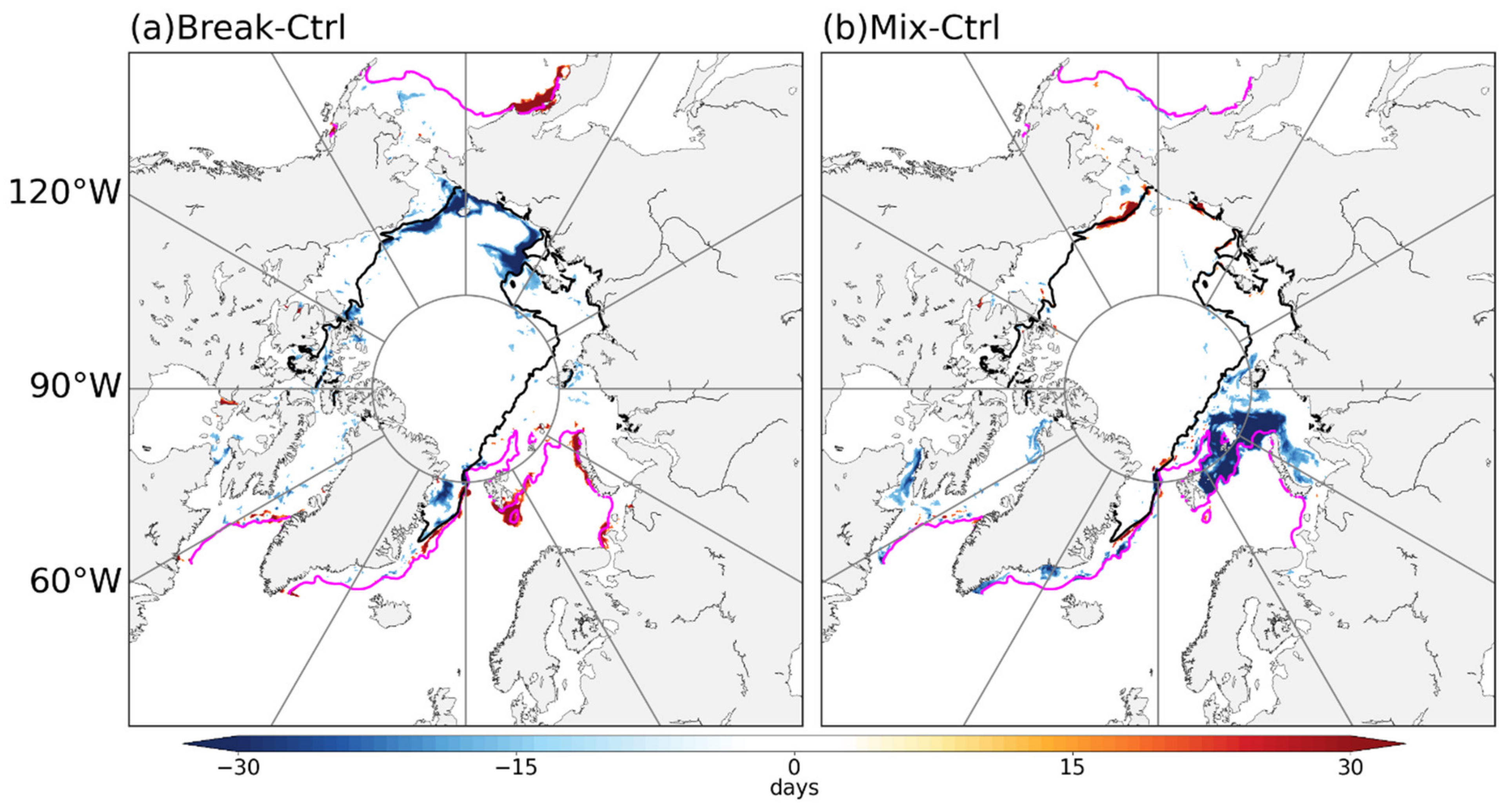
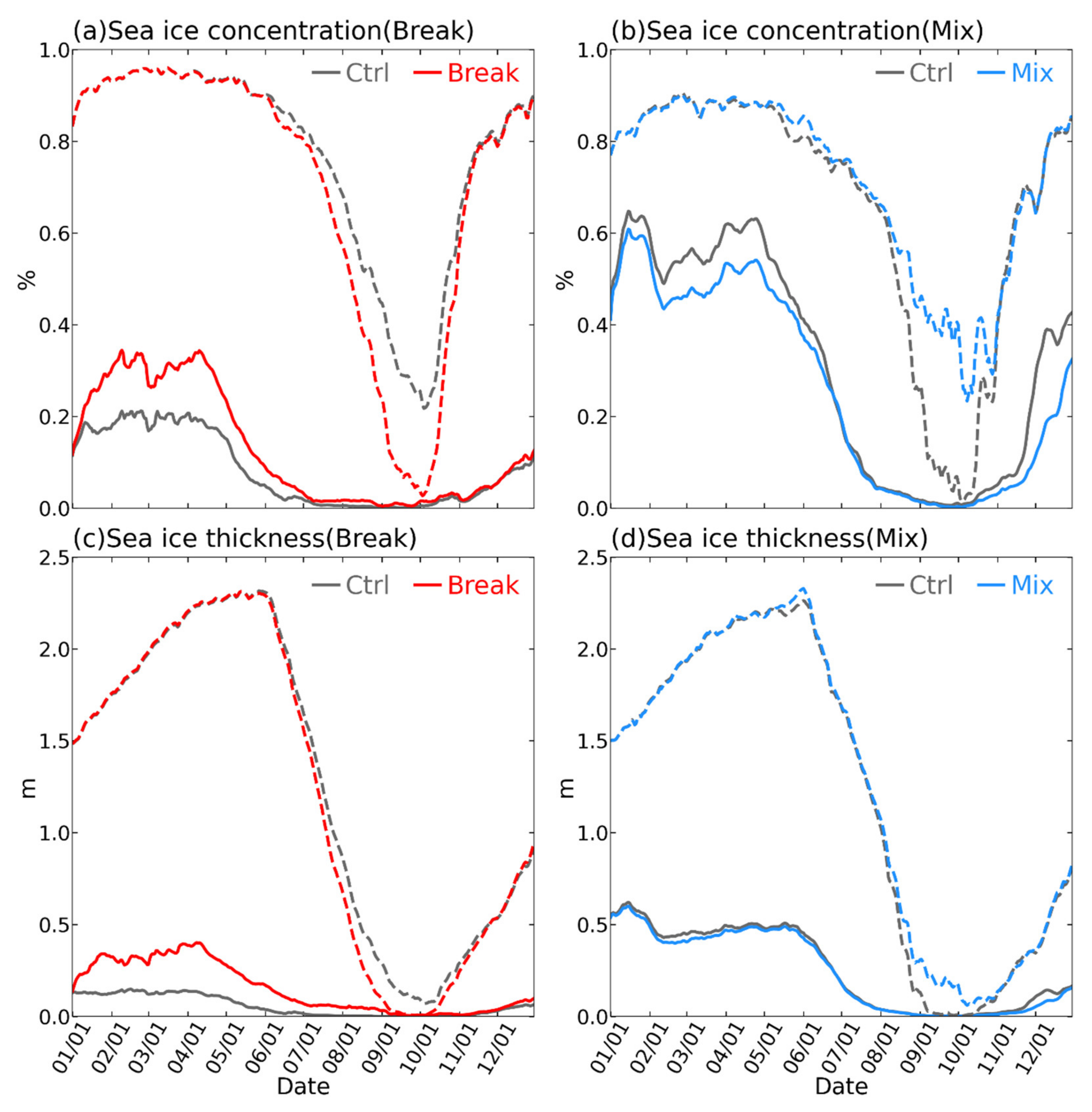
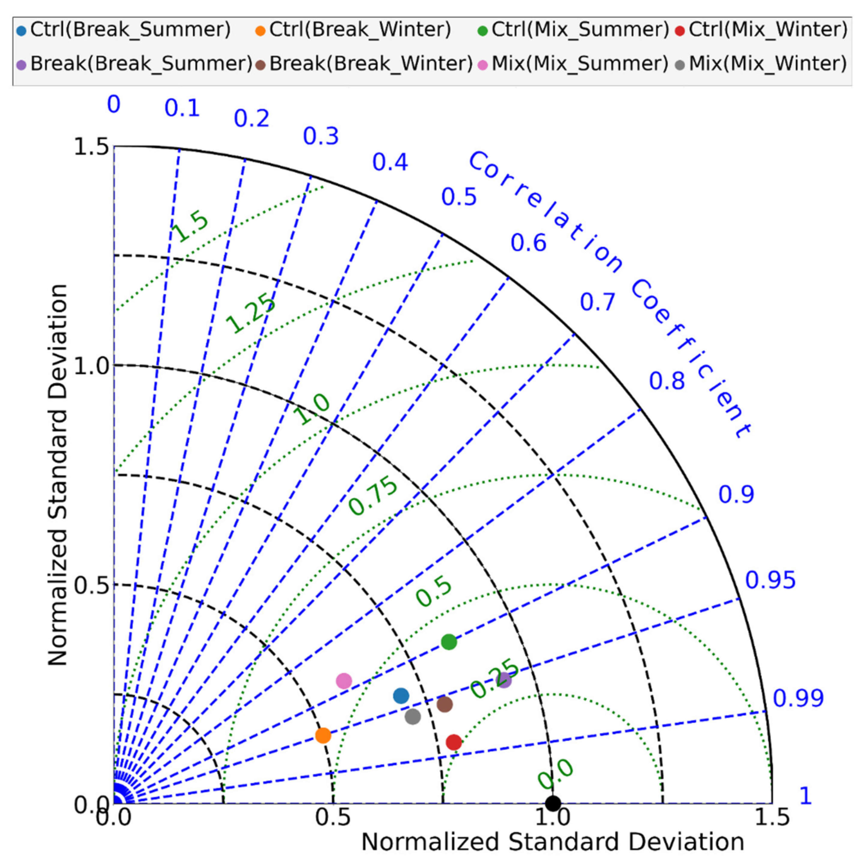
3.1. Wave Effects on the Sea Ice

Sea ice extent is a convenient variable to assess change in sea ice, not least because it can be measured by passive microwave (PM) sensors onboard satellites. Commonly, PM-derived sea ice concentration employs a cut-off of 15% to mark the ice edge. Sea ice volume is an important climate variable that integrates both sea ice thickness and extent. However, deriving sea ice volume from satellites observations depends on several assumptions, typically including ice and snow densities [73,82], hence reducing the accuracy of the derived ice thickness product. Also, ice thickness products are not continuous because of the lack of suitable observations during the sea ice melt season. The Pan-Arctic Ice Ocean Modeling and Assimilation System (PIOMAS) has thought to fill this gap by providing estimates of sea ice volume from simulations guided by observations [83]. It has been extensively validated through comparisons with a range of observations, such as US-Navy submarines, oceanographic moorings, and satellites [84].
The comparisons of the simulations from three experiments with satellite observations and PIOMAS reanalysis are shown in Figure 2. The daily evolution of sea ice extent from our model simulations is consistent with the satellite observations (Figure 2a). Arctic sea ice reaches its maximum extent around March at the end of winter, and the sea ice minimum occurs in September, at the end of the summer melting season. Compared to the satellite observations, the date of minimum and maximum sea ice extent is delayed by about 15 and 10 days later in the model simulations. As shown in Figure 2c, negative biases between the model simulations and observations dominate for most of the year, while positive bias occurs in August and September. Relative to the Ctrl experiment, the sea ice extent increases in the Break experiments from January to April and decreases from June to October. Therefore, the Break experiment decreases both negative biases during winter and positive biases in August and September between model simulations and observations. However, in the Mix experiment, the negative bias increases during the sea ice growth season. As shown in Figure 2b,d, the biases of sea ice volume between model simulations and PIOMAS reanalysis are very small from January to April. Compared to CS2SMOS observations, all of them overestimate the sea ice volume during this period. The sea ice volume from PIOMAS reanalysis are in good consistency with CS2SMOS observations from October to December, however, model simulations underestimate the sea ice volume in all three experiments. During the sea ice melt season from April to September, there are obvious model biases between model simulations and PIOMAS reanalysis. The decrease of sea ice volume starts from June and ends in October in the model simulations, which is about a month later than that in the PIOMAS reanalysis. Compared to the Ctrl experiment, there is no significant change in sea ice volume in the Mix experiment. However, in the Break experiment, the sea ice volume increases from January to May and decreases from August to October. Although the bias between the Break experiment and CS2SMOS becomes large, the minimum sea ice volume tends to be much closer to the PIOMAS reanalysis in August and September, which shows an improvement of sea ice volume simulation during the summer melt season.
Wave-induced mixing increases the mixed layer depth in the open water region during both ice growth and melt season (Figure S1), and wave can break sea ice in the MIZ (Figure S2). These processes play a different role in the sea ice evolution during sea ice growth and melt season. To further investigate the different results of the three experiments in the winter and summer season, the spatial distribution of sea ice concentration in March and September are compared in Figure 3. Sea ice extent is at its highest in March, when much of the Arctic Ocean is covered by sea ice extending into the Bering Sea, the Baffin Sea and some other subregions in the Ctrl experiment (Figure 3a). In the Break experiment (Figure 3b), we can see increases in sea ice concentration at the ice edge in the Bering Sea, the Baffin Sea and the Barents Sea, whereas in Mix (Figure 3c), sea ice concentration decreased significantly in the ice-covered areas of the Kara and the Barents seas. Consequently, the Break and Mix experiments account for the increase and decrease of sea ice extent, respectively, during winter. At sea ice minimum in September, the Bering, the Baffin, the Kara, the Barents seas and some other subregions are ice-free (Figure 3d). Break (Figure 3e) appears to promote sea ice retreat in the Chukchi and the East Siberian seas, significantly decreasing the September sea ice extent. In contrast, for Mix gives rise to sea ice concentration increases in these subregions (Figure 3f). The later increase has little contribution to the sea ice extent because it manifests in an area where sea ice is already prevalent with concentrations exceeding 15%.
The thickness of newly formed ice during the winter is generally below 0.5 m in the Bering, Baffin and Barents seas. For the Break experiment, regions of increase sea ice thickness mimic the increased sea ice concentration (Figure 3b and Figure 4b). They combine to an increase in sea ice volume during winter (Figure 2b). Although the decrease of sea ice concentration in the Kara and Barents seas is marked for the Mix experiment, the accompanying sea ice thickness exhibits only a small decrease (about 0.2 m) in those regions (Figure 4c). This is consistent with thin new ice in these subregions and hence little contribution to the sea ice volume, noting that most first-year sea ice melts during the following summer. In addition, much of the sea ice is thicker than 0.5 m by September (Figure 4d). Compared to the Ctrl experiment, we can see a significant decrease in the Chukchi Sea and the East Siberian Sea in the Break experiment (Figure 4e). The decrease exceeds 0.3 m in most areas, which accounts for most of the sea ice volume decrease in September (Figure 2b). For the Mix experiment, the increase in sea ice thickness exceeds 0.3 m in the Chukchi Sea.
The local sea ice conditions can be characterized by the length of the sea ice season (LSIS) [5], which is defined as the annual sum of days with sea ice concentration larger than 15% in one year. To examine the sea ice conditions in all three experiments, we compare the spatial distribution of LSIS in the model domain (Figure 5). It is noticeable that there is a two-rings dipole pattern in the differences of LSIS between the Break experiment and the Ctrl experiment (Figure 5a). The first ring, which is positive, indicates that the Break experiment has a longer LSIS. The positive ring occurs at the ice edge during the winter season, and the locations where LSIS is 15 days longer than that in the Ctrl experiment are referred to as Break_Winter, which are similar to the winter (March) impact on the distribution of ice concentration for the Break experiment (Figure 3b). Similarly, we can see a negative ring at the ice edge during summer, which is in the same location as the ice concentration distribution of the Break experiment during summer (Figure 3e). The locations where LSIS is 15 days shorter than that in the Ctrl experiment are referred to as Break_Summer. Therefore, this two-centre dipole pattern is useful to identify the location of the differences of sea ice concentration between the Break experiment and the Ctrl experiment in both winter and summer. The variations of sea ice concentration in the locations of Break_Winter and Break_Summer are the major contributions to the sea ice extent in the Break experiment. Likewise, a clear two-rings dipole pattern can also be found in the Mix experiment (Figure 5b), and the locations are similar to that for the respective distributions of ice concentration (Figure 3c,f). The positive ring occurs at the ice edge during the summer season, and the locations where LSIS is 15 days longer than that in the Ctrl experiment are referred to as Mix_Summer. During the winter season, we can find a negative ring at the ice edge. Accordingly, we define Mix_Winter by the locations where LSIS is 15 days shorter than that in the Ctrl experiment. As shown in the two-rings dipole pattern (Figure 5b), Mix_Summer and Mix_Winter also include almost all the locations that contribute most to the sea ice extent in the Mix experiment.
To explore the variation of sea ice concentration in the locations that significantly affect the sea ice extent in three experiments, the daily evolution of sea ice concentration averaged over the Break_Winter, Break_Summer, Mix_Winter and Mix_Summer are investigated (Figure 6a,b). In the Break_Winter, sea ice concentration in the Break experiment is larger than that in the Ctrl experiment from January to June, and the largest differences occur in February and April. The differences are very small after July when little sea ice survives in these locations. In the Break_Summer, there are no differences between Break and Ctrl during the sea ice growth season because all the locations within Break_Summer are covered by ice. Compared to the Ctrl experiment, we can see a distinct decrease in the Break experiment from June to November, and the sea ice concentration is very close to zero at the end of September, which indicates that the sea ice almost completely melts in these locations. In the Mix experiment, sea ice concentration decreases in the Mix_Winter during ice growth and increases from May to October in the Mix_Summer by comparison with the Ctrl experiment (Figure 6b). In the Mix_Summer locations, there is almost no sea ice at the end of September in the Ctrl experiment; however, sea ice concentration is larger than 20% in the Mix experiment. Comparison of sea ice concentration in three experiments shows that the effects of wave-induced sea ice break-up and associated mixing on sea ice concentration do not align. During winter, wave-induced sea ice break-up increases sea ice concentration, while wave-induced mixing decreases it. Wave-induced sea ice break-up accelerates sea ice melt during the summer season, whereas wave-induced mixing decelerates the loss of sea ice. Such opposing effects may also be found for the sea ice thickness that averaged over the Break_Winter, Break_Summer, Mix_Winter and Mix_Summer in three experiments (Figure 6c,d). Sea ice thickness increases in the Break_Winter and decreases in the Break_Summer by comparison with the Ctrl experiment. The maximum increase and decrease are 0.84 m in winter and 0.2 m in summer, respectively. In the Mix experiment, we can see a very slight decrease for the Mix_Winter, which indicates that wave-induced mixing retards the new ice formation. In the Mix_Summer, there is an increase from August to October because wave-induced mixing retards sea ice melt during summer.
A Taylor diagram (Appendix A, Equations (A1)–(A3)) is used to examine the performance skills of three experiments in the Break_Summer, Break_Winter, Mix_Summer and Mix_Winter locations. As shown in Figure 7, the correlation coefficients in almost all the locations are larger than 0.9 and have a low centred root mean square errors (CRMSE) of less than 0.5. In the Break experiment, we can see an increase of correlation coefficient and a decrease of CRMSE in both the Break_Summer and Break_Winter by comparison with the Ctrl experiment. Sea ice concentration in the Break experiment is closer to the observation, indicating that wave-induced sea ice break-up improves the sea ice simulation in both the sea ice growth and melt season. The Ctrl experiment underestimates the sea ice extent in the ice growth season and overestimates the sea ice extent during the ice melt season (Figure 2). Compared to the Ctrl experiment, wave-induced mixing decreases sea ice concentration in winter and increases sea ice concentration in summer (Figure 6b). Therefore, the wave-induced mixing has a negative role in the sea ice simulation, increasing the CRMSE and decreasing the correlation coefficient in both Mix_Summer and Mix_Winter.

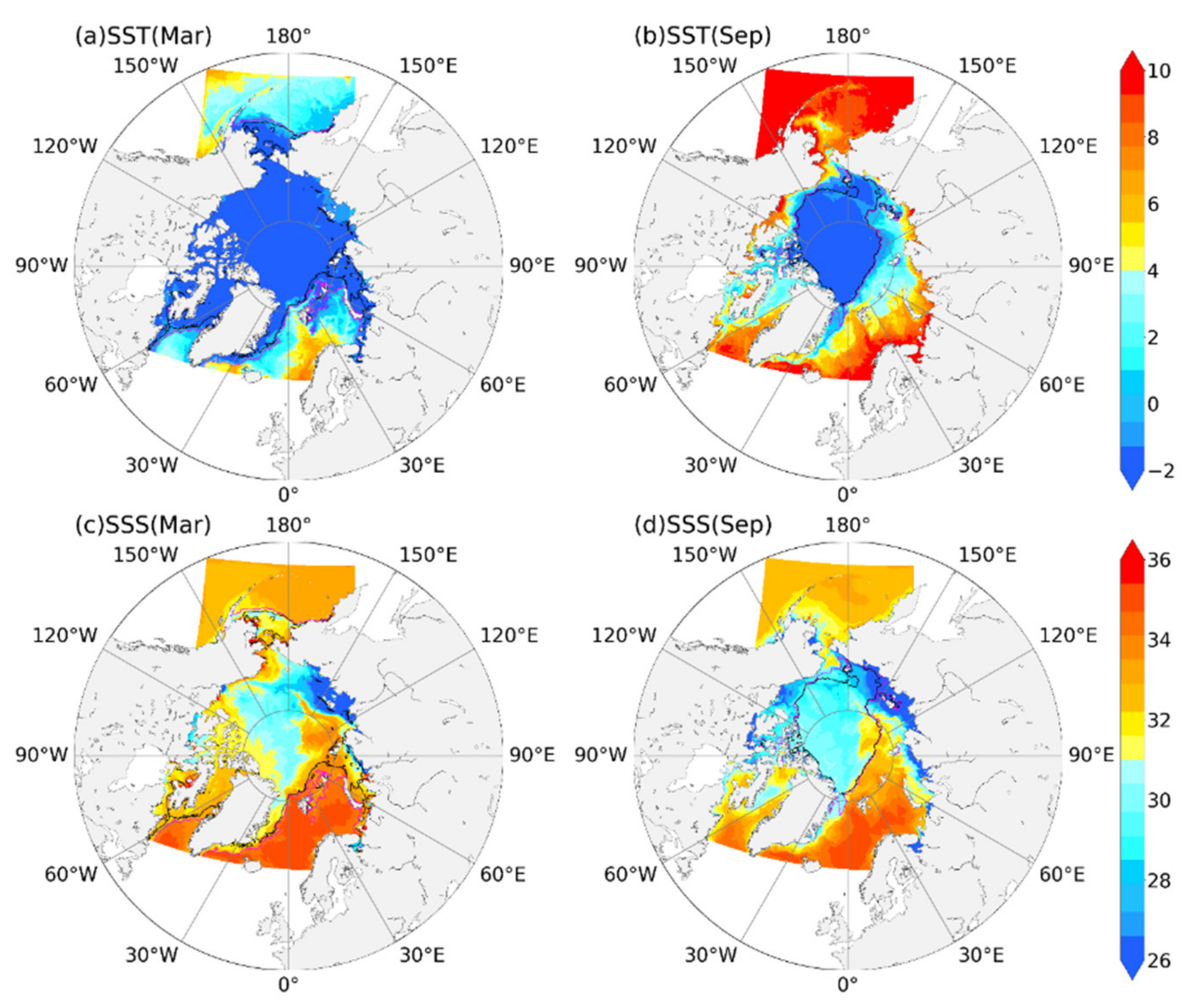
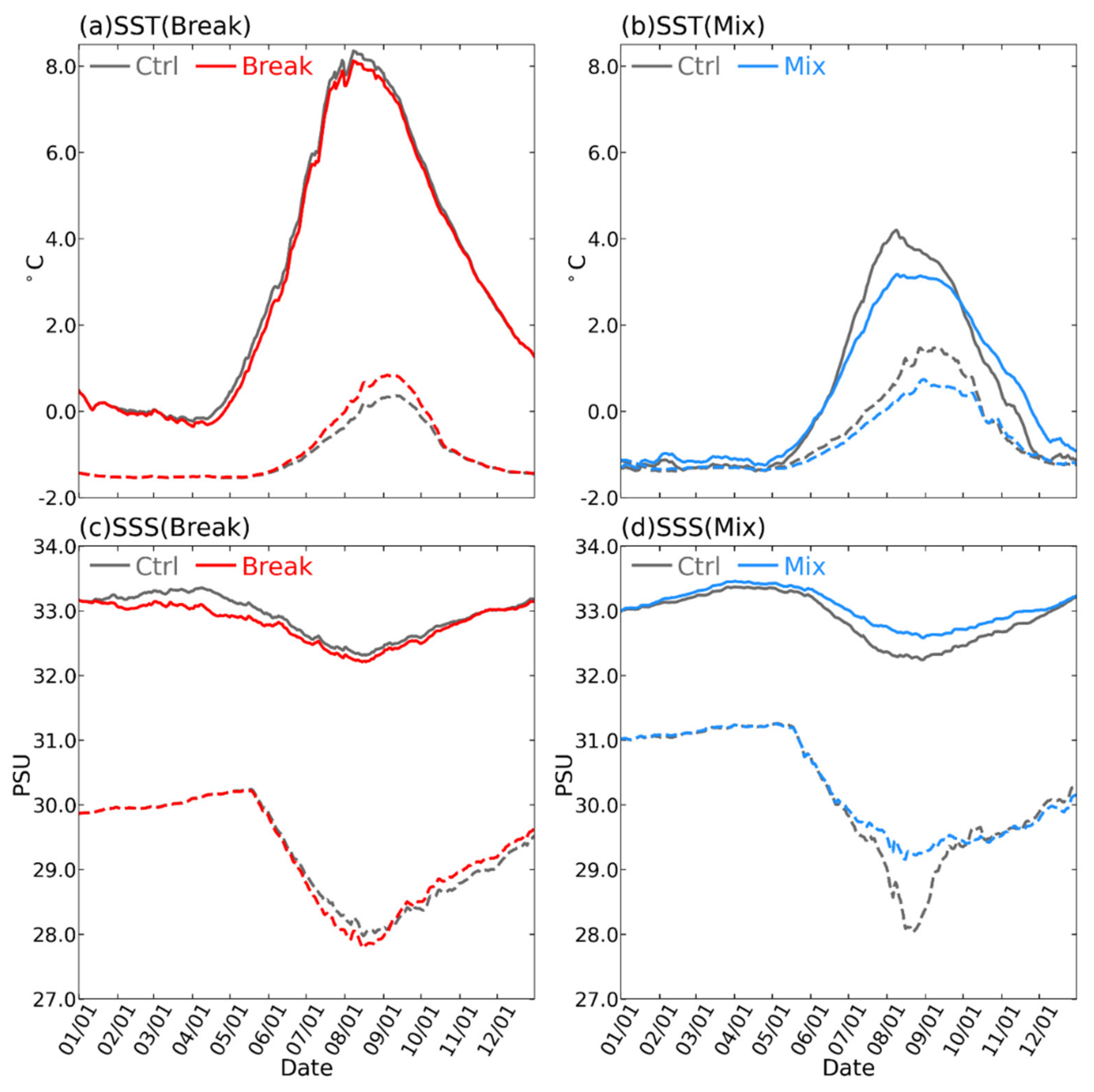
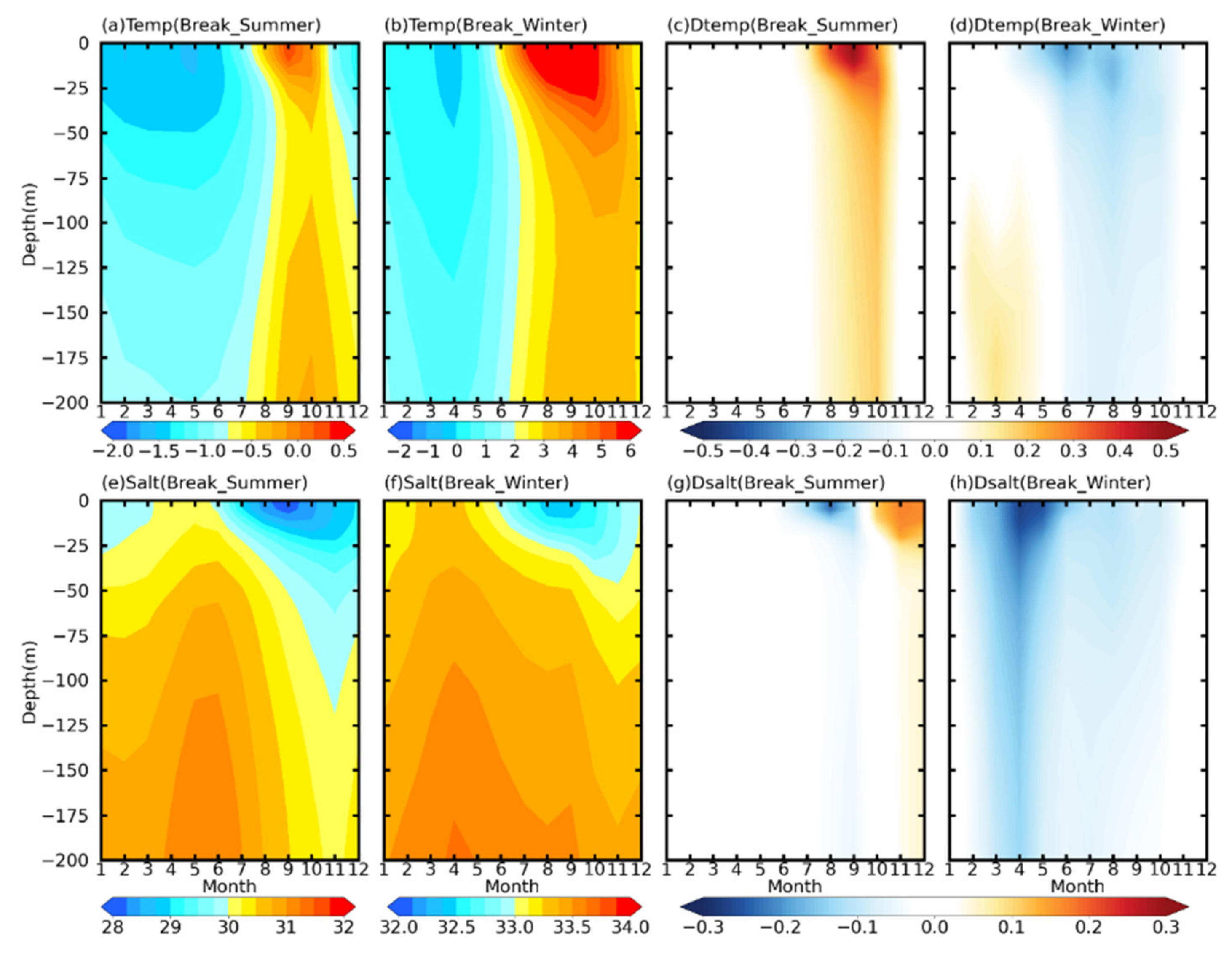
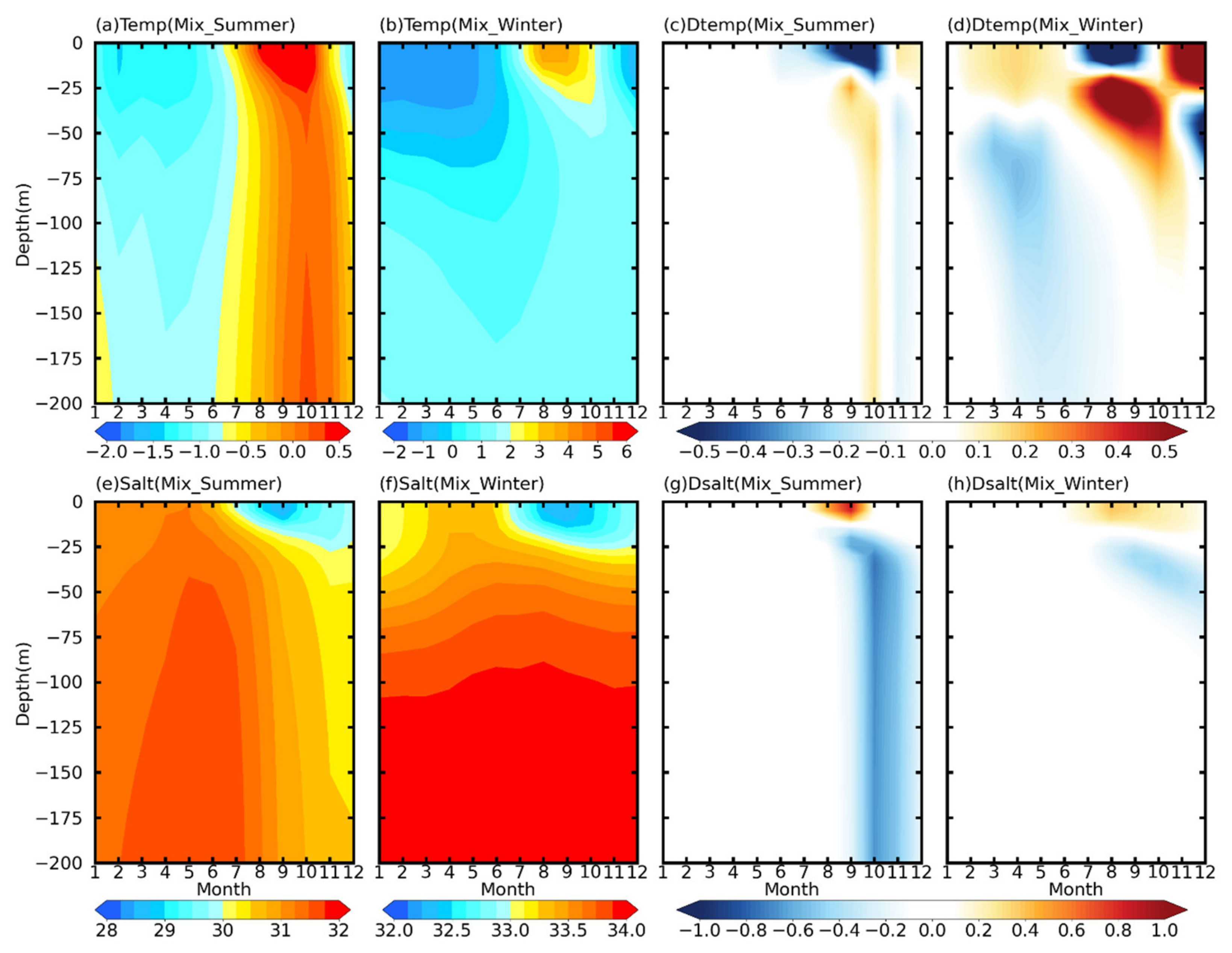
3.2. Wave Effects on the Ocean

While in the coupled ice-ocean model, sea surface temperature and ocean salinity strongly modulate the sea ice evolution and the sea ice concentration, in turn, affects the heat and fresh fluxes between the ocean and atmosphere. On the one hand, the heat flux at the ice-ocean interface is highly related to the sea surface temperature and salinity. The sea ice module in ROMS is a simple one-layer ice and snow thermodynamics with a molecular sublayer under the ice [30]. At the bottom of the ice, the heat conduction is Qio = (2ki/hi) (T0T1), where ki, hi, T0, T1 are the ice thermal conductivity, sea ice thickness, sea surface temperature and the temperature of the interior of the ice, respectively. In the presence of ice, the surface ocean is assumed to be at the freezing temperature for the surface salinity: T0 = −0.0543S0, where S0 is the surface salinity in the ocean. Therefore, the heat flux at the ice-ocean interface and associated sea ice evolutions are highly related to the sea surface temperature and ocean salinity. On the other hand, the seasonal variation of the distribution of sea surface temperature and salinity in the Arctic Ocean is largely influenced by the sea ice (Figure 8). During the ice growth season, most subregions in the Arctic Ocean are covered by sea ice, where the sea surface temperature is lower than that in the ice-free region (Figure 8a). Here, the variation of sea surface temperature in the MIZ will affect the sea ice melting and refreezing. During the ice melt season, first-year ice melts because of the increased input of solar radiation. Sea surface temperature in the ice-free area also increases fast through absorption of radiative heat, therefore, it exceeds that of the ice-covered regions (Figure 8b). The warm water has the potential to hence the loss of sea ice through the lateral melt. Sea surface salinity in the ice-covered area is also quite different from the ice-free regions. In winter, sea surface salinities in open water regions of the Barents and the Greenland seas are much higher than for other regions (Figure 8c). The freezing temperature decreases with increasing salinity water, which will retard the formation of sea ice. In summer, the ocean is covered by fresh water where ice melts (Figure 8d).
Figure 9 shows the monthly evolutions of sea surface temperature and salinity averaged over the Break_Winter, Break_Summer, Mix_Winter and Mix_Summer locations. In the Break experiment, the sea ice cover increases over the cold ocean in winter because new sea ice may form where sea ice break-up occurs. In the Break_Winter locations, both sea ice concentration and sea ice thickness increase during the sea ice growth season compared to the Ctrl run (Figure 6a,c). Therefore, in the subsequent sea ice melt season, it requires more heat to melt the increased sea ice, resulting in a decrease in sea surface temperature in the Break_Winter locations compared to the Ctrl experiment (Figure 9a). In the Break_Summer locations, more sea ice melt in summer, the sea surface temperature increases by absorbing more solar radiation (Figure 9a). In the Mix experiment, wave-induced mixing enhances the exchange of heat and salt between the surface and subsurface layers due to increased mixed layer depth (Figure S1), resulting in increased sea surface temperature during sea ice growth and decreased sea surface temperature in summer (Figure 9b). Likewise, sea surface salinities also have corresponding variations. Figure 9c shows a decrease in sea surface salinity in the Break_Winter locations throughout the year. Whereas, in the Break_Summer locations, there is a decrease in summer and followed by an increase in the following months. Wave-induced mixing increases the sea surface salinity in the Mix_Winter locations all the year and significantly increases it during summer in the Mix_Summer locations (Figure 9d).
To further investigate the dynamics that induced the variations of sea surface temperature and salinity in the Break experiment, we diagnose the temperatures and salinity profiles of the upper 200 m that are averaged over the Break_Winter and Break_Summer locations. Figure 10a shows the temperature profile in the Ctrl experiment in the Break_Summer locations. Due to the melt of sea ice in summer, more heat enters into the ocean and significantly increase the temperatures over the upper 200 m. Wave-induced sea ice breakup decreases the sea ice concentration, which will increase the area of open water and further increases the input of heat fluxes into the ocean. Therefore, compared to the Ctrl experiment, the temperature in the upper 200 m increase in the Break_Summer, particularly in the upper 50 m (Figure 10c). In the Break_Winter locations, the temperature is very low and uniform in the upper 200 m in winter (Figure 10b). As discussed in Section 3.1, wave-induced sea ice break-up increases the sea ice concentration because the broken sea ice may refreeze in the areas where the sea surface temperature is lower than the freezing temperature. The refrozen of sea ice hinders ocean heat loss during the cold winter season, leading to a minor increase of temperature in the subsurface layer in the Break_Winter locations in winter (Figure 10d). However, more heat is required to melt the increased sea ice during the summer season, resulting in a decrease in temperature in the following month (Figure 10d). Figure 10e shows a low salinity core in the upper 20 m in the Break_Summer locations, which results from the melt of sea ice. The break-up of sea ice accelerates the ice melt in summer, therefore, there is more fresh water in the surface ocean. As the freezing point is much lower in low salinity water, these fresh water refreezes in the Break_Summer locations during the ice growth season. Then, more salt is ejected back into the ocean, increasing the salinity of the surface water, as shown by a high salinity core (Figure 10g). In the Break_Winter locations, the upper ocean is covered by high salinity water that is larger than 33.0 (Figure 10f). As shown in Figure 5a and Figure 8c, the Break_Winter locations are surrounded by much higher salinity water in the ice-free ocean. The increase of sea ice cover may impede the high salinity water flow into the Break_Winter locations, therefore, we can see a decrease of salinity in the upper 200 m, which is enhanced in the upper 50 m (Figure 10h). The freezing temperature in low salinity water is also lower, facilitating the increase in sea ice thickness (Figure 6c).
Figure 11 shows the effects of wave-induced mixing on the temperature and salinity profile in the upper 200 m over the Mix_Winter and Mix_Summer locations. We identify a warm water column in the upper 200 m in the Mix_Summer locations in summer (Figure 11a). The effects of wave-induced mixing, however, differ from those of wave-induced sea ice break-up. Surface wave mixing captures heat from the solar-warmed surface and mixes it into the deeper mixed layer in summer [17,63], increasing the mixed layer depth (Figure S1) and further enhancing the heat and fresh fluxes exchange between the surface and subsurface layer. Accordingly, there is a cooling of the ocean surface in the upper 20 m and an increase in ocean heat content under 20 m in summer compared with the Ctrl experiment (Figure 11c). The cooling of the surface ocean reduces the sea ice melt and thereby increases sea ice concentration in the Mix_Summer locations. In winter, the surface ocean is much cooler in the upper 30 m than the subsurface because of the loss as conductive (Figure 11b). Surface wave mixing takes the subsurface warm water into the surface ocean, increasing the ocean surface temperature and decreasing the subsurface temperature compared with the Ctrl experiment (Figure 11d). The warming of the surface ocean impedes the formation of new ice, decreasing the sea ice concentration in the Mix_Winter. The ocean in the upper 20 m in the Mix_Summer locations is covered by fresh water due to summer sea ice melt (Figure 11e). The surface wave mixes the fresh water downward into the subsurface, producing an increase of salinity in the surface ocean and a decrease of salinity in the subsurface (Figure 11g). The cold and saline surface ocean make the sea ice in the Mix_Summer locations more difficult to melt in summer. During the winter season, the vertical distribution of salinity in the Mix_Winter is very uniform in the ice-covered area, therefore, the contribution of wave-induced mixing on salinity is limit (Figure 11f,h). During the sea ice melt season, the differences of salinity between the surface and subsurface layers are obvious in the Mix_Winter locations. In this case, the surface wave also mixes the water column in the upper 100 m (Figure 11h).

4. Discussion

Similar to many ice models [85], our results exhibit biases in sea ice cover between our model simulations and observations. As our objective is to investigate the impact of waves on sea ice evolution, similar to those of Liang and Losch [13] and Moorman et al. [86], here we conducted sensitivity experiments. Our results are based on analyzing the differences between the sensitivity Break and Mix experiments and the Ctrl experiment, which are almost independent of the model biases, as shown by Figure 5. Hence, the model biases have a negligible effect on the conclusion of our qualitative study.
Previous studies explored the wave-induced mixing on Antarctic sea ice in an ice-ocean coupled model [17]. Waves are considered as external forcing and are taken from a wave hindcast from the WAVEWATCH III model. Under these circumstances, sea ice concentration biases between the ice model and the wave model may produce gaps or overlaps in some areas between the ice data and wave data. However, this has not been taken into account here. If the sea ice model overestimates the sea ice concentration, wave energy will remain in the ice-covered areas. To remove these artificial wave effects, both the wave-induced sea ice break-up and mixing are constrained within the MIZ in this study. It is noted that sea ice break-up events do not occur in the whole MIZ region (Figure S2), indicating that this approach may effectively remove artificial wave effects. An underestimation of sea ice concentration in the ice model will reduce the wave effects because there are no wave data in the areas where the artificial lower sea ice concentration exists. A fully coupled ice-ocean-wave model will remove the gaps and overlaps between wave and ice models, which needs to be developed in our future work but is outside the scope of this study.
In this study, the wave-induced mixing and wave-induced sea ice break up are two independent sensitivity experiments. In the wave-induced mixing experiment, we do not consider wave-induced sea ice break up. Similarly, we do not consider wave-induced mixing in the wave-induced sea ice break up experiment. These setups are commonly used to investigate the independent effect of each sensitivity experiment. In our parameterization, an extra term PW was introduced to include the wave-induced mixing. While wave propagates into the MIZ, Hs decays exponentially with distance from the sea ice edge [87], resulting in a significant decrease in PW in the ice-covered area. The wave-induced mixing parameterization does not depend on ice-cover. Full details about the parameterization of PW can be found in Ghantous and Babanin [61], and its application of wave-induced mixing on Antarctic sea ice simulation can be found in Thomas et al. [17].
Wave-induced sea ice break-up and mixing play different roles in affecting the sea ice evolution. In winter, wave-induced sea ice break-up increases sea ice cover, however, wave mixing impedes sea ice formation. In summer, they operate in the opposite direction. How much improvement they can make on sea ice simulation results highly depends on the biases of sea ice extent between the ice model and the observations. If the ice model overestimates sea ice extent all the year [17], wave-induced mixing will reduce the bias during ice formation season because wave mixing increases the temperature in the surface ocean that retards the sea ice increase. In this study, the ROMS-Budgell model underestimates sea ice extent in winter and produces more sea ice than observed during summer. Therefore, we can see an improvement in the Break experiment, whereas wave-induced mixing amplifies the biases between the model simulation and observations. As shown in Roach et al. [88] and Shu et al. [85], large uncertainties exist in the Coupled Model Intercomparison Project Phase 6 (CMIP6). The CMIP6 models overestimate interannual variability at the winter maximum but underestimate summer sea ice area in the Antarctic [88], and were unable to reproduce the faster decline of Arctic sea ice extent in summer [85]. This study introduces two methods to directly include the wave effects into the climate models, which in turn will act to reduce the model biases and improve the sea ice simulation.

5. Conclusions

In this study, we have investigated the wave effects on the Arctic sea ice simulation using a high-resolution coupled ice-ocean model. Two independent parameterizations are implemented to represent the wave-induced sea ice break-up and mixing. The inclusion of these parameterizations shows a notable impact on both Arctic sea ice extent and volume with different dynamical mechanisms. During the sea ice growth, heat is lost from the ocean to the atmosphere, reducing the temperature of the surface ocean. If sea ice break-up occurs in the areas with sea surface temperature lower than the freezing temperature, the exposed ocean will refreeze again to increase the ice-covered area. Our results show that wave-induced sea ice break-up increases both the sea ice concentration and thickness in the Bering Sea, the Baffin Sea and the Barents Sea. Wave-induced vertical mixing takes the subsurface heat upward to warm the surface ocean, decelerating the sea ice formation in the Barents Sea. During the sea ice melt season, the ocean absorbs solar radiation from the atmosphere to increase the sea surface temperature. In the Chukchi Sea and the East Siberian Sea, both sea ice concentration and thickness significantly decrease as the wave-induced sea ice break-up increases the heat fluxes input from the atmosphere into the ocean. In the Mix experiment, waves mix the surface heat into the subsurface layer, decelerating the sea ice melt in the Chukchi Sea and the East Siberian Sea. As such, these processes play opposite roles in sea ice evolution. Because our model underestimates sea ice extent in winter and produces more sea ice in summer, the biases between model simulations and observation become larger due to the wave-induced mixing. However, we can find an obvious improvement in sea ice simulation due to the wave-induced sea ice break-up in the Break experiment.
In the coupled ice-ocean model, we have also examined the wave effects on the ocean. In the Break experiment, sea ice break-up increases the area of open water and sea ice melt in summer, increasing the temperature and decreasing the salinity in the upper ocean. In winter, the refreeze of sea ice decelerates the loss of heat from the ocean to the atmosphere and also impedes the high salinity water flow into the ice-covered ocean. In the Mix experiment, our results show that wave-induced mixing plays an important role in the exchange of heat and freshwater fluxes between the surface layer and subsurface layer. In summer, the surface ocean in the upper 20 m cools and becomes saltier because of the wave-induced mixing, followed by the warmer and fresher water below this layer. In winter, the subsurface warm water is taken into the surface ocean by the surface wave mixing, leading to a warmer surface and cooler subsurface. Both the wave-induced sea ice break-up and mixing have notable impacts on the upper 200 m ocean.
Our results suggest that the inclusion of wave-induced sea ice break-up and mixing significantly affects the sea ice simulation in the MIZ. The improvements of including wave parameterizations on sea ice simulation results are highly related to the sea ice extent biases between the ice model and the observations. We also reveal the dynamics of wave effects on the surface ocean in the Arctic Ocean, associated with sea ice evolution. This study provides two independent parameterizations to reduce the model bias by including the wave effects in the sea ice simulation, with important implications for the future sea ice model development.

Supplementary Materials

The following are available online at https://www.mdpi.com/article/10.3390/jmse9040365/s1, Figure S1: The differences of mixed layer depth between Mix and Ctrl. Figure S2: The locations of sea ice break-up event occur.

Author Contributions

Conceptualization, A.V.B. and J.L.; methodology, Q.L. and J.J.V.; software, J.L.; validation, J.L.; formal analysis, J.L.; investigation, J.L.; resources, J.L. and Q.L.; data curation, J.L. and Q.L.; writing—original draft preparation, J.L.; writing—review and editing, Q.L., J.J.V., P.H. and Y.T.; visualization, J.L.; supervision, A.V.B.; project administration, A.V.B.; funding acquisition, A.V.B., J.J.V., P.H. All authors have read and agreed to the published version of the manuscript.

Funding

J.L., A.V.B. and Q.L. acknowledge ONR Global Grant N00014-17-1-3021-A00001; J.J.V., A.V.B. and P.H. were supported by the Australian Antarctic Program under project 4593 with additional contributions from project 4506.

Institutional Review Board Statement

Not applicable.

Informed Consent Statement

Not applicable.

Data Availability Statement

Estimating the Circulation and Climate of the Ocean, Phase II (ECCO2) cube92 reanalysis product can be obtained from https://www.ecco-group.org/products.htm (accessed on 29 March 2021). NOAA/NSIDC Climate Data Record of Passive Microwave Sea Ice Concentration, Version 3 datasets are taken from https://nsidc.org/data/G02202/versions/3 (accessed on 29 March 2021). CS2SMOS product version v202 is available at ftp://ftp.awi.de/sea_ice/product/cryosat2_smos/v202/nh/ (accessed on 29 March 2021). ERA5 datasets are provided by https://cds.climate.copernicus.eu/#!/home (accessed on 29 March 2021).

Acknowledgments

This research was undertaken with the assistance of resources and services from the National Computational Infrastructure (NCI), which is supported by the Australian Government. The authors would also like to thank Rajesh Kumar and Kate Hedström for providing us with the ROMS core sea ice model code, the grid, river and tide data.

Conflicts of Interest

The authors declare no conflict of interest.

Appendix A

Taylor diagram provides a concise statistical summary of how closely the model patterns match observations [89] in terms of their correlation coefficients (R), their centered root mean square errors (CRMSE), their standard deviations (STD). The statistics that appeared on the Taylor diagram can be normalized by the standard deviation of the corresponding observations, which has been widely used in the model evaluation [80,81,82,83,84,85,86,87,88,89,90,91,92,93]. In the normalized Taylor diagrams, R, CRMSE and STD are given below:
R = 1 N n = 1 N ( f n f ¯ ) ( r n r ¯ ) n = 1 N ( f n f ¯ ) 2 n = 1 N ( r n r ¯ ) 2
C R M S E = n = 1 N ( f n f ¯ ) ( r n r ¯ ) 2 n = 1 N ( r n r ¯ ) 2
S T D = n = 1 N ( f n f ¯ ) 2 n = 1 N ( r n r ¯ ) 2
where f ¯ and r ¯ are the mean values of the model simulation f and the observation r with a sample size of N, respectively.

References

  1. Curry, J.A.; Schramm, J.L.; Ebert, E.E. Sea Ice-Albedo Climate Feedback Mechanism. J. Clim. 1995, 8, 240–247. [Google Scholar] [CrossRef]
  2. Thomson, J.; Rogers, W.E. Swell and sea in the emerging Arctic Ocean. Geophys. Res. Lett. 2014, 41, 3136–3140. [Google Scholar] [CrossRef]
  3. Squire, V.A. Ocean wave interactions with sea ice: A reappraisal. Annu. Rev. Fluid Mech. 2020, 52, 37–60. [Google Scholar] [CrossRef] [Green Version]
  4. Huang, L.; Tuhkuri, J.; Igrec, B.; Li, M.; Stagonas, D.; Toffoli, A.; Cardiff, P.; Thomas, G. Ship resistance when operating in floating ice floes: A combined CFD&DEM approach. Mar. Struct. 2020, 74, 102817. [Google Scholar]
  5. Ni, B.Y.; Han, D.F.; Di, S.C.; Xue, Y.Z. On the development of ice-water-structure interaction. J. Hydrodyn. 2020, 32, 629–652. [Google Scholar] [CrossRef]
  6. Bennetts, L.G.; Squire, V.A. Wave scattering by multiple rows of circular ice floes. J. Fluid Mech. 2009, 639, 213–238. [Google Scholar] [CrossRef]
  7. Bennetts, L.G.; Peter, M.A.; Squire, V.A.; Meylan, M.H. A three-dimensional model of wave attenuation in the marginal ice zone. J. Geophys. Res. Oceans 2010, 115, C12043. [Google Scholar] [CrossRef] [Green Version]
  8. Bennetts, L.G.; Williams, T.D.; Bennetts, L.G.; Williams, T.D. Water wave transmission by an array of floating discs. Proc. R. Soc. A. 2015, 471, 20140698. [Google Scholar] [CrossRef] [Green Version]
  9. Montiel, F.; Squire, V.A.; Bennetts, L.G. Attenuation and directional spreading of ocean wave spectra in the marginal ice zone. J. Fluid Mech. 2016, 790, 492–522. [Google Scholar] [CrossRef] [Green Version]
  10. Huang, L.; Ren, K.; Li, M.; Tuković, Ž.; Cardiff, P.; Thomas, G. Fluid-structure interaction of a large ice sheet in waves. Ocean Eng. 2019, 182, 102–111. [Google Scholar] [CrossRef] [Green Version]
  11. Goosse, H.; Deleersnijder, E.; Fichefet, T.; England, M. Sensitivity of a global coupled ocean-sea ice model to the parameterization of vertical mixing. J. Geophys. Res. Oceans 1999, 104, 13681–13695. [Google Scholar] [CrossRef] [Green Version]
  12. Zhang, J.; Steele, M. Effect of vertical mixing on the Atlantic Water layer circulation in the Arctic Ocean. J. Geophys. Res. Oceans 2007, 112, C04S04. [Google Scholar] [CrossRef]
  13. Liang, X.; Losch, M. On the effects of increased vertical mixing on the Arctic Ocean and sea ice. J. Geophys. Res. Oceans 2018, 123, 9266–9282. [Google Scholar] [CrossRef] [Green Version]
  14. Dumont, D.; Kohout, A.; Bertino, L. A wave-based model for the marginal ice zone including a floe breaking parameterization. J. Geophys. Res. Oceans 2011, 116. [Google Scholar] [CrossRef] [Green Version]
  15. Squire, V.A.; Dugan, J.P.; Wadhams, P.; Rottier, P.J.; Liu, A.K. Of Ocean Waves and Sea Ice. Annu. Rev. Fluid Mech. 1995, 27, 115–168. [Google Scholar] [CrossRef]
  16. Steele, M. Sea ice melting and floe geometry in a simple ice-ocean model. J. Geophys. Res. Oceans 1992, 97, 17729–17738. [Google Scholar] [CrossRef]
  17. Thomas, S.; Babanin, A.V.; Walsh, K.J.; Stoney, L.; Heil, P. Effect of wave-induced mixing on Antarctic sea ice in a high-resolution ocean model. Ocean. Dyn. 2019, 69, 737–746. [Google Scholar] [CrossRef]
  18. Komuro, Y. The Impact of Surface Mixing on the Arctic River Water Distribution and Stratification in a Global Ice–Ocean Model. J. Clim. 2014, 27, 4359–4370. [Google Scholar] [CrossRef]
  19. Bateson, A.W.; Feltham, D.L.; Schröder, D.; Hosekova, L.; Ridley, J.K.; Aksenov, Y. Impact of sea ice floe size distribution on seasonal fragmentation and melt of Arctic sea ice. Cryosphere 2020, 14, 403–428. [Google Scholar] [CrossRef] [Green Version]
  20. Boutin, G.; Lique, C.; Ardhuin, F.; Rousset, C.; Talandier, C.; Accensi, M.; Girard-Ardhuin, F. Towards a coupled model to investigate wave–sea ice interactions in the Arctic marginal ice zone. Cryosphere 2020, 14, 709–735. [Google Scholar] [CrossRef] [Green Version]
  21. Stern, H.L.; Schweiger, A.J.; Stark, M.; Zhang, J.; Steele, M.; Hwang, B. Seasonal evolution of the sea-ice floe size distribution in the Beaufort and Chukchi seas. Elem. Sci. Anth. 2018, 6, 48. [Google Scholar] [CrossRef]
  22. Herman, A. Wave-induced surge motion and collisions of sea ice floes: Finite-floe-size effects. J. Geophys. Res. Oceans 2018, 123, 7472–7494. [Google Scholar] [CrossRef]
  23. Stern, H.L.; Schweiger, A.J.; Zhang, J.; Steele, M. On reconciling disparate studies of the sea-ice floe size distribution. Elem. Sci. Anth. 2018, 6, 49. [Google Scholar] [CrossRef]
  24. Voermans, J.J.; Rabault, J.; Filchuk, K.; Ryzhov, I.; Heil, P.; Marchenko, A.; Collins, C.O., III; Dabboor, M.; Sutherland, G.; Babanin, A.V. Experimental evidence for a universal threshold characterizing wave-induced sea ice break-up. Cryosphere 2020, 14, 4265–4278. [Google Scholar] [CrossRef]
  25. Shchepetkin, A.F.; McWilliams, J.C. The regional oceanic modeling system (ROMS): A split-explicit, free-surface, topography-following-coordinate oceanic model. Ocean Model. 2005, 9, 347–404. [Google Scholar] [CrossRef]
  26. Budgell, W.P. Numerical simulation of ice-ocean variability in the Barents Sea region. Ocean Dyn. 2005, 55, 370–387. [Google Scholar] [CrossRef]
  27. Hedström, K.S. Technical Manual for a Coupled Sea-Ice/Ocean Circulation Model, (Version 5); OCS Study BOEM 2018-007; U.S. Department of the Interior, Bureau of Ocean Energy Management, Alaska OCS Region: Anchorage, AK, USA, 2018; 182p.
  28. Hunke, E.C. Viscous-Plastic Sea Ice Dynamics with the EVP Model: Linearization Issues. J. Comput. Phys. 2001, 170, 18–38. [Google Scholar] [CrossRef]
  29. Hunke, E.C.; Dukowicz, J.K. An Elastic-Viscous-Plastic Model for Sea Ice Dynamics. J. Phys. Oceanogr. 1997, 27, 1849–1867. [Google Scholar] [CrossRef] [Green Version]
  30. Mellor, G.L.; Kantha, L. An ice-ocean coupled model. J. Geophys. Res. Oceans 1989, 94, 10937–10954. [Google Scholar] [CrossRef]
  31. Dong, C.; Gao, X.; Zhang, Y.; Yang, J.; Zhang, H.; Chao, Y. Multiple-Scale Variations of Sea Ice and Ocean Circulation in the Bering Sea Using Remote Sensing Observations and Numerical Modeling. Remote Sens. 2019, 11, 1484. [Google Scholar] [CrossRef] [Green Version]
  32. Durski, S.M.; Kurapov, A.L. A high-resolution coupled ice-ocean model of winter circulation on the bering sea shelf. Part I: Ice model refinements and skill assessments. Ocean Model. 2019, 133, 145–161. [Google Scholar] [CrossRef]
  33. Liang, X.; Yang, Q.; Nerger, L.; Losa, S.N.; Zhao, B.; Zheng, F.; Zhang, L.; Wu, L. Assimilating Copernicus SST Data into a Pan-Arctic Ice–Ocean Coupled Model with a Local SEIK Filter. J. Atmos. Ocean. Technol. 2017, 34, 1985–1999. [Google Scholar] [CrossRef]
  34. Melsom, A.; Lien, V.S.; Budgell, W.P. Using the Regional Ocean Modeling System (ROMS) to improve the ocean circulation from a GCM 20th century simulation. Ocean Dyn. 2009, 59, 969. [Google Scholar] [CrossRef] [Green Version]
  35. Wang, K.; Debernard, J.; Sperrevik, A.K.; Isachsen, P.E.; Lavergne, T. A combined optimal interpolation and nudging scheme to assimilate OSISAF sea-ice concentration into ROMS. Ann. Glaciol. 2013, 54, 8–12. [Google Scholar] [CrossRef] [Green Version]
  36. Yang, C.-Y.; Liu, J.; Xu, S. Seasonal Arctic Sea Ice Prediction Using a Newly Developed Fully Coupled Regional Model With the Assimilation of Satellite Sea Ice Observations. J. Adv. Model. Earth Syst. 2020, 12, e2019MS001938. [Google Scholar] [CrossRef] [Green Version]
  37. Dinniman, M.S.; Klinck, J.M.; Smith, W.O., Jr. A model study of Circumpolar Deep Water on the West Antarctic Peninsula and Ross Sea continental shelves. Deep Sea Res. Part II 2011, 58, 1508–1523. [Google Scholar] [CrossRef]
  38. Gordon, L.I.; Codispoti, L.A.; Jennings, J.C., Jr.; Millero, F.J.; Morrison, J.M.; Sweeney, C. Seasonal evolution of hydrographic properties in the Ross Sea, Antarctica, 1996–1997. Deep Sea Res. Part II 2000, 47, 3095–3117. [Google Scholar] [CrossRef]
  39. Parkinson, C.L.; Cavalieri, D.J.; Gloersen, P.; Zwally, H.J.; Comiso, J.C. Arctic sea ice extents, areas, and trends, 1978–1996. J. Geophys. Res. Oceans 1999, 104, 20837–20856. [Google Scholar] [CrossRef]
  40. Meier, W.N.; Stroeve, J.; Fetterer, F. Whither Arctic sea ice? A clear signal of decline regionally, seasonally and extending beyond the satellite record. Ann. Glaciol. 2007, 46, 428–434. [Google Scholar] [CrossRef] [Green Version]
  41. Liu, Q.; Babanin, A.V.; Zieger, S.; Young, I.R.; Guan, C. Wind and wave climate in the Arctic Ocean as observed by altimeters. J. Clim. 2016, 29, 7957–7975. [Google Scholar] [CrossRef]
  42. Danielson, S.L.; Dobbins, E.L.; Jakobsson, M.; Johnson, M.A.; Weingartner, T.J.; Williams, W.J.; Zarayskaya, Y. Sounding the northern seas. Eos 2015, 96. [Google Scholar] [CrossRef]
  43. Jakobsson, M.; Mayer, L.; Coakley, B.; Dowdeswell, J.A.; Forbes, S.; Fridman, B.; Hodnesdal, H.; Noormets, R.; Pedersen, R.; Rebesco, M.; et al. The International Bathymetric Chart of the Arctic Ocean (IBCAO) Version 3.0. Geophys. Res. Lett. 2012, 39, L12609. [Google Scholar] [CrossRef] [Green Version]
  44. Becker, J.J.; Sandwell, D.T.; Smith, W.H.F.; Braud, J.; Binder, B.; Depner, J.L.; Fabre, D.; Factor, J.; Ingalls, S.; Kim, S.H.; et al. Global Bathymetry and Elevation Data at 30 Arc Seconds Resolution: SRTM30_PLUS. Mar. Geod. 2009, 32, 355–371. [Google Scholar] [CrossRef]
  45. Umlauf, L.; Burchard, H. A generic length-scale equation for geophysical turbulence models. J. Mar. Res. 2003, 61, 235–265. [Google Scholar] [CrossRef]
  46. Haidvogel, D.B.; Beckmann, A. Numerical Ocean Circulation Modeling; Imperial College Press: London, UK, 1999. [Google Scholar]
  47. Marchesiello, P.; McWilliams, J.C.; Shchepetkin, A. Open boundary conditions for long-term integration of regional oceanic models. Ocean Model. 2001, 3, 1–20. [Google Scholar] [CrossRef]
  48. Chapman, D.C. Numerical Treatment of Cross-Shelf Open Boundaries in a Barotropic Coastal Ocean Model. J. Phys. Oceanogr. 1985, 15, 1060–1075. [Google Scholar] [CrossRef] [Green Version]
  49. Flather, R.A. A tidal model of the north-west European continental shelf. Mem. Soc. R. Sci. Liege 1976, 6, 141–164. [Google Scholar]
  50. Tsujino, H.; Urakawa, S.; Nakano, H.; Small, R.J.; Kim, W.M.; Yeager, S.G.; Danabasoglu, G.; Suzuki, T.; Bamber, J.L.; Bentsen, M.; et al. JRA-55 based surface dataset for driving ocean-sea-ice models (JRA55-do). Ocean Model. 2018, 130, 79–139. [Google Scholar] [CrossRef]
  51. Egbert, G.D.; Erofeeva, S.Y. Efficient Inverse Modeling of Barotropic Ocean Tides. J. Atmos. Ocean. Technol. 2002, 19, 183–204. [Google Scholar] [CrossRef] [Green Version]
  52. Zweng, M.M.; Reagan, J.R.; Antonov, J.I.; Locarnini, R.A.; Mishonov, A.V.; Boyer, T.P.; Garcia, H.E.; Baranova, O.K.; Johnson, D.R.; Seidov, D.; et al. World Ocean Atlas 2013, Volume 2: Salinity. In NOAA Atlas NESDIS 74; Levitus, S., Mishonov, A., Eds.; Ocean Climate Laboratory National Oceanographic Data Center: Silver Spring, MD, USA, 2013; pp. 1–39. [Google Scholar]
  53. Warner, J.C.; Sherwood, C.R.; Arango, H.G.; Signell, R.P. Performance of four turbulence closure models implemented using a generic length scale method. Ocean Model. 2005, 8, 81–113. [Google Scholar] [CrossRef]
  54. Ardhuin, F.; Rascle, N.; Belibassakis, K.A. Explicit wave-averaged primitive equations using a generalized Lagrangian mean. Ocean Model. 2008, 20, 35–60. [Google Scholar] [CrossRef] [Green Version]
  55. Qiao, F.; Yuan, Y.; Ezer, T.; Xia, C.; Yang, Y.; Lü, X.; Song, Z. A three-dimensional surface wave–ocean circulation coupled model and its initial testing. Ocean Dyn. 2010, 60, 1339–1355. [Google Scholar] [CrossRef]
  56. Qiao, F.; Yuan, Y.; Yang, Y.; Zheng, Q.; Xia, C.; Ma, J. Wave-induced mixing in the upper ocean: Distribution and application to a global ocean circulation model. Geophys. Res. Lett. 2004, 31, L11303. [Google Scholar] [CrossRef]
  57. Babanin, A.V. On a wave-induced turbulence and a wave-mixed upper ocean layer. Geophys. Res. Lett. 2006, 33, L20605. [Google Scholar] [CrossRef]
  58. Babanin, A.V. Breaking and Dissipation of Ocean Surface Waves; Cambridge University Press: Cambridge, UK, 2011; 480p. [Google Scholar]
  59. Babanin, A.V. Similarity theory for turbulence, induced by orbital motion of surface water waves. Procedia IUTAM 2017, 20, 99–102. [Google Scholar] [CrossRef]
  60. Pleskachevsky, A.; Dobrynin, M.; Babanin, A.V.; Günther, H.; Stanev, E. Turbulent Mixing due to Surface Waves Indicated by Remote Sens. of Suspended Particulate Matter and Its Implementation into Coupled Modeling of Waves, Turbulence, and Circulation. J. Phys. Oceanogr. 2011, 41, 708–724. [Google Scholar] [CrossRef]
  61. Ghantous, M.; Babanin, A.V. One-dimensional modelling of upper ocean mixing by turbulence due to wave orbital motion. Nonlinear Process. Geophys. 2014, 21, 325–338. [Google Scholar] [CrossRef] [Green Version]
  62. Stoney, L.; Walsh, K.; Babanin, A.V.; Ghantous, M.; Govekar, P.; Young, I. Simulated ocean response to tropical cyclones: The effect of a novel parameterization of mixing from unbroken surface waves. J. Adv. Model. Earth Syst. 2017, 9, 759–780. [Google Scholar] [CrossRef]
  63. Stoney, L.; Walsh, K.J.; Thomas, S.; Spence, P.; Babanin, A.V. Changes in ocean heat content caused by wave-induced mixing in a high-resolution ocean model. J. Phys. Oceanogr. 2018, 48, 1139–1150. [Google Scholar] [CrossRef]
  64. Young, I.; Babanin, A.V.; Zieger, S. The Decay Rate of Ocean Swell Observed by Altimeter. J. Phys. Oceanogr. 2013, 43, 2322–2333. [Google Scholar] [CrossRef]
  65. Karulina, M.; Marchenko, A.; Karulin, E.; Sodhi, D.; Sakharov, A.; Chistyakov, P. Full-scale flexural strength of sea ice and freshwater ice in Spitsbergen Fjords and North-West Barents Sea. Appl. Ocean. Res. 2019, 90, 101853. [Google Scholar] [CrossRef]
  66. Timco, G.W.; Weeks, W.F. A review of the engineering properties of sea ice. Cold Reg. Sci. Technol. 2010, 60, 107–129. [Google Scholar] [CrossRef]
  67. Timco, G.W.; O’Brien, S. Flexural strength equation for sea ice. Cold Reg. Sci. Technol. 1994, 22, 285–298. [Google Scholar] [CrossRef]
  68. Williams, T.D.; Bennetts, L.G.; Squire, V.A.; Dumont, D.; Bertino, L. Wave–ice interactions in the marginal ice zone. Part 1: Theoretical foundations. Ocean Model. 2013, 71, 81–91. [Google Scholar] [CrossRef]
  69. Boutin, G.; Ardhuin, F.; Dumont, D.; Sévigny, C.; Girard-Ardhuin, F.; Accensi, M. Floe size effect on wave-ice interactions: Possible effects, implementation in wave model, and evaluation. J. Geophys. Res. Oceans 2018, 123, 4779–4805. [Google Scholar] [CrossRef]
  70. Tsamados, M.; Feltham, D.; Petty, A.; Schroeder, D.; Flocco, D. Processes controlling surface, bottom and lateral melt of Arctic sea ice in a state of the art sea ice model. Philos. Trans. R. Soc. A 2015, 373. [Google Scholar] [CrossRef]
  71. Menemenlis, D.; Campin, J.-M.; Heimbach, P.; Hill, C.; Lee, T.; Nguyen, A.; Schodlok, M.; Zhang, H. ECCO2: High Resolution Global Ocean and Sea Ice Data Synthesis. Mercat. Ocean Q. Newsl. 2008, 31, 13–21. [Google Scholar]
  72. Meier, W.N.; Fetterer, F.; Savoie, M.; Mallory, S.; Duerr, R.; Stroeve, J. NOAA/NSIDC Climate Data Record of Passive Microwave Sea Ice Concentration; Version 3; NSIDC—National Snow and Ice Data Center: Boulder, CO, USA, 2017. [Google Scholar]
  73. Ricker, R.; Hendricks, S.; Kaleschke, L.; Tian-Kunze, X.; King, J.; Haas, C. A weekly Arctic sea-ice thickness data record from merged CryoSat-2 and SMOS satellite data. Cryosphere 2017, 11, 1607–1623. [Google Scholar] [CrossRef] [Green Version]
  74. Hersbach, H.; Bell, B.; Berrisford, P.; Hirahara, S.; Horányi, A.; Muñoz-Sabater, J.; Nicolas, J.; Peubey, C.; Radu, R.; Schepers, D.; et al. The ERA5 global reanalysis. Q. J. R. Meteorol. Soc. 2020, 146, 1999–2049. [Google Scholar] [CrossRef]
  75. Fairall, C.W.; Bradley, E.F.; Rogers, D.P.; Edson, J.B.; Young, G.S. Bulk parameterization of air-sea fluxes for Tropical Ocean-Global Atmosphere Coupled-Ocean Atmosphere Response Experiment. J. Geophys. Res. Oceans 1996, 101, 3747–3764. [Google Scholar] [CrossRef]
  76. Rogers, W.E.; Linzell, R.S. The IRI Grid System for Use with WAVEWATCH III®; NRL Report NRL/MR/7320--18-9835; Naval Research Laboratory: Washington, DC, USA, 2018; 47p. [Google Scholar]
  77. Liu, Q.; Rogers, W.E.; Babanin, A.V.; Young, I.R.; Romero, L.; Zieger, S.; Qiao, F.; Guan, C. Observation-Based Source Terms in the Third-Generation Wave Model WAVEWATCH III: Updates and Verification. J. Phys. Oceanogr. 2019, 49, 489–517. [Google Scholar] [CrossRef]
  78. Lavergne, T.; Sørensen, A.M.; Kern, S.; Tonboe, R.; Notz, D.; Aaboe, S.; Bell, L.; Dybkjær, G.; Eastwood, S.; Gabarro, C.; et al. Version 2 of the EUMETSAT OSI SAF and ESA CCI sea-ice concentration climate data records. Cryosphere 2019, 13, 49–78. [Google Scholar] [CrossRef] [Green Version]
  79. Tolman, H.L. Treatment of unresolved islands and ice in wind wave models. Ocean Model. 2003, 5, 219–231. [Google Scholar] [CrossRef]
  80. Naughten, K.A.; Galton-Fenzi, B.K.; Meissner, K.J.; England, M.H.; Brassington, G.B.; Colberg, F.; Hattermann, T.; Debernard, J.B. Spurious sea ice formation caused by oscillatory ocean tracer advection schemes. Ocean Model. 2017, 116, 108–117. [Google Scholar] [CrossRef]
  81. Naughten, K.A.; Meissner, K.J.; Galton-Fenzi, B.K.; England, M.H.; Timmermann, R.; Hellmer, H.H.; Hattermann, T.; Debernard, J.B. Intercomparison of Antarctic ice-shelf, ocean, and sea-ice interactions simulated by MetROMS-iceshelf and FESOM 1.4. Geosci. Model. Dev. 2018, 11, 1257–1292. [Google Scholar] [CrossRef] [Green Version]
  82. Kwok, R. Simulated effects of a snow layer on retrieval of CryoSat-2 sea ice freeboard. Geophys. Res. Lett. 2014, 41, 5014–5020. [Google Scholar] [CrossRef]
  83. Zhang, J.; Rothrock, D.A. Modeling Global Sea Ice with a Thickness and Enthalpy Distribution Model in Generalized Curvilinear Coordinates. Mon. Weather Rev. 2003, 131, 845–861. [Google Scholar] [CrossRef] [Green Version]
  84. Schweiger, A.; Lindsay, R.; Zhang, J.; Steele, M.; Stern, H.; Kwok, R. Uncertainty in modeled Arctic sea ice volume. J. Geophys. Res. Oceans 2011, 116, C00D06. [Google Scholar] [CrossRef] [Green Version]
  85. Shu, Q.; Wang, Q.; Song, Z.; Qiao, F.; Zhao, J.; Chu, M.; Li, X. Assessment of Sea Ice Extent in CMIP6 With Comparison to Observations and CMIP5. Geophys. Res. Lett. 2020, 47, e2020GL087965. [Google Scholar] [CrossRef]
  86. Moorman, R.; Morrison, A.K.; McC. Hogg, A. Thermal Responses to Antarctic Ice Shelf Melt in an Eddy-Rich Global Ocean–Sea Ice Model. J. Clim. 2020, 33, 6599–6620. [Google Scholar] [CrossRef]
  87. Kohout, A.L.; Williams, M.J.M.; Dean, S.M.; Meylan, M.H. Storm-induced sea-ice breakup and the implications for ice extent. Nature 2014, 509, 604–607. [Google Scholar] [CrossRef] [PubMed]
  88. Roach, L.A.; Dörr, J.; Holmes, C.R.; Massonnet, F.; Blockley, E.W.; Notz, D.; Rackow, T.; Raphael, M.N.; O’Farrell, S.P.; Bailey, D.A.; et al. Antarctic Sea Ice Area in CMIP6. Geophys. Res. Lett. 2020, 47, e2019GL086729. [Google Scholar] [CrossRef]
  89. Taylor, K.E. Summarizing multiple aspects of model performance in a single diagram. J. Geophys. Res. Atmos. 2001, 106, 7183–7192. [Google Scholar] [CrossRef]
  90. Chawla, A.; Spindler, D.M.; Tolman, H.L. Validation of a thirty year wave hindcast using the Climate Forecast System Reanalysis winds. Ocean Model. 2013, 70, 189–206. [Google Scholar] [CrossRef]
  91. Liu, Q.; Babanin, A.; Fan, Y.; Zieger, S.; Guan, C.; Moon, I.-J. Numerical simulations of ocean surface waves under hurricane conditions: Assessment of existing model performance. Ocean Model. 2017, 118, 73–93. [Google Scholar] [CrossRef]
  92. Mu, L.; Yang, Q.; Losch, M.; Losa, S.N.; Ricker, R.; Nerger, L.; Liang, X. Improving sea ice thickness estimates by assimilating CryoSat-2 and SMOS sea ice thickness data simultaneously. Q. J. R. Meteorol. Soc. 2018, 144, 529–538. [Google Scholar] [CrossRef]
  93. Yao, Z.; Tang, Y.; Chen, D.; Zhou, L.; Li, X.; Lian, T.; Islam, S.U. Assessment of the simulation of Indian Ocean Dipole in the CESM-Impacts of atmospheric physics and model resolution. J. Adv. Model. Earth Syst. 2016, 8, 1932–1952. [Google Scholar] [CrossRef]
Figure 1. Subregions of the Arctic Ocean within the model domain with the same definition in Parkinson et al. [39], Meier et al. [40] and Liu et al. [41], which are shaded with different colors. Black line denotes the boundaries of the model domain.
Jmse 09 00365 g001
Figure 2. Daily evolution of sea ice extent (a) and sea ice volume (b) in the model domain from models and observations. (a) Ctrl, Break, Mix and NSIDC are indicated with the gray, red, blue and black lines, respectively. (b) Same as (a), but the black line for CS2SMOS and green line for PIOMAS. (c,d) Same as (a,b), but for the biases between model and observations from NSIDC sea ice extent and CS2SMOS sea ice volume.
Jmse 09 00365 g002
Figure 3. Sea ice concentration from the control run (a) in March, the differences between Break and Ctrl (b), and the differences between Mix and Ctrl (c). (df) Same as (ac), but for September. The magenta line in (ac) and (df) indicate the ice edge (sea ice concentration of 15%) for March and September in the Ctrl experiment, respectively.
Jmse 09 00365 g003
Figure 4. Sea ice thickness from the control run (a) in March, the differences between Break and Ctrl (b), and the differences between Mix and Ctrl (c). (df) Same as (ac), but for September. The magenta line in (ac) and (df) indicate the ice edge (sea ice concentration of 15%) for March and September in the Ctrl experiment, respectively.
Jmse 09 00365 g004
Figure 5. Differences of the length of sea ice season (LSIS) in days between Break and Ctrl (a) and between Mix and Ctrl (b). Only the differences larger (red) or less (blue) than 15 days are shown in the figure. The magenta line and black line in (a) indicate the ice edge (sea ice concentration of 15%) for March and September in the Break experiment, respectively. The magenta line and black line in (b) Same as (a), but for the Mix experiment.
Jmse 09 00365 g005
Figure 6. (a) Averaged sea ice concentration from the Ctrl (gray) and Break (red) experiments over the Break_Winter (solid line) and Break_Summer (dash line). (b) Averaged sea ice concentration from the Ctrl (gray) and Mix (blue) experiments over the Mix_Winter (solid line) and Mix_Summer (dash line). (c,d) Same as (a,b), but for the sea ice thickness.
Jmse 09 00365 g006
Figure 7. Taylor diagrams displaying statistical comparisons between model simulations from Ctrl, Break and Mix experiments and NSIDC observation. Sea ice concentrations are averaged over the Break_Summer, Break_Winter, Mix_Summer and Mix_Winter locations. The blue line, green line and black lines represent the correlation coefficient, normalized centered root mean square errors and standard deviations, respectively. The NSIDC observation is indicated with the black dot.
Jmse 09 00365 g007
Figure 8. Distribution of sea surface temperature in March (a) and September (b) for the Ctrl experiment. (c,d) Same as (a,b), but for sea surface salinity. The magenta line and black line in (ad) indicate the sea ice concentration of 15% and 80% in the Ctrl experiment, respectively.
Jmse 09 00365 g008
Figure 9. (a) Averaged sea surface temperature from the Ctrl (gray) and Break (red) experiments over the Break_Winter (solid line) and Break_Summer (dash line). (b) Averaged sea surface temperature from the Ctrl (gray) and Mix (blue) experiments over the Mix_Winter (solid line) and Mix_Summer (dash line). (c,d) Same as (a,b), but for the sea surface salinity.
Jmse 09 00365 g009
Figure 10. (a,b) indicates the temperature profile in the upper 200 m averaged over the Break_Summer and Break_Winter in the Ctrl experiment, respectively. (c,d) indicates the differences in temperature profile between Break and Ctrl in the upper 200 m averaged over the Break_Summer and Break_Winter, respectively. (eh) Same as (ad), but for salinity.
Jmse 09 00365 g010
Figure 11. (a,b) indicates the temperature profile in the upper 200 m averaged over the Mix_Summer and Mix_Winter in the Ctrl experiment, respectively. (c,d) indicates the differences in temperature profile between Mix and Ctrl in the upper 200 m averaged over the Mix_Summer and Mix_Winter, respectively. (eh) Same as (ad), but for salinity.
Jmse 09 00365 g011
Publisher’s Note: MDPI stays neutral with regard to jurisdictional claims in published maps and institutional affiliations.

