
Evidence of Economic Policy Uncertainty and COVID-19 Pandemic on Global Stock Returns


Department of Finance, LeBow College of Business, Drexel University, 3220 Market Street, Philadelphia, PA 19104, USA
J. Risk Financial Manag. 2022, 15(1), 28; https://doi.org/10.3390/jrfm15010028
Submission received: 30 September 2021
/
Revised: 10 December 2021
/
Accepted: 14 December 2021
/
Published: 10 January 2022
(This article belongs to the Special Issue Volatility Modelling and Forecasting)
Abstract
:This paper examines the impact of changes in economic policy uncertainty (EPU) and COVID-19 shock on stock returns. Tests of 16 global stock market indices, using monthly data from January 1990 to August 2021, suggest a negative relation between the stock return and a country’s EPU. Evidence suggests that a rise in the U.S. EPU causes not only a decline in a country’s stock return, but also a negative spillover effect on the global market; however, we cannot find a comparable negative effect from global EPU to U.S. stocks. Evidence suggests that the COVID-19 pandemic has a negative impact that significantly affects stock return worldwide. This study also finds an indirect COVID-19 impact that runs through a change in domestic EPU and, in turn, affects stock return. Evidence shows significant COVID-19 effects that change relative stock returns between the U.S. and global markets, creating a decoupling phenomenon.
Keywords:
economic policy uncertainty; COVID-19; equity market volatility; GARCH model; global market; uncertainty premiumJEL classification:
G11; G12; G151. Introduction
This paper presents empirical evidence on 16 stock market indices that relates stock index returns to uncertainty factors for a sample period from January 1990 to August 2021. This study is motivated by two streams of empirical studies: one that stems from a news-based measure of economic policy uncertainty (EPU) and another from analyses of the magnitude of COVID-19 pandemic on stock markets. Although extensive research has been conducted on risk factors that impact stock returns (Ding et al. 1993; Guo and Whitelaw 2006; C. Y.-H. Chen et al. 2018)1, a relatively small amount of research has been devoted to the study of uncertainty and stock return relationship (Bloom 2009, 2014). The first stream of research on uncertainty was pioneered by Baker et al. (2016), which is based on Economic Policy Uncertainty (EPU) indices. By applying these EPU indices, researchers (Antonakakis et al. 2013; Liu and Zhang 2015; Arouri et al. 2016; Chiang 2019) are able to demonstrate that stock returns are negatively correlated with the presence of EPU.2 Even though empirical studies on an uncertainty–return relation have been conducted, the focus is mainly on U.S. economic policy uncertainty (EPU) and its impact on stock returns or volatility in a particular country. Few studies examine the cross-market effects; the exceptions are Liow et al. (2018) and Chiang (2020).
The second stream of research emphasizes the impact of COVID-19 on the stock market. This line of thought follows the observation that, as COVID-19 hits the market, it will cause economic disruption, delays in investment decisions, and decline in business profits, which result in a slide in stock prices. The researchers then examined the stock price changes and their relation to the evolution of COVID-19, as measured by confirmed infected cases or number of deaths. Literature along this line of inquiry includes the studies by Bahrini and Filfilan (2020), Yan (2020), Khatatbeh et al. (2020), Lee et al. (2020), and Hung et al. (2021), among others.
Most of these studies apply an event study methodology to analyze the daily data for the early period of COVID-19 in 2020. Relatively few have applied monthly data to conduct a long run analysis. Moreover, most studies are based on a single factor and single country analysis. Thus, information derived from a multi-variant and multi-country analysis has been limited.
This paper integrates both streams of thought by incorporating both EPU measure and the COVID-19 effect into a unified framework. More specifically, this study identifies two types of uncertainty: one from a change in economic policy uncertainty () and another from the threat of COVID-19 as measured by In addition, the study investigates the interactive effect of . Thus, the empirical evidence derived from this study provides more insights on the ways in which stock returns respond to both policy uncertainty and infectious disease uncertainty. From an econometric point of view, the inclusion of both sets of information helps to alleviate biased estimates arising from a missing variable problem.
This study employs news-based uncertainty indices (Baker et al. 2016, 2019), which are used to investigate the –return and –return relations for a market and cross-global markets. EPU in this study is a composite of information for a trio of terms {E, P, U}, whereas is the volatility attributed to infectious disease uncertainty. These indices reflect journalists’ forward-looking perspective on the news of economic activities, policy stances, volatility, and uncertainty phenomena. Yet, using and series also helps to narrow the scope of uncertainty and the relevance to empirical analysis.3
This paper makes several empirical contributions. First, evidence shows a negative relation between a country’s stock return and its domestic change in EPU. Second, evidence suggests that a rise in U.S. EPU causes not only a decline in its stock return, but also a negative spillover effect on global markets; however, we cannot find a comparable negative effect from global EPU to the U.S. Third, evidence suggests that changes in both and have negative impacts that significantly affect stock returns worldwide. An interacting effect even runs through its impact on EPU and, in turn, on stock returns. Fourth, evidence concludes that change in EPU and disease-induced volatility play vital roles in explaining stock return correlation. As COVID-19 spreads, it creates a wedge between pairwise stock returns in the global market and the U.S. market, leading to a decoupling phenomenon.
The remainder of this paper is organized as follows: Section 2 provides a literature review, which lays the groundwork used to develop this paper. Section 3 describes the data pertinent to the empirical estimations. Section 4 presents econometric methodology pertinent to the study’s empirical estimations. Section 5 reports empirical results and provides economic interpretations. Section 6 presents a dynamic correlation model to trace the dynamic stock return correlations and test the time-varying correlations in response to EPU and COVID-19. Section 7 contains conclusions and their implications.
2. Literature Review
An understanding of uncertainty is a key factor in making an investment decision. This observation stems from the fact that a sudden rise in uncertainty will impede economic activity and business prospects that jeopardize future cash flows and, in turn, stock prices (Menzly et al. 2004; Bloom 2014). Merton (1973, 1980) formally proposed an intertemporal capital asset pricing model (ICAPM) that establishes a positive risk–return tradeoff relation in stock markets. Testing of the Merton (1973, 1980) theory using a GARCH-type model (French et al. 1987; Nelson 1991; Bollerslev et al. 1992) has not reached a consensus in supporting the risk–return trade-off hypothesis.
One criticism cited in the above literature is that the risk generated by a GARCH model fails to cover information beyond the model, especially the shocks that are not revealed in the time series pattern. Baker et al. (2016) provided an alternative approach that is built on the news-based index to provide a forward-looking investment prospective of the environment. Along this line, researchers typically employ a regression model to examine the relation between stock returns and an uncertainty measure known as economic policy uncertainty (EPU). Empirical studies can be summarized as follows: First, it has been hypothesized that a rise in uncertainty will produce a negative impact on stock returns. This hypothesis has been confirmed by evidence provided by Antonakakis et al. (2013), Arouri et al. (2016), Brogaard and Detzel (2015), and Christou et al. (2017).
Second, EPU has information content that can be used to predict market volatility and hence stock returns. Evidence from Liu and Zhang (2015) demonstrates that the inclusion of EPU can enhance the forecasting ability of existing volatility models. Chiang (2019) has documented that heightened uncertainty will lead to higher stock volatility. The evidence, therefore, supports the proposition that higher volatility due to a rise in uncertainty would prompt investors to demand higher returns as compensation for higher risk.
Third, some studies address the issue of the cross-country effects of uncertainty. Trung (2019) examined the spillover effects of U.S. uncertainty shocks on emerging economies and found that U.S. uncertainty shocks cause a decline in stock prices. Christou et al. (2017) tested the impact of international spillovers and found evidence that shocks from U.S. EPU have a negative and significant effect on the stock market returns in Canada, China, Japan, and South Korea, but not from Australia. Recently, Chiang (2020) examined the impact of changes in U.S. categorical policy uncertainty on stock returns and found evidence that changes in uncertainties in the U.S. generate significant negative impacts on stock returns in the country that spill over to stock markets in the Euro zone, China, and Japan. In summary, the evidence shows the presence of significant and negative spillover effects from U.S. uncertainty innovation to different countries; however, no study is devoted to the investigation of a reverse causation.
The above literature provides us with a broad perspective for analyzing global market behavior. News can create uncertainty and, hence, fear among investors, regardless of whether its focus is financial or political or whether it originates from a domestic or foreign market. However, the literature still lacks information about the uncertainty caused by infectious diseases. The outbreak of the COVID-19 pandemic certainly brought fears to investors who worried about the potential for economic disruption, consumption decline, business failure, and increasing government restrictions, which would cause heavy losses and share prices to plummet. A large amount of emerging literature has attempted to provide insights on the impact of COVID-19 on stock prices. For instance, using daily data from Canada and the U.S., Latif et al. (2021) found evidence that a spike in COVID-19 scenarios has a negative effect on the stock market. Hong et al. (2021) analyzed the time series pattern of the S&P 500 and DJIA and discovered that a single break in return predictability and price volatility on these indices is consistent with the timing of an outbreak in COVID-19. Moreover, the timing coincides with stock selloffs by the U.S. government before COVID-19 hit the market.
In their study of 11 global stock market indices (the major European countries plus U.S. China, and South Korea), Khatatbeh et al. (2020) applied an event study methodology using daily data series of stock prices and reached the conclusion that the first confirmed COVID-19 case announcement had a significant negative impact on stock returns, suggesting that stock markets are capable of capturing investors’ expectations over potential adverse economic outcomes from the COVID-19 pandemic. Yan (2020) investigated the Chinese stock markets’ reaction to COVID-19 using daily data for the period of 20 January 2020 through to 7 April 2020 and found that stock prices fell sharply with the lockdown of Wuhan city, and stock returns then reversed in subsequent periods.
Mugiarni and Wulandari (2021) found that the response of stock returns for the Indonesia stock exchange was negative and significant, as the number of COVID-19-confirmed cases increased in Indonesia. Indrayono (2021) also found that stock returns in Indonesia were lower in the early period of the financial crisis caused by the pandemic. Lee et al. (2020) tested the Malaysia stock market and reported that higher numbers of COVID-19 cases in Malaysia tend to adversely affect the performance of the Kuala Lumpur Composite Index and all sectorial indices except for the Real Estate Investment Fund (REIT) index. Testing the Ho Chi Minh Stock Exchange and the Hanoi Stock Exchange, Hung et al. (2021) showed that the number of daily COVID-19-confirmed cases in Vietnam had a negative impact on the stock returns of listed companies in the market. Bora and Basistha (2021) examined the daily data on Nifty and Sensex in India and found that the stock market in India experienced volatility during the pandemic period. While comparing the performance during the COVID-19 period with that of the pre-COVID-19 period, they found evidence that stock returns declined during the time of COVID-19. Bahrini and Filfilan (2020) examined Gulf Cooperation Council (GCC) countries over the period from April 2020 to June 2020 and found that stock markets in the GCC countries responded negatively to new and total COVID-19-confirmed deaths.
Youssef et al. (2021) examined the dynamic connection between stock indices and the effect of EPU in eight countries (China, Italy, France, Germany, Spain, Russia, the U.S., and the UK) where COVID-19 was widespread for the period from 1 January 2015 to 18 May 2020 and concluded that that stock markets were highly connected for the entire period; however, the dynamic spillovers reached unprecedented heights during the start of COVID-19 in the first quarter of 2020.
Nian et al. (2021) examined the time–frequency co-movement impact of COVID-19 on the U.S. and China stock markets, and found that, during the first phase of the COVID-19 outbreak, stock markets experienced extreme volatility due to investors’ pessimistic expectations; however, the China and U.S. stock markets shared a strongly negative correlation with the growing number of COVID-19 cases. Zehri (2021) found evidence that the effect of COVID-19 in the U.S. spilled over to China, Japan, and South Korea. Singh and Shaik (2021) found that announcements by the World Health Organization (WHO) regarding COVID-19 on the new cases and deaths caused a significant decline on nine different global stock market indices. Thus, the literature appears to have significant cross border spillovers with the outbreak of the crisis.
Several observations can be drawn from the above literature. First, most studies have focused on the early stage of the pandemic from January 2020 to the end of 2020 when examining whether stock returns negatively respond to COVID-19. Moreover, since an event study is commonly used to examine the daily data, few attempts have been made to apply the monthly data for a longer time horizon. Second, the tests are mainly based on the relationship between stock prices (returns) and the event of COVID-19, with no concern given to the inclusion of control variables. In fact, a measure of the COVID-19 crisis could be correlated with other stress variables such as changes in EPU. Third, an analysis using an event study is mainly based on a single country model and lacks a broad perspective. This study incorporates measures for both EPU and COVID-19 into a test equation in examining their respective impacts or interactive effects on stock returns. Our analysis covers a sample of 15 economies as well as the world market.
3. Data
The data in this study cover world (WD) and G7 stock market indices for the United States (US), Canada (CA), France (FR), Germany (GM), Italy (IT), the United Kingdom (UK), and Japan (JP); Asian markets for China (CN), India (IN), South Korea (KO), and Singapore (SG); Latin America markets for Brazil (BR), Chile (CE), Columbia (CO), and Mexico (MX). Selection of these countries was mainly constrained by the availability of EPU and equity market volatility for infectious diseases (EMV) indices provided by Baker et al. (2016) and Davis (2016). The stock indices are the total return index (RI), which includes dividends, interest, and rights offerings over a given month. The stock return is measured by the natural log-difference of the stock price index times 100. All stock index data are monthly observations from January 1990 through to August 2021. The stock indices and dividend yields are downloaded from the database of DataStream.
EPU news indices are obtained from www.PolicyUncertainty.com on 1 September 2021 (Baker et al. 2016; Davis 2016). The U.S. EPU index (updated on a monthly basis) is constructed from a monthly count of articles in 10 U.S. major newspapers containing the terms: “uncertainty” or “uncertain”; “economic” or “economy”; and/or the terms “deficit”, “the Fed,” or “uncertainties” or its variants. Baker et al. (2016) found this three-word {EPU} index is reliable, unbiased, and consistent with the other uncertainty measures.
Davis (2016) collaborated with other researchers using a similar procedure to construct the global EPU indices based on local newspapers and country indices for Brazil, Canada, Chile, China, Columbia, France, Germany, India, Italy, Japan, Mexico, Singapore, South Korea, and the UK, which are used in this study. Each national EPU index reflects the relative frequency of the country’s own market/newspaper articles that contain a trio of terms pertaining to the economy (E), policy (P), and uncertainty (U) for the full data range from January 1990 to August 2021 used in this study. However, indices for some countries such as India and Singapore started in January 2003.4
On the EPU website, Baker et al. (2020b) also construct a newspaper-based equity market volatility measure calibrated by a COVID-19 pandemic index, as denoted by EMVid,t, for measuring the Infectious Disease Equity Market Volatility Tracker. In this study, the EMVid,t is redefined as Vid,t. In constructing the indices, Baker et al. (2020a) obtained newspaper articles that contain at least one term in each of E(economic), M(stock market), V(volatility), and ID(disease), and their variants across approximately 3000 U.S. newspapers.5 The Vid,t, series in this study covers the period from January 1990 through to August 2021. In this study, we define the sample from January 1990 to December 2018 as the pre-COVID-19 sample, and extended the period from January 2019 through August 2021 as a study for the coronavirus spread period.
4. Research Methodology
This section provides a simple model to test the hypothesis that a rise in EPU would cause a harmful effect on stock returns, as noted by Bloom (2009, 2014), Baker et al. (2016) and Baker et al. (2019). In addition, we tested the hypothesis regarding whether a heightened EPU has a spillover effect on cross-market stock returns. To obtain an answer, it is convenient to start with a simple model that relates stock return to an uncertainty measure, such as:
where , and .
where is stock return in country i and is the economic policy uncertainty in country j. It follows that Equation (1) provides a general specification pertinent for testing whether the stock return in country i is correlated with the policy uncertainty in country j; Moreover, when we set country i = country j, which refers to test the uncertainty–return relation in a country in relation to its own EPU. If the null is rejected and the estimated coefficient is negative, that is, , then the evidence would confirm the notion that EPU will have a negative effect on stock returns.
To proceed with our model specification, the conditional volatility is assumed to evolve with a GARCH (1,1) process, as recommended by Bollerslev et al. (1992), which is expressed by:6
where is a conditional variance, which is assumed to be predicted by the one-period lagged shock squared and its own variance. A special feature of this model is its ability to model the volatility clustering phenomenon (Bollerslev 2010). Following Nelson (1991) and Li et al. (2005), we applied the generalized error distribution (GED) to describe stock return innovations. The density function of the GED distribution is expressed as:
where is the gamma function, and . This GED distribution is appealing, since the error series can be smoothly transformed from a normal distribution into a leptokurtotic distribution (fat tails) or even into a platykurtotic distribution (thin tails).7 As a result, the GED can accommodate the thickness of the tails of a distribution. In addition, the GED is quite general and is able to model the fat-tail (Nelson 1991; Chiang and Zhang 2018; Chiang 2019).
5. Empirical Evidence
5.1. Impact of EPU on Stock Returns
Table 1 reports estimates from a model in which each domestic stock return is regressed on its own EPU using the GED–GARCH (1,1) process. This process was employed due to its popularity, as surveyed by Bollerslev et al. (1992).8 Evidence has consistently shown that stock returns are negatively correlated to their own EPU. The t-ratios indicate that all coefficients are highly significant. The evidence is in line with the findings by Brogaard and Detzel (2015) and Caggiano et al. (2014). Looking at the stock returns in response to U.S. EPU in Table 2, we also find that the estimated coefficients show negative signs and are statistically significant. The findings are consistent with the literature reported by Rapach et al. (2013), Christou et al. (2017), Trung (2019), Chiang (2019, 2020), and Bhattarai et al. (2020), who observed that heightened uncertainty in the U.S. has a profound negative spillover effect to global stock markets. However, as shown in Table 3, testing the reverse situation, in which the U.S. stock return was regressed on each global EPU, does not produce a similar performance. Table 3 reports that a significant negative coefficient in only two markets (FR and GM), which are endowed with a relatively sound market that spills over to the U.S. market. However, there is no evidence that shows that EPU in the remaining markets can significantly affect U.S. stock returns.
5.2. Impact of the COVID-19 Pandemic
Despite the ability of this model to successfully demonstrate an EPU effect on stock returns from the above analysis, the results were based on a simple regression approach that assumed the independent variables, levels of EPU and U.S. EPU, to be stationary. The approach, and, therefore, the evidence, merely reflects earlier models’ limited ability to examine the impact of EPU on stock returns (Antonakakis et al. 2013; J. Chen et al. 2017; Li 2017). More importantly, the impact of the COVID-19 pandemic was left out. The arrival of the COVID-19 pandemic severely affects world trade, consumption, and investment activities, as well as the healthcare facilities and systems among other parts of society (Davis et al. 2021; Singh and Shaik 2021). Recent experiences have suggested that the spread of the pandemic in the short run causes stock markets to plummet;9 however, in the long term, it leads to mass unemployment (Baker et al. 2020a, 2020b; Davis et al. 2021). More recent experience shows that, as the pandemic developed, uncertainty increased, causing fears and equity market volatility, which dampened future economic prospect. As a result, it is important to introduce a COVID-19 variable into the model (Shahzad et al. 2021). To accommodate this development, this section conducts estimations by extending the data to August 2021 and incorporates a COVID-19 variable, , and dividend yield, into the model. The representation is as follows:
where is the change of economic policy uncertainty (Ozoguz 2009; Chiang 2019), the is the equity market volatility attributable to disease infections as constructed by (Baker et al. 2019, 2020a), is a lagged dividend yield (Chen and Chiang 2016), and is an error term.
Regression estimates of Equation (4) using the GED–GARCH (1,1) process are reported in Table 4. Several empirical results are worth noting. First, test results suggest that the coefficients of negative and highly significant across different markets. These negative signs reflect the market phenomenon that stock prices decline as risk averse investors sell their stocks when uncertainty rises in the market. However, investors who place orders at this time and anticipate being rewarded may receive a premium for bearing the risk. This can be seen from the estimated coefficient for the U.S. market in Table 4 that shows 0.0484 = 0.0484 0.0484, which signifies a negative coefficient at the current period and a positive coefficient in the previous period. Thus, the negative sign of the estimated coefficient of is consistent with the uncertainty premium hypothesis, although the degree of the relative uncertainty aversion varies from market to market. These findings are consistent with the results in the literature (Christou et al. 2017; Liow et al. 2018; Chiang 2019).
Second, the evidence uniformly concludes that the coefficients of are negative and statistically significant. This finding suggests that, when COVID-19 cases rise in a market, it creates fears among some investors regarding the future of economic activities, which can lower profit expectations and therefore trigger a sell of stocks and a corresponding decline in stock returns. This finding is consistent with the results reported by Shahzad et al. (2021) and Singh and Shaik (2021). However, it is anticipated that governments will provide some sort of rescue plan through spending. In tandem with these efforts, central banks are likely to adopt an easy policy via cuts in interest rates and assets purchases, allowing monies to flow into financial markets. As a result, the market rebounds, leading to a reward for risk-taking investors (Rubbaniy et al. 2021).10
Third, the evidence of the estimated statistics for the lagged dividend yields shows that the coefficients are positive and statistically significant, indicating that the dividend yield serves as a fundamental factor for effectively predicting the direction of stock returns, as implied in a valuation model (Chatziantoniou et al. 2013).
Fourth, statistics using the GED–GARCH (1,1) procedure to model the stock return series is relevant, as evidenced by the positive and statistically significant coefficients of the lagged variance. The results indicate that stock return series for the markets under investigation exhibit a volatility clustering phenomenon and are consistent with the evidence documented by Bollerslev et al. (1992), C. W. S. Chen et al. (2003), and (Chiang 2019).
The estimates for Equation (4) did not include information for , which is contained in the results in Table 5. In addition to the domestic and the coefficients of and , all statistics show negative signs (except Columbia) and are statistically significant. The results indicate an investor behavior, which is generally averse to risk, whether the risk is from domestic or foreign EPU as denoted by or from infectious diseases. These findings are consistent with the study by Zehri (2021), who found the presence of risk/contagion spillover from the U.S. in the rest of world. However, the evidence also implies that risk premiums will be awarded if investors purchase stocks in global markets when COVID-19 uncertainty rises and the stock prices are relatively low.
5.3. Nonlinear Estimations
One issue that has not been explored is the potential interactive effect of investors’ attitude toward and the arrival of an infectious disease. To demonstrate, we write:
were
We simplify Equation (5) by focusing on the domestic effect at this stage; where Equation (6) assumes that the coefficient of is a linear function of . By substituting (6) into (5), we obtain:11
where = , = , = + , , if .
The nonlinear argument in Equation (7) is the interactive term between and . Thus, an increase in is indicated by > 0, showing a widening spread of COVID-19, which will exacerbate the , inducing a greater negative effect on stock returns.
The estimated test results for Equation (7), which are reported in Table 6, clearly indicate that the coefficients of negative and is positive; both are highly significant and consistent with previous findings. The exceptions are markets in Columbia and South Korea, but the coefficients are insignificant.
An interesting result, which emerges from the estimates of Table 6, is that the coefficients of exhibit negative signs and are highly significant for all markets except South Korea and Columbia, where the coefficients are insignificant. The negative sign for this product term reflects investors’ rising fears as the volatility of COVID-19 intensifies , which drives up , generating a selloff of stocks. Thus, an increase in tends to magnify the effect on uncertainty among risk-averse investors via its impact on .
Next, we add back to the test equation and express the regression model as:
Equation (8) contains three distinctive hypotheses in addition to the economic fundamental from the dividend yield effect.
- (i)
- Uncertainty premium hypothesis—A rise in has a negative effect on stock returns, that is, which implies = , where . This expression suggests that some investors tend to sell off stocks as higher uncertainty hits market; this selloff will lead current stock prices to fall, which is reflected by a negative sign of . < 0; however, a market rebound will result in .
- (ii)
- COVID-19 uncertainty hypothesis—Increased spread of COVID-19 will provoke fears in investors, leading to a decline in stock returns. That is, < 0, which is a direct effect from
- (iii)
- Interactive uncertainty hypothesis—A rise in COVID-19 from the last period will induce uncertainty, exacerbating the current level of EPU, which will produce more uncertainty about the direction of stock returns; thus, the constitutes an indirect negative effect, that is < 0.
The estimated statistics of Equation (8), which are reported in Table 7, produce very comparable results for the coefficients of , which are negative and statistically significant. The results confirm the uncertainty premium hypothesis.
Focusing on the impact of COVID-19, the coefficients of both and are negative and statistically significant. The only exception is the coefficient of South Korea, which is insignificant for the interactive term. The significantly negative coefficients of represent the direct impact of COVID-19 in the current period, reflecting its damaging effect on stock returns and supporting the COVID-19 uncertainty hypothesis. This evidence is consistent with the findings reported by Liu et al. (2021), Singh and Shaik (2021), and Chatjuthamard et al. (2021), who found that an increase in the growth rate of the number of confirmed cases of COVID-19 increases volatility while reducing stock market returns worldwide.
Finally, the evidence shows that the coefficients of the term are negative and statistically significant, confirming the interactive uncertainty hypothesis. This indirect effect also drives the movement of stock returns, which reflects investors’ reaction to the , as indicated by the change in uncertainty arising from infected disease escalation, which causes stock returns to plummet. This market behavior is in line with the uncertainty interacting hypothesis. Thus, this model has more information content with which to describe the COVID-19 effects on stock returns.
6. Time-Varying Stock–Return Correlation
6.1. Dynamic Conditional Correlation Model
Having observed that stock returns respond sensitively to changes in EPU and it is natural to ask whether these two variables could contribute to the time-varying comovements between country ith stock return and the return in country j, the U.S. market. A time-varying conditional correlation model proposed by Engle (2009) was used to estimate the time-varying correlation coefficient, which is given by:
where is the dynamic correlation coefficient between stock returns i and j. is the stochastic matrix that delivers a positive definite, quasi-correlation matrix between stock returns at time t.12
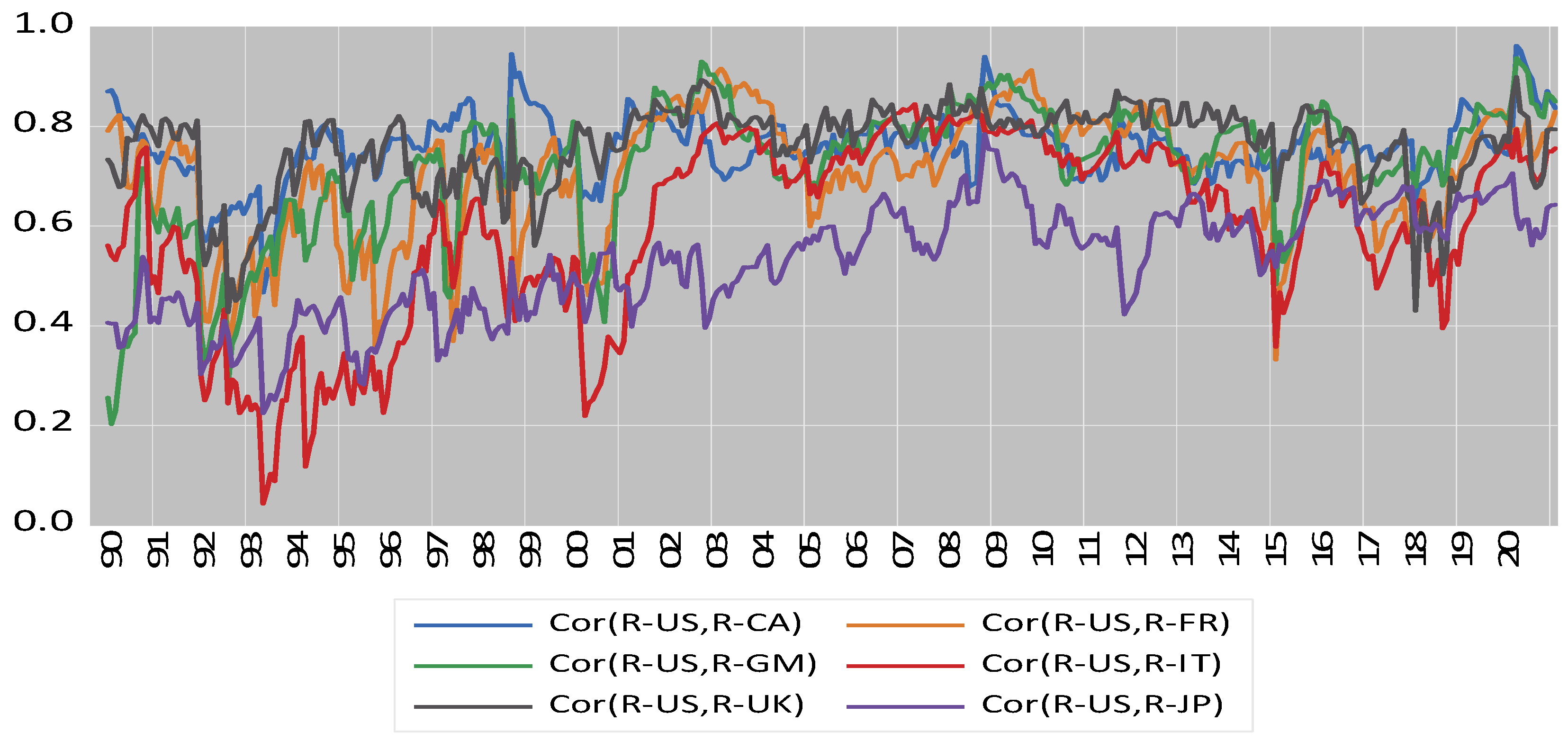
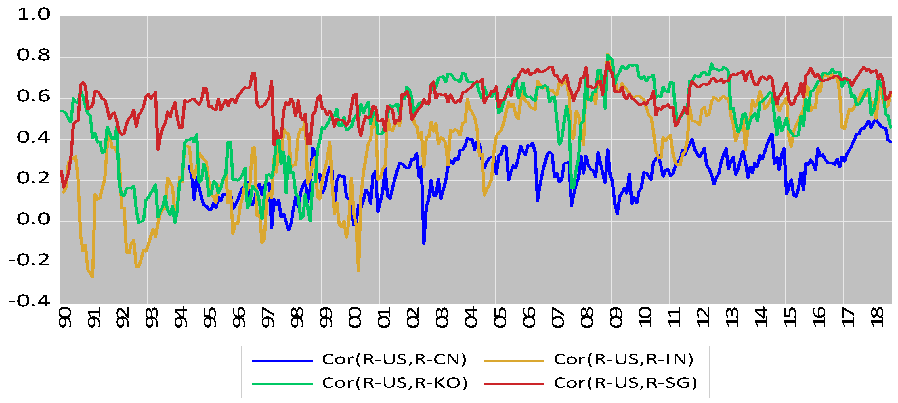
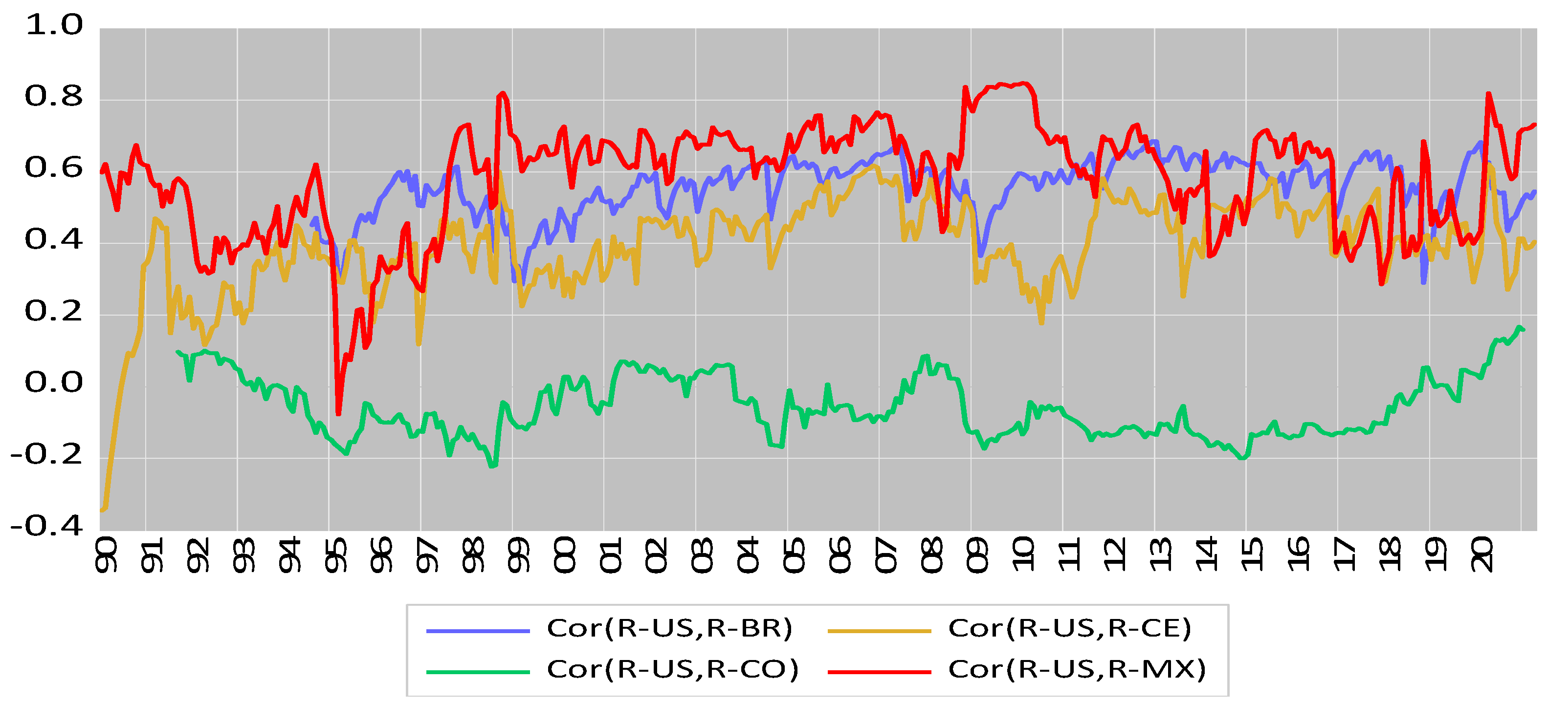
Figure 1, Figure 2 and Figure 3 present the time series plots of the dynamic correlation coefficients using a DCC model, as expressed in Equation (9). The vertical axis measures the estimated correlation coefficient, while the horizontal axis is year. Apparently, these correlation paths display time variations and exhibit some degree of comovements (except for the U.S.–Columbia pair); yet the correlation values diverge from market to market. These figures demonstrate that high correlations (except for the U.S.–Columbia pair) tend to cluster within different regions. More precise information is reported in Table 8, which shows the statistics for the correlation of coefficients between the U.S. and global market j, ,.
The statistics in Table 8 show the mean values of correlation coefficients across different markets vary from −0.0573 (Columbia) to 0.7616 (UK). The maximum values for the majority of markets, especially with Canada, lie between the period of April 2020 and May 2020, the peak period of COVID-19 spread. The minimum values are more diverse: some occur in the early 1990s, the U.S. dot.com collapse; others occur in 1997–1998 due to the impact of the Asia crisis. The values of standard deviations of the correlated coefficients vary from 0.0796 (Brazil) to 0.0650 (Canada). The evidence is consistent with the expectations of market participants.
Table 9 reports the correlations for the explanatory variable EPU between the U.S. and each global market. The estimated statistics indicate that correlations range from -0.04 (Columbia) to 0.75 (Canada and Singapore). In general, the major industrial countries display higher correlations of EPU with that of the U.S.
6.2. EPU and COVID-19 on Time-Varying Return Correlations
Longin and Solnik (1995) argued that the correlation between two asset market returns is linked to conditional variance. Connolly et al. (2005) found that the comovements of asset returns can be explained by the VIX. Chiang et al. (2016) reported that return correlation is linked to the conditional variance of national stock returns. To extend the above models, Equation (10) below is estimated using two country’s EPUs plus to explain the time-varying correlations of stock returns, and is expressed as:
in this section is the residual series obtained by regressing on , which avoids the impact of multicollinearity arising from the correlation between two EPU series. The , is the stock return correlation coefficient between the U.S. and an individual global market. A Fisher transformation applies, as the () series contains elements of negative values, that is, ,ln[ (Chiang et al. 2007).
Estimates for Equation (10), which was calculated twice, are reported in Table 10, which shows results for the pre-COVID-19 period from January 1993 to December 2018, and in Table 11, which contains results for the data extended to August 2021. The estimates in Table 10 show rather consistent results. It is evident that both and on the dynamic correlations are positive and statistically significant, indicating that the impact of policy uncertainty drives the two market returns in the same direction. Given the dominant position of the U.S. as a financial power in the global system (Rapach et al. 2013; Bhattarai et al. 2020; Chiang 2021), as well as the evidence from Table 2 and Table 3, the global transmission process can run through either , or , or both.
The impact of shows a similar effect, as indicated by the coefficients, which exhibit positive signs and are statistically significant in 11 out of the 14 markets. Obviously, the positive coefficients imply that two stock returns respond to in a similar fashion through the contagion effect stemming from news, media, or different types of electronic transmission (Jones et al. 2021). The transmitting process could run through ( (), as demonstrated in Table 6 and Table 7. the coefficients for Italy, China, and Columbia show opposite signs to those of the other markets. This could result from different market sensitivity or a relative low connection with the U.S., as shown in Table 8.
By extending the observations to August 2021, the time that experienced heightened periods of COVID-19, the estimated results are quite difference. The estimated results, which are reported in Table 11, show a large number of negative signs in the estimated parameters, including the group of G7 countries (expect Japan) for the coefficients on , the majority of countries in Asia and Latin America plus Canada for the coefficients of , and all countries except Canada, India, and Singapore13 for the coefficients of The negative coefficients reflect a decoupling of two market stock returns as uncertainty (, , and ) rises. The story behind these results is complex: a simple reason is that COVID-19 could non-synchronously hit different countries at different periods of time; investors in different countries may occasionally encounter different phases of COVID-19 shocks. This situation can be further distorted by the implementation of crisis rescue policies by different government regulations or the timing of different measures by different governments to control the virus spread. These events create different fears that can lead investors in different countries (Liu et al. 2021) to react to COVID-19 at varying speeds and with different levels of sensitivity (Davis et al. 2021). This study’s finding is consistent with the results reported by Zehri (2021), who found that the pandemic had less of an impact on stock prices and return volatilities in China than it did in the U.S. While comparing the estimated coefficients over the two tables, it is clear that the COVID-19 outbreak created significant instability on investments, as reflected in changes of signs in coefficients. This decoupling phenomenon differs from the return comovements that become stronger when volatility is high (Karolyi and Stulz 1996). However, the result is consistent with the evidence of structure change in stock return and volatility after COVID-19 spikes, as noted by Hong et al. (2021), Shahzad et al. (2021), and Wątorek et al. (2021). A follow-up question is this: when will the parameter stability in stock markets be restored, and how long will it take? This issue is left to future research.
7. Conclusions and Implications
This paper has several important findings. First, each country’s EPU has a negative effect on domestic stock returns; moreover, U.S. EPU presents a strong spillover effect that negatively affects global stock returns. However, no comparable findings of a significant negative effect run from the global markets to U.S. stocks, with the exception of France and Germany.
Second, testing the model using a differenced form shows changes in both domestic EPU and U.S. EPU, which exhibits a similar performance. That is, a heightened EPU has a negative effect on domestic stock market returns, and an upshift of U.S. EPU also produces a spillover effect in the global stock markets, with the exception of the Columbian market. This study suggests that using to explain stock returns is a more appropriate approach, since an estimated negative coefficient of this variable would reflect a negative effect on the stock returns in the current period, but a positive coefficient in the lagged term indicates the presence of a risk premium for investors who bought stocks during a period of heightened uncertainty.
Third, this study finds evidence of negative coefficients for , which is used as a proxy for the uncertainty of COVID-19. The significance of this variable shows the directly damaging effect of COVID-19 on global stock returns. This finding is consistent with the existing literature using an event study methodology to examine the impact of COVID-19 on stock returns (Yan 2020; Lee et al. 2020; Hung et al. 2021; Khatatbeh et al. 2020).
Fourth, the impact of COVID-19 on stock returns also carries an indirect effect via its influence on stock market volatility. The interactive effect is negative and statistically significant for 11 out of 14 countries. This finding suggests that the model is nonlinear and also implies that the market is inefficient. Apparently, the exclusion of this nonlinear term could lead to biased estimates.
Fifth, this study demonstrates that U.S. EPU, global EPU, and infectious induced volatility play vital roles in the explanation of stock return comovement. During a tranquil period, these uncertainty measures have positive and relative stable comovement on stock returns. However, during a time of volatility, such as the COVID-19 pandemic, the pairwise correlation coefficients exhibit a V-shape path as noted by Chiang et al. (2007). In the short run, and in the early stage of the pandemic, the two country’s stock returns exhibit a negative correlation; however, at a later stage, the stock returns merge, and the correlation turns positive (Chiang et al. 2007; Davis et al. 2021). Evidence from this study on dynamic conditional correlation confirms the first stage phenomenon in the literature.
This study has several policy implications. First, the impact of COVID-19 has more profound effects on stock returns than a single factor measure. This study demonstrates that, in addition to the direct effect, there is an indirect effect that enhances the adverse effect on stock returns. As a result, policymakers should pay particular attention to a broader dimension of uncertainly that captures the impacts of infectious disease on economic structures, expectations, and the stock market volatility of stock market prices. Second, this study finds that COVID-19 affects the stock returns of different countries to a different degree. Heightened infectious disease volatility tends to produce stock return divergence between each global market and the U.S. market. The decoupling of pairwise return phenomenon also would create some sort of short-term speculative profits through arbitraging activities in global stock markets. This can further exacerbate stock market instability. This information can be useful to policymakers as they seek to design more effective policies to stabilize capital markets in the early stage of the virus’ spread.
From an academic point of view, this study also has some implications. Specifically, this analysis can also apply to other categorical policy uncertainty via a replacement of EPU by geopolitical risk (GRP) or monetary policy uncertainty (MPU) if the data are available. Further, the analysis can be extended to other pairs of asset returns such as gold returns and stock returns (Bouoiyour et al. 2018) and the dynamic relationship between real exchange rates and stock return differentials (Moore and Wang 2014). Those issues go beyond the scope of this current study and deserve an independent paper.
Funding
This research received no external funding.
Data Availability Statement
The stock index data and dividend yields were downloaded from the Datastream subscripted by Drexel University. The economic policy uncertainty data and equity market volatility data were obtained from the website of Economic Policy Uncertainty (Baker et al. 2016; Davis 2016, both data were updated on a monthly basis. All the data mentioned above except the dividend yields can be obtained freely from the Federal Reserve Bank at St. Louise. economic data base.
Conflicts of Interest
The authors declare no conflict of interest.
Appendix A. Estimating the Time-Varying Correlations
Engle (2002) proposes a dynamic conditional correlation model applicable to estimating time-varying correlations of two stock market returns. Similar types of empirical estimations have been conducted by Chiang et al. (2007) and Kenourgios et al. (2011). This model is appealing because of its ability to deal with a vector of return correlations and to handle a volatility clustering phenomenon. Further, it can alleviate the heteroscedasticity problem (Forbes and Rigobon 2002). Let {Rt} denote a vector of bivariate return series, which is expressed as:
where Rt = is a 2 × 1 vector for stock market returns, is the mean value of stock i or j, which has the conditional expectation of multivariate time series properties14, and the error vector where is the information set up for (and including) time t − 1.
In the multivariate DCC–GARCH structure, the conditional variance–covariance matrix is assumed to be:
where = diag is the diagonal matrix of time-varying standard deviations from univariate models, and Pt is the time-varying conditional correlation matrix, which satisfies the following conditions:
where is a correlation matrix with ones on the diagonal and off-diagonal elements that have an absolute value less than unity (Engle 2002). To capture a dynamic adjustment of correlation, one must have a negative shock, which differs from that for a positive shock, and Engle (2009) proposed an asymmetric DCC (ADCC) model, expressed as:
where the is positive definite and .
The product of will be nonzero. Thus, a positive value of indicates that correlations increase more in response to market falls than they do to market rises. The equation is written as:
where = is assumed to be the 2 × 2 time-varying covariance matrix of , = E which is a 2 × 2 unconditional variance matrix of (where ), is the 2 × 2 unconditional variance matrix of ; ,are non-negative scalar parameters. Substituting Equation (A5) for (A4) yields:
where is the dynamic correlation coefficient between stock return i and j. is the stochastic matrix that delivers a positive definite, quasi-correlation matrix between stock returns i and j for time t. The Equation (A6) can be used to derive the time-varying correlations for the stock returns i and j. The ADCC model can be estimated by employing a two-stage approach to maximize the log-likelihood function (Engle 2009).
| 1 | |
| 2 | Knight differentiated risk from uncertainty by the measurability vs. immeasurability. Knight (1921) defined only quantifiable uncertainty to be risk. However, the EPU indices provided by Baker et al. (2016) help to quantify the measurability of uncertainty. |
| 3 | Hillen et al. (2017) emphasize the concept that uncertainty provokes fear and perceptions of vulnerability. |
| 4 | Global indices are from: http://www.policyuncertainty.com/media/Global_Annotated_Series.pdf (accessed on 6 June 2021). |
| 5 | Baker et al. (2020a) use the following terms (term variants): E: {economic, economy, financial}; M: {“stock market”, equity, equities, “Standard and Poors”}; V: {volatility, volatile, uncertain, uncertainty, risk, risky};ID:{epidemic, pandemic, virus, flu, disease, coronavirus, mers, sars, ebola, H5N1, H1N1}. |
| 6 | A model that incorporates an asymmetry shock (Nelson 1991) is not considered, since this information will be captured by a lag of the COVID disease shock at a later point. The use of GARCH (1,1) was popularized by Bollerslev et al. (1992) as a way to achieve a better fit of the stock return equation. Bollerslev (2010) provides a summary of different specification of GARCH-type models. |
| 7 | A kurtosis above 3 indicates “fat tails,” or leptokurtosis, relative to the normal, or Gaussian, distribution. Platykurtosis refers to a distribution that has a negative excess kurtosis with a relatively flatter peak than a normal distribution. |
| 8 | Bollerslev (2010) provides alternative specifications of the GARCH-type model. |
| 9 | As arrival of COVID-19 in U.S. on early 2020, the Dow Jones Industrial Average (DJIA) was down 3.56%, S&P 500 decreased 3.35%, and NASDAQ dropped 3.71%. Recently, as COVID-19 variant emerged from news, the DJIA fell 2.53%, while the S&P 500 and NASDAQ Composite declined 2.27% and 2.23%, respectively. causing a big sell-off on Friday, November 26. Specifically, Futures on the DJIA dropped 415 points or 1.18% S&P 500 futures were down 0.78%, and Nasdaq 100 futures fell 0.4% as reported by Yun Li for CNBC on November 30, 2021, 03:30 AM EST. |
| 10 | IMF provides a report with respect to various key policy responses for different countries (See Policy response to COVID-19–International Monetary Fund, www.imf.org (accessed on 6 June 2021)). |
| 11 | + + + + . |
| 12 | |
| 13 | Canada, India and Singapore are thought much heighted connected with U.S., both on the economic and political aspects, that renders a positive respond to the The same argument apply to Japan for the coefficient of |
| 14 | Some researcers alternatively use a factor model by specifying size and value factors and other style factors as exogenous variables in their mean equation. |
References
- Antonakakis, Nikolaos, Ioannis Chatziantoniou, and George Filis. 2013. Dynamic co-movements of stock market returns, implied volatility and policy uncertainty. Economics Letters 120: 87–92. [Google Scholar] [CrossRef]
- Arouri, Mohamed, Christophe Estay, Christophe Rault, and David Roubaud. 2016. Economic policy uncertainty and stock markets: Long run evidence from the US. Finance Research Letters 18: 136–41. [Google Scholar] [CrossRef]
- Bahrini, Raéf, and Assaf Filfilan. 2020. Impact of the novel coronavirus on stock market returns: Evidence from GCC countries. Quantitative Finance and Economics 4: 640–52. [Google Scholar] [CrossRef]
- Baker, Scott R., Nicholas Bloom, and Steven J. Davis. 2016. Measuring economic policy uncertainty. Quarterly Journal of Economics 131: 1593–636. [Google Scholar] [CrossRef]
- Baker, Scott R., Nicholas Bloom, Steven J. Davis, and Kyle Kost. 2019. Policy News and Stock Market Volatility. Available online: https://www.policyuncertainty.com/media/Policy%20News%20and%20Stock%20Market%20Volatility.pdf (accessed on 12 October 2021).
- Baker, Scott R., Nicholas Bloom, Steven J. Davis, and Stephen J. Terry. 2020a. COVID-Induced Economic Uncertainty. NBER Working Paper No. 26983. Cambridge: National Bureau of Economic Research. [Google Scholar]
- Baker, Scott R., Nicholas Bloom, Steven J. Davis, Kyle Kost, Marco Sammon, and Tasaneeya Viratyosin. 2020b. The Unprecedented stock market reaction to COVID-19. The Review of Asset Pricing Studies 10: 742–58. [Google Scholar] [CrossRef]
- Bhattarai, Saroj, Arpita Chatterjee, and Woong Yong Park. 2020. Global spillover effects of US uncertainty. Journal of Monetary Economics 114: 71–89. [Google Scholar] [CrossRef] [Green Version]
- Bloom, Nicholas. 2009. The impact of uncertainty shocks. Econometrica 77: 623–685. [Google Scholar]
- Bloom, Nicholas. 2014. Fluctuations in Uncertainty. Journal of Economic Perspectives 28: 153–76. [Google Scholar] [CrossRef] [Green Version]
- Bollerslev, Tim. 2010. Glossary to ARCH (GARCH) in Volatility and Time Series Econometrics: Essays in Honor of Robert Engle. Edited by Tim Bollerslev, Jeffrey Russell and Mark Watson. Oxford: Oxford University Press. [Google Scholar]
- Bollerslev, Tim, Ray Y. Chou, and Kenneth F. Kroner. 1992. ARCH modeling in finance: A review of the theory and empirical evidence. Journal of Econometrics 52: 5–59. [Google Scholar] [CrossRef]
- Bora, Debakshi, and Daisy Basistha. 2021. The outbreak of COVID-19 and its impact on stock market volatility: Evidence from a worst affected economy. Journal of Public Affairs 2021: e2623. [Google Scholar] [CrossRef]
- Bouoiyour, Jamal, Refk Selmi, and Mark E. Wohar. 2018. Measuring the response of gold prices to uncertainty: An analysis beyond the mean. Economic Modeling 75: 1–12. [Google Scholar] [CrossRef] [Green Version]
- Brogaard, Jonathan, and Andrew Detzel. 2015. The Asset Pricing Implications of Government Economic Policy Uncertainty. Management Science 61: 3–18. [Google Scholar] [CrossRef] [Green Version]
- Caggiano, Giovanni, Efrem Castelnuovo, and Nicolas Groshenny. 2014. Uncertainty shocks and unemployment dynamics in U.S. recessions. Journal of Monetary Economics 67: 78–92. [Google Scholar] [CrossRef] [Green Version]
- Chatjuthamard, Pattanaporn, Pavitra Jindahra, Pattarake Sarajoti, and Sirimon Treepongkaruna. 2021. The effect of COVIC-19 on the global stock market. Accounting & Finance 61: 4923–53. [Google Scholar]
- Chatziantoniou, Ioannis, David Duffy, and George Filis. 2013. Stock market response to monetary and fiscal policy shocks: Multi-country evidence. Economic Modelling 30: 754–69. [Google Scholar] [CrossRef] [Green Version]
- Chen, Cathy W. S., Thomas C. Chiang, and Mike K. P. So. 2003. Asymmetrical reaction to US stock-return news: Evidence from major stock markets based on a double-threshold model. Journal of Economics and Business 55: 487–502. [Google Scholar] [CrossRef]
- Chen, Cathy Yi-Hsuan, and Thomas C. Chiang. 2016. Empirical analysis of the intertemporal relation between downside risk and expected returns: Evidence from time-varying transition probability models. European Financial Management 22: 749–96. [Google Scholar] [CrossRef]
- Chen, Cathy Yi-Hsuan, Thomas C. Chiang, and Wolfgang Karl Härdle. 2018. Downside risk and stock returns in the G7 countries: An empirical analysis of their long-run and short-run dynamics. Journal of Banking & Finance 93: 21–32. [Google Scholar]
- Chen, Jian, Fuwei Jiang, and Guoshi Tong. 2017. Economic policy uncertainty in China and stock market expected returns. Accounting & Finance 57: 1265–86. [Google Scholar]
- Chiang, Thomas C. 2019. Economic policy uncertainty, risk and stock returns: Evidence from G7 stock markets. Finance Research Letters 29: 41–49. [Google Scholar] [CrossRef]
- Chiang, Thomas C. 2020. US policy uncertainty and stock returns: Evidence in the US and its spillovers to European Union, China, and Japan. Journal of Risk Finance 21: 621–57. [Google Scholar] [CrossRef]
- Chiang, Thomas C. 2021. Spillovers of U.S. market volatility and monetary policy uncertainty to global stock markets. North American Journal of Economics and Finance 58: 474–501. [Google Scholar] [CrossRef]
- Chiang, Thomas C., Bang Nam Jeon, and Huimin Li. 2007. Dynamic correlation analysis of financial contagion: Evidence from Asian markets. Journal of International Money and Finance 26: 1206–28. [Google Scholar] [CrossRef]
- Chiang, Thomas C., Lanjun Lao, and Qingfeng Xue. 2016. Comovements between Chinese and global stock markets: Evidence from aggregate and sectoral data. Review of Quantitative Finance and Accounting 47: 1003–42. [Google Scholar] [CrossRef]
- Chiang, Thomas C., and Yuanqing Zhang. 2018. An Empirical Investigation of Risk-Return Relations in Chinese Equity Markets: Evidence from Aggregate and Sectoral Data. International Journal of Financial Studies 6: 35. [Google Scholar] [CrossRef] [Green Version]
- Christou, Christina, Juncal Cunado, Rangan Gupta, and Christis Hassapis. 2017. Economic policy uncertainty and stock market returns in Pacific-Rim countries: Evidence based on a Bayesian panel VAR model. Journal of Multinational Financial Management 40: 92–102. [Google Scholar] [CrossRef]
- Connolly, Robert, Chris Stivers, and Licheng Sun. 2005. Stock market uncertainty and the stock-bond return relation. Journal of Financial and Quantitative Analysis 40: 161–94. [Google Scholar] [CrossRef] [Green Version]
- Davis, Steven. 2016. An Index of Global Economic Policy Uncertainty. NBER Working Paper 22740. Available online: https://ideas.repec.org/p/nbr/nberwo/22740.html (accessed on 1 October 2021).
- Davis, Steven J., Dingqian Liu, and Xuguang Simon Sheng. 2021. Stock prices and economic activity in the time of coronavirus. IMF Economic Review. [Google Scholar] [CrossRef]
- Ding, Zhuanxin, Clive W. J. Granger, and Robert F. Engle. 1993. A long memory property of stock market returns and a new model. Journal of Empirical Finance 1: 83–106. [Google Scholar] [CrossRef]
- Engle, Robert F. 2002. Dynamic conditional correlation: A simple class of multivariate generalized autoregressive conditional heteroskedasticity models. Journal of Business and Economic Statistics 20: 339–50. [Google Scholar] [CrossRef]
- Engle, Robert F. 2009. Anticipating Correlations: A New Paradigm for Risk Management. Princeton: Princeton University Press. [Google Scholar]
- Forbes, Kristin J., and Roberto Rigobon. 2002. No contagion, only Interdependence: Measuring stock market co-movements. Journal of Finance 57: 2223–62. [Google Scholar] [CrossRef]
- French, Kenneth R., G. William Schwert, and Robert F. Stambaugh. 1987. Expected stock returns and volatility. Journal of Financial Economics 19: 3–29. [Google Scholar] [CrossRef] [Green Version]
- Guo, Hui, and Robert F. Whitelaw. 2006. Uncovering the risk-return relation in the stock market. Journal of Finance 61: 1433–63. [Google Scholar] [CrossRef] [Green Version]
- Hillen, Marij A., Caitlin M. Gutheil, Tania D. Strout, Ellen M. A. Smets, and Paul K. J. Han. 2017. Tolerance of uncertainty: Conceptual analysis, integrative model, and implications for healthcare. Social Science & Medicine 180: 62–75. [Google Scholar]
- Hong, Hui, Zhicun Bian, and Chien-Chiang Lee. 2021. COVID-19 and instability of stock market performance: Evidence from the U.S. Financial Innovation 7: 12. [Google Scholar] [CrossRef]
- Hung, Dao Van, Nguyen Thi Minh Hue, and Vu Thuy Duong. 2021. The impact of COVID-19 on stock market returns in Vietnam. Journal of Risk Financial Management 14: 441. [Google Scholar] [CrossRef]
- Indrayono, Yohanes. 2021. What factors affect stocks’ abnormal return during the COVID-19 pandemic: Data from the Indonesia stock exchange. European Journal of Business & Management Research 6: 1–11. [Google Scholar] [CrossRef]
- Jones, Lora, Daniele Palumbo, and David Brown. 2021. Coronavirus: How the pandemic has changed the world economy. BBC News. March 4. Available online: www.bbc.com (accessed on 30 November 2021).
- Karolyi, G. Andrew, and René M. Stulz. 1996. Why do markets move together? An investigation of US-Japanese stock return comovements. Journal of Finance 51: 951–86. [Google Scholar] [CrossRef]
- Kenourgios, Dimitris, Aristeidis Samitas, and Nikos Paltalidis. 2011. Financial crises and stock market contagion in a multivariate time-varying asymmetric framework. Journal of International Financial Markets, Institutions and Money 21: 92–106. [Google Scholar] [CrossRef]
- Khatatbeh, Ibrahim N., Mohammad Bani Hani, and Mohammed N. Abu-Alfoul. 2020. The impact of COVID-19 pandemic on global stock markets: An event study. International Journal of Economics and Business Administration 8: 505–14. [Google Scholar] [CrossRef]
- Knight, Frank H. 1921. Risk, Uncertainty, and Profit, 5th ed. New York: Dover Publications. [Google Scholar]
- Latif, Yousaf, Ge Shunqi, Shahid Bashir, Wasim Iqbal, Salman Ali, and Muhammad Ramzan. 2021. COVID-19 and stock exchange return variation: Empirical evidence from econometric estimation. Environmental Science and Pollution Research 28: 60019–31. [Google Scholar] [CrossRef] [PubMed]
- Lee, Kelvin Yong-Ming, Mohamad Jais, and Chia-Wen Chan. 2020. Impact of Covid-19: Evidence from Malaysian stock market. International Journal of Business and Society 21: 607–28. [Google Scholar]
- Li, Qi, Jian Yang, Cheng Hsiao, and Young-Jae Chang. 2005. The relationship between stock returns and volatility in international stock markets. Journal of Empirical Finance 12: 650–65. [Google Scholar] [CrossRef]
- Li, Xiao-Ming. 2017. New evidence on economic policy uncertainty and equity premium. Pacific-Basin Finance Journal 46: 41–56. [Google Scholar] [CrossRef]
- Liow, Kim Hiang, Wen-Chi Liao, and Yuting Huang. 2018. Dynamics of international spillovers and interaction: Evidence from financial market stress and economic policy uncertainty. Economic Modelling 68: 96–116. [Google Scholar] [CrossRef]
- Liu, Li, and Tao Zhang. 2015. Economic policy uncertainty and stock market volatility. Finance Research Letter 15: 99–105. [Google Scholar] [CrossRef] [Green Version]
- Liu, Zhifeng, Toan Luu Duc Huynh, and Peng-Fei Dai. 2021. The impact of COVID-19 on the stock market crash risk in China. Research in International Business and Finance 57: 101419. [Google Scholar] [CrossRef]
- Longin, Francois, and Bruno Solnik. 1995. Is the correlation in international equity returns constant: 1960–1990? Journal of International Money and Finance 14: 3–26. [Google Scholar] [CrossRef]
- Menzly, Lior, Tano Santos, and Pietro Veronesi. 2004. Understanding predictability. Journal of Political Economy 112: 1–47. [Google Scholar] [CrossRef] [Green Version]
- Merton, Robert C. 1973. An intertemporal capital asset pricing model. Econometrica 41: 867–87. [Google Scholar] [CrossRef]
- Merton, Robert C. 1980. On estimating the expected return on the market: An exploratory investigation. Journal of Financial Economics 8: 323–61. [Google Scholar] [CrossRef]
- Moore, Tomoe, and Ping Wang. 2014. Dynamic linkage between real exchange rates and stock prices: Evidence from developed and emerging Asian markets. International Review of Economics & Finance 29: 1–11. [Google Scholar]
- Mugiarni, Ajeng, and Permata Wulandari. 2021. The Effect of Covid-19 Pandemic on Stock Returns: An evidence of Indonesia stock exchange. Journal of International Conference Proceedings 4: 28–37. [Google Scholar] [CrossRef]
- Nelson, Daniel B. 1991. Conditional heteroskedasticity in asset returns: A new approach. Econometrica 59: 347–370. [Google Scholar] [CrossRef]
- Nian, Rui, Yijin Xu, Qiang Yuan, Chen Feng, and Amaury Lendasse. 2021. Quantifying time-frequency co-movement impact of COVID-19 on U.S. and China stock market toward investor sentiment index. Frontiers in Public Health 9: 727047. [Google Scholar] [CrossRef] [PubMed]
- Ozoguz, Arzu. 2009. Good times or bad times? Investors’ uncertainty and stock returns. Review of Financial Studies 22: 4377–422. [Google Scholar] [CrossRef]
- Rapach, David E., Jack K. Strauss, and Guofu Zhou. 2013. International stock return predictability: What is the role of the United States? Journal of Finance 68: 1633–22. [Google Scholar] [CrossRef]
- Rubbaniy, Ghulame, Ali Awais Khalid, Muhammad Umar, and Nawazish Mirza. 2021. European Stock Markets’ Response to COVID-19, Lockdowns, Government Response Stringency and Central Banks’ Interventions. Available online: https://ssrn.com/abstract=3785598 (accessed on 8 December 2021).
- Shahzad, Syed Jawad Hussain, Elie Bouri, Ladislav Kristoufek, and Tareq Saeed. 2021. Impact of the COVID-19 outbreak on the US equity sectors: Evidence from quantile return spillovers. Financial Innovation 7: 1–23. [Google Scholar] [CrossRef]
- Singh, Gurmeet, and Muneer Shaik. 2021. The short-term impact of COVID-19 on global stock market indices. Contemporary Economics 15: 1–18. [Google Scholar] [CrossRef]
- Trung, Nguyen Ba. 2019. The Spillover Effect of the US Uncertainty on Emerging Economies: A panel VAR approach. Applied Economics Letters 26: 210–16. [Google Scholar] [CrossRef]
- Wątorek, Marcin, Jarosław Kwapień, and Stanisław Drożdż. 2021. Financial return distributions: Past, present, and COVID-19. Entropy 23: 884. [Google Scholar] [CrossRef]
- Yan, Chao. 2020. COVID-19 outbreak and stock prices: Evidence from China. SSRN 3574374. Available online: https://ssrn.com/abstract=3574374 (accessed on 1 October 2021).
- Youssef, Manel, Khaled Mokni, and Ahdi Noomen Ajmi. 2021. Dynamic connectedness between stock markets in the presence of the COVID-19 pandemic: Does economic policy uncertainty matter? Financial Innovation 7: 13. [Google Scholar] [CrossRef]
- Zehri, Chokri. 2021. Stock market comovements: Evidence from the COVID-19 pandemic. The Journal of Economic Asymmetries 24: e00228. [Google Scholar] [CrossRef] [PubMed]
Figure 1.
Plots of dynamic correlation coefficients for U.S. and other G7 markets.

Figure 2.
Plots of dynamic correlation coefficients for U.S. and major Asia markets.

Figure 3.
Plots of dynamic correlation coefficients for U.S. and Latin America markets.


Table 1.
Regression estimates of the national stock return on domestic EPU(i) using the GED–GARCH procedure.
Table 1.
Regression estimates of the national stock return on domestic EPU(i) using the GED–GARCH procedure.
| Market | C | ||||||
|---|---|---|---|---|---|---|---|
| Panel A | 9.2456 | −1.7804 | 2.6838 | 0.9218 | 0.7993 | 0.021 | |
| 43.49 | −48.97 | 0.42 | 1.02 | 4.19 | |||
| 3.4020 | −0.6431 | 1.0573 | 0.5141 | 0.7975 | 0.024 | ||
| 17.20 | −14.66 | 0.52 | 0.95 | 3.73 | |||
| 1.3583 | −0.2260 | 2.2151 | 0.5312 | 0.7394 | 0.004 | ||
| 13.55 | −9.22 | 0.60 | 0.81 | 2.46 | |||
| 3.8502 | −0.7652 | 1.6395 | 0.5014 | 0.7888 | 0.020 | ||
| 7.00 | −6.68 | 0.60 | 0.81 | 3.54 | |||
| 3.5922 | −0.7206 | 1.5669 | 0.4706 | 0.8151 | 0.007 | ||
| 8.26 | −8.04 | 0.41 | 0.81 | 3.58 | |||
| 2.0566 | −0.3813 | 2.2151 | 0.5564 | 0.6991 | 0.007 | ||
| 9.66 | −9.59 | 0.60 | 0.78 | 1.91 | |||
| 3.9755 | −0.8276 | 0.0511 | 0.3896 | 0.8899 | 0.007 | ||
| 58.64 | −68.16 | 0.10 | 1.10 | 9.10 | |||
| Panel B | 2.8454 | −0.5234 | 5.8669 | 0.3606 | 0.7421 | 0.005 | |
| 24.65 | −13.54 | 0.73 | 0.70 | 2.78 | |||
| 7.3318 | −1.5870 | 7.4521 | 0.3243 | 0.6930 | 0.066 | ||
| 11.41 | −10.98 | 0.42 | 0.45 | 1.08 | |||
| 1.7588 | −0.3586 | 1.4725 | 0.5531 | 0.8223 | 0.002 | ||
| 7.02 | −7.73 | 0.51 | 1.07 | 5.39 | |||
| 5.7930 | −1.1537 | 1.8871 | 0.7118 | 0.6663 | 0.037 | ||
| 13.47 | −13.04 | 0.67 | 0.89 | 2.01 | |||
| Panel C | 2.0072 | −0.3629 | 36.6671 | 1.1989 | 0.0902 | 0.006 | |
| 22.85 | −10.82 | 1.55 | 1.04 | 0.26 | |||
| 5.6974 | −1.1701 | 1.4079 | 0.1244 | 0.7470 | 0.034 | ||
| 5.34 | −5.01 | 0.79 | 1.02 | 2.97 | |||
| 0.6241 | −0.1306 | 1.6867 | 0.2400 | 0.8058 | 0.003 | ||
| 4.09 | −3.90 | 0.57 | 1.01 | 3.81 | |||
| 1.3676 | −0.2215 | 3.2422 | 0.4435 | 0.7712 | 0.002 | ||
| 6.57 | −4.22 | 0.55 | 0.66 | 2.53 |
Notes: The dependent variable is national stock returns, ; the independent variable is national economic policy uncertainty, . The model is estimated by using the GED–GARCH(1,1) process. Numbers in the first row are the estimated coefficients, the second row shows the t-statistics. The critical values of t-distribution at the 1%, 5%, and 10% levels of significance are 2.63, 1.98, and 1.66, respectively.
Table 2.
Estimates of the global stock returns in response to U.S. economic policy uncertainty using the GED–GARCH procedure.
Table 2.
Estimates of the global stock returns in response to U.S. economic policy uncertainty using the GED–GARCH procedure.
| Market | C | ||||||
|---|---|---|---|---|---|---|---|
| Panel A | 6.4605 | −1.3264 | 0.8016 | 0.5987 | 0.7981 | 0.040 | |
| 57.44 | −47.31 | 0.47 | 1.01 | 4.18 | |||
| 5.9379 | −1.2225 | 1.2473 | 0.5324 | 0.7963 | 0.030 | ||
| 17.59 | −16.43 | 0.52 | 0.88 | 3.60 | |||
| 6.2713 | −1.2989 | 1.8783 | 0.5175 | 0.7660 | 0.032 | ||
| 12.56 | −12.08 | 0.65 | 0.90 | 3.43 | |||
| 6.3616 | −1.3085 | 1.7092 | 0.5683 | 0.8006 | 0.023 | ||
| 19.95 | −19.06 | 0.49 | 0.89 | 3.77 | |||
| 6.2653 | −1.3144 | 1.2556 | 0.5127 | 0.7665 | 0.040 | ||
| 27.52 | −28.94 | 0.55 | 0.82 | 2.88 | |||
| 3.9773 | −0.8238 | 0.0081 | 0.3093 | 0.9167 | 0.011 | ||
| 49.59 | −56.61 | 0.02 | 0.96 | 10.52 | |||
| Panel B | 9.6793 | −2.0053 | 3.0395 | 0.2010 | 0.8253 | 0.027 | |
| 26.58 | −25.54 | 0.97 | 0.79 | 5.92 | |||
| 5.0161 | −1.0040 | 4.2392 | 0.3231 | 0.8167 | 0.007 | ||
| 6.62 | −6.04 | 0.63 | 0.86 | 3.98 | |||
| 2.3167 | −0.4624 | 4.1761 | 1.0240 | 0.7989 | 0.001 | ||
| 3.08 | −2.89 | 0.52 | 0.85 | 3.79 | |||
| 3.1397 | −0.6311 | 1.4576 | 0.6254 | 0.7357 | 0.012 | ||
| 16.81 | −14.19 | 0.84 | 1.29 | 4.46 | |||
| Panel C | 8.0327 | −1.6380 | 23.6677 | 0.9735 | 0.0763 | 0.020 | |
| 11.35 | −10.04 | 1.98 | 1.38 | 0.32 | |||
| 2.5995 | −0.4680 | 4.7147 | 0.2519 | 0.6236 | 0.003 | ||
| 5.13 | −3.96 | 0.58 | 0.74 | 1.18 | |||
| 3.9392 | −0.7955 | 2.7380 | 0.2189 | 0.7791 | 0.008 | ||
| 14.20 | −17.37 | 0.60 | 0.84 | 2.92 | |||
| 6.7019 | −1.2737 | 1.2727 | 0.1398 | 0.8808 | 0.005 | ||
| 23.06 | −21.50 | 0.65 | 0.89 | 6.81 |
Notes: The dependent variable is national stock returns, ; the independent variable is U.S. economic policy uncertainty, The model is estimated by using the GED–GARCH(1,1) process. Numbers in the first row are the estimated coefficients, the second row shows the t-statistics. The critical values of t-distribution at the 1%, 5%, and 10% levels of significance are 2.63, 1.98, and 1.66, respectively.
Table 3.
U.S stock return in response to each global economic policy uncertainty.
| US Return | C | ||||||
|---|---|---|---|---|---|---|---|
| Panel A | 1.4823 | −0.0410 | 1.7913 | 0.4462 | 0.7776 | −0.014 | |
| 2.08 | −0.28 | 0.71 | 1.30 | 4.92 | |||
| 1.3583 | −0.2260 | 2.2151 | 0.5312 | 0.7394 | 0.004 | ||
| 13.55 | −9.22 | 0.60 | 0.81 | 2.46 | |||
| 3.8502 | −0.7652 | 1.6395 | 0.5014 | 0.7888 | 0.020 | ||
| 7.00 | −6.68 | 0.60 | 0.81 | 3.54 | |||
| 0.9425 | −0.0016 | 0.8612 | 0.2214 | 0.7576 | −0.005 | ||
| 0.32 | −0.00 | 1.60 | 3.34 | 11.56 | |||
| 2.0944 | −0.1447 | 1.5580 | 0.3939 | 0.7585 | −0.022 | ||
| 3.88 | −1.30 | 0.82 | 1.47 | 5.09 | |||
| 2.5850 | −0.2717 | 1.2028 | 0.3072 | 0.7937 | −0.013 | ||
| 1.37 | −0.65 | 0.78 | 1.44 | 6.05 | |||
| Panel B | 1.3617 | 0.0137 | 1.3341 | 0.3512 | 0.7839 | −0.024 | |
| 2.95 | 0.12 | 0.78 | 1.30 | 5.59 | |||
| −1.0616 | 0.6082 | 1.5865 | 0.3688 | 0.7283 | −0.069 | ||
| −1.50 | 3.92 | 0.76 | 1.29 | 3.90 | |||
| 2.1825 | −0.1852 | 1.0027 | 0.2614 | 0.7718 | −0.013 | ||
| 1.99 | −0.76 | 1.04 | 1.86 | 6.97 | |||
| 3.2477 | −0.4153 | 1.2270 | 0.2543 | 0.7457 | −0.012 | ||
| 1.96 | −1.17 | 0.83 | 1.51 | 4.55 | |||
| Panel C | 1.7224 | −0.0890 | 1.8999 | 0.4008 | 0.7283 | −0.012 | |
| 4.50 | −1.05 | 0.87 | 1.43 | 4.16 | |||
| 3.5865 | −0.4809 | 1.1412 | 0.2811 | 0.7581 | −0.012 | ||
| 2.57 | −1.54 | 1.11 | 1.78 | 6.35 | |||
| 1.2896 | 0.0484 | 2.1000 | 0.4208 | 0.7244 | −0.032 | ||
| 16.11 | 4.59 | 0.77 | 1.29 | 3.80 | |||
| 2.0597 | −0.1390 | 1.4469 | 0.4134 | 0.7528 | −0.028 | ||
| 3.73 | −1.19 | 0.85 | 1.41 | 5.04 |
Notes: The dependent variable is U.S. stock returns, ; the independent variable is each global market’s economic policy uncertainty, . The model is estimated by using the GED–GARCH(1,1) process. Numbers in the first row are the estimated coefficients, the second row shows the t-statistics. The critical values of t-distribution at the 1%, 5%, and 10% levels of significance are 2.63, 1.98, and 1.66, respectively. U.S. market return only responds negatively to the EPU in FR and GM and is statistically significant.
Table 4.
Estimates of the global stock returns in response to change in economic policy uncertainty, change in infected decease uncertainty, and dividend yield using the GED–GARCH procedure.
Table 4.
Estimates of the global stock returns in response to change in economic policy uncertainty, change in infected decease uncertainty, and dividend yield using the GED–GARCH procedure.
| Market | C | |||||||
|---|---|---|---|---|---|---|---|---|
| Panel A: World and G7 markets | ||||||||
| 0.1096 | −0.0823 | −0.0028 | 1.3127 | 15.9656 | 1.2466 | 0.6377 | 0.11 | |
| 0.63 | −21.24 | −5.87 | 5.79 | 0.50 | 0.73 | 1.65 | ||
| −0.0839 | −0.0484 | −0.0021 | 1.5487 | 4.7491 | 0.7632 | 0.7438 | 0.05 | |
| −6.18 | −14.19 | −3.33 | 25.89 | 0.58 | 1.04 | 3.04 | ||
| 0.7429 | −0.0280 | −0.0064 | 0.0416 | 5.8430 | 0.6865 | 0.8821 | 0.05 | |
| 18.75 | −28.69 | −16.71 | 5.45 | 0.41 | 0.73 | 5.21 | ||
| 0.9777 | −0.0173 | −0.0007 | 0.5220 | 13.6361 | 1.2435 | 0.6199 | 0.01 | |
| 3.00 | −12.45 | −7.00 | 1.94 | 0.68 | 1.08 | 1.99 | ||
| 0.7105 | −0.0261 | −0.0079 | 0.7383 | 21.5563 | 0.8452 | 0.7126 | 0.04 | |
| 4.01 | −24.01 | −8.46 | 3.27 | 0.56 | 0.67 | 1.82 | ||
| 0.0662 | −0.0136 | −0.0094 | 0.9067 | 9.7415 | 0.3312 | 0.5585 | 0.01 | |
| 0.15 | −2.27 | −2.99 | 2.13 | 1.23 | 1.33 | 2.13 | ||
| −0.8786 | −0.0328 | −0.0065 | 1.1210 | 10.3997 | 0.6916 | 0.7248 | 0.07 | |
| −3.39 | −23.49 | −6.02 | 5.25 | 0.45 | 0.67 | 1.74 | ||
| −0.1842 | −0.0472 | −0.0008 | 1.4395 | 52.7483 | 0.7716 | 0.4179 | 0.05 | |
| −3.36 | −15.82 | −2.10 | 13.81 | 0.66 | 0.71 | 0.59 | ||
| Panel B: Asia markets | ||||||||
| −0.2908 | −0.0178 | −0.0036 | 1.3856 | 8.7601 | 0.3511 | 0.7873 | 0.01 | |
| −3.56 | −4.13 | −1.89 | 5.15 | 0.61 | 0.89 | 3.51 | ||
| −1.0237 | −0.0408 | −0.0068 | 5.8629 | 13.1608 | 0.3215 | 0.8048 | 0.12 | |
| −5.37 | −10.08 | −5.30 | 11.50 | 0.48 | 0.61 | 2.56 | ||
| −0.7663 | −0.0307 | −0.0079 | 3.3599 | 0.3126 | 0.1178 | 0.8994 | 0.03 | |
| −1.68 | −5.57 | −3.21 | 3.91 | 0.75 | 2.08 | 20.98 | ||
| 0.3059 | −0.0634 | −0.0062 | 0.3909 | 12.5017 | 0.6833 | 0.8094 | 0.06 | |
| 5.90 | −23.05 | −14.83 | 4.48 | 0.44 | 0.52 | 2.34 | ||
| Panel C: Latin America markets | ||||||||
| 0.3825 | −0.0100 | −0.0023 | 0.3879 | 36.5546 | 0.5042 | 0.6726 | 0.01 | |
| 2.51 | −6.21 | −2.67 | 2.65 | 0.57 | 0.58 | 1.66 | ||
| −3.0494 | −0.0355 | −0.0041 | 2.7365 | 28.9737 | 1.4632 | 0.3697 | 0.06 | |
| −7.11 | −22.13 | −6.03 | 7.32 | 0.77 | 1.13 | 1.81 | ||
| −0.6681 | −0.0008 | −0.0012 | 1.3985 | 3.3979 | 0.2179 | 0.8829 | 0.01 | |
| −1.70 | −2.68 | −2.27 | 4.31 | 0.39 | 0.84 | 5.51 | ||
| 0.8966 | −0.0161 | −0.0024 | 0.1039 | 6.4867 | 1.3228 | 0.8434 | 0.02 | |
| 14.47 | −10.34 | −4.46 | 3.79 | 0.33 | 0.61 | 3.45 | ||
Notes: The dependent variable is world stock market return, , or national stock returns, is the change in logarithm of the economic policy uncertainty, dy is dividend yield in natural logarithm, and change in natural logarithm of equity market volatility calibrated to infected disease uncertainty (Baker et al. 2019). Numbers in the first row are the estimated coefficients, numbers in the second row are the t-statistics. The critical values of t-distribution at the 1%, 5%, and 10% levels of significance are 2.63, 1.98, and 1.66, respectively. The and are constant, shock squared, and conditional variance for the GARCH (1,1) model. is the adjusted R-squared.
Table 5.
Estimates of the global stock returns in response to change in economic policy uncertainty, change in infected decease uncertainty and dividend yield using the GED–GARCH procedure.
Table 5.
Estimates of the global stock returns in response to change in economic policy uncertainty, change in infected decease uncertainty and dividend yield using the GED–GARCH procedure.
| Market | C | ||||||||
|---|---|---|---|---|---|---|---|---|---|
| Panel A: G7 markets | |||||||||
| −0.4936 | −0.0618 | −0.0149 | −0.0091 | 2.2303 | 8.2510 | 0.7452 | 0.6858 | 0.10 | |
| −2.47 | −13.58 | −4.97 | −10.22 | 7.13 | 0.56 | 0.85 | 1.88 | ||
| 0.8576 | −0.0184 | −0.0477 | −0.0018 | 0.0461 | 9.9053 | 0.5323 | 0.8620 | 0.08 | |
| 23.62 | −17.85 | −22.46 | −3.09 | 1.68 | 0.38 | 0.53 | 3.10 | ||
| 0.7859 | −0.0040 | −0.0824 | −0.0004 | −0.0321 | 20.227 | 0.4334 | 0.9629 | 0.09 | |
| 48.71 | −5.07 | −33.21 | −2.69 | −1.73 | 0.31 | 0.24 | 14.35 | ||
| 0.4541 | −0.0177 | −0.0804 | −0.0028 | 0.3509 | 15.991 | 0.6042 | 0.7989 | 0.11 | |
| 15.00 | −12.23 | −28.50 | −25.73 | 9.18 | 0.43 | 0.59 | 2.34 | ||
| −1.2045 | −0.0163 | −0.0657 | −0.0071 | 1.7698 | 11.254 | 0.4195 | 0.4336 | 0.07 | |
| −1.43 | −2.68 | −5.56 | −2.36 | 2.47 | 1.55 | 1.60 | 1.77 | ||
| −0.8806 | −0.0222 | −0.0588 | −0.0032 | 1.1739 | 16.255 | 0.9641 | 0.8259 | 0.13 | |
| −1.76 | −11.61 | −16.43 | −4.52 | 2.72 | 0.38 | 0.46 | 2.46 | ||
| −0.2502 | −0.0620 | −0.0432 | −0.0053 | 1.7913 | 20.959 | 0.6388 | 0.6953 | 0.08 | |
| −3.51 | −14.33 | −17.38 | −5.35 | 12.84 | 0.52 | 0.70 | 1.63 | ||
| Panel B: Asia markets | |||||||||
| −0.1900 | −0.0032 | −0.0233 | −0.0007 | 2.0995 | 19.892 | 0.5917 | 0.8048 | 0.01 | |
| −1.63 | −2.00 | −4.27 | −6.81 | 10.67 | 0.48 | 0.59 | 2.66 | ||
| −1.0011 | −0.0412 | −0.0312 | −0.0052 | 6.5639 | 15.748 | 0.2838 | 0.7944 | 0.12 | |
| −7.88 | −11.51 | −5.57 | −3.34 | 26.45 | 0.46 | 0.55 | 2.22 | ||
| −0.3448 | −0.0279 | −0.0260 | −0.0105 | 1.8926 | 0.4865 | 0.2136 | 0.9106 | 0.04 | |
| −1.49 | −9.40 | −4.18 | −9.70 | 4.92 | 0.36 | 1.29 | 14.51 | ||
| 0.2641 | −0.0450 | −0.0236 | −0.0057 | 0.3953 | 15.656 | 0.3323 | 0.8634 | 0.06 | |
| 4.34 | −7.42 | −61.89 | −10.91 | 3.30 | 0.38 | 0.35 | 2.56 | ||
| Panel C: Latin America markets | |||||||||
| 0.398 | −0.0093 | 0.0000 | −0.0023 | 0.3901 | 3.341 | 0.1727 | 0.9452 | 0.01 | |
| 3.74 | −6.69 | −3.13 | −2.14 | 3.77 | 0.28 | 0.68 | 9.67 | ||
| −3.059 | −0.0288 | −0.0348 | −0.0062 | 2.7591 | 33.388 | 2.0449 | 0.3889 | 0.07 | |
| −6.62 | −16.22 | −12.55 | −12.51 | 6.61 | 0.74 | 1.00 | 0.77 | ||
| −0.659 | −0.0005 | 0.0208 | 0.0009 | 1.4933 | 22.417 | 1.3826 | 0.8156 | 0.01 | |
| −2.12 | −4.58 | 12.11 | 2.78 | 5.96 | 0.34 | 0.61 | 2.67 | ||
| 0.974 | −0.0126 | −0.0349 | −0.0035 | 0.1662 | 18.008 | 0.2596 | 0.9059 | 0.02 | |
| 17.51 | −19.13 | −13.34 | −5.43 | 4.17 | 0.38 | 0.40 | 4.18 | ||
Notes: The dependent variable is national stock returns, is the change in logarithm of the economic policy uncertainty, dy is dividend yield in natural logarithm, and change in natural logarithm of equity market volatility calibrated to infected disease uncertainty (Baker et al. 2019). Numbers in the first row are the estimated coefficients, numbers in the second row are the t-statistics. The critical values of t-distribution at the 1%, 5%, and 10% levels of significance are 2.63, 1.98, and 1.66, respectively. The and are constant, shock squared, and conditional variance for the GARCH (1,1) model. The EPU data for Columbia is only available to 2016/12. is the adjusted R-squared. For the U.S. market, = ; for other countries, i refers to home market.
Table 6.
Estimates of stock returns in response to change in economic policy uncertainty and its reaction to change in infected disease uncertainty.
Table 6.
Estimates of stock returns in response to change in economic policy uncertainty and its reaction to change in infected disease uncertainty.
| Market | C | |||||||
|---|---|---|---|---|---|---|---|---|
| Panel A: World and G7 markets | ||||||||
| −0.1066 | −0.0766 | −0.0002 | 1.1601 | 20.0148 | 1.1905 | 0.5434 | 0.11 | |
| −2.30 | −32.13 | −2.21 | 15.54 | 0.54 | 0.76 | 1.93 | ||
| −0.1935 | −0.0246 | −0.0003 | 1.5758 | 3.7192 | 0.6748 | 0.7811 | 0.06 | |
| −1.48 | −4.60 | −5.61 | 10.07 | 0.55 | 1.02 | 3.79 | ||
| 0.6387 | −0.0039 | −0.0003 | 0.1833 | 9.9606 | 1.3638 | 0.7925 | 0.05 | |
| 9.34 | −6.89 | −12.64 | 3.07 | 0.50 | 0.73 | 2.98 | ||
| 1.0833 | −0.0178 | −0.0001 | 0.3694 | 19.1867 | 0.8490 | 0.6324 | 0.02 | |
| 11.37 | −9.60 | −3.81 | 7.46 | 0.64 | 0.86 | 1.66 | ||
| 0.5641 | −0.0259 | −0.0001 | 0.7442 | 17.9196 | 0.6773 | 0.7096 | 0.04 | |
| 2.57 | −16.14 | −6.16 | 2.95 | 0.61 | 0.71 | 1.98 | ||
| 1.7170 | −0.0248 | −0.0001 | −1.0795 | 31.8163 | 0.7747 | 0.6716 | 0.02 | |
| 5.34 | −14.95 | −18.50 | −4.68 | 0.46 | 0.52 | 1.19 | ||
| −0.4147 | −0.0284 | −0.0001 | 1.3179 | 10.0024 | 0.9075 | 0.6651 | 0.03 | |
| −1.61 | −20.99 | −7.08 | 5.77 | 0.58 | 0.83 | 1.79 | ||
| −0.2556 | −0.0326 | −0.0009 | 1.4338 | 4.5136 | 0.1219 | 0.8214 | 0.06 | |
| −1.55 | −3.85 | −2.66 | 4.67 | 0.63 | 0.82 | 3.68 | ||
| Panel B: Asia markets | ||||||||
| 0.1207 | −0.0094 | −0.0001 | 0.5103 | 6.9450 | 0.3314 | 0.7879 | 0.02 | |
| 2.12 | −2.56 | −2.19 | 2.94 | 0.65 | 1.01 | 3.95 | ||
| −1.0216 | −0.0442 | −0.0002 | 6.4460 | 32.0478 | 0.2750 | 0.9500 | 0.12 | |
| −11.15 | −23.74 | −4.50 | 20.96 | 0.44 | 0.28 | 10.56 | ||
| −0.7236 | −0.0336 | 0.0000 | 3.4093 | 0.4263 | 0.1135 | 0.9000 | 0.03 | |
| −1.61 | −5.82 | 0.61 | 4.01 | 0.81 | 2.03 | 20.63 | ||
| 0.2860 | −0.0603 | −0.0004 | 0.4074 | 13.0539 | 0.9830 | 0.7781 | 0.06 | |
| 4.19 | −12.09 | −5.39 | 3.33 | 0.48 | 0.60 | 2.36 | ||
| Panel C: Latin America markets | ||||||||
| 0.5163 | −0.0164 | −0.0001 | 0.5717 | 6.4776 | 0.2463 | 0.9144 | 0.01 | |
| 2.16 | −7.02 | −4.65 | 3.17 | 0.34 | 0.58 | 5.73 | ||
| −3.0950 | −0.0347 | −0.0002 | 2.7405 | 31.0225 | 2.3343 | 0.3746 | 0.05 | |
| −7.63 | −16.44 | −18.50 | 6.62 | 0.73 | 1.08 | 0.78 | ||
| −0.6656 | −0.0005 | 0.0000 | 1.4695 | 32.2105 | 0.4877 | 0.9732 | 0.01 | |
| −12.83 | −2.04 | 1.39 | 42.70 | 0.30 | 0.21 | 22.08 | ||
| 0.8966 | −0.0164 | −0.0001 | 0.2713 | 1.4323 | 0.8697 | 0.8173 | 0.01 | |
| 13.69 | −12.74 | −2.13 | 3.49 | 0.25 | 0.83 | 4.01 | ||
Notes: The dependent variable is world stock market return, , or national stock returns, is the change in logarithm of the economic policy uncertainty, dy is dividend yield in natural logarithm, and change in natural logarithm of equity market volatility calibrated to infected disease uncertainty (Baker et al. 2019). Numbers in the first row are the estimated coefficients, numbers in the second row are the t-statistics. The critical values of t-distribution at the 1%, 5%, and 10% levels of significance are 2.63, 1.98, and 1.66, respectively. The and are constant, shock squared, and conditional variance for the GARCH (1,1) model. The EPU data for Columbia start from 1999/01. is the adjusted R-squared.
Table 7.
Estimates of stock returns in response to changes in economic policy uncertainty and volatility of infected disease and interacting term.
Table 7.
Estimates of stock returns in response to changes in economic policy uncertainty and volatility of infected disease and interacting term.
| Market | C | ||||||||
|---|---|---|---|---|---|---|---|---|---|
| Panel A. World and G7 markets | |||||||||
| −0.1956 | −0.0490 | −0.0025 | −0.0002 | 1.6683 | 4.9411 | 0.7551 | 0.7382 | 0.06 | |
| −5.65 | −13.46 | −6.18 | −7.90 | 20.97 | 0.61 | 1.04 | 3.05 | ||
| 0.6146 | −0.0219 | −0.0099 | −0.0001 | 0.6372 | 9.4522 | 0.4954 | 0.7279 | 0.06 | |
| 3.72 | −12.69 | −11.55 | −3.86 | 3.41 | 0.56 | 0.65 | 1.84 | ||
| 1.0427 | −0.0151 | −0.0032 | −0.0001 | 0.0877 | 20.3605 | 1.5996 | 0.5976 | 0.01 | |
| 20.08 | −7.44 | −5.58 | −6.38 | 3.48 | 0.55 | 0.91 | 1.44 | ||
| 0.7044 | −0.0309 | −0.0061 | −0.0001 | 0.7191 | 25.5986 | 0.8744 | 0.7027 | 0.03 | |
| 4.93 | −34.17 | −9.23 | −6.26 | 4.79 | 0.55 | 0.65 | 1.72 | ||
| 1.7508 | −0.0217 | −0.0111 | −0.0001 | −1.0915 | 23.5601 | 0.2525 | 0.8586 | 0.03 | |
| 7.92 | −20.60 | −8.97 | −11.23 | −5.62 | 0.35 | 0.33 | 2.49 | ||
| −0.8170 | −0.0332 | −0.0063 | 0.0001 | 1.1227 | 12.5512 | 0.7267 | 0.6820 | 0.06 | |
| −1.68 | −15.50 | −5.19 | −2.36 | 2.78 | 0.49 | 0.66 | 1.45 | ||
| 0.1867 | −0.0140 | −0.0455 | −0.0006 | 1.1887 | 5.6923 | 0.1482 | 0.7280 | 0.10 | |
| 1.10 | −1.66 | −7.98 | −2.15 | 3.59 | 0.88 | 1.10 | 3.03 | ||
| −0.1956 | −0.0490 | −0.0025 | −0.0002 | 1.6683 | 4.9411 | 0.7551 | 0.7382 | 0.06 | |
| −5.65 | −13.46 | −6.18 | −7.90 | 20.97 | 0.61 | 1.04 | 3.05 | ||
| Panel B: Asia markets | |||||||||
| −0.3387 | −0.0155 | −0.0032 | −0.0001 | 1.2814 | 17.7666 | 0.7268 | 0.7689 | 0.01 | |
| −1.67 | −4.15 | −2.11 | −6.57 | 4.35 | 0.51 | 0.70 | 2.56 | ||
| −0.9896 | −0.0432 | −0.0071 | −0.0001 | 6.3692 | 66.7758 | 2.0890 | 0.8414 | 0.12 | |
| −8.23 | −17.72 | −3.99 | −2.72 | 16.25 | 0.32 | 0.42 | 2.59 | ||
| −0.7436 | −0.0306 | −0.0077 | 0.0000 | 3.2097 | 0.3139 | 0.1099 | 0.8933 | 0.03 | |
| −1.38 | −4.59 | −2.63 | 0.53 | 3.18 | 0.98 | 2.58 | 23.77 | ||
| 0.2991 | −0.0613 | −0.0069 | −0.0004 | 0.4483 | 14.5963 | 0.5164 | 0.8470 | 0.06 | |
| 2.44 | −13.43 | −8.97 | −6.04 | 3.42 | 0.41 | 0.45 | 2.65 | ||
| Panel C: Latin America markets | |||||||||
| 0.4713 | −0.0132 | −0.0030 | −0.0001 | 0.4692 | 25.2113 | 0.4703 | 0.7741 | 0.01 | |
| 2.36 | −6.41 | −7.03 | −12.28 | 3.15 | 0.50 | 0.54 | 2.13 | ||
| −3.1065 | −0.0359 | −0.0048 | −0.0001 | 2.7365 | 13.1636 | 1.0070 | 0.3709 | 0.06 | |
| −4.58 | −19.23 | −3.10 | −3.08 | 4.43 | 1.06 | 1.48 | 1.08 | ||
| −0.2194 | 0.0014 | −0.0003 | −0.0001 | 1.1443 | 1.6039 | 0.1039 | 0.8855 | 0.01 | |
| −0.61 | 1.63 | −0.11 | −2.29 | 3.23 | 0.56 | 1.23 | 8.29 | ||
| 0.9026 | −0.0182 | −0.0037 | −0.0001 | 0.2543 | 1.9193 | 0.6885 | 0.8396 | 0.01 | |
| 9.74 | −14.62 | −3.42 | −3.16 | 1.96 | 0.33 | 0.81 | 4.48 | ||
Notes: The dependent variable is world stock market return, , or national stock returns, is the change in logarithm of the economic policy uncertainty, dy is dividend yield in natural logarithm, and change in natural logarithm of equity market volatility calibrated to infected disease uncertainty (Baker et al. 2019). Numbers in the first row are the estimated coefficients, the numbers in the second row are the t-statistics. The critical values of t-distribution at the 1%, 5%, and 10% levels of significance are 2.63, 1.98, and 1.66, respectively. The and are constant, shock squared, and conditional variance for the GARCH (1,1) model. is the adjusted R-squared.
Table 8.
Summary statistics of dynamic correlation coefficients for U.S. and global stock market returns.
Table 8.
Summary statistics of dynamic correlation coefficients for U.S. and global stock market returns.
| Mean | Median | Maximum | Minimum | Std. Dev. | Skewness | Kurtosis | Observations | |
|---|---|---|---|---|---|---|---|---|
| Panel A | ||||||||
| 0.7599 | 0.7592 | 0.9626 | 0.4668 | 0.0650 | −0.4153 | 5.2704 | 380 | |
| 0.7098 | 0.7305 | 0.9169 | 0.3101 | 0.1212 | −0.7925 | 3.1743 | 380 | |
| 0.7196 | 0.7490 | 0.9377 | 0.2030 | 0.1324 | −1.2736 | 4.6736 | 380 | |
| 0.5984 | 0.6500 | 0.8452 | 0.0433 | 0.1823 | −0.8441 | 2.7822 | 380 | |
| 0.7616 | 0.7894 | 0.8994 | 0.4273 | 0.0836 | −1.3870 | 5.0310 | 380 | |
| 0.5307 | 0.5473 | 0.7848 | 0.2251 | 0.1095 | −0.3409 | 2.3949 | 380 | |
| Panel B | ||||||||
| 0.2455 | 0.2651 | 0.4955 | −0.1083 | 0.1102 | −0.3254 | 2.7438 | 327 | |
| 0.3956 | 0.4421 | 0.8556 | −0.2723 | 0.2371 | −0.7024 | 2.8191 | 379 | |
| 0.5141 | 0.5690 | 0.8507 | −0.0075 | 0.2136 | −0.8048 | 2.6565 | 380 | |
| 0.6077 | 0.6150 | 0.7789 | 0.1657 | 0.0947 | −1.0525 | 5.2400 | 380 | |
| Panel C | ||||||||
| 0.5565 | 0.5742 | 0.6860 | 0.2852 | 0.0796 | −1.0028 | 3.8424 | 325 | |
| 0.3911 | 0.4086 | 0.6213 | −0.3459 | 0.1327 | −1.6380 | 8.9068 | 380 | |
| −0.0573 | −0.0755 | 0.1674 | −0.2240 | 0.0821 | 0.4818 | 2.3176 | 353 | |
| 0.5820 | 0.6234 | 0.8478 | −0.0773 | 0.1549 | −0.9141 | 3.9936 | 380 |
, represents estimated correlation coefficient between the U.S. and market j. Sample period: January 1993–December 2021.
Table 9.
Correlations of U.S. EPU and other global EPUs.
| EPU_CA | EPU_FR | EPU_GM | EPU_IT | EPU_UK | EPU_JP | |
|---|---|---|---|---|---|---|
| EPU_US | 0.75 | 0.60 | 0.72 | 0.54 | 0.43 | 0.46 |
| 19.59 | 12.88 | 17.95 | 10.92 | 8.20 | 8.82 | |
| EPU_CN | EPU_IN | EPU_KO | EPU_SG | |||
| EPU_US | 0.57 | 0.49 | 0.58 | 0.75 | ||
| 10.05 | 8.27 | 10.38 | 16.73 | |||
| EPU_BR | EPU_CE | EPU_CO | EPU_MX | |||
| EPU_US | 0.27 | 0.19 | −0.04 | 0.01 | ||
| 4.44 | 3.09 | −0.64 | 0.20 |
Notes: Numbers in the first row are the estimated coefficients, the second row shows the t-statistics.
Table 10.
Estimates of global–U.S. stock return correlations in response to economic uncertainties for the pre-COVID-19 period.
Table 10.
Estimates of global–U.S. stock return correlations in response to economic uncertainties for the pre-COVID-19 period.
| Correlation | ||||||||
|---|---|---|---|---|---|---|---|---|
| 0.3082 | 0.0540 | 0.0214 | 0.0572 | 0.0013 | 1.7428 | 0.1414 | 0.15 | |
| 14.64 | 12.15 | 6.30 | 9.65 | 2.08 | 2.06 | 0.74 | ||
| 0.3529 | 0.0661 | 0.0446 | 0.0135 | 0.0012 | 2.1691 | 0.0570 | 0.07 | |
| 12.28 | 10.77 | 15.30 | 2.01 | 1.53 | 2.19 | 0.27 | ||
| 0.1359 | 0.1280 | 0.0100 | 0.0035 | 0.0067 | 3.7468 | 0.0504 | 0.08 | |
| 3.83 | 17.05 | 4.34 | 0.37 | 0.92 | 1.58 | 0.22 | ||
| 0.3709 | 0.0881 | 0.0200 | −0.0252 | 0.0011 | 3.9813 | 0.0546 | 0.11 | |
| 20.82 | 33.51 | 5.25 | −5.91 | 1.30 | 1.54 | 0.19 | ||
| 0.7733 | 0.0001 | 0.0002 | 0.0104 | 0.0001 | 0.4253 | 0.5873 | 0.14 | |
| 116.38 | 3.18 | 4.50 | 3.95 | 2.56 | 4.37 | 10.45 | ||
| −0.2949 | 0.1565 | 0.0421 | 0.0163 | 0.0034 | 2.5370 | 0.0474 | 0.15 | |
| −22.56 | 71.34 | 17.99 | 14.70 | 1.79 | 2.08 | 0.30 | ||
| 0.0437 | 0.1389 | 0.0811 | −0.1321 | 0.0019 | 1.6032 | 0.1353 | 0.35 | |
| 0.97 | 14.33 | 15.48 | −9.34 | 1.41 | 1.82 | 0.56 | ||
| 0.1419 | 0.0132 | 0.0505 | 0.0366 | 0.0028 | 3.6815 | −0.0009 | 0.11 | |
| 6.37 | 2.49 | 10.77 | 4.04 | 1.05 | 1.43 | −0.01 | ||
| −0.3811 | 0.1441 | 0.1680 | 0.0769 | 0.0135 | 2.5987 | 0.0766 | 0.21 | |
| −8.91 | 12.55 | 20.43 | 4.53 | 1.33 | 1.56 | 0.30 | ||
| 0.4040 | −0.0143 | 0.0081 | 0.1124 | 0.0017 | 2.5554 | 0.0895 | 0.12 | |
| 21.49 | −2.91 | 2.82 | 14.39 | 1.99 | 2.28 | 0.44 | ||
| −0.2211 | 0.0141 | 0.0214 | 0.1649 | 0.0428 | 1.9290 | −0.1092 | 0.05 | |
| −3.89 | 1.78 | 6.66 | 15.73 | 2.81 | 1.90 | −1.38 | ||
| −0.0275 | 0.0680 | 0.0706 | 0.0629 | 0.0055 | 2.9306 | 0.0574 | 0.13 | |
| −0.67 | 7.49 | 10.33 | 6.85 | 1.02 | 1.50 | 0.20 | ||
| −0.0488 | 0.0877 | 0.0069 | −0.0168 | 0.0011 | 2.3848 | 0.2668 | 0.05 | |
| −3.14 | 14.20 | 37.91 | −3.03 | 0.91 | 1.41 | 0.91 | ||
| −0.2679 | 0.1921 | 0.0406 | 0.0210 | 0.0019 | 1.7879 | 0.1860 | 0.01 | |
| −8.79 | 21.44 | 8.67 | 2.18 | 1.66 | 2.18 | 1.38 |
Notes: The estimated equation is: , = + + + , where is correlation coefficient between the U.S. and market stock returns for the period from January 1993 to December 2018. is global EPU, which excludes the U.S. EPU. The is the equity market volatility index (Baker et al. 2019) attributable to infectious diseases. Numbers in the first row are the estimated coefficients, the second row shows the t-statistics. The critical values of t-distribution at the 1%, 5%, and 10% levels of significance are 2.63, 1.98, and 1.66, respectively.
Table 11.
Estimates of global–U.S. stock return correlations in response to economic uncertainties including time period of high COVID-19 rates.
Table 11.
Estimates of global–U.S. stock return correlations in response to economic uncertainties including time period of high COVID-19 rates.
| Correlation | ||||||||
|---|---|---|---|---|---|---|---|---|
| 0.7527 | −0.0001 | −0.0001 | 0.0041 | 0.0006 | 1.4384 | 0.4245 | 0.11 | |
| 48.58 | −3.85 | −4.03 | 21.38 | 1.11 | 1.60 | 1.81 | ||
| 0.6756 | −0.0003 | 0.0008 | −0.0041 | 0.0009 | 1.1234 | 0.1216 | 0.02 | |
| 87.59 | −9.71 | 11.56 | −6.81 | 4.53 | 5.68 | 2.03 | ||
| 0.6976 | 0.0000 | 0.0008 | −0.0006 | 0.0019 | 1.1669 | 0.2340 | 0.02 | |
| 95.73 | −3.20 | 19.98 | −3.59 | 1.98 | 3.25 | 2.46 | ||
| 0.5955 | −0.0003 | 0.0010 | −0.0014 | 0.0016 | 4.0129 | 0.0697 | 0.05 | |
| 109.28 | −10.86 | 23.64 | −3.53 | 0.99 | 1.72 | 0.32 | ||
| 0.7351 | −0.0001 | 0.0007 | −0.0014 | 0.0014 | 3.1169 | 0.0965 | 0.03 | |
| 76.94 | −17.96 | 25.99 | −9.75 | 1.43 | 1.74 | 0.48 | ||
| 0.4487 | 0.0001 | 0.0009 | −0.0022 | 0.0016 | 4.5319 | 0.0904 | 0.05 | |
| 129.54 | 3.79 | 114.14 | −5.36 | 1.19 | 1.74 | 0.46 | ||
| 0.2810 | 0.0004 | −0.0004 | −0.0011 | 0.0079 | 3.8101 | 0.1116 | 0.14 | |
| 80.30 | 20.79 | −12.32 | −4.57 | 1.08 | 1.21 | 0.37 | ||
| 0.5689 | 0.0003 | −0.0006 | 0.0109 | 0.0081 | 5.3505 | 0.0813 | 0.03 | |
| 94.98 | 12.87 | −7.76 | 27.61 | 0.99 | 1.25 | 0.27 | ||
| 0.4079 | 0.0005 | 0.0014 | −0.0023 | 0.0053 | 4.3679 | −0.0254 | 0.02 | |
| 57.36 | 12.46 | 19.16 | −4.65 | 2.52 | 2.31 | −1.53 | ||
| 0.6785 | 0.0003 | −0.0004 | 0.0011 | 0.0007 | 0.4594 | 0.3534 | 0.04 | |
| 57.29 | 2.79 | −3.04 | 2.48 | 2.52 | 3.57 | 3.11 | ||
| 0.5954 | 0.0001 | −0.0001 | −0.0033 | 0.0005 | 1.1062 | 0.1413 | 0.02 | |
| 84.64 | 3.64 | −2.03 | −5.65 | 2.80 | 3.03 | 1.01 | ||
| 0.4192 | 0.0001 | −0.0001 | −0.0006 | 0.0100 | 5.3182 | −0.0499 | 0.01 | |
| 90.98 | 3.13 | −2.29 | −7.72 | 1.29 | 1.33 | −0.17 | ||
| −0.0954 | 0.0001 | −0.0002 | −0.0052 | 0.0003 | 0.7585 | 0.1739 | 0.02 | |
| −13.36 | 2.61 | −2.84 | −0.99 | 3.92 | 5.05 | 2.03 | ||
| 0.4171 | 0.0005 | 0.0012 | −0.0139 | 0.0007 | 0.0941 | 0.8695 | 0.04 | |
| 17.17 | 4.76 | 4.48 | −1.77 | 2.58 | 3.86 | 30.75 |
Notes: The estimated equation is: , = + + + , where is correlation coefficient between the U.S. and market stock returns for the period from January 1993 to August 2021. is global EPU, which excludes the U.S. EPU. The is the equity market volatility index (Baker et al. 2019) attributable to infectious diseases. Numbers in the first row are the estimated coefficients, the second row shows the t-statistics. The critical values of t-distribution at the 1%, 5%, and 10% levels of significance are 2.63, 1.98, and 1.66, respectively.
Publisher’s Note: MDPI stays neutral with regard to jurisdictional claims in published maps and institutional affiliations. |
© 2022 by the author. Licensee MDPI, Basel, Switzerland. This article is an open access article distributed under the terms and conditions of the Creative Commons Attribution (CC BY) license (https://creativecommons.org/licenses/by/4.0/).
Share and Cite
MDPI and ACS Style
Chiang, T.C. Evidence of Economic Policy Uncertainty and COVID-19 Pandemic on Global Stock Returns. J. Risk Financial Manag. 2022, 15, 28. https://doi.org/10.3390/jrfm15010028
AMA Style
Chiang TC. Evidence of Economic Policy Uncertainty and COVID-19 Pandemic on Global Stock Returns. Journal of Risk and Financial Management. 2022; 15(1):28. https://doi.org/10.3390/jrfm15010028
Chicago/Turabian StyleChiang, Thomas Chinan. 2022. "Evidence of Economic Policy Uncertainty and COVID-19 Pandemic on Global Stock Returns" Journal of Risk and Financial Management 15, no. 1: 28. https://doi.org/10.3390/jrfm15010028