
Assessing the Risk Characteristics of the Cryptocurrency Market: A GARCH-EVT-Copula Approach


International School of Finance (ISF), Nuertingen-Geislingen University, Sigmaringer Straße 25, 72622 Nürtingen, Germany
*
Author to whom correspondence should be addressed.
J. Risk Financial Manag. 2022, 15(8), 346; https://doi.org/10.3390/jrfm15080346
Submission received: 27 June 2022
/
Revised: 29 July 2022
/
Accepted: 30 July 2022
/
Published: 5 August 2022
(This article belongs to the Special Issue Recent Developments in Cryptocurrency Markets)
Abstract
:The cryptocurrency market offers significant investment opportunities but also entails higher risks as compared to other asset classes. This article aims to analyse the financial risk characteristics of individual cryptocurrencies and of a broad cryptocurrency market portfolio. We construct a portfolio comprising the 20 largest cryptocurrencies, which cover 82.1% of the total cryptocurrency market. The returns are examined for extreme tail risks by the application of Extreme Value Theory. We utilise the GARCH-EVT approach in combination with a novel algorithm to automatically determine the optimal threshold to model the tail distribution. Furthermore, we aggregate the individual market risks with a t-Student Copula to investigate possible diversification effects on a portfolio level. The empirical analysis indicates that all examined cryptocurrencies show high volatility in their price movements, whereby Bitcoin acts as the most stable cryptocurrency. All return distributions are heavy-tailed and subject to extreme tail risks. We find strong, positive intra-market correlations, in particular with the two largest cryptocurrencies Bitcoin and Ethereum. No diversification effect can be achieved by aggregating market risks. On the contrary, a negligibly lower expected return and higher joint extreme returns can be observed. From this analysis, it can be concluded that investments in individual cryptocurrencies as well as in a portfolio show extreme risks of losses. From the investor’s point of view, a possible strategy of risk reduction through portfolio formation within cryptocurrencies is only promising to a limited extent and does not offer a satisfactory solution to significantly reduce the risk within this asset class.
1. Introduction
The cryptocurrency market has shown impressive growth since Bitcoin’s creation in the year 2009. In particular, the years 2020 and 2021 marked an important period in the adoption of cryptocurrencies. According to Hon et al. (2022) and Wang (2021) the number of global cryptocurrency owners hiked from 66 million at the end of May 2020 to over 295 million in December 2021. In contrast to previous bull markets, this acceleration was not only driven by the two largest cryptocurrencies, Bitcoin and Ethereum, but also by the rise of Decentralized Finance protocols, meme coins, and Non-Fungible-Tokens (NFTs) (Grauer et al. 2022). While the interest of investors in this new asset class has increased, a contemporaneous decline in the market share of Bitcoin has been observed (CoinGecko n.d.b). This might indicate a shift or extension of investors’ attention to the broader cryptocurrency market.
In their 2022 survey, measuring the impact of cryptocurrencies, with around 30,000 respondents, the cryptocurrency exchange Bitstamp finds that 73.1% of retail consumers and 72% of institutional investors plan to increase their investment in cryptocurrencies over the next five years. There is an undeniable demand for digital assets, yet investors are overwhelmed by the number of different cryptocurrencies, the technological peculiarities, and the rapidly evolving market. Four out of five market entry barriers for retail consumers are related to knowledge gaps, while for institutional investors, the high riskiness and volatility are decisive. In accordance with Arli et al. (2020), Bitstamp concludes that cryptocurrency adoption is powered by knowledge of the underlying asset class. Knowledge increases trust and thereby increasing adoption (Bitstamp 2022).
To satisfy this demand for knowledge, the amount of published academic literature on cryptocurrencies has increased as studied by Corbet et al. (2018); Jalal et al. (2021), and Fang et al. (2022). Corbet et al. found that up until the year 2018, 74.3% of research studies investigated Bitcoin, while only 19.5% selected a broad portfolio of cryptocurrencies. This coincides with the findings of Jalal et al., who identified “Bitcoin” as the most frequently used keyword in academic literature. The emergence of new sectors within the cryptocurrency market, the building out of separate ecosystems on different smart contract platforms and the corresponding shift in investors’ attention calls for extended research on the broad cryptocurrency market, instead of a limited basket of selected cryptocurrencies.
Krückeberg and Scholz (2019) investigated a wide selection of cryptocurrencies and found that they show characteristics of a distinct asset class. The market liquidity and stability show the growing maturity of the market. Furthermore, they noted that cryptocurrencies are strongly correlated to other cryptocurrencies, while only one percent exhibit a correlation to other traditional asset classes. The intra-market-correlation is affected by the trend of the market, i.e., it increases in a negative market environment. This coincides with the findings of Gkillas et al. (2018), who show that a high dependency exists amongst cryptocurrencies during extremely volatile periods, but it is mainly related to the downside. Shahzad et al. (2022) examined the median and tail-based interdependence among cryptocurrencies under normal and extreme market conditions. Their results indicate that the connectedness is much stronger under extreme shocks. Especially in extremely bullish market states. Cryptocurrencies have a higher tendency for clustering in extreme cases. Furthermore, they show that although Bitcoin is the major cryptocurrency, it is not the most influential one. Smaller cryptocurrencies are the leading risk transmitters or receivers. Bouri et al. (2021) coincide in their findings and suggest that monitoring procedures should comprise further leading cryptocurrencies that are net transmitters of extreme returns. Kumar et al. (2022) recommend that Ethereum and Bitcoin Cash especially should be monitored when making trading or investment decisions. Moreover, they show that the connectedness of the returns and the volatility of cryptocurrencies is more sensitive to crisis periods over short time horizons than over longer horizons. Borri (2019) researched the correlation of cryptocurrencies to other asset classes and found that no significant correlation to other asset classes exists, which might explain the comparison of cryptocurrencies to gold, even though their risk characteristics vary substantially. Malladi and Dheeriya (2021) confirm these findings.
Numerous studies have been dedicated to comprehending the volatility of the cryptocurrency market. Trimborn et al. (2020) investigated 39 cryptocurrencies and found that cryptocurrencies are more volatile than traditional assets. This property is also confirmed by Chu et al. (2017), who show that cryptocurrencies exhibit extreme volatility and hence are attractive to risk-seeking investors. Nikolova et al. (2020) come to the same conclusion by analysing the volatility of cryptocurrencies and traditional assets, namely the S&P 500, Apple Inc. equity and foreign exchange pairs. Dutta and Bouri (2022) show the necessity of accounting for time-varying jumps and large shocks in modelling the volatility of cryptocurrencies. Their findings indicate that cryptocurrencies are characterised by time-varying volatility and extreme price movements, which exceed the current market volatility. Fakhfekh and Jeribi (2020) detect asymmetric effects on cryptocurrency volatility. Positive events are found to have a greater impact on volatility than negative ones. Cheikh et al. (2020) confirm these findings by applying selected GARCH models on Bitcoin, Ethereum, Ripple and Litecoin. They prove this asymmetric reaction for most cryptocurrencies, which is in contrast to the aforementioned correlation properties.
To understand the market risks of cryptocurrencies, Acereda et al. (2020) studied the returns of multiple cryptocurrencies and demonstrated that they are well described by heavy-tailed distributions. By computing the skewness and the kurtosis of empirical cryptocurrency return distributions, Schmitz and Hoffmann (2020) conclude that cryptocurrencies are not normally distributed. They note that they are extremely speculative and risky assets. To model their extreme tail behaviour and derive overall risk characteristics, Börner et al. (2021); Gkillas et al. (2018); Omari and Ngunyi (2021), and Osterrieder and Lorenz (2017) applied Extreme Value Theory (EVT). All found that cryptocurrencies show fat-tailed behaviour with higher risk characteristics than other asset classes. Gkillas and Katsiampa (2018) followed this approach and estimated the Value-at-Risk (VaR) and the Expected-Shortfall (ES) as measures of tail risk for five cryptocurrencies. Their results indicate that investors are exposed to high risks.
Jeribi and Fakhfekh (2021) investigated the best portfolio hedging strategy for a portfolio comprising a set of five cryptocurrencies and several traditional financial assets. They found that adding a very small position in digital assets to a diversified portfolio significantly reduces its overall risk and can offer opportunities for portfolio diversification. Huang et al. (2021) examined the performance of nine cryptocurrency asset categories and concluded that most of the categories provide diversification benefits, depending on an investor’s risk aversion.
The aim of this article is to provide market participants with a current assessment of the risks of a broad selection of relevant cryptocurrencies. The focus hereby lies on market risks while other aspects, such as technical or regulatory risks, are neglected. While most previous studies have applied specific quantitative approaches to parts of the cryptocurrency market, we provide an extensive risk assessment of the broad cryptocurrency market. By analysing the largest 20 cryptocurrencies in terms of market capitalisation, we cover over 80% of the total cryptocurrency market and provide comprehensive and detailed research. To maintain a high relevance to the reader, we analyse the daily prices of different individual observation periods for each of the selected cryptocurrencies, starting from the earliest data up to 22 April 2022. This allows us to include the most relevant cryptocurrencies, instead of prioritising larger numbers of available data, often times coherent with limited relevancy. We examine the broad portfolio of cryptocurrencies with a consistent and sequential approach of quantitative methods to get a comprehensive picture of the risks and dependencies in the cryptocurrency market. To familiarise the reader with the characteristics of the cryptocurrency market, we determine standard risk measures, such as the Value-at-Risk and the Expected-Shortfall. As this article finds higher riskiness in the analysed cryptocurrencies, we extend our analysis and apply the Extreme Value Theory to investigate extreme tail risks. For that we rely on a novel procedure described by Hoffmann and Börner (2020a, 2020b, 2021). Our analysis indicates, that cryptocurrency return series are not independent and identically distributed. Therefore, we base the Extreme Value Theory on the standardised residuals of an AR-GARCH model, following the GARCH-EVT process described by McNeil and Frey (2000). This allows us to determine extreme quantiles of the empirical return distributions as required by current regulatory approaches (BCBS 2005). The GARCH-EVT approach enables to capture the conditional heteroskedasticity and autoregressive structure in the cryptocurrency return series through an AR-GARCH model, while contemporaneously modelling the extreme tail behaviour through the Extreme Value Theory. After analysing the properties of individual cryptocurrencies, we construct a market portfolio and investigate possible diversification benefits for investors, wishing to have exposure to the broad cryptocurrency market. The portfolio’s joint distribution and corresponding risk measures are modelled by a t-Student Copula. Copulas are a powerful tool to capture the dependency structures of marginal distributions and estimate their joint probability distribution. Whereby, t-Student Copulas offer deep insights into tail dependencies (Luu Duc Huynh 2019).
This article is of high relevance to all investors and practitioners of financial markets who want to get acquainted with or incorporate this new asset class in their portfolios or investment strategies. We add to the existing academic literature on cryptocurrencies by enlarging the number of analysed cryptocurrencies and focusing on the high relevancy of the selected portfolio instead of prioritising a minimum amount of data as a selection criterion. Secondly, we extend the standard Extreme Value Theory by applying the GARCH-EVT approach for non iid data and determine the optimal threshold for the tail model by a novel algorithm. This article spans from standard risk measures such as the standard deviation, correlation coefficients and the Value-at-Risk or Expected-Shortfall of cryptocurrencies to more in-depth procedures, namely the GARCH-EVT approach. Investigating possible diversification effects of a cryptocurrency portfolio by a t-Student Copula further adds value to this extensive risk assessment.
This paper is structured as follows. In Section 2, we present and describe the data. We show why this research relies on CoinGecko as the data provider and select a portfolio of 20 cryptocurrencies that represent 82% of the total market. We explain our selection process and the analysis to be performed in this paper. Section 3 displays the findings of our paper. The broad risk assessment of the selected portfolio along with the subsequent results of the application of the GARCH-EVT approach. Conclusively, the constructed market portfolio is evaluated. In Section 4 our findings are summarised, key peculiarities are highlighted and an outlook on future research questions is given.
2. Materials and Methods
2.1. Data
The following analysis is based on data obtained from https://www.coingecko.com/. CoinGecko tracks market data of over 13,000 cryptocurrencies and provides fundamental analysis, such as on-chain metrics and coverage of major events.
Haq et al. (2021) found that 37% of research published between 2017 and 2021 relied on market data by https://coinmarketcap.com/, while only four percent retrieved data from CoinGecko. Coinmarketcap.com is therefore the most-referenced price-tracking website for cryptocurrencies in academic literature. We remark that Coinmarketcap has been acquired by the cryptocurrency exchange Binance.com in April 2020. Binance runs its own blockchain network BNB Smart Chain (formerly Binance Smart Chain) and the corresponding ERC-20 token “BNB”, as well as “Binance USD” (Binance 2022). To ensure the highest quality of data and avoid any possible bias, this article relies on data obtained from CoinGecko.
In the following, the 100 largest cryptocurrencies, in terms of market capitalisation, have been analysed. The date of observation was 22 April 2022. The authors found that the 56 largest cryptocurrencies represent more than 90% of the total market capitalisation. Table 1 shows the respective coins, their market cap in US Dollars (USD) and their relative market share.
It is noteworthy that two cryptocurrencies, namely Bitcoin and Ethereum, jointly amount to around 57% of the total market. This allows us to make statements about a large proportion of the market by analysing only these two assets, as has been achieved in many previous studies. Prior to the year 2017, when the cryptocurrency prices appreciated substantially, Bitcoin and Ethereum combined had represented around 90% of the market. Subsequently, other cryptocurrencies have proportionally outgrown Bitcoin and its relative market cap has decreased to the level depicted in Table 1. Thus, it is no longer possible to determine the properties of the total cryptocurrency market and derive statements relevant to investors by analysing only the two aforementioned cryptocurrencies. This article, therefore, provides a broad analysis of the 20 largest cryptocurrencies, representing 82.1% of the total cryptocurrency market.
Many previous articles used a specified minimum number of available data as a selection criterion for the cryptocurrencies to be analysed, in order to ensure a reliable outcome of their research. This is appropriate to show the goodness-of-fit or transferability of models or research topics to the asset class of cryptocurrencies. For investors, this approach limits the relevance of the analysis. Chosen cryptocurrencies might be abandoned (either by the community or developers) or no longer relevant in terms of market cap or current market trends.
To overcome this problem, this article analyses the daily prices of different individual observation periods for each of the selected cryptocurrencies, starting from the earliest data available on CoinGecko up to 22 April 2022. Table 2 shows the selected time periods for each cryptoasset and the amount of available prices during that period. To cope with missing prices, the Last Observation Carried Forward approach, as in Schmitz and Hoffmann (2020); Trimborn et al. (2020), and Börner et al. (2021) has been utilised.
Six cryptocurrencies are excluded from further analysis (Tether, USD Coin, Terra USD, Binance USD, Wrapped Bitcoin, and Lido Staked Ether). These represent so-called stablecoins or synthetic tokens. Stablecoins try to peg their value to another less volatile asset, most commonly the USD. This peg can be sustained either by collateralisation, i.e., backing by USD in a fixed ratio or by algorithmic modifications to equilibrate demand and supply to stabilise prices around a defined level (Fatás 2019). Wrapped Bitcoin or Lido staked Ether are synthetic tokens that represent the underlying cryptocurrencies (Bitcoin or staked Ether) (BitGo 2018). This enables the liquid usage of the otherwise unusable cryptocurrencies, i.e., Bitcoin on the Ethereum blockchain. As their prices try to artificially mimic the value of other assets and do not necessarily correspond to the pricing of capital markets, they are to be excluded from further analysis but might be of interest for future research.
For the remaining 14 cryptocurrencies, logarithmic returns have been calculated based on daily prices. It is important to note, that in contrast to traditional financial markets, cryptocurrency markets are open 24 h for seven days a week. Therefore, seven, instead of five subsequent daily prices (returns) equate to one trading week. All underlying daily prices have been derived at 00:00 UTC.
2.2. Methodology
This article is divided into two parts. First, a general analysis of the crypto market is performed. For all selected cryptocurrencies the mean, the variance and the standard deviation of the daily logarithmic returns are determined to give the reader insights into their general risk characteristics. Furthermore, the kurtosis and the skewness of the empirical return distributions are computed. The skewness measures the asymmetry of data around the mean. Negative skewness indicates a longer left tail, while a positive skewness represents a spread of data to the right of the mean. The kurtosis measures if a distribution is heavier-tailed or lighter-tailed as compared to a standard normal distribution. A kurtosis of less than three, indicates a less outlier-prone distribution, while greater than three indicates a heavier-tailed behaviour in relation to the standard normal distribution.
In addition, the practitioner’s important risk measures, Value-at-Risk and Expected-Shortfall, for the confidence levels 95% and 99% are computed. They represent, respectively, the loss within a certain period, i.e., one day, that will not be exceeded with a probability represented by the confidence level and the expected loss if the Value-at-Risk is exceeded. Note that risk indicators should generally be positive. Accordingly, the losses are represented by positive values, which contrasts with the previous steps.
As aforementioned, Bitcoin and Ethereum represent around 57% of the overall cryptocurrency market. To demonstrate how the remaining market reacts to changes in their prices, we determine the Pearson correlation coefficients. They measure the linear dependence of two random variables. The possible values range from −1, indicating a strong negative relationship, to +1, implying a strong positive relationship. Values around 0 represent a weak to no linear relationship.
The second part of this article consists of the application of Extreme Value Theory to estimate the extreme tail risks. EVT is a part of the probability theory with the aim of mathematically describing extreme events and their corresponding distribution functions. It allows us to make statements about extreme quantiles of a distribution, for which only very limited data is available and can provide the basis to derive additional risk measures, such as the Value-at-Risk or Expected-Shortfall (Zeder 2007). In finance, the Extreme Value Theory is often applied to predict future extreme returns of investable assets, such as equities, commodities, or new asset classes, namely cryptocurrencies. Extreme positive returns are usually regarded as an additional profit and are therefore no reason for concern. Extreme negative returns, on the contrary, can lead to undercutting minimum capital requirements, default or the failure to uphold the minimum portfolio volumes (Hoffmann 2015). Therefore, the Extreme Value Theory in the financial industry is usually applied to describe and predict extreme negative events and hence, acts as an important risk management tool.
It is important to note that the EVT is not a crystal ball that allows us to predict the future or the occurrence of such extreme events with high certainty. However, it is rather a mathematical theory to describe the extremes of a distribution (Zeder 2007). To estimate a distribution function of extreme values of a univariate dataset, the EVT offers multiple methods. Whereby, the Peaks-over-Threshold Method (POTM) based on the Generalised Pareto Distribution (GPD) for the tail, is the most frequently applied method by banks (BCBS 2009).
The Peaks-over-Threshold Method measures the exceedances of data over a high threshold u. The exceedance is denoted as . The distribution function of the excesses is given by:
Theorem 1
(Pickands-Balkema-de-Haan Theorem). For a large class of underlying distribution functions, the conditional excess distribution function , for a sufficiently large u, converges to a Generalised Pareto Distribution:
with and .
is the shape parameter and is the scale parameter of the distribution function. For the GPD follows a re-parameterised version of the usual Pareto distribution, for an exponential distribution and for a type II Pareto distribution (Embrechts et al. 1997).
As the approximated GPD describes the distribution of the exceedances Y over a large threshold u, the determination of an optimal threshold u is crucial. A too large u limits the number of exceedances and leads to a high variance in the estimated parameters. A too small u leads to biasedness and a not fully achieved GPD convergence. The selection of the threshold u is not only a statistical problem but also related to the risk aversity of the involved parties. Hence, no consensus on an optimal u has been reached so far (McNeil and Frey 2000). Schuhmacher and Auer (2015) note that often u is set so that 10% of the sample is included. Embrechts et al. (1997) recommend the use of plots, estimating over a variety of thresholds and the use of common sense.
This article follows a novel approach described by Hoffmann and Börner (2020a, 2020b, 2021) to automatically determine the optimal threshold for the tail of an unknown parent distribution. We denote negative returns as positive values as this analysis aims to describe extreme negative events (returns). Hence, a coordinate transformation must be performed to apply this process to estimate the left tail of a loss distribution.
The automated approach estimates the parameters and of the GPD for each of the n observed losses , sorted in descending order. At each step the next smaller loss is added and the GPD is re-parameterised. Furthermore, for each k the corresponding probability for and the deviation measure is calculated. represents the upper tail statistics and is the weighted Mean Squared Error between the empirical and Monte Carlo simulated data, with weights for the lower tail and for the upper tail. It is therefore focusing only on one side of the distribution function. The goes back to Ahmad et al. (1988) and is given by:
This process results in a time series of the deviation measures for . The minimal deviation at any point of the time series , indicates the best fit for the tail model and the corresponding loss the optimal threshold . The goodness-of-fit is determined by the confidence levels of , the Cramér-von Mises, and the Anderson–Darling test. The Cramér-von Mises and Anderson-Darling statistics are both Mean Squared Error measurements between the empirical and the modelled distribution. The respective weights are and for the Cramér-von Mises statistics and and for the Anderson–Darling statistics. By calculating the confidence levels (p-values) the quality of the model can be measured. The p-value measures the probability of being mistaken, if the estimated GPD as the tail model is rejected, and should be close to 100% (Hoffmann and Börner 2020a).
Based on the approximated GPD on the optimal threshold and the estimated parameters, high quantiles required for risk assessment can be computed. To compare the results to the first part of the analysis, the Value-at-Risk and Expected-Shortfall for the confidence levels 95% and 99% are calculated. By estimating the tail model of the unknown parent distribution, we can additionally compute the VaR for the confidence level of 99.9%.
The Value-at-Risk of the GPD is defined as:
with the optimal threshold , the estimated GPD parameters and , the number of observations in the tail N and the number of excesses .
While the Expected-Shortfall can be calculated by using the mean excess function of the estimated GPD:
where the threshold u is set equal to the Value-at-Risk of the corresponding confidence level Embrechts et al. (1997). This automated approach is applied in Matlab via the FindTheTail algorithm (Bruhn 2022).
We further examine the properties and the possible diversification benefits of a portfolio of the 14 cryptocurrencies, weighted based on their respective market share. For simplicity, we apply the current market share and, retrospectively, calculate the returns and the properties for the last 365 trading days. Diversification effects may arise due to offsetting risk characteristics of the individual portfolio positions. To aggregate the individual risks and calculate their joint probability distribution we use Copulas. Copulas are joint probability distributions that describe the dependence structure between random variables. They are applied in risk management to have an integrated view of a company’s risk positions (Zeder 2007). Copulas go back to Sklar (1959).
Theorem 2
(Sklar’s Theorem). Let H denote a joint distribution function with its marginal distribution functions . Then, there exists an n-Copula C such that for all x in ,
If are all continuous, then C is unique. Conversely, if C is an n-Copula and are distribution functions, then the function H defined above is an n-dimensional distribution function with margins (Embrechts et al. 2003).
There exist multiple classes of Copula functions such as Elliptical Copulas, Archimedean Copulas or Extreme Value Copulas. We join Luu Duc Huynh (2019) in applying a t-Student Copula, an Elliptical Copula, to model the joint distribution and dependencies amongst the 14 cryptocurrencies, comprising our market portfolio. Huynh showed that cryptocurrencies have a strong dependence structure at the tail. t-Student Copulas are well suited to capture tail dependencies. An investigation of the goodness-of-fit of different Copula models to cryptocurrency portfolios might be a subject for future research. The Student-t Copula can be written as
with degrees of freedom, the Pearson’s correlation coefficient r and the inverse of the Student cumulative distribution function (Ly et al. 2019).
By modelling the joint probability distribution of all 14 portfolio positions via a t-Student Copula, we aggregate all individual risks and describe the dependencies of the portfolio positions. To determine the risk properties of the market portfolio, we then compute the empirical VaR and the empirical ES for different confidence levels. The basis for these calculations is 10,000 daily portfolio returns, generated by a Monte-Carlo-Simulation on the previously determined joint probability distribution. Conclusively, we determine the diversification effect from the difference between the expected daily return of the market portfolio with aggregated risks and the portfolio with the sum of all individual risks. Hence, a positive diversification effect indicates that the portfolio of aggregated risks is expected to have higher daily returns or lower daily losses.
3. Results
3.1. Individual Risk Characteristics
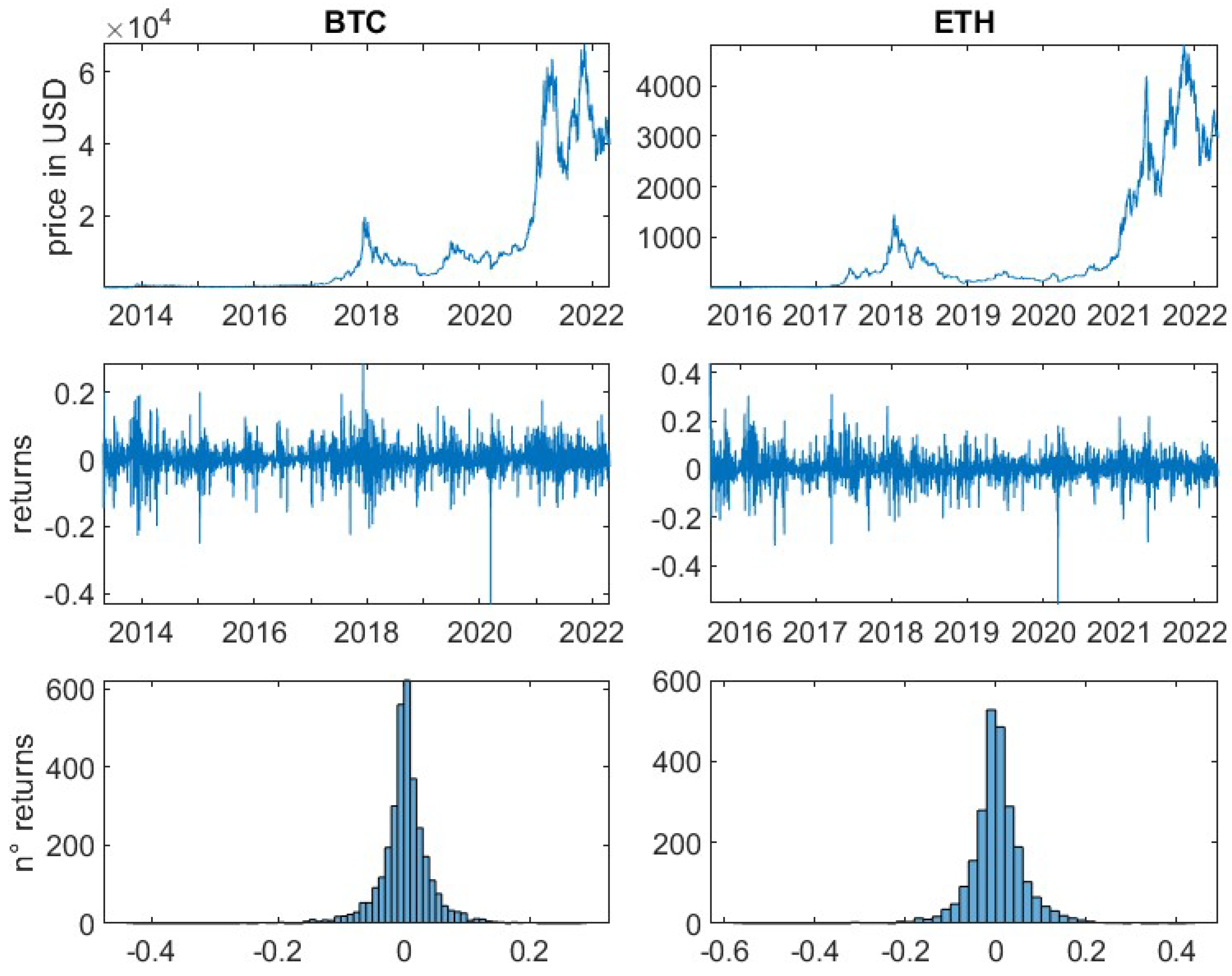
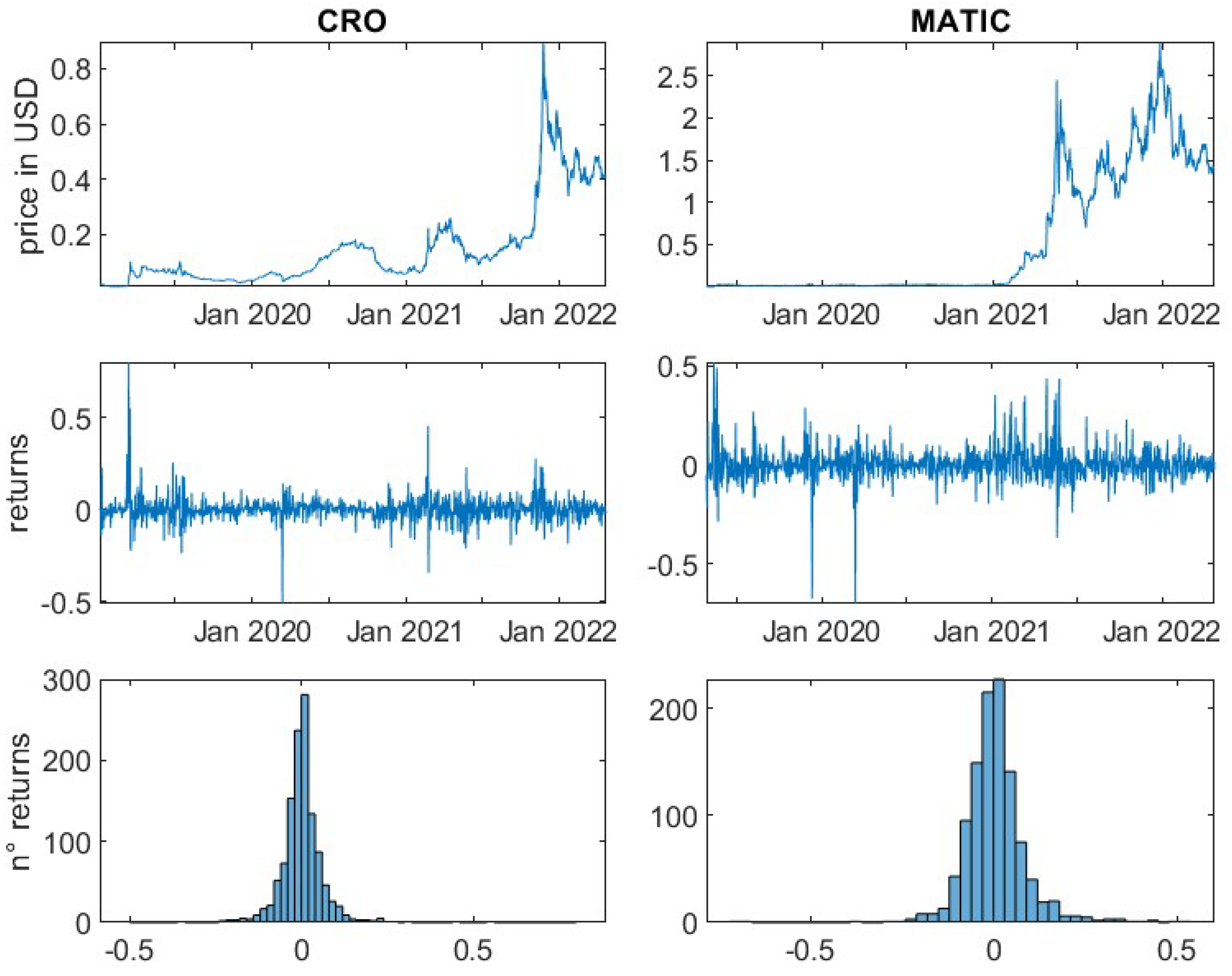
Table 3 exhibits the basic risk characteristics of the analysed portfolio. Almost all cryptocurrencies display a positive mean of the daily logarithmic returns in the range of 0.15% to 0.5%. The memecoin Shiba Inu strongly deviates from this range with a mean daily return of 1.61%. Furthermore, it is observed that cryptocurrencies with a lower number of daily returns, i.e., more recently established, possess a higher mean. This could be explained by the bull market that has been prevailing for most of its existence. A long-term investment in the portfolio would have proved to be very successful, but not without risks, as the high standard deviations indicate. For most cryptocurrencies, the daily returns deviate between 6 to 8% around the mean. Investors, therefore, must be able to compensate for the high daily fluctuations in value. They should account for this property, especially in financial transactions that require a frequent margin and collateral adjustment. The lowest standard deviation is displayed by Bitcoin, which could be explained by its relatively high market capitalisation and advanced market maturity. Hence, Bitcoin acts as a less volatile asset and a possible investment opportunity for more risk-averse cryptocurrency investors. On the contrary, Shiba Inu is the riskiest cryptocurrency in the selected portfolio with a standard deviation of 24.38%. Its investors are exposed to extreme fluctuations in daily returns.
The kurtosis of all the selected cryptocurrencies indicates that their return distributions are heavy-tailed and outlier-prone. The return distributions of Near and Solana come closest to that of a normal distribution, which is characterised by a kurtosis of 3. Furthermore, our analysis indicates that most return distributions are asymmetrically spread out towards the right. Only Bitcoin, Ethereum and Solana are characterised by a negative skewness. By computing the Value-at-Risk and the corresponding Expected-Shortfall, we can further prove the high riskiness of the selected cryptocurrencies. The VaR(99%) ranges between 12 to 20% of daily losses for most of the cryptocurrencies, whereby, Bitcoin shows the lowest VaR and Shiba Inu the highest with around 52%. Table 4 depicts the determined risk measures.
All cryptocurrencies show a positive correlation to both Bitcoin and Ethereum. Surprisingly 9 out of 12 analysed cryptocurrencies are more strongly correlated with Ethereum than Bitcoin. This is remarkable, considering the lower relative market share of Ethereum and the fact that cryptocurrencies, such as BNB, SOL, or AVAX, are considered alternative smart contract platforms that are competing with Ethereum to be the dominant ecosystem within the cryptocurrency market. A strong positive correlation seems counterintuitive and could be the subject of further research. Considering the stated high riskiness of all the selected cryptocurrencies, we apply Extreme Value Theory to investigate their extreme tail risks.
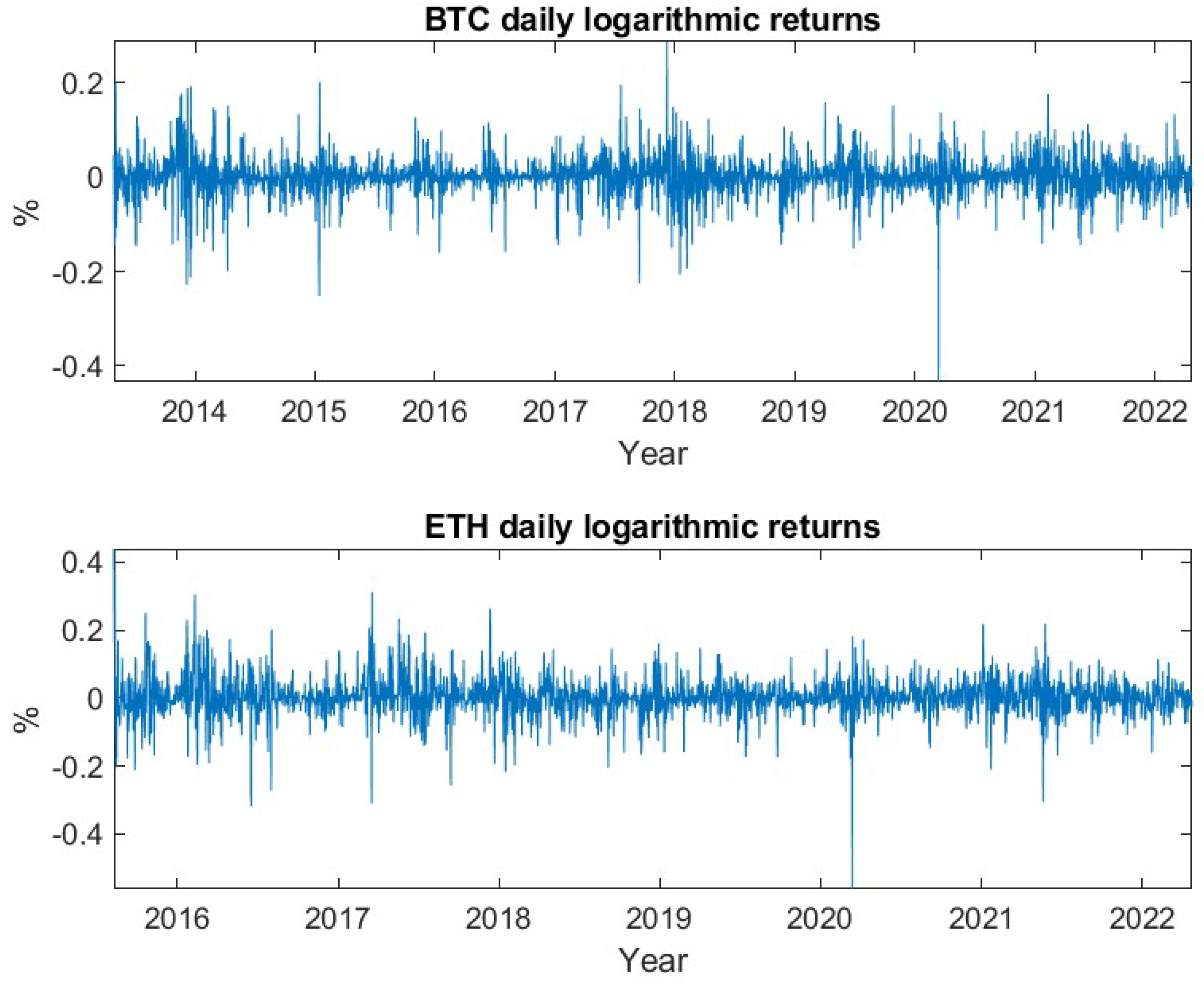
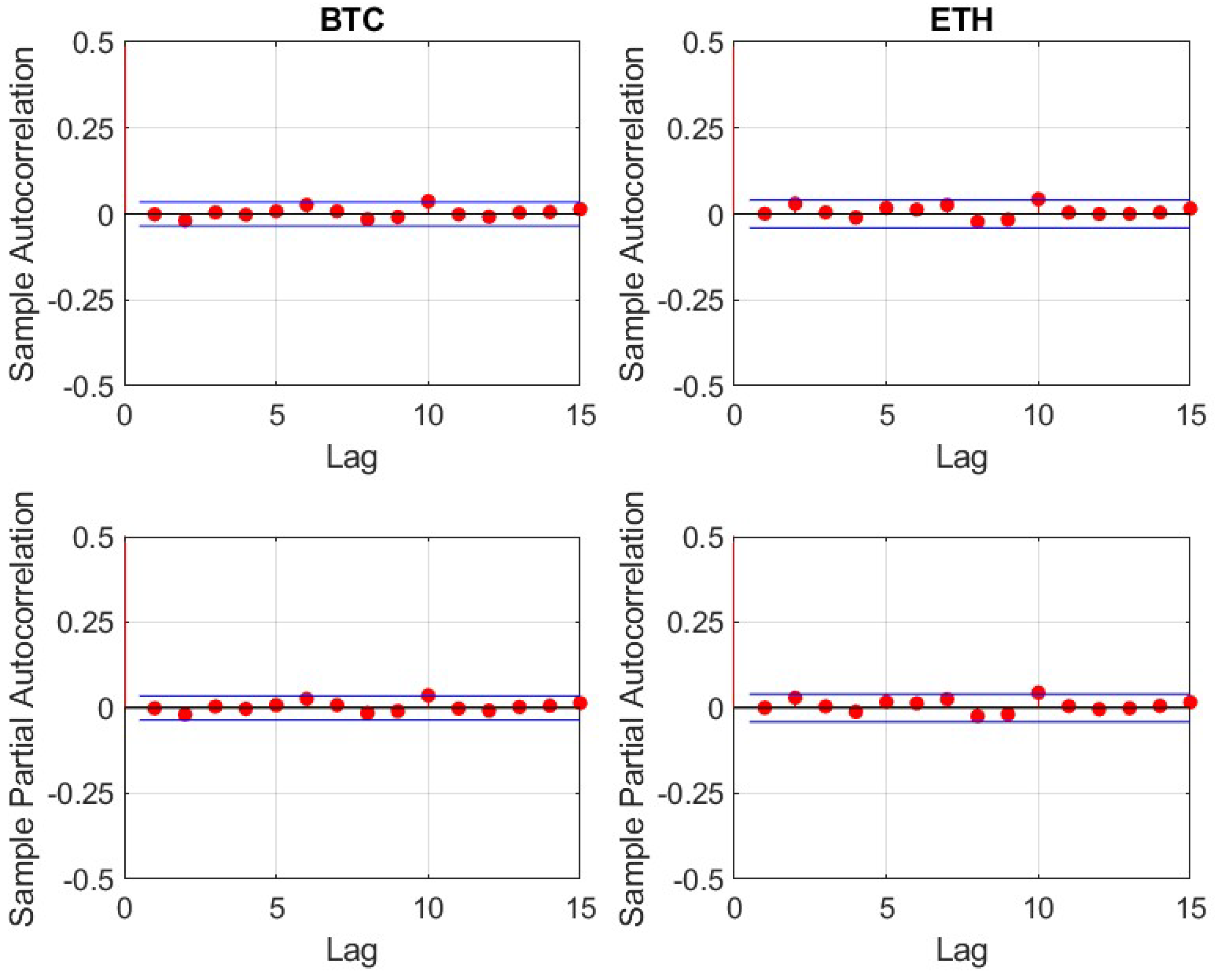
EVT is based on the simplified assumption of independent and identically distributed (iid) data, i.e., past values do not influence future outcomes and the underlying distribution is identical for all datapoints. No data clustering should be observable. Financial data often does not fulfill these characteristics. The plotted historical daily returns of BTC and ETH, as exemplary for the cryptocurrency market, lead us to doubt the iid property. Strong volatility clustering can be observed in Figure 1.
To statistically prove this presumption, a turning point test is applied. For a timeseries of data , a turning point T at time n is defined as or . For an iid series, it holds that,
Hence, we can test the iid property of the data via a hypothesis test, rejecting at the 5%-confidence level if (Brockwell and Davis 2002)
The turning point test proves that, for all the tested cryptocurrencies, the iid property is rejected at the 5% level. This is consistent with the previous presumption based on the eye criterion. It implies that the underlying assumption of EVT is not fulfilled. To overcome the resulting drawbacks, we apply the GARCH-EVT method, described by McNeil and Frey (2000).
Consider to be daily negative logarithmic returns of the analysed cryptocurrencies, denoted as
The dynamics of the conditional mean and the conditional volatility are to be modelled by an AR(1) and a GARCH(1, 1) model, whereby the process could be extended to further specialised models. AutoRegressive (AR) models predict future outcomes based on the p past observations (lags). An AR model with one lag, denoted as AR(1), uses the most recent observation to predict a future outcome. The conditional mean can therefore be represented by:
Generalized AutoRegressive Conditional Heteroskedasticity (GARCH) models are used to estimate and forecast the volatility of a time series, such as the returns of financial assets. In contrast to other models, they recognise that volatilities are not constant over time and can form clusters of periods with high or low levels (Hull 2018).
Kaya Soylu et al. (2020); Chu et al. (2017) and Katsiampa (2017) investigate the goodness-of-fit of different GARCH-models to the time series of cryptocurrency returns. Non come to the same conclusion. All favour different models for individual cryptocurrencies, during diverging observation periods. While different, specialized GARCH-variations may be best suited for the individually tested observation periods, the GARCH(1, 1) going back to Bollerslev (1986) provides reliable results throughout these different periods. Therefore, we rely on the standard GARCH model to describe the conditional volatility of the 14 time series.
The conditional variance of the GARCH(1, 1) model by Bollerslev is given by:
where and can be calculated as . is the weight assigned to the long term variance (), is the weight assigned to and is the weight assigned to , where (Bollerslev 1986). Furthermore, the model integrates mean reversion, i.e., in practice the variance tends to follow a long-term average that pulls the variance back at rate (Hull 2018).
The model is then fitted to the return data via Maximum Likelihood Estimation to obtain the estimated parameters (). If the model is well fitted, the obtained standardised residuals, calculated as:
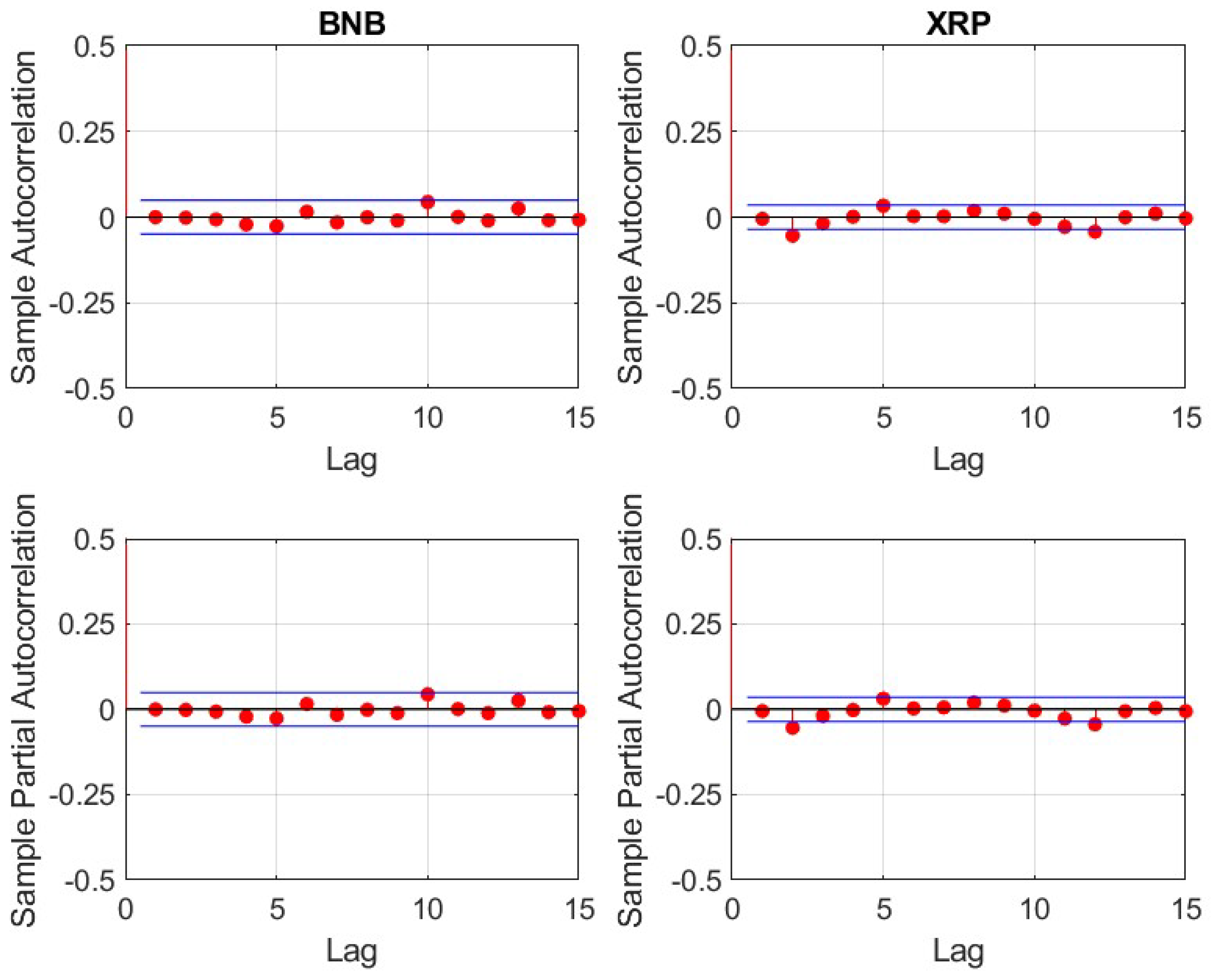
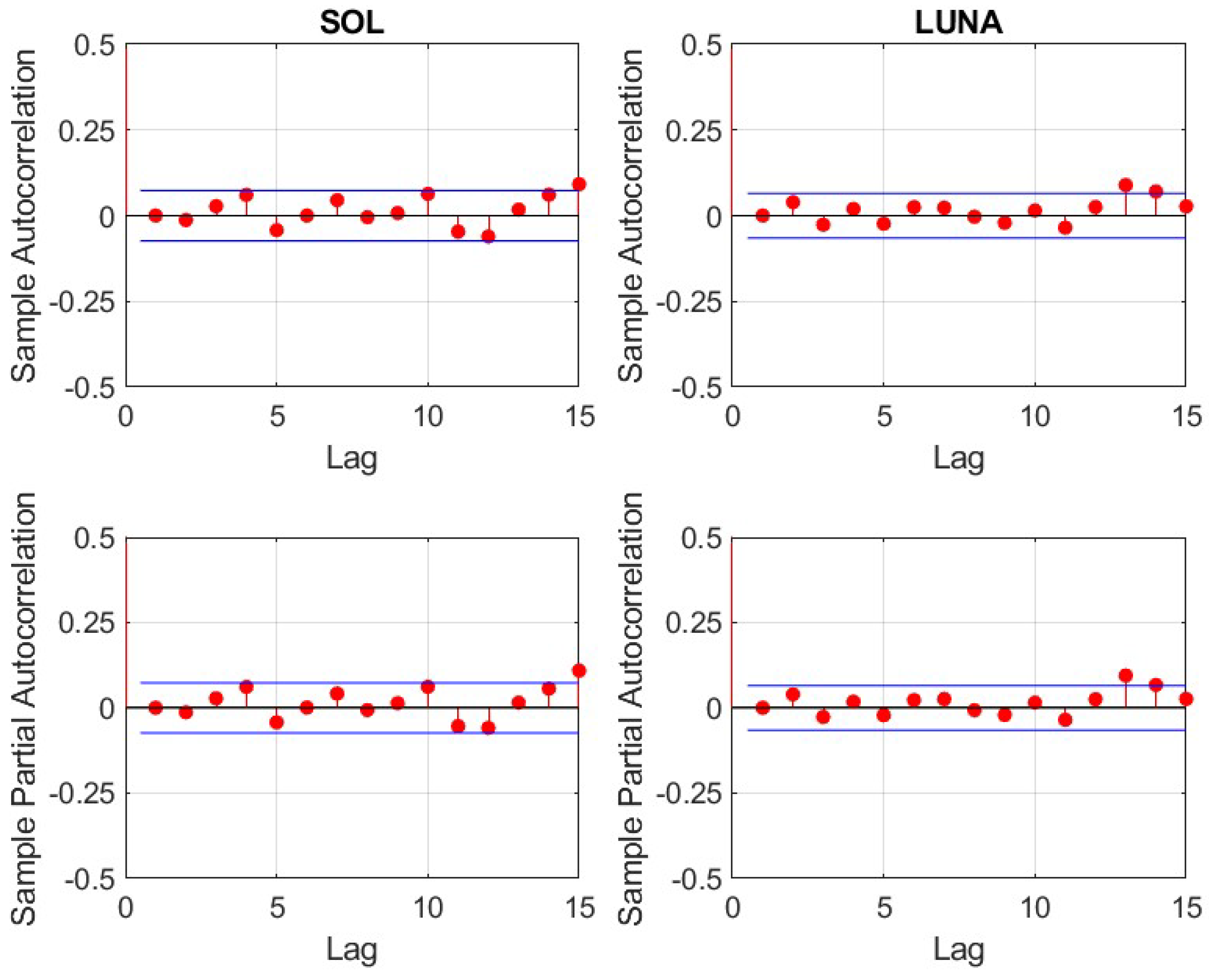
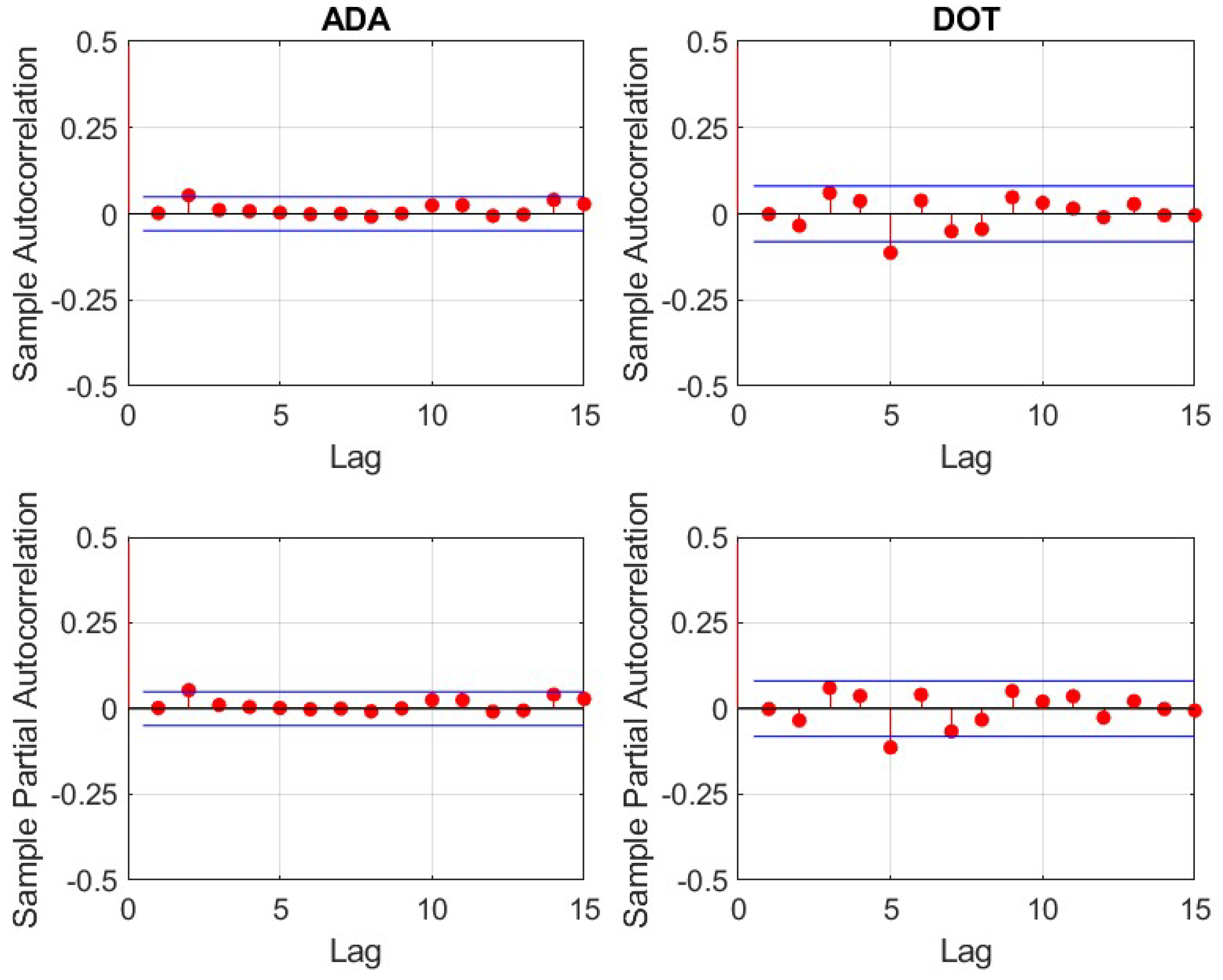
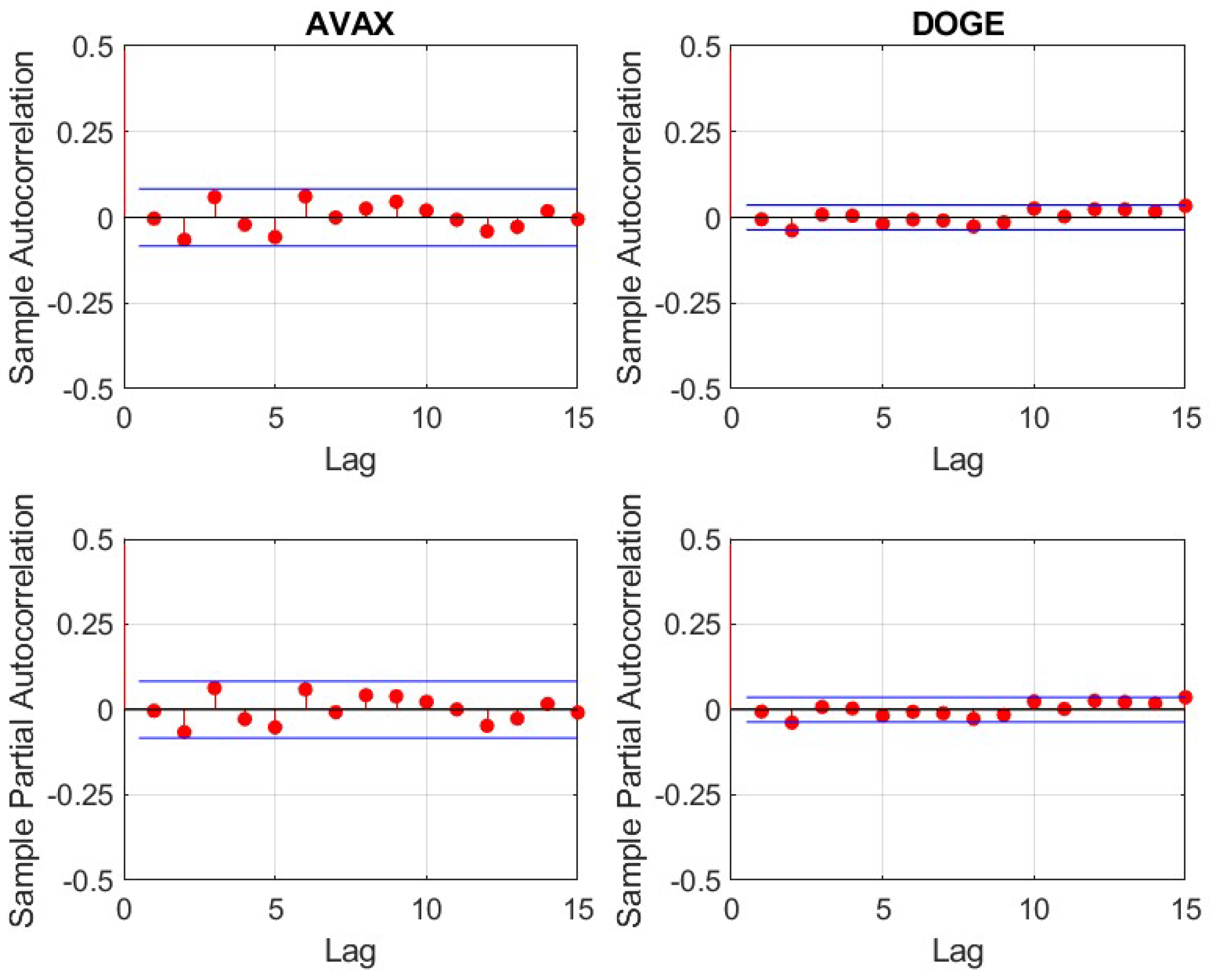
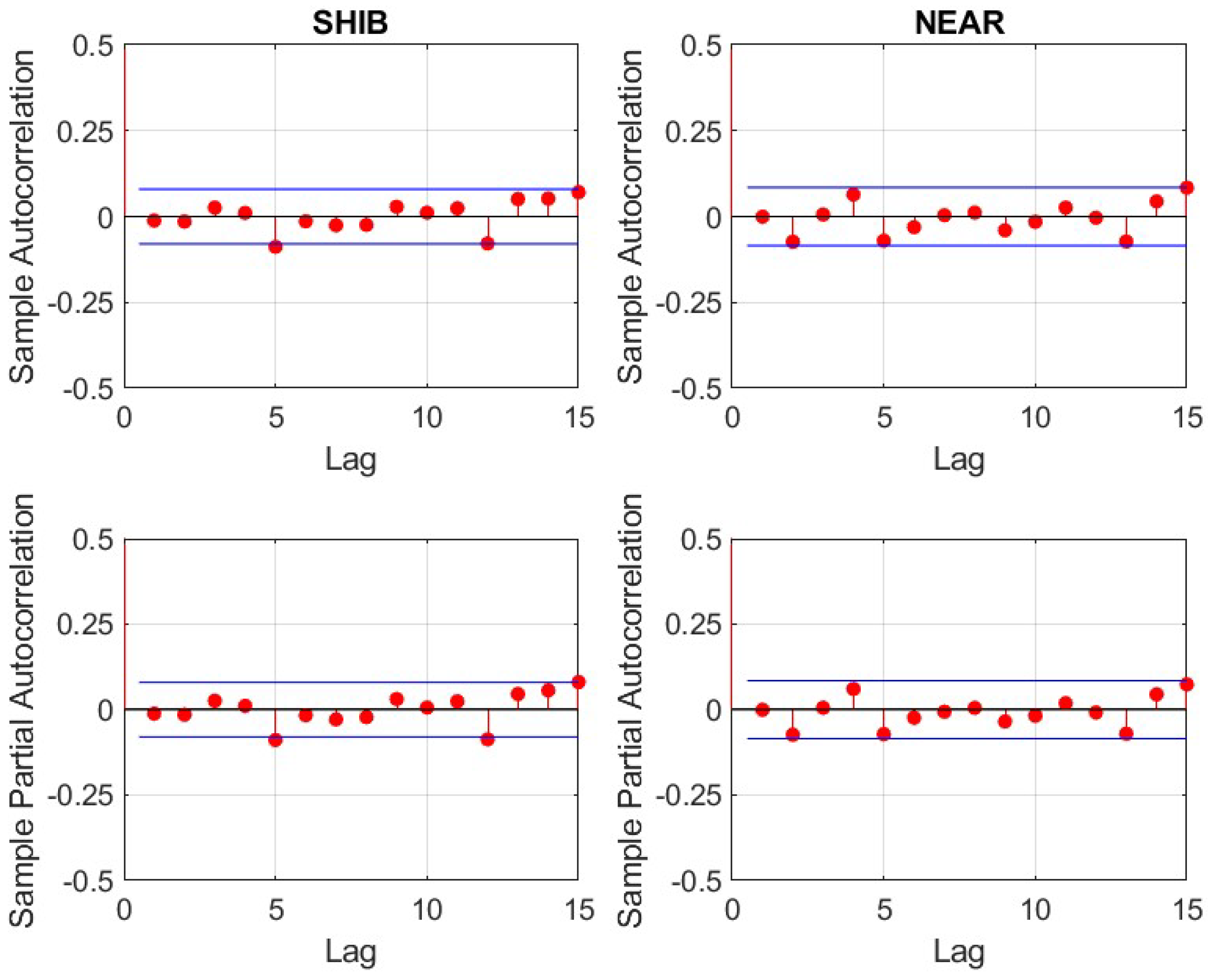
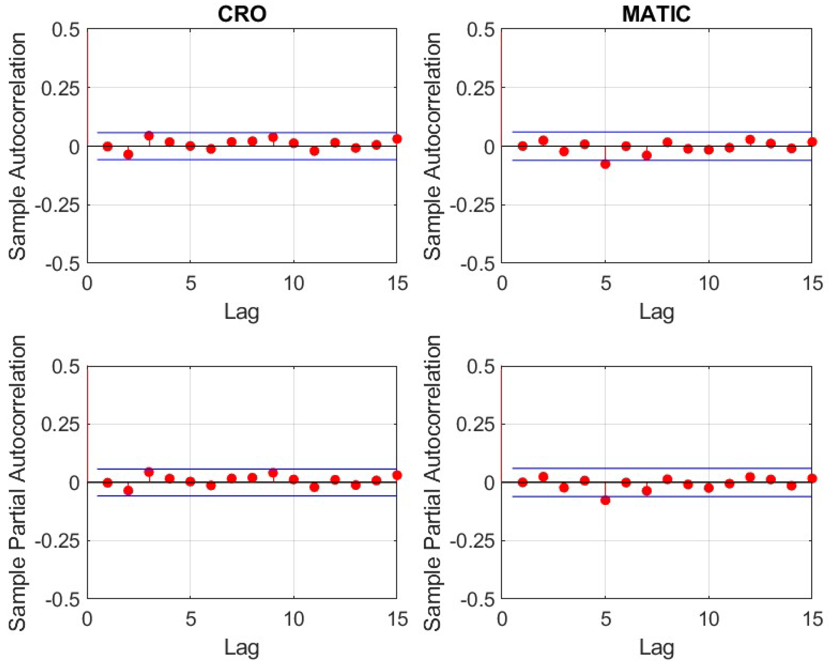
are realisation of a white noise process with the property of being at least ∼iid. To test this property the 1st to 4th order moments of the standardised residuals are computed. All 14 residual series show a mean close to 0 and variance close to 1, while a high kurtosis for all residuals series indicates that the standardised residuals show heavy tails. An Engle’s ARCH test is conducted to test for residual conditional heteroskedasticity in the standardised residuals series. The logical value 0 implies, that we cannot reject the null hypothesis of no residual heteroskedasticity in the series. Autocorrelation in the residual series is tested by applying a Ljung-Box-Q test over 15 lags. No residual autocorrelation is detected for the cryptocurrencies. The Ljung-Box-Q test for the squared residuals confirms the findings of Engle’s ARCH test. The results of this analysis can be seen in Table 5, as well as in Appendix B.
In contrast to the logarithmic return series, which have been proven not to be iid, the assumption that the standardised residuals are at least ∼iid holds. Consequently, the one-day forecast of the conditional mean and volatility can be estimated, according to Formulas (11) and (12). The EVT is then used to estimate the tail distribution of the residuals, as well as the corresponding VaR and Expected-Shortfall. Given the required forecasts, and the quantile of the residuals’ tail distribution (represented by the VaR), the VaR and the ES of the 1-step predictive distribution can be determined as:
Table 6 depicts the final risk measures resulting out of the GARCH-EVT process for all the individual cryptocurrencies.
We can observe, that all chosen cryptocurrencies are subject to high possible daily losses. These findings are in line with the results of Dutta and Bouri (2022); Gkillas et al. (2018); Omari and Ngunyi (2021), and Osterrieder and Lorenz (2017) who showed that cryptocurrencies are characterised by extreme price movements. The GARCH-EVT approach returns more conservative risk measures, compared to the previous risk assessment based on the empirical loss distributions. Solely, SHIB exhibits risk measures out-of-range, that exceed losses of 100%. This can be explained by the extreme quantiles of SHIB’s standardised residuals. Contrary to losses, they are not capped and hence can lead to unfeasible losses. It can be assumed that these values converge to losses of 100%. The estimated tail distributions allow us to determine the VaR and ES for the 99.9% quantiles. These are of high importance to calculate the respective minimum capital requirements. The daily VaRs (99.9%) fluctuate around a loss of 30%. Hence banks and other financial institutions must hold large values of capital, in order to maintain the capital adequacy ratio.
3.2. Portfolio Aggregation
So far, we have determined the properties of the logarithmic return series of 14 individual cryptocurrencies. We further examine the properties and possible diversification benefits of a portfolio of the 14 cryptocurrencies, weighted according to their respective market shares. Table 7 shows the portfolio composition. For simplicity, we fix the weights based on the current market shares and, retrospectively, calculate the returns and the properties for the last 365 trading days. The weights are held consistently over the time horizon and the transaction costs to rebalance the portfolio are neglected.
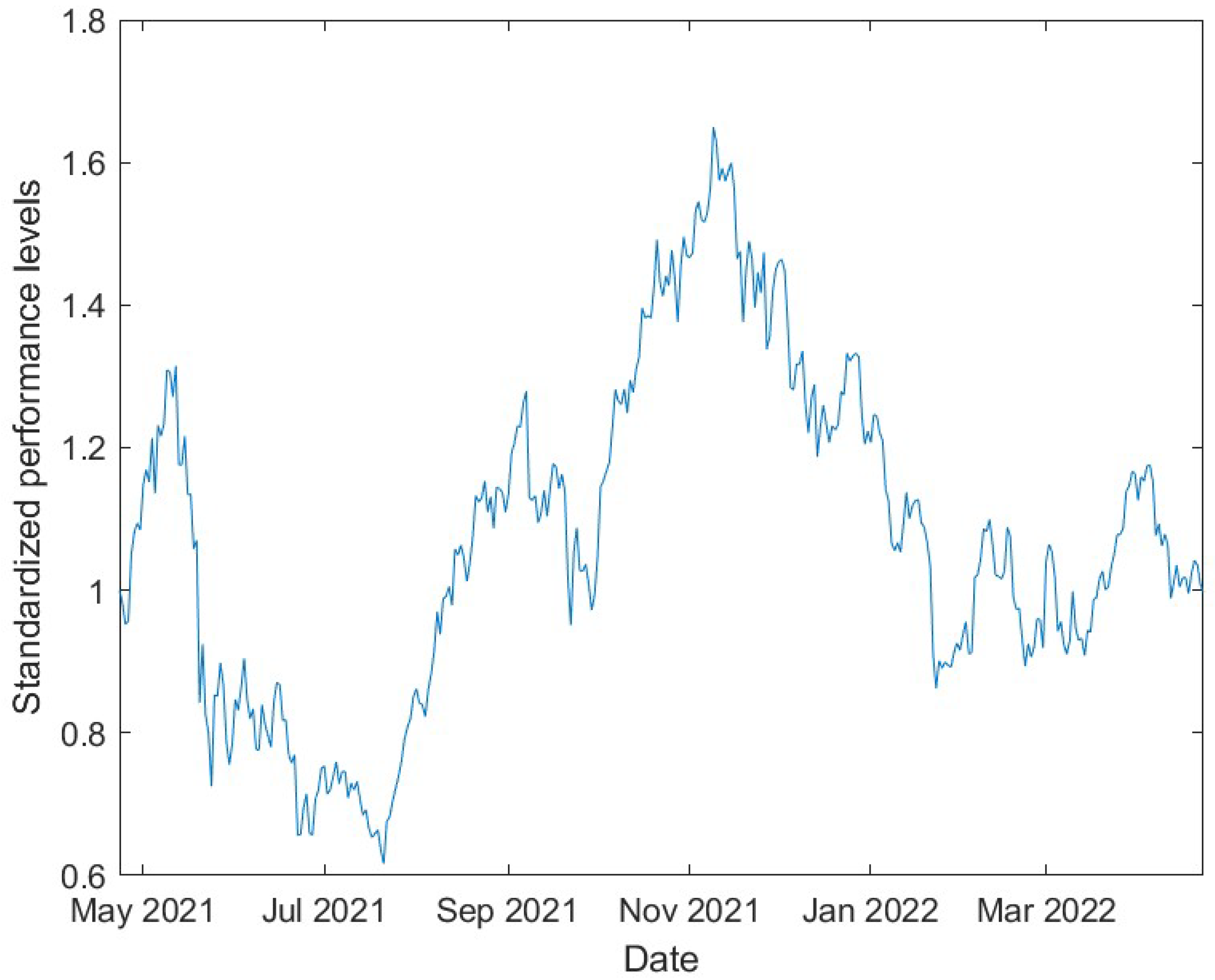
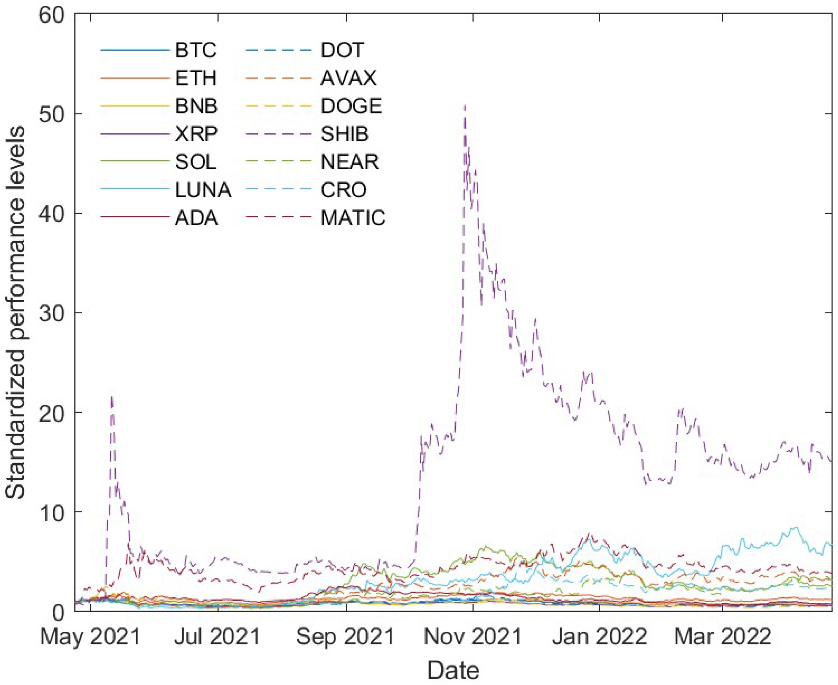
Figure 2 shows the standardised performance of the cryptocurrency portfolio, while Figure 3 depicts the performance of the individual cryptocurrencies during the investment period of 365 trading days. The returns of Shiba Inu dwarf all other performances. We can observe two extreme speculative periods of extreme price increases, followed by sharp declines in valuation. At its peak, SHIB experienced a price increase by five orders of magnitude. This observation corresponds to our previous analysis of SHIB, which detected exposures to extreme risks and fluctuations in price. Even though SHIB only represents 0.94% of the portfolio, its extraordinary performance has been a strong value driver of the selected portfolio.
Table 8 highlights the final performance of all portfolio positions over the investment period of 365 trading days. We can observe that, out of the 14 positions, eight have been profitable investments with price increases of between 1.2 to 16 times their initial valuation. Except for SOL and LUNA, those are comparatively smaller cryptocurrencies that do not contribute much weightage to our portfolio composition. No considerable fluctuation in the price of ETH can be noted, while six cryptocurrencies lost up to 50% of their initial value. BTC, as the portfolio’s largest position, lost around 25%, while DOGE realised the largest losses of almost 50%. The reason, therefore, might be the change in investors’ sentiment regarding the “meme-coin”. The speculator’s attention switched to SHIB as their new preferred “meme-coin”. This could be observed in their diverging price movements during the investment period.
Given our previous results, cryptocurrencies show heavy tails and extreme returns. We follow the approach of Luu Duc Huynh (2019) and fit a t-Student Copula to the daily logarithmic returns to estimate their joint density function. The degrees of freedom, represented by , are estimated to be 7.35. Table 9 shows the cross-correlations of the logarithmic returns of all the 14 assets in the selected portfolio.
All analysed cryptocurrencies show a remarkably high positive correlation to all other portfolio positions. All seem to behave similarly and follow the overall market sentiment. This is in accordance with the findings of Krückeberg and Scholz (2019), who came to the same conclusion by analysing cryptocurrency data up to December 2017. This property of the asset class of cryptocurrency still holds. No cryptocurrency might function as a possible hedge to the price changes of another portfolio position. Note that, including stablecoins in a cryptocurrency portfolio might change the outcome of the previous analysis. Stablecoins usually try to mimic the value of one USD. Hence, they should not function as a perfect hedge as their possible up and down movement is constrained but they should at least add bounded stability and a decrease in volatility to the portfolio. The decrease in market risks comes at the cost of third-party risks, technical risks and regulatory risks. These should not be neglected as seen in the recent events concerning the Terra Luna ecosystems and its algorithmic stablecoin Terra USD (Sandor and Genç 2022). Furthermore, we observe that most cryptocurrencies show the strongest correlation to ETH. This is also valid for cryptocurrencies, that are considered to be “Alternative Layer-Ones”, such as BNB, SOL, or ADA. This could indicate that the market does not follow the thesis of only one prevailing smart contract platform but rather believes in a multi-chain future. This is in accordance with our previous findings. It might indicate that even though Bitcoin has the largest market share, it is not the best indicator to predict future market behaviour. These results support the suggestion of Bouri et al. (2021); Shahzad et al. (2022), and Kumar et al. (2022) that monitoring procedures should comprise further leading cryptocurrencies that are net transmitters of extreme returns. Financial models, trying to predict market moves, should account for this property.
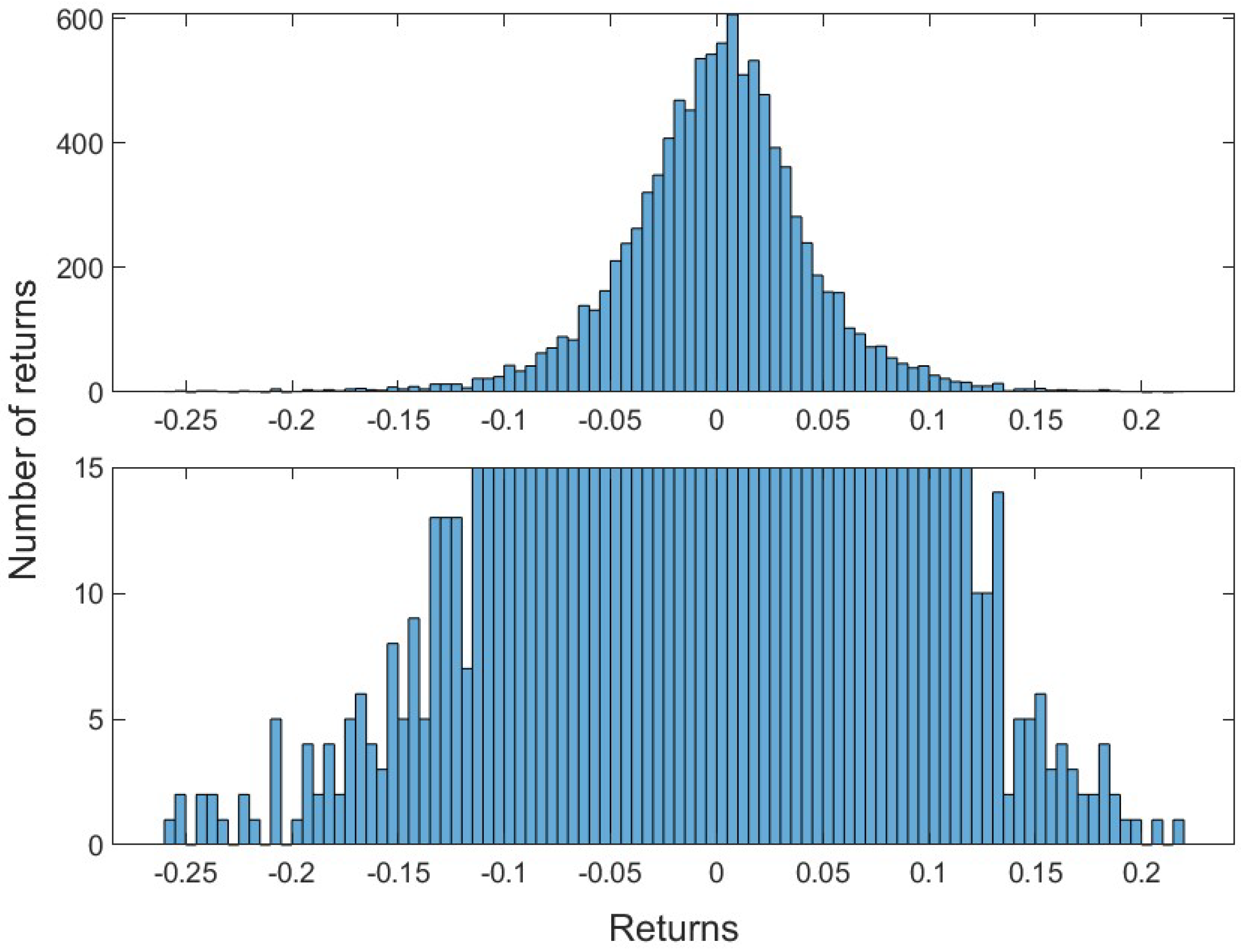
In the next step, a Monte-Carlo-Simulation is performed to simulate 10,000 densities based on the joint density function of all the portfolio positions. The densities are transformed into the corresponding daily returns of the portfolio through the inverse probability distribution. Figure 4 shows the resulting histogram of the simulated daily returns and Table 10, the corresponding maximum loss and gain. We observe that the portfolio with aggregated risks, accounting for the intra-market-correlation, is subject to heavier tails. The daily returns, denoted as a loss distribution, range between 25.64% to −21.68% and exceed the daily returns of the portfolio of individual risks, by 1.66% and 5,38%, respectively. We conclude that the portfolio, with aggregated risks, shows heavier-tailed behaviour and is more outlier-prone. This is in accordance with the findings of Luu Duc Huynh (2019) who showed that the network of contagion risks among cryptocurrencies increases the probability of joint extreme values. The diversification effect, calculated as the difference between the expected daily return of the portfolio of aggregated risks and the one with the individual risks, indicates that both portfolios yield almost similar daily returns. The expected return of the individual risks is 0.01% higher and more range bound, according to the maximum loss and gain.
Conclusively, we determine the VaR and the ES at different confidence levels for the aggregated portfolio risks and the sum of the individual risks. Consistent with our previous results, we observe higher Value-at-Risk measures for the portfolio of aggregated risks, as can be seen in Table 11. While slightly lower Expected-Shortfalls are observed for lower confidence levels and almost identical measures for the 99% level. The 99.9% level, which is important for the determination of the minimum capital requirements of banks, gives a VaR of 21.98% and an ES of 23.98%.
We can infer from the findings of our analysis that cryptocurrency investors are exposed to extreme tail behaviour, both on the positive as well on the negative side. Thus, investing in cryptocurrencies can be a profitable strategy that exposes inventors to high risks, which should be accounted for to avoid any adverse events. The risks cannot be hedged or mitigated by investing in a broader market portfolio as it does not lead to diversification benefits, but rather increases the probability of joint extreme values.
4. Discussion
This article aims to analyse the financial risk characteristics of individual cryptocurrencies and of a broad cryptocurrency market portfolio. Due to the individual observation periods, we give the reader an up-to-date risk assessment of highly relevant cryptocurrencies, representing 82.1% of the total cryptocurrency market. All cryptocurrencies show high volatility in their price movements, whereby, Bitcoin acts as the most stable cryptocurrency among the 14 tested ones. Furthermore, all return distributions are described by a high kurtosis, indicating that they exhibit a heavy-tailed behaviour that is not well described by a normal distribution. To estimate extreme tail risks, we apply the Extreme Value Theory in combination with a novel algorithm to determine the optimal threshold for the tail model. Our analysis indicates that all cryptocurrencies are subject to extreme tail risks. Hence, investors are exposed to high possible daily losses. Although the EVT offers well-founded tools to describe the extreme tails of a distribution, it cannot by any means predict the future with high accuracy. During the drafting of this article, we could witness the total collapse of the Terra Luna ecosystem, due to a decoupling of its algorithmic stablecoin Terra USD and the resulting loss of its user’s confidence. Even the Extreme Value Theory could not have predicted a loss of ∼100%.
Furthermore, we construct a broad market portfolio to test for possible diversification effects. We model the joint density function of all portfolio positions by a t-Student Copula and simulate 10,000 densities via a Monte-Carlo Simulation. Our findings indicate that all portfolio positions are highly correlated with the strongest correlation to ETH. This property has implications for the construction of models trying to predict future market behaviour. We find that, by aggregating market risks, no diversification benefit can be achieved. On the contrary, a minimal lower expected daily return can be observed. Consistent with prior research, investing in a broad market portfolio leads to higher joint extreme returns, both positive as well as negative. By investing in individual cryptocurrencies or in a portfolio, investors are exposed to possible high daily losses. This must be incorporated into an investor’s risk management to avoid adverse events, such as margin calls due to the failure to provide sufficient funds to cover against tail risks. Additionally, our results have important implications for banks or investment vehicles. The determined risk measures indicate that high minimum capital requirements are to be expected by regulators, in order to compensate for the additional riskiness. Investors must evaluate the impact of binding additional equity on their profitability. We join Bouri et al. (2021) and Kumar et al. (2022), in suggesting a broader approach to market regulation and policy. Given the implications extreme market conditions have on the cryptocurrency market and the importance smaller cryptocurrencies take on, current monitoring processes should be extended to larger parts of the market.
We identified multiple topics for future research that could widen the understanding of the cryptocurrency market. First, the market behaviour, hedging properties as well as possible benefits of a portfolio composition with stablecoins remain to be investigated. Second, the identification of the best-suited Copula, to model the joint density function of a cryptocurrency portfolio. Furthermore, the cryptocurrency market can no longer be described by its two largest cryptocurrencies. Hence, an analysis of the properties and intra-market correlations between different sectors within the market, as well as within different ecosystems on smart contract platforms would be of interest to market participants. The implications of the above-mentioned research questions for legislators and regulators remain to be investigated.
Finally, we want to remark that despite the identified high riskiness that an investment in this market bears, investors should not neglect this emergent market and its opportunities. Labelling cryptocurrencies as purely speculative and risky would be pre-emptive. Risk-averse investors should, rather, familiarise themselves with the cryptocurrency market, its underlying technologies and value propositions. Once the conditions are suitable to their own or their client’s expectations a market entry can be re-evaluated.
Author Contributions
Conceptualization, P.B. and D.E.; methodology, P.B.; software, P.B.; validation, P.B.; formal analysis, P.B.; investigation, P.B.; resources, D.E.; data curation, P.B.; writing—original draft preparation, P.B.; writing—review and editing, D.E.; visualization, P.B.; supervision, D.E.; project administration, D.E.; funding acquisition, D.E. All authors have read and agreed to the published version of the manuscript.
Funding
The article processing charge was funded by the Ministerium für Wissenschaft, Forschung und Kunst Baden-Württemberg and Nürtingen-Geislingen University in the funding programme Open Access Publishing.
Institutional Review Board Statement
Not applicable.
Informed Consent Statement
Not applicable.
Data Availability Statement
The data was obtained from https://www.coingecko.com/, as described in Section 2.
Acknowledgments
We thank Christoph J. Börner (Heinrich Heine University Düsseldorf) for providing the algorithm Find The Tail (FTT) and for helpful advices.
Conflicts of Interest
The authors declare no conflict of interest.
Abbreviations
The following abbreviations are used in this manuscript:
| AD | Anderson-Darling test |
| ADA | Cardano |
| AR | AutoRegressive |
| ARCH | AutoRegressive Conditional Heteroskedasticity |
| AVAX | Avalanche |
| BTC | Bitcoin |
| CRO | Cronos |
| CvM | Cramér-von Mises test |
| DOGE | Dogecoin |
| DOT | Polkadot |
| ES | Expected-Shortfall |
| ETH | Ethereum |
| EVT | Extreme-Value-Theory |
| GARCH | Generalized AutoRegressive Conditional Heteroskedasticity |
| GPD | Generalized Pareto Distribution |
| iid | independent and identically distributed |
| LUNA | Terra |
| MATIC | Polygon |
| NEAR | Near Protocol |
| POTM | Peaks-Over-Threshold-Method |
| SHIB | Shiba Inu |
| SOL | Solana |
| USD | United States Dollar |
| VaR | Value-at-Risk |
Appendix A
Figure A1.
BTC and ETH daily logarithmic returns.

Figure A2.
BNB and XRP daily logarithmic returns.

Figure A3.
SOL and LUNA daily logarithmic returns.

Figure A4.
ADA and DOT daily logarithmic returns.

Figure A5.
AVAX and DOGE daily logarithmic returns.

Figure A6.
SHIB and NEAR daily logarithmic returns.

Figure A7.
CRO and MATIC daily logarithmic returns.

Appendix B
Figure A8.
BTC’s and ETH’s residuals’ autocorrelation.

Figure A9.
BNB’s and XRP’s residuals’ autocorrelation.

Figure A10.
SOL’s and LUNA’s residuals’ autocorrelation.

Figure A11.
ADA’s and DOT’s residuals’ autocorrelation.

Figure A12.
AVAX’s and DOGE’s residuals’ autocorrelation.

Figure A13.
SHIB’s and NEAR’s residuals’ autocorrelation.

Figure A14.
CRO’s and MATIC’s residuals’ autocorrelation.

References
- Acereda, Beatriz, Angel Leon, and Juan Mora. 2020. Estimating the expected shortfall of cryptocurrencies: An evaluation based on backtesting. Finance Research Letters 33: 101181. [Google Scholar] [CrossRef]
- Ahmad, Muhammad Idrees, Crawford D. Sinclair, and Barrie D. Spurr. 1988. Assessment of flood frequency models using empirical distribution function statistics. Water Resources Research 24: 1323–28. [Google Scholar] [CrossRef]
- Arli, Denni, Patrick van Esch, Marat Bakpayev, and Andrea Laurence. 2020. Do consumers really trust cryptocurrencies? Marketing Intelligence & Planning 39: 74–90. [Google Scholar] [CrossRef]
- BCBS. 2005. An Explanatory Note on the Basel II IRB Risk Weight Functions. Basel: Bank for International Settlements. [Google Scholar]
- BCBS. 2009. Observed Range of Practice in Key Elements of Advanced Measurement Approaches (AMA). Basel: Bank for International Settlements. [Google Scholar]
- Binance. 2022. What Is BNB? Available online: https://academy.binance.com/en/articles/what-is-bnb (accessed on 12 May 2022).
- BitGo. 2018. WBTC Brings Bitcoin to Ethereum. Available online: https://www.coingecko.com/en/global_charts (accessed on 12 May 2022).
- Bitstamp. 2022. Bitstamp Crypto Pulse. Available online: https://www.bitstamp.net/crypto-pulse/ (accessed on 12 May 2022).
- Bollerslev, Tim. 1986. Generalized autoregressive conditional heteroskedasticity. Journal of Econometrics 31: 307–27. [Google Scholar] [CrossRef] [Green Version]
- Borri, Nicola. 2019. Conditional tail-risk in cryptocurrency markets. Journal of Empirical Finance 50: 1–19. [Google Scholar] [CrossRef]
- Bouri, Elie, Tareq Saeed, Xuan Vinh Vo, and David Roubaud. 2021. Quantile connectedness in the cryptocurrency market. Journal of International Financial Markets, Institutions and Money 71: 101302. [Google Scholar] [CrossRef]
- Brockwell, Peter J., and Richard A. Davis. 2002. Introduction to Time Series and Forecasting, 2nd ed. Springer Texts in Statistics. New York: Springer. [Google Scholar]
- Bruhn, Pascal. 2022. FindTheTail—Extreme Value Theory. Available online: https://github.com/PascalBruhn/FindTheTail/releases/tag/v1.1.1 (accessed on 27 June 2022).
- Börner, Christoph J., Ingo Hoffmann, Jonas Krettek, Lars Kuerzinger, and Tim Schmitz. 2021. On the Return Distributions of a Basket of Cryptocurrencies and Subsequent Implications. SSRN Electronic Journal. Available online: https://papers.ssrn.com/sol3/papers.cfm?abstract_id=3851563 (accessed on 12 May 2022).
- Cheikh, Nidhaleddine Ben, Younes Ben Zaied, and Julien Chevallier. 2020. Asymmetric volatility in cryptocurrency markets: New evidence from smooth transition GARCH models. Finance Research Letters 35: 101293. [Google Scholar] [CrossRef]
- Chu, Jeffrey, Stephen Chan, Saralees Nadarajah, and Joerg Osterrieder. 2017. GARCH Modelling of Cryptocurrencies. Journal of Risk and Financial Management 10: 17. [Google Scholar] [CrossRef]
- CoinGecko. n.d.a All Cryptocurrencies. Available online: https://www.coingecko.com/en (accessed on 12 May 2022).
- CoinGecko. n.d.b Cryptocurrency Global Charts. Available online: https://www.coingecko.com/en/global_charts (accessed on 12 May 2022).
- Corbet, Shaen, Brian M. Lucey, Andrew Urquhart, and Larisa Yarovaya. 2018. Cryptocurrencies as a Financial Asset: A Systematic Analysis. SSRN Electronic Journal. Available online: https://papers.ssrn.com/sol3/papers.cfm?abstract_id=3143122 (accessed on 12 May 2022).
- Dutta, Anupam, and Elie Bouri. 2022. Outliers and time-varying jumps in the cryptocurrency markets. Journal of Risk and Financial Management 15: 128. [Google Scholar] [CrossRef]
- Embrechts, Paul, Claudia Klüppelberg, and Thomas Mikosch. 1997. Modelling Extremal Events for Insurance and Finance. New York: Springer. [Google Scholar]
- Embrechts, Paul, Filip Lindskog, and Alexander Mcneil. 2003. Modelling Dependence with Copulas and Applications to Risk Management. In Handbook of Heavy Tailed Distributions in Finance. Amsterdam: Elsevier, pp. 329–34. [Google Scholar] [CrossRef]
- Fakhfekh, Mohamed, and Ahmed Jeribi. 2020. Volatility dynamics of crypto-currencies’ returns: Evidence from asymmetric and long memory GARCH models. Research in International Business and Finance 51: 101075. [Google Scholar] [CrossRef]
- Fang, Fan, Carmine Ventre, Michail Basios, Leslie Kanthan, David Martinez-Rego, Fan Wu, and Lingbo Li. 2022. Cryptocurrency trading: A comprehensive survey. Financial Innovation 8: 13. [Google Scholar] [CrossRef]
- Fatás, Antonio. 2019. The Economics of Fintech and Digital Currencies. OCLC: 1112357480. London: CEPR Press. [Google Scholar]
- Gkillas, Konstantinos, Stelios Bekiros, and Costas Siriopoulos. 2018. Extreme Correlation in Cryptocurrency Markets. SSRN Electronic Journal. Available online: https://papers.ssrn.com/sol3/papers.cfm?abstract_id=3180934 (accessed on 27 February 2022).
- Gkillas, Konstantinos, and Paraskevi Katsiampa. 2018. An application of extreme value theory to cryptocurrencies. Economics Letters 164: 109–11. [Google Scholar] [CrossRef] [Green Version]
- Grauer, Kim, Will Kueshner, and Henry Updegrave. 2022. 2021 NFT Market Report. New York: Chainalysis. [Google Scholar]
- Haq, Inzamam Ul, Apichit Maneengam, Supat Chupradit, Wanich Suksatan, and Chunhui Huo. 2021. Economic Policy Uncertainty and Cryptocurrency Market as a Risk Management Avenue: A Systematic Review. Risks 9: 163. [Google Scholar] [CrossRef]
- Hoffmann, Ingo. 2015. Extremwertstatistik im Portfoliomanagement. Available online: https://www.birkenland.de/extremwertstatistik-im-portfoliomanagement (accessed on 27 February 2022).
- Hoffmann, Ingo, and Christoph J. Börner. 2020a. Body and tail: An automated tail-detecting procedure. Journal of Risk 23: 43–69. [Google Scholar] [CrossRef]
- Hoffmann, Ingo, and Christoph J. Börner. 2020b. Tail models and the statistical limit of accuracy in risk assessment. The Journal of Risk Finance 21: 201–16. [Google Scholar] [CrossRef]
- Hoffmann, Ingo, and Christoph J. Börner. 2021. The risk function of the goodness-of-fit tests for tail models. Statistical Papers 62: 1853–69. [Google Scholar] [CrossRef] [Green Version]
- Hon, Henry, Kevin Wang, Michael Bolger, William Wu, and Joy Zhou. 2022. Crypto Market Sizing Global Crypto Owners Reaching 300M. Crypto.com, January 20. [Google Scholar]
- Huang, Xinyu, Weihao Han, David Newton, Emmanouil Platanakis, Dimitrios Stafylas, and Charles M. Sutcliffe. 2021. The Diversification Benefits of Cryptocurrency Asset Categories and Estimation Risk: Pre and Post COVID-19. SSRN Electronic Journal. Available online: https://papers.ssrn.com/sol3/papers.cfm?abstract_id=3894874 (accessed on 27 February 2022).
- Hull, John. 2018. Options, Futures, and Other Derivatives, 10th ed. Chennai: Pearson. [Google Scholar]
- Jalal, Raja Nabeel-Ud-Din, Ilan Alon, and Andrea Paltrinieri. 2021. A bibliometric review of cryptocurrencies as a financial asset. Technology Analysis & Strategic Management. [Google Scholar] [CrossRef]
- Jeribi, Ahmed, and Mohamed Fakhfekh. 2021. Portfolio management and dependence structure between cryptocurrencies and traditional assets: evidence from FIEGARCH-EVT-Copula. Journal of Asset Management 22: 224–39. [Google Scholar] [CrossRef]
- Katsiampa, Paraskevi. 2017. Volatility estimation for Bitcoin: A comparison of GARCH models. Economics Letters 158: 3–6. [Google Scholar] [CrossRef] [Green Version]
- Kaya Soylu, Pınar, Mustafa Okur, Özgür Çatıkkaş, and Z. Ayca Altintig. 2020. Long Memory in the Volatility of Selected Cryptocurrencies: Bitcoin, Ethereum and Ripple. Journal of Risk and Financial Management 13: 107. [Google Scholar] [CrossRef]
- Krückeberg, Sinan, and Peter Scholz. 2019. Cryptocurrencies as an Asset Class. In Cryptofinance and Mechanisms of Exchange. Edited by Stéphane Goutte, Khaled Guesmi and Samir Saadi. Series Title: Contributions to Management Science; Cham: Springer International Publishing, pp. 1–28. [Google Scholar] [CrossRef]
- Kumar, Ashish, Najaf Iqbal, Subrata Kumar Mitra, Ladislav Kristoufek, and Elie Bouri. 2022. Connectedness among major cryptocurrencies in standard times and during the COVID-19 outbreak. Journal of International Financial Markets, Institutions and Money 77: 101523. [Google Scholar] [CrossRef]
- Luu Duc Huynh, Toan. 2019. Spillover Risks on Cryptocurrency Markets: A Look from VAR-SVAR Granger Causality and Student’s-t Copulas. Journal of Risk and Financial Management 12: 52. [Google Scholar] [CrossRef] [Green Version]
- Ly, Sel, Kim-Hung Pho, Sal Ly, and Wing-Keung Wong. 2019. Determining Distribution for the Quotients of Dependent and Independent Random Variables by Using Copulas. Journal of Risk and Financial Management 12: 42. [Google Scholar] [CrossRef] [Green Version]
- Malladi, Rama K., and Prakash L. Dheeriya. 2021. Time series analysis of Cryptocurrency returns and volatilities. Journal of Economics and Finance 45: 75–94. [Google Scholar] [CrossRef]
- McNeil, Alexander J., and Rüdiger Frey. 2000. Estimation of tail-related risk measures for heteroscedastic financial time series: An extreme value approach. Journal of Empirical Finance 7: 271–300. [Google Scholar] [CrossRef]
- Nikolova, Venelina, Juan E. Trinidad Segovia, Manuel Fernández-Martínez, and Miguel Angel Sánchez-Granero. 2020. A Novel Methodology to Calculate the Probability of Volatility Clusters in Financial Series: An Application to Cryptocurrency Markets. Mathematics 8: 1216. [Google Scholar] [CrossRef]
- Omari, Cyprian, and Anthony Ngunyi. 2021. The Predictive Performance of Extreme Value Analysis Based-Models in Forecasting the Volatility of Cryptocurrencies. Journal of Mathematical Finance 11: 438–65. [Google Scholar] [CrossRef]
- Osterrieder, Joerg, and Julian Lorenz. 2017. A statistical risk assessment of Bitcoin and its extreme tail behaviour. Annals of Financial Economics 12: 1750003. [Google Scholar] [CrossRef]
- Sandor, Krisztian, and Ekin Genç. 2022. The Fall of Terra: A Timeline of the Meteoric Rise and Crash of UST and LUNA. Available online: https://www.coindesk.com/learn/the-fall-of-terra-a-timeline-of-the-meteoric-rise-and-crash-of-ust-and-luna/ (accessed on 12 May 2022).
- Schmitz, Tim, and Ingo Hoffmann. 2020. Re-evaluating cryptocurrencies’ contribution to portfolio diversification—A portfolio analysis with special focus on German investors. arXiv arXiv:2006.06237. [Google Scholar] [CrossRef]
- Schuhmacher, Frank, and Benjamin R. Auer. 2015. Extremwerttheorie und Value-at-Risk. WiSt—Wirtschaftswissenschaftliches Studium 44: 259–67. [Google Scholar] [CrossRef]
- Shahzad, Syed Jawad Hussain, Elie Bouri, Tanveer Ahmad, and Muhammad Abubakr Naeem. 2022. Extreme tail network analysis of cryptocurrencies and trading strategies. Finance Research Letters 44: 102106. [Google Scholar] [CrossRef]
- Sklar, Abe. 1959. Fonctions de Répartition à n Dimensions et Leurs Marges. Publications de l’Institut Statistique de l’Université de Paris 8: 229–31. [Google Scholar]
- Trimborn, Simon, Mingyang Li, and Wolfgang Karl Härdle. 2020. Investing with Cryptocurrencies—A Liquidity Constrained Investment Approach. Journal of Financial Econometrics 18: 280–306. [Google Scholar] [CrossRef] [Green Version]
- Wang, Kevin. 2021. Measuring Global Crypto Users: A Study to Measure Market Size Using On-Chain Metrics. Crypto.com. July. Available online: https://crypto.com/images/202107_DataReport_OnChain_Market_Sizing.pdf (accessed on 12 May 2022).
- Zeder, Markus. 2007. Extreme Value Theory im Risikomanagement, 1st ed. Zürich: Versus-Verl. [Google Scholar]
Figure 1.
BTC and ETH daily logarithmic returns.

Figure 2.
Standardised performance of the cryptocurrency portfolio.

Figure 3.
Standardised performance of the individual portfolio positions.

Figure 4.
Histogram of the simulated daily portfolio returns.


Table 1.
The 56 largest cryptocurrencies, by market capitalisation (CoinGecko n.d.a).
Table 1.
The 56 largest cryptocurrencies, by market capitalisation (CoinGecko n.d.a).
| # | Cryptocurrency 1 | Market Cap | % | Cum. | # | Cryptocurrency | Market Cap | % | Cum. |
|---|---|---|---|---|---|---|---|---|---|
| 1 | Bitcoin | $755,480,804,367 | 38.58% | 38.58% | 29 | Leo token | $5,485,069,820 | 0.28% | 85.25% |
| 2 | Ethereum | $359,109,476,826 | 18.34% | 56.93% | 30 | OKB | $5,084,448,767 | 0.26% | 85.51% |
| 3 | Tether | $83,111,769,128 | 4.24% | 61.17% | 31 | Stellar | $4,873,774,723 | 0.25% | 85.76% |
| 4 | BNB | $68,875,516,103 | 3.52% | 64.69% | 32 | Algorand | $4,886,101,910 | 0.25% | 86.01% |
| 5 | USDC | $49,948,714,500 | 2.55% | 67.24% | 33 | Monero | $4,834,611,379 | 0.25% | 86.25% |
| 6 | XRP | $35,159,949,030 | 1.80% | 69.03% | 34 | Ethereum Classic | $4,766,428,183 | 0.24% | 86.50% |
| 7 | Solana | $33,927,280,085 | 1.73% | 70.77% | 35 | Apecoin | $4,202,111,982 | 0.21% | 86.71% |
| 8 | Terra | $33,224,186,611 | 1.70% | 72.46% | 36 | Uniswap | $4,127,807,840 | 0.21% | 86.92% |
| 9 | Cardano | $29,112,897,107 | 1.49% | 73.95% | 37 | Vechain | $3,898,381,771 | 0.20% | 87.12% |
| 10 | Polkadot | $20,319,429,463 | 1.04% | 74.99% | 38 | Hedera | $3,869,784,576 | 0.20% | 87.32% |
| 11 | Avalanche | $20,103,925,464 | 1.03% | 76.02% | 39 | Filecoin | $3,726,574,277 | 0.19% | 87.51% |
| 12 | Dogecoin | $18,116,746,884 | 0.93% | 76.94% | 40 | Internet computer | $3,740,108,910 | 0.19% | 87.70% |
| 13 | Terra USD | $18,044,096,882 | 0.92% | 77.86% | 41 | Axie infinity | $3,580,419,875 | 0.18% | 87.88% |
| 14 | Binance USD | $17,624,979,619 | 0.90% | 78.76% | 42 | Elrond | $3,461,541,736 | 0.18% | 88.06% |
| 15 | Shiba Inu | $13,359,113,750 | 0.68% | 79.44% | 43 | The Sandbox | $3,198,081,787 | 0.16% | 88.22% |
| 16 | Wrapped Bitcoin | $11,134,297,499 | 0.57% | 80.01% | 44 | Theta Network | $3,196,582,322 | 0.16% | 88.39% |
| 17 | Lido Staked Ether | $10,482,439,780 | 0.54% | 80.55% | 45 | Decentraland | $3,103,078,471 | 0.16% | 88.54% |
| 18 | Near Protocol | $10,503,911,531 | 0.54% | 81.09% | 46 | Ceth | $2,903,534,400 | 0.15% | 88.69% |
| 19 | Cronos | $10,153,576,036 | 0.52% | 81.60% | 47 | Fantom | $2,845,279,842 | 0.15% | 88.84% |
| 20 | Polygon | $9,776,566,142 | 0.50% | 82.10% | 48 | MIM | $2,821,848,902 | 0.14% | 88.98% |
| 21 | Dai | $8,732,068,714 | 0.45% | 82.55% | 49 | Tezos | $2,729,498,108 | 0.14% | 89.12% |
| 22 | Bonded Luna | $7,869,175,223 | 0.40% | 82.95% | 50 | Frax | $2,697,179,805 | 0.14% | 89.26% |
| 23 | Litecoin | $7,521,474,784 | 0.38% | 83.34% | 51 | Pancakeswap | $2,697,119,158 | 0.14% | 89.40% |
| 24 | Tron | $6,921,097,001 | 0.35% | 83.69% | 52 | Klaytn | $2,627,831,057 | 0.13% | 89.53% |
| 25 | Cosmos Hub | $6,809,666,781 | 0.35% | 84.04% | 53 | Thorchain | $2,614,991,172 | 0.13% | 89.67% |
| 26 | Chainlink | $6,454,346,289 | 0.33% | 84.37% | 54 | EOS | $2,489,027,021 | 0.13% | 89.79% |
| 27 | Bitcoin Cash | $6,102,052,425 | 0.31% | 84.68% | 55 | The Graph | $2,455,901,278 | 0.13% | 89.92% |
| 28 | FTX token | $5,676,427,867 | 0.29% | 84.97% | 56 | Aave | $2,407,212,862 | 0.12% | 90.04% |
1 The names of the cryptocurrencies are depicted as given by CoinGecko and do not necessarily represent their true names. See Ethereum (Ether) as an example.
Table 2.
Selected portfolio of cryptocurrencies.
| # | Cryptocurrency 1 | Earliest Date | Latest Date | Days | Market Cap | % | Cum. |
|---|---|---|---|---|---|---|---|
| 1 | Bitcoin (BTC) | 28/04/2013 | 23/04/2022 | 3283 | $755,480,804,367 | 38.58% | 38.58% |
| 2 | Ethereum (ETH) | 10/08/2015 | 23/04/2022 | 2449 | $359,109,476,826 | 18.34% | 56.93% |
| 3 | BNB | 16/09/2017 | 23/04/2022 | 1637 | $68,875,516,103 | 3.52% | 64.69% |
| 4 | XRP | 04/08/2013 | 23/04/2022 | 3185 | $35,159,949,030 | 1.80% | 69.03% |
| 5 | Solana (SOL) | 11/04/2020 | 23/04/2022 | 743 | $33,927,280,085 | 1.73% | 70.77% |
| 6 | Terra (LUNA) | 25/09/2019 | 23/04/2022 | 942 | $33,224,186,611 | 1.70% | 72.46% |
| 7 | Cardano (ADA) | 18/10/2017 | 23/04/2022 | 1649 | $29,112,897,107 | 1.49% | 73.95% |
| 8 | Polkadot (DOT) | 19/08/2020 | 23/04/2022 | 613 | $20,319,429,463 | 1.04% | 74.99% |
| 9 | Avalanche (AVAX) | 22/09/2020 | 23/04/2022 | 579 | $20,103,925,464 | 1.03% | 76.02% |
| 10 | Dogecoin (DOGE) | 17/12/2013 | 23/04/2022 | 3050 | $18,116,746,884 | 0.93% | 76.94% |
| 11 | Shiba Inu (SHIB) | 01/08/2020 | 23/04/2022 | 631 | $13,359,113,750 | 0.68% | 79.44% |
| 12 | Near Protocol (NEAR) | 14/10/2020 | 23/04/2022 | 557 | $10,503,911,531 | 0.54% | 81.09% |
| 13 | Cronos (CRO) | 02/01/2019 | 23/04/2022 | 1208 | $10,153,576,036 | 0.52% | 81.60% |
| 14 | Polygon (MATIC) | 27/04/2019 | 23/04/2022 | 1093 | $9,776,566,142 | 0.50% | 82.10% |
1 For the remainder of this article we will refer to the cryptocurrencies in their ticker forms.
Table 3.
Risk characteristics of the 14 return distributions.
| Cryptocurrency | Number of Returns | Mean | Variance | Standard Deviation | Kurtosis | Skewness |
|---|---|---|---|---|---|---|
| BTC | 3282 | 0.17% | 0.17% | 4.13% | 11.44 | −0.51 |
| ETH | 2448 | 0.34% | 0.36% | 6.00% | 10.9 | −0.11 |
| BNB | 1636 | 0.35% | 0.45% | 6.67% | 27.18 | 0.88 |
| XRP | 3184 | 0.15% | 0.52% | 7.19% | 30.59 | 0.95 |
| SOL | 742 | 0.63% | 0.67% | 8.19% | 6.46 | −0.05 |
| LUNA | 941 | 0.50% | 0.64% | 7.99% | 12.08 | 0.81 |
| ADA | 1648 | 0.21% | 0.47% | 6.89% | 27.06 | 1.82 |
| DOT | 612 | 0.30% | 0.52% | 7.19% | 9.79 | 0.32 |
| AVAX | 578 | 0.46% | 0.68% | 8.23% | 9.69 | 0.53 |
| DOGE | 3049 | 0.21% | 0.66% | 8.11% | 59.31 | 3.46 |
| SHIB | 630 | 1.61% | 5.94% | 24.38% | 85.22 | 6.19 |
| NEAR | 556 | 0.46% | 0.69% | 8.29% | 5.8 | 0.1 |
| CRO | 1207 | 0.24% | 0.44% | 6.60% | 30.79 | 1.88 |
| MATIC | 1092 | 0.51% | 0.76% | 8.75% | 14.48 | 0.14 |
Table 4.
Value-at-Risk and Expected-Shortfall for different confidence levels, as well as correlations with BTC and ETH.
Table 4.
Value-at-Risk and Expected-Shortfall for different confidence levels, as well as correlations with BTC and ETH.
| Cryptocurrency | VaR (95%) | ES (95%) | VaR (99%) | ES (99%) | Corr. with BTC | Corr. with ETH |
|---|---|---|---|---|---|---|
| BTC | 6.43% | 10.27% | 12.51% | 16.78% | 1 | 0.568 |
| ETH | 8.36% | 13.69% | 16.22% | 23.06% | 0.568 | 1 |
| BNB | 8.16% | 13.89% | 16.14% | 26.93% | 0.614 | 0.601 |
| XRP | 8.93% | 15.33% | 17.95% | 28.61% | 0.371 | 0.405 |
| SOL | 11.22% | 17.47% | 21.36% | 30.58% | 0.389 | 0.524 |
| LUNA | 10.55% | 15.68% | 18.04% | 27.38% | 0.459 | 0.475 |
| ADA | 9.43% | 13.88% | 15.86% | 22.90% | 0.602 | 0.667 |
| DOT | 10.00% | 14.61% | 18.16% | 25.87% | 0.635 | 0.701 |
| AVAX | 10.95% | 16.55% | 18.29% | 27.70% | 0.5 | 0.554 |
| DOGE | 9.33% | 15.30% | 17.90% | 28.12% | 0.451 | 0.36 |
| SHIB | 16.99% | 38.30% | 51.91% | 82.26% | 0.134 | 0.152 |
| NEAR | 11.13% | 16.62% | 18.14% | 27.54% | 0.478 | 0.535 |
| CRO | 8.84% | 13.93% | 16.60% | 23.64% | 0.527 | 0.487 |
| MATIC | 10.11% | 17.32% | 19.64% | 32.08% | 0.506 | 0.568 |
Table 5.
Properties of the extracted residuals.
| Residuals of | Mean | Variance | Kurtosis | Engle’s ARCH | LBQ | LBQ2 |
|---|---|---|---|---|---|---|
| BTC | 0.000 | 1.000 | 6.51 | 0 | 0 | 0 |
| ETH | −0.001 | 1.000 | 5.50 | 0 | 0 | 0 |
| BNB | 0.000 | 0.941 | 11.73 | 0 | 0 | 0 |
| XRP | −0.003 | 1.000 | 7.73 | 0 | 0 | 0 |
| SOL | −0.002 | 0.949 | 5.09 | 0 | 0 | 0 |
| LUNA | 0.000 | 1.000 | 6.78 | 0 | 0 | 0 |
| ADA | 0.000 | 0.951 | 6.12 | 0 | 0 | 0 |
| DOT | −0.001 | 0.955 | 4.90 | 0 | 0 | 0 |
| AVAX | 0.000 | 0.941 | 5.56 | 0 | 0 | 0 |
| DOGE | −0.001 | 1.000 | 10.48 | 0 | 0 | 0 |
| SHIB | 0.018 | 0.980 | 10.61 | 0 | 0 | 0 |
| NEAR | 0.000 | 0.952 | 4.54 | 0 | 0 | 0 |
| CRO | 0.000 | 0.991 | 7.33 | 0 | 0 | 0 |
| MATIC | 0.000 | 0.975 | 8.82 | 0 | 0 | 0 |
Table 6.
Risk measures of the cryptocurrency return distributions based on the GARCH-EVT process.
| Cryptocurrency | VaR (95%) | VaR (97%) | VaR (99%) | VaR (99.9%) | ES (95%) | ES(97%) | ES (99%) | ES (99.9%) |
|---|---|---|---|---|---|---|---|---|
| BTC | 6.88% | 8.54% | 11.99% | 18.72% | 9.80% | 11.39% | 14.70% | 21.17% |
| ETH | 10.16% | 12.08% | 16.36% | 26.01% | 14.70% | 16.71% | 21.18% | 31.26% |
| BNB | 10.35% | 12.47% | 17.33% | 29.11% | 15.37% | 17.68% | 22.99% | 35.84% |
| XRP | 11.35% | 14.04% | 20.07% | 33.81% | 17.06% | 19.90% | 26.24% | 40.68% |
| SOL | 12.67% | 14.83% | 20.17% | 35.07% | 19.35% | 21.94% | 28.34% | 46.20% |
| LUNA | 12.47% | 14.88% | 20.04% | 30.75% | 17.11% | 19.51% | 24.64% | 35.28% |
| ADA | 10.66% | 12.49% | 16.96% | 29.34% | 16.71% | 18.89% | 24.22% | 38.97% |
| DOT | 11.33% | 13.54% | 18.28% | 28.08% | 15.63% | 17.83% | 22.53% | 32.27% |
| AVAX | 13.31% | 14.84% | 18.54% | 28.45% | 18.83% | 20.62% | 24.93% | 36.48% |
| DOGE | 12.34% | 15.07% | 21.08% | 34.27% | 17.97% | 20.78% | 26.96% | 40.51% |
| SHIB | 33.19% | 44.57% | 73.25% | 157.55% | 72.13% | 86.27% | 121.90% | 226.62% |
| NEAR | 12.52% | 14.47% | 19.27% | 32.69% | 18.82% | 21.16% | 26.93% | 43.04% |
| CRO | 10.83% | 13.59% | 19.88% | 34.72% | 17.00% | 19.97% | 26.72% | 42.67% |
| MATIC | 13.08% | 15.69% | 22.27% | 41.51% | 21.03% | 24.27% | 32.41% | 56.25% |
Table 7.
Portfolio positions and weightings.
| # | Cryptocurrency | Portfolio Weighting | # | Cryptocurrency | Portfolio Weighting |
|---|---|---|---|---|---|
| 1 | BTC | 53.31% | 8 | DOT | 1.43% |
| 2 | ETH | 25.34% | 9 | AVAX | 1.42% |
| 3 | BNB | 4.86% | 10 | DOGE | 1.28% |
| 4 | XRP | 2.48% | 11 | SHIB | 0.94% |
| 5 | SOL | 2.39% | 12 | NEAR | 0.74% |
| 6 | LUNA | 2.34% | 13 | CRO | 0.72% |
| 7 | ADA | 2.05% | 14 | MATIC | 0.69% |
Table 8.
Performance indicator of the portfolio positions, at the end of the investment period, based on the initial investment.
Table 8.
Performance indicator of the portfolio positions, at the end of the investment period, based on the initial investment.
| # | Cryptocurrency | Final Performance | # | Cryptocurrency | Final Performance |
|---|---|---|---|---|---|
| 1 | BTC | 0.765x | 8 | DOT | 0.551x |
| 2 | ETH | 1.223x | 9 | AVAX | 3.068x |
| 3 | BNB | 0.793x | 10 | DOGE | 0.518x |
| 4 | XRP | 0.614x | 11 | SHIB | 15.113x |
| 5 | SOL | 2.578x | 12 | NEAR | 3.211x |
| 6 | LUNA | 6.839x | 13 | CRO | 2.294x |
| 7 | ADA | 0.789x | 14 | MATIC | 3.946x |
Table 9.
Cross-correlations of the 14 portfolio positions.
| BTC | ETH | BNB | XRP | SOL | LUNA | ADA | AVAX | DOT | DOGE | SHIB | NEAR | CRO | MATIC | |
|---|---|---|---|---|---|---|---|---|---|---|---|---|---|---|
| BTC | 1.000 | 0.854 | 0.803 | 0.793 | 0.656 | 0.581 | 0.765 | 0.779 | 0.678 | 0.751 | 0.642 | 0.626 | 0.784 | 0.722 |
| ETH | 0.854 | 1.000 | 0.855 | 0.801 | 0.759 | 0.634 | 0.786 | 0.831 | 0.729 | 0.739 | 0.634 | 0.668 | 0.770 | 0.811 |
| BNB | 0.803 | 0.855 | 1.000 | 0.805 | 0.715 | 0.640 | 0.802 | 0.835 | 0.735 | 0.743 | 0.613 | 0.658 | 0.749 | 0.810 |
| XRP | 0.793 | 0.801 | 0.805 | 1.000 | 0.675 | 0.612 | 0.820 | 0.794 | 0.723 | 0.754 | 0.585 | 0.605 | 0.742 | 0.771 |
| SOL | 0.656 | 0.759 | 0.715 | 0.675 | 1.000 | 0.662 | 0.701 | 0.735 | 0.668 | 0.646 | 0.525 | 0.616 | 0.644 | 0.691 |
| LUNA | 0.581 | 0.634 | 0.640 | 0.612 | 0.662 | 1.000 | 0.620 | 0.645 | 0.636 | 0.537 | 0.487 | 0.537 | 0.555 | 0.611 |
| ADA | 0.765 | 0.786 | 0.802 | 0.820 | 0.701 | 0.620 | 1.000 | 0.789 | 0.710 | 0.745 | 0.599 | 0.619 | 0.703 | 0.773 |
| AVAX | 0.779 | 0.831 | 0.835 | 0.794 | 0.735 | 0.645 | 0.789 | 1.000 | 0.691 | 0.731 | 0.588 | 0.660 | 0.736 | 0.772 |
| DOT | 0.678 | 0.729 | 0.735 | 0.723 | 0.668 | 0.636 | 0.710 | 0.691 | 1.000 | 0.628 | 0.522 | 0.575 | 0.689 | 0.716 |
| DOGE | 0.751 | 0.739 | 0.743 | 0.754 | 0.646 | 0.537 | 0.745 | 0.731 | 0.628 | 1.000 | 0.681 | 0.583 | 0.699 | 0.687 |
| SHIB | 0.642 | 0.634 | 0.613 | 0.585 | 0.525 | 0.487 | 0.599 | 0.588 | 0.522 | 0.681 | 1.000 | 0.489 | 0.589 | 0.568 |
| NEAR | 0.626 | 0.668 | 0.658 | 0.605 | 0.616 | 0.537 | 0.619 | 0.660 | 0.575 | 0.583 | 0.489 | 1.000 | 0.565 | 0.643 |
| CRO | 0.784 | 0.770 | 0.749 | 0.742 | 0.644 | 0.555 | 0.703 | 0.736 | 0.689 | 0.699 | 0.589 | 0.565 | 1.000 | 0.696 |
| MATIC | 0.722 | 0.811 | 0.810 | 0.771 | 0.691 | 0.611 | 0.773 | 0.772 | 0.716 | 0.687 | 0.568 | 0.643 | 0.696 | 1.000 |
Table 10.
Diversification effects of investing in a cryptocurrency portfolio.
| Max Loss Aggregated Risks | Max Loss Individual Risks | Max Gain Aggregated Risks | Max Gain Individual Risks | Diversification Effect |
|---|---|---|---|---|
| 25.64% | 23.98% | −21.68% | −16.31% | −0.01% |
Table 11.
Value-at-Risk and Expected-Shortfall of the portfolios.
| Risks | VaR (95%) | VaR (97.5%) | VaR (99%) | VaR (99.9%) | ES (95%) | ES (97.5%) | ES (99%) | ES (99.9%) |
|---|---|---|---|---|---|---|---|---|
| Aggregated | 7.20% | 9.55% | 12.49% | 21.98% | 10.42% | 13.19% | 16.37% | 23.98% |
| Individual | 6.95% | 9.60% | 12.30% | - | 10.48% | 13.60% | 16.33% | - |
Publisher’s Note: MDPI stays neutral with regard to jurisdictional claims in published maps and institutional affiliations. |
© 2022 by the authors. Licensee MDPI, Basel, Switzerland. This article is an open access article distributed under the terms and conditions of the Creative Commons Attribution (CC BY) license (https://creativecommons.org/licenses/by/4.0/).
Share and Cite
MDPI and ACS Style
Bruhn, P.; Ernst, D. Assessing the Risk Characteristics of the Cryptocurrency Market: A GARCH-EVT-Copula Approach. J. Risk Financial Manag. 2022, 15, 346. https://doi.org/10.3390/jrfm15080346
AMA Style
Bruhn P, Ernst D. Assessing the Risk Characteristics of the Cryptocurrency Market: A GARCH-EVT-Copula Approach. Journal of Risk and Financial Management. 2022; 15(8):346. https://doi.org/10.3390/jrfm15080346
Chicago/Turabian StyleBruhn, Pascal, and Dietmar Ernst. 2022. "Assessing the Risk Characteristics of the Cryptocurrency Market: A GARCH-EVT-Copula Approach" Journal of Risk and Financial Management 15, no. 8: 346. https://doi.org/10.3390/jrfm15080346