Comparison on Land-Use/Land-Cover Indices in Explaining Land Surface Temperature Variations in the City of Beijing, China

Abstract

The urban thermal environment is closely related to landscape patterns and land surface characteristics. Several studies have investigated the relationship between land surface characteristics and land surface temperature (LST). To explore the effects of the urban landscape on urban thermal environments, multiple land-use/land-cover (LULC) remote sensing-based indices have emerged. However, the function of the indices in better explaining LST in the heterogeneous urban landscape has not been fully addressed. This study aims to investigate the effect of remote-sensing-based LULC indices on LST, and to quantify the impact magnitude of green spaces on LST in the city built-up blocks. We used a random forest classifier algorithm to map LULC from the Gaofen 2 (GF-2) satellite and retrieved LST from Landsat-8 ETM data through the split-window algorithm. The pixel values of the LULC types and indices were extracted using the line transect approach. The multicollinearity effect was excluded before regression analysis. The vegetation index was found to have a strong negative relationship with LST, but a positive relationship with built-up indices was found in univariate analysis. The preferred indices, such as normalized difference impervious index (NDISI), dry built-up index (DBI), and bare soil index (BSI), predicted the LST (R² = 0.41) in the multivariate analysis. The stepwise regression analysis adequately explained the LST (R² = 0.44) due to the combined effect of the indices. The study results indicated that the LULC indices can be used to explain the LST of LULC types and provides useful information for urban managers and planners for the design of smart green cities.

1. Introduction

Land surface temperature (LST) is an indispensable parameter that is highly responsive to energy fluxes of the Earth’s surface [1]. Urban areas are complex and dynamic ecosystems [2] and cover about 3% of the Earth’s surface, accommodate about 55% of the total world population, and are expected to reach 68% by 2050 [3]. From the local to regional scale, interactions occur between the atmosphere and the land surface through energy transfer [4]. Due to rapid urbanization, the LST in urban areas has increased [5], and it is considered one of the vital parameters affecting the urban environment. It is crucial to estimate LST because it can be used to assess the effect of surface energy and water exchange with the atmosphere [6]. LST may affect surface energy and water exchange with the overlying atmosphere, and each variable is dependent on the interaction of the land surface with the atmosphere. The emissivity of a surface is defined as the ratio of the radiance emitted by a surface to the radiance emitted by a black body at the same temperature. Many researchers have estimated different emissivity values [7] of vegetation, built-up areas, and soil in the composite urban landscape [6]. Different locations and sites have different emissivity depending on temperature, wavelength, and surface conditions such as surface roughness. For instance, most of the materials used in buildings have a higher emissivity value of about 0.8 [8], while vegetation has different values that help in distinguishing different land features and their properties. The urban thermal environment is diverse, and each pixel has a different emissivity due to landscape heterogeneity [9,10]. There are many scaling issues in investigating surface–atmosphere exchanges, and challenges from the regional to global scale in dealing with pixel heterogeneity [11]. Landscapes with complex surface cover, although they are usually classified under a singular land cover type in low resolutions, may hinder the applicability of remote sensing techniques and cause surface heterogeneity at finer scales, making surface observation difficult [12]. In site heterogeneity, a study [13] showed an increased spatiotemporal variability of surface temperatures at a high resolution due to boundary-layer turbulence, which induces errors in LST and heat flux estimates. Hence, the Geographic Information System (GIS), and remote sensing (RS) play an essential role in defining the pattern of LST using high to low resolutions as linked to the land-use/land cover (LULC) change.

Urban landscapes composed of high and low-rise buildings differing in their compactness and interspersed with natural elements, i.e., trees, water bodies, and grasslands, can change the regional and local climate [2,14]. Such urban elements are different in terms of thermal conductivity, specific heat capacity, albedo, surface roughness, and energy transfer capacity as compared to the natural environment. The energy absorptiveness, release, and evapotranspiration of the land surfaces distinguish the urban elements in cities [15]. The warming and cooling contributions of cities depends on different levels of trap and release of solar energy of the structure, sometimes entailing an oasis or canyon effect [2]. GIS and RS are helpful to investigate LST in the composite urban climates [16,17], and several methodologies have been developed to retrieve LST from different space-borne sensors, such as the National Oceanic and Atmospheric Administration (NOAA), the Advanced Very-High-Resolution Radiometer (AVHRR) data, Moderate Resolution Imaging Spectroradiometer (MODIS). Nevertheless, Landsat Enhanced Thematic Mapper (TM/ETM) is commonly used to quantify LST [18,19].

RS data-based LULC indices (i.e., vegetation, water, and built-up) can be used to examine LST variations in urban areas [20,21,22]. Early studies investigated the relationship between the spatial pattern of LST and urban surface characteristics [23,24]. However, LST is related to many factors, such as evaporation, transpiration, soil moisture emissivity and conditions, albedo, vegetation, land and cover fractions, which need further studies [25,26,27]. Some studies used the urban index (UI), bare soil index (BSI), dry built-up index (DBI), and normalized difference impervious index (NDISI) to identify their impact on LST variation [28,29]. Since field observations are costly and limited to certain sites, the requirement of accurate and effective temperature measurements makes the thermal infrared (TIR) remote sensing of LST an illuminating topic. Attempts have been made to determine the relationship between LULC indices and LST. For instance, Kumar and Shekhar [30] investigated the correlation between vegetation parameters and LST using line transect in the south East-West, and North-South direction, and found that the normalized difference vegetation index (NDVI) can weaken LST, while some indices showed a positive effect in the urban landscape. The LST and energy balance can be affected by vegetation cover, which brings changes through the exchange of water content between the land surface and air [31].

Previous studies investigated the relationship between LST and an individual index or a combination of few indices which have similar effects, such as NDVI and NDWI, while others focused on built-up and bare soil indices. Previous studies used simple Pearson’s correlation or regression analyses to predict LST without performing the non-multicollinearity test and used the threshold values of each index. In addition, very few studies have addressed the performance of the combined vegetation and water indices, built-up and bare soil indices, and their effect on LST profile along with the LULC types. Moreover, the magnitude of the impact of green spaces and built-up cover on LST at the city block makes it necessary to investigate the heterogeneous urban landscape of Beijing.

This study tried to fill the research gap by performing the Pearson’s correlation and multiple, and stepwise regression analyses based on actual indices values of LULC types. We used GF-2 satellite data for LULC interpretation and retrieved LST and LULC indices from Landsat-8 ETM. Importantly, the green and impervious cover were correlated to the LST at the city built-up blocks, which is the novel approach of the study. More specifically, this study aimed: (1) to quantify the LST profile of the LULC types along line transects, (2) to evaluate the performance of RS-based LULC indices to explain LST in univariate, multivariate, and stepwise regression analyses, and (3) to investigate the magnitude of the impact of green spaces on LST on the built-up blocks in the entire city.

2. Materials and Methods

2.1. Study Area

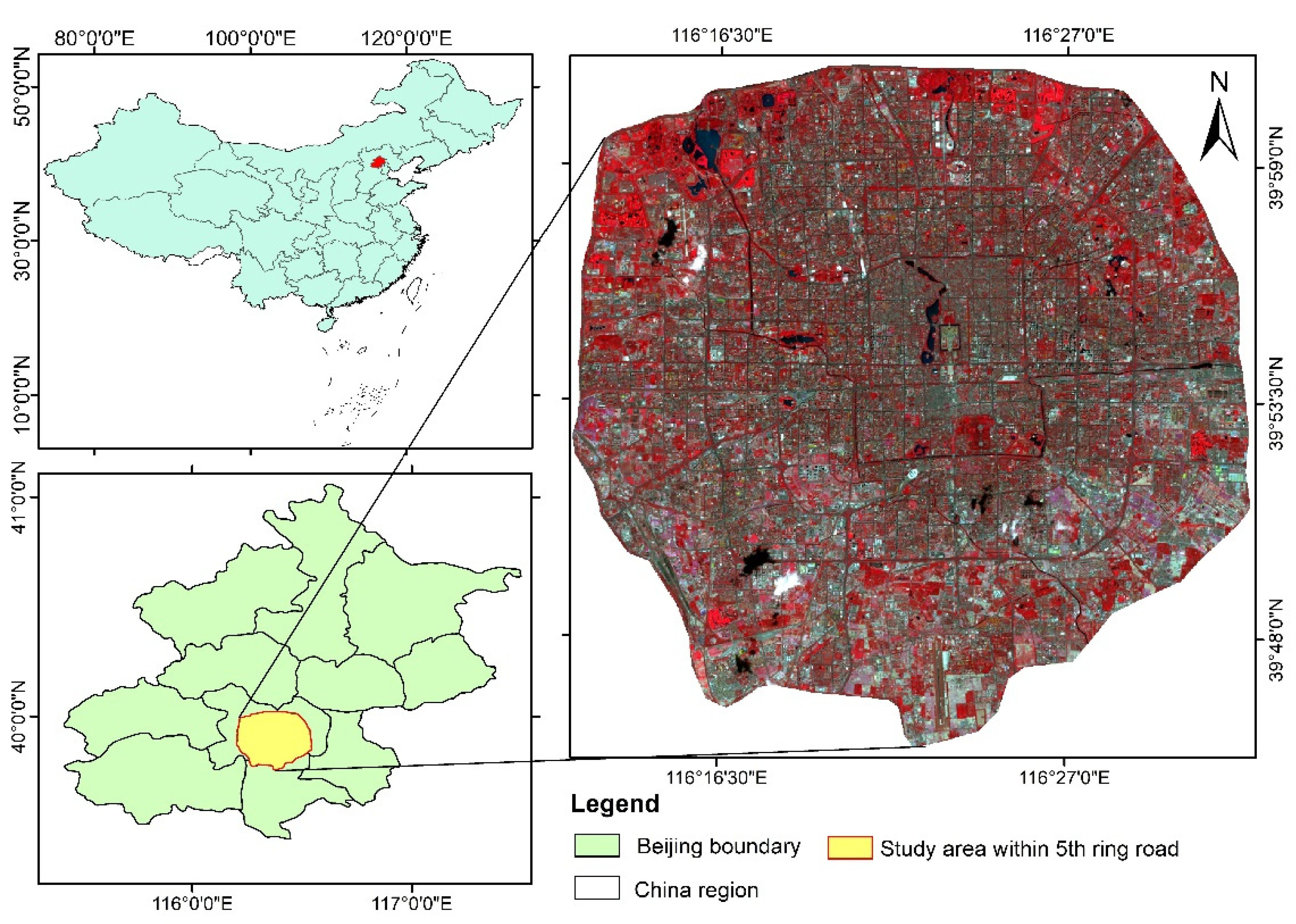
This study focused on the capital city of China, Beijing. The city is located at 39°26′–41°30′ N and 115°25′–117°30′ E, covering about 16,000 km². Additionally, Beijing’s topography is moderately smooth terrain with an elevation range of 20–60 m and small climate variation that does not have a significant influence on surface urban heat islands [7]. The city experiences four seasons and the climate is monsoon-influenced humid continental, with a hot and rainy summer, a cold and dry winter, and short spring and autumn. The current population of Beijing is around 21.54 million. The study focused on the area within the fifth ring road of Beijing, since it is a representative area and the most prosperous part of the city, with concentrated human activity and compact buildings. The geographical location of the study area is depicted in Figure 1.

2.2. Remote Sensing Data

We used high-resolution datasets of the GF-2 satellite for LULC classification, and the Landsat-8 dataset for the retrieval of LST and LULC indices. The LST was retrieved through Split Window (SW) algorithm method, which is applicable and used for reliable LST results [32]. Pre-processing steps were performed before LULC and LST classification, including atmospheric correction (noise and haze), radiometric correction (sun elevation), and an extraction of the interest area. The LULC was classified and mapped from the GF-2 satellite data through the random forest (RF) classifier algorithm [19], and LST was retrieved from Landsat-8 (ETM) by the standard method as suggested in the literature [33,34]. The details of the satellite data are given in

Table 1. Description of the satellite data.

Satellites Scene	Spatial Resolution (m)	Date	Time
GF-2
L1A0002412174		4 June 2017
L1A0002417896		9 June 2017
L1A0002529896		7 August 2017
L1A0002404757	4 × 4	4 June 2017	11:37:47
L1A0002404758		4 June 2017
L1A0002417593		9 June 2017
L1A0002417596		9 June 2017
Landsat-8 ETM	30 × 30	10 July 2017	02:53:19
Thermal Infrared	100 × 100

.

2.3. LULC Classification and Accuracy Assessment

GF-2 satellite images were used for the LULC classification using the RF classifier algorithm by generating different training samples in the form of a polygon representing a homogeneous area of each land cover in ArcMap 10.6. Then, training points were created inside each polygon as a training signature. The GF-2 data and training signatures were processed in R statistical software. Finally, the GF-2 image was classified into five major land cover types (i.e., forest land, built-up area, grassland and agriculture land, barren land, and water bodies). Input sample subsets (sample points) were used to build a tree, and each tree performed a special learning algorithm that split the inputs into subgroups. The trees were grown without pruning and random selection at each node, contrary to a classical decision tree [35]. This process was repeated until the maximum depth was reached or the sample numbers at the node were below the minimum sample threshold. For the LULC classification accuracy assessment, 900 independent systematic sample points were generated at a fixed distance of 0.86 km² in the entire classified map using the Fishnet tool in Arc GIS.10.5. The classification accuracy was checked with the original high resolution unclassified GF-2 image and Google Earth map. LULC classification was achieved with an accuracy of 89% and the kappa coefficient of 0.83 for the city of Beijing, which meets the aim of our research. The validated sample points were further cross-checked against the available detailed LULC maps. The user and producer accuracies were calculated for each land cover class, and Kappa statistics (K) [36] using Equation (1):

K = (observed − expected)/(1 − expected)

(1)

2.4. Land Surface Temperature (LST) Retrieval

LST was retrieved from Landsat-8 (OLI) thermal bands 10 and 11 by using a generalized SW algorithm [32,37], which is extensively applied due to its reliable results [33]. Equation (2) explains the SW algorithm:

$$\mathrm{LST}=T{B}_{10}+C_1\left(T{B}_{10}-T{B}_{11}\right)+C_2{\left(T{B}_{10}-T{B}_{11}\right)}^2+C_O+\left(C_3+C_{4}W\right)\left(1-\varepsilon \right)+\left(C_5+C_{6}W\right)\mathsf{\Delta }\varepsilon$$

(2)

where C₀ (−0.268), C₁ (1.3780), C₂ (0.1830), C₃ (54.30), C₄ (−2.238), C₅ (−1.292), and C₆ (16.40) are the split-window coefficient, TB₁₀, TB₁₁ is the bands brightness temperature in K, ɛ is the mean land surface emissivity of the thermal band, W is the water vapor content in the atmosphere, and Δɛ is the difference in the land surface emissivity of the thermal bands.

2.4.1. Brightness Temperature (TB)

Brightness temperature was calculated from the Top of atmosphere spectral radiance (ToA, $L_{\lambda }$. ToA (A_L)) calculated from multiplicative (0.000342) and additive (0.1) rescaling factors using Equation (3):

$$L_{\lambda }=M_L{Q}_{cal}$$

(3)

Brightness temperature (TB) was obtained by converting thermal digital numbers (DNs) through the process of calibration, and bands 10 and 11 (thermal bands) were used to calculate $T_B$ using Equation (4):

$$TB=\frac{K_2}{L_n{ }_{\left[\left[\frac{K_1}{L_{\lambda }}\right]+1\right]}}$$

(4)

where Qcal is the reflectance of band 10 or 11, M_L indicates the multiplicative rescaling factor, A_L is the additive rescaling factor, and L_λ represents the Top of Atmosphere radiance. Calibration constant K₁ = 774.89 Wm⁻² sr⁻¹ μm⁻¹ and K₂ = 1321.08 K were used in Equation (2) for OLI satellite data.

2.4.2. Land Surface Emissivity (LSE)

To calculate LST, LSE is an important parameter and is quantified by the normalized difference vegetation index (NDVI) threshold method using Equation (5):

$$\mathrm{LSE}={\epsilon }_s(1-\mathrm{FVC})+{\epsilon }_v \mathrm{FVC}$$

(5)

where ${\epsilon }_s (0.971,0.989)$, ${\epsilon }_{v }\left(0.971,0.977\right)$ are the soil and vegetation emissivity of the corresponding thermal bands, and FVC is the vegetation fraction. The algorithms in Equation (6) can calculate FVC:

$$\mathrm{FVC}=( \frac{\mathrm{NDVI}-\mathrm{NDVI}s}{\mathrm{NDVI}v-\mathrm{NDVI}s})$$

(6)

where NDVI = normalized difference vegetation index, NDVIs = NDVI value for soil, and NDVIv = NDVI value for vegetation.

2.4.3. NDVI Threshold

NDVI was calculated from the red and near infra-red bands of Landsat 8-OLI, and FVC was calculated from the classified NDVI values of soil and vegetation. The LSE difference ($\delta \epsilon$) and mean values ($\epsilon$) were calculated using Equations (7) and (8):

$$\epsilon =\frac{{\epsilon }_{10}-{\epsilon }_{11}}{2}$$

(7)

$$\delta \epsilon ={\epsilon }_{10}-{\epsilon }_{11 }$$

(8)

Finally, the LST was calculated in Kelvin by putting the results of Equations (3)–(8) into Equation (2), and then subtracting the value of 273 to convert LST to Celsius (°C).

2.5. Urban LULC Indices Retrieval

Atmospheric and radiometric corrections are very important for indices to avoid errors in the results [17]. The rate of urbanization and urban surface characteristics can be quantified through several LULC indices [28]. The detailed description of LULC indices derived from Landsat-8 (ETM) used to predict LST is given in

Table 2. Various indices and their respective bands are derived from Landsat-8 (OLI).

Index Equation	Bands Wavelength (μm)	Reference
$\mathrm{N}\mathrm{D}\mathrm{V}\mathrm{I}=\frac{\mathrm{N}\mathrm{I}\mathrm{R}+\mathrm{R}\mathrm{E}\mathrm{D}}{\mathrm{N}\mathrm{I}\mathrm{R}+\mathrm{R}\mathrm{E}\mathrm{D}}$	NIR = B5 (0.85–0.88) RED = B4 (0.64–0.67)	[38]
$\mathrm{N}\mathrm{D}\mathrm{W}\mathrm{I}=\frac{\mathrm{N}\mathrm{I}\mathrm{R}-\mathrm{S}\mathrm{W}\mathrm{I}\mathrm{R}1}{\mathrm{N}\mathrm{I}\mathrm{R}+\mathrm{S}\mathrm{W}\mathrm{I}\mathrm{R}1}$	NIR = B5 (0.85–0.88) SWIR1 = B6 (1.57–1.65)	[39]
$\mathrm{N}\mathrm{D}\mathrm{B}\mathrm{I}=\frac{\mathrm{S}\mathrm{W}\mathrm{I}\mathrm{R}1-\mathrm{N}\mathrm{I}\mathrm{R}}{\mathrm{S}\mathrm{W}\mathrm{I}\mathrm{R}1+\mathrm{N}\mathrm{I}\mathrm{R}}$	SWIR1 = B6 (1.57–1.65) NIR = B5 (0.85–0.88)	[40]
$\mathrm{U}\mathrm{I}=\frac{\mathrm{S}\mathrm{W}\mathrm{I}\mathrm{R}2-\mathrm{N}\mathrm{I}\mathrm{R}}{\mathrm{S}\mathrm{W}\mathrm{I}\mathrm{R}2+\mathrm{N}\mathrm{I}\mathrm{R}}$	SWIR2 = B7 (2.11–2.29) NIR = B5 (0.85–0.88)	[41]
$\mathrm{D}\mathrm{B}\mathrm{I}=\frac{\mathrm{B}\mathrm{L}\mathrm{U}\mathrm{E}-\mathrm{T}\mathrm{I}\mathrm{R}1}{\mathrm{B}\mathrm{L}\mathrm{U}\mathrm{E}+\mathrm{T}\mathrm{I}\mathrm{R}1}-\mathrm{N}\mathrm{D}\mathrm{V}\mathrm{I}$	Blue = B2 (0.45–0.51) TIR1 = B10 (10.6–11.19)	[42]
$\mathrm{D}\mathrm{B}\mathrm{S}\mathrm{I}=\frac{\mathrm{S}\mathrm{W}\mathrm{I}\mathrm{R}1-\mathrm{G}\mathrm{R}\mathrm{E}\mathrm{E}\mathrm{N}}{\mathrm{S}\mathrm{W}\mathrm{I}\mathrm{R}1+\mathrm{G}\mathrm{R}\mathrm{E}\mathrm{E}\mathrm{N}}-\mathrm{N}\mathrm{D}\mathrm{V}\mathrm{I}$	SWIRI = B6 (1.57–1.65) Green = B3 (0.53–0.59)	[43]
$\mathrm{N}\mathrm{D}\mathrm{I}\mathrm{S}\mathrm{I}=\frac{\mathrm{T}\mathrm{I}\mathrm{R}1-\left[\frac{\mathrm{M}\mathrm{N}\mathrm{D}\mathrm{W}\mathrm{I}+\mathrm{N}\mathrm{I}\mathrm{R}+\mathrm{S}\mathrm{W}\mathrm{I}\mathrm{R}1}{3}\right]}{\mathrm{T}\mathrm{I}\mathrm{R}1+\left[\frac{\mathrm{M}\mathrm{N}\mathrm{D}\mathrm{W}\mathrm{I}+\mathrm{N}\mathrm{I}\mathrm{R}+\mathrm{S}\mathrm{W}\mathrm{I}\mathrm{R}1}{3}\right]}$ $\mathrm{M}\mathrm{N}\mathrm{D}\mathrm{W}\mathrm{I}=\frac{\mathrm{G}\mathrm{R}\mathrm{E}\mathrm{E}\mathrm{N}-\mathrm{S}\mathrm{W}\mathrm{I}\mathrm{R}1}{\mathrm{G}\mathrm{R}\mathrm{E}\mathrm{E}\mathrm{N}+\mathrm{S}\mathrm{W}\mathrm{I}\mathrm{R}1}-\mathrm{N}\mathrm{D}\mathrm{V}\mathrm{I}$		[43,44]

. The datasets were resampled to the GF-2 resolution before the extraction of pixel values in R statistical software.

NDVI is the difference between near-infrared (which vegetation strongly reflects) and red light (which vegetation absorbs) and ranges from −1 to +1. However, the NDVI ranges vary for each type of land cover and depend on locality. NDVI was derived from the red and near-infrared bands [38], indicated typical LULC types where vegetation is represented by positive values, while negative values indicate built-up areas, barren land, and water bodies [45]. The NDWI is a remote sensing-based indicator sensitive to the water content of vegetation and land surfaces. NDWI is computed using the near-infrared (NIR) and the short-wave infrared (SWIR) reflectance. The NDWI was proposed by [46], and differentiates between liquid and water content due to its sensitivity in the composite landscape [17]. The normalized difference built-up index (NDBI) is a useful measure of the intensity of imperviousness using satellite data and has indices ranging from −1 to 1. The index was proposed for the determination of the built-up area [40]. The UI was first introduced by [41], based on a computer system using Landsat-8 ETM to utilize the brightness relationship of urban areas with the near-infrared and mid-infrared spectrum. The UI is suggested by [28] to identify the LULC from Landsat TM, as an inverse relationship between the brightness of near-infrared and mid-infrared bands. The BSI is proposed by a study [42] for the determination of soil bareness from the inverse modified form of the modified normalized difference water index (MNDWI). The NDISI was used to suppress the vegetation and water bodies and express the impervious surface in the LULC [29]. The threshold value of indices varies from locality to locality. In the previous literature, the relationship between the indices’ actual values and LST was very limited. However, this study focused on the relationship between the actual values of indices and LST discretely and in groups (based on similar characteristics).

2.6. Comparison of LULC, LULC Indices, and LST along the Transects

To obtain an intuitive observation of the LST and LULC indices, four digital line transects [28,47] in the North-South (LT-I), West-East (LT-II), Northwest-Southeast (LT-III), and Northeast-Southwest (LT-IV) directions were used in the urban landscape of Beijing. The directions of the line transect covered the entire LULC, providing maximum information of landscape elements. The value of each pixel along the line transects was obtained based on the resolution of the data. The length of line transects II, III, IV, and I were 33.9, 36.2, 35, and 37.3 km, respectively. We used R Studio software to extract the information of LULC, LULC indices, and LST.

2.7. Statistical Analysis

The relationship between LULC indices and LST was signified through Pearson’s correlation [48]. The linear (univariate), multiple (multivariate) [49], and stepwise regression analyses were performed to optimize LULC indices to predict LST. First, we tested the relationship of each index with LST in linear regression. We examined the NDVI, NDWI in one group, and the NDBI, UI, BSI, DBI, and NDISI in the other group based on the negative/positive effects on LST. The first step was to exclude any multicollinearity effects observed in the form of a high degree of correlation (>0.7) between some of the explanatory variables. For the multivariate regression analysis, we performed a non-multicollinearity test using a package (“GGally”) in R software [50], and removed the indices that had the highest value of correlation (>0.7) between them. The selected indices were systematically tested in R software to remove the multicollinearity based on the criteria used in the previous peer-reviewed literature. Finally, we fitted multiple linear regression models between the non-collinear LULC indices and the response variable (LST) by applying a stepwise regression model using the Akaike information criterion to select the best LULC indices.

2.8. Assessing Temperature Mitigation of Land Cover

In general, the relationship between the percentage of green space, built-up area, and LST was assessed at the city built-up blocks level. The city urban area was divided into major units of 3.6 × 3.6 km within the fifth ring road. The vegetation and impervious surface and its impact on mean LST were quantified in each unit using the zonal statistics tool in Arc GIS 10.6 [51].

3. Results

3.1. Analysis of LULC Types and LST

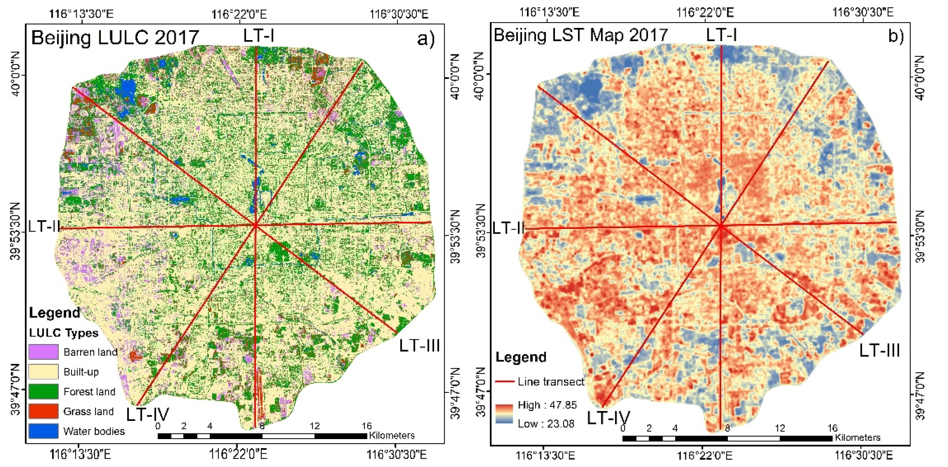
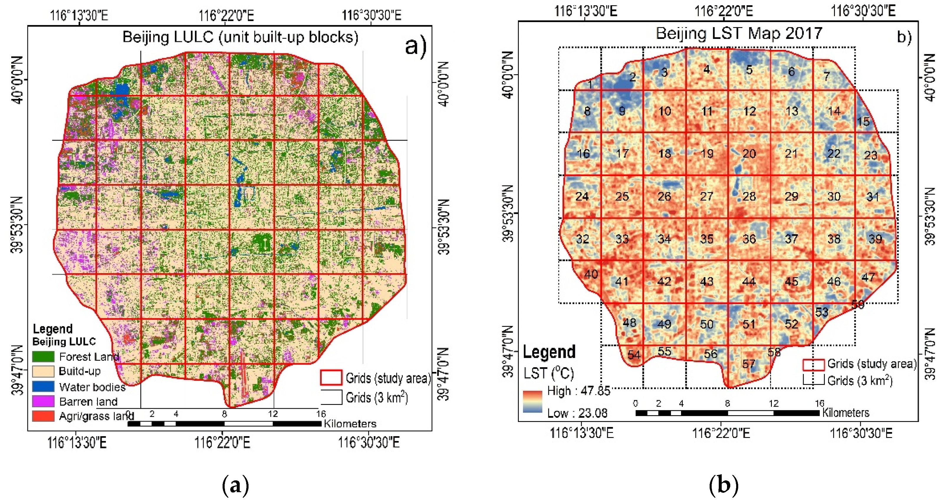
As given in Figure 2, the urban area covered a surface area of 668 km², which is mapped into forest land (24.01%), agriculture and grassland (4.03%), built-up area (63.08%), barren land (7.71%), and water bodies (1.18%). Consequently, the highest mean LST of 37.8 °C was found in the built-up area, followed by 36.61 °C in bare soil, 34.79 °C in agriculture/grassland, 33.64 °C in forest land, and 32.85 °C in water bodies in line transects. Overall, the mean LST pattern was ranked as built-up area > barren land > grass/agriculture land > water bodies > forest land within the fifth ring road of Beijing. The detail of LULC types and their mean LST is depicted in

Table 3. LULC (%) and average LST (°C) of transects.

LULC Types	Forest Land	Built-Up Area	Water Bodies	Barren Land	Grassland	Length/km
LST (LT-I)	30.69	37.58	30.1	36.16	35.14	29
LULC (LT-I)	(24.4%)	(58.2%)	(7.8%)	(6.2%)	(3.3%)	(100%)
LST (LT II)	34.58	38.13	34.88	37.09	36.68	28
LULC (LT II)	(18.8%)	(68.2%)	(0.5%)	(2.5%)	(10%)	(100%)
LST (LT III)	34.6	37.9	32.35	36.42	33.82	31.1
LULC (LT III)	(20.3%)	(62%)	(0.9%)	(9.8%)	(7%)	(100%)
LST (LT IV)	34.67	37.59	34.1	36.76	33.52	31.4
LULC (LT IV)	(17%)	(73.7%)	(1.1%)	(3.8%)	(4.4%)	(100%)
Average LST	33.64	37.8	32.85	36.61	34.79

. Moreover, we quantified the maximum LST difference between built-up area and forest land, followed by forest land and barren land, water bodies, and built-up, respectively. A moderate difference was found between barren and grass/agriculture land, barren land, and built-up area (

Table 4. The LST difference between LULC types.

LULC Types	LST Difference (°C)
Between forest land and built-up	4.16
Between forest land and barren land	2.97
Between water bodies and built up	4.59
Between barren land and grass/Agri land	1.8
Between barren land and built-up	1.19
Between water bodies and forest land	0.79

). Besides, the lowest LST differences were found between water bodies and forest land. Overall, line transect I satisfactorily explained the cooling value of many green patches embedded in the built-up area. The minimum difference in LST values between water bodies and forest land was due to the similar cooling characteristics of the surfaces of land-use types.

3.2. Gradients of LULC Types, NDVI, NDWI, and LST Profile along Transects

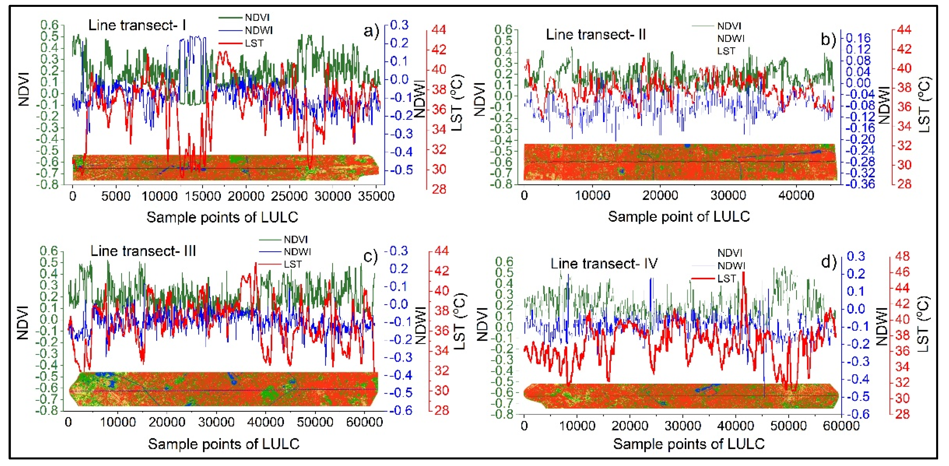
As given in Figure 3, the values of NDVI, NDWI, and LST were found oscillating on LULC types along the line transects. In transect I, the lowest LST was observed with maximum NDVI and NDWI values, while it soared in the built-up area which has the lowest NDVI and NDWI values. In transects III and IV, we observed the highest LST values in the built-up area followed by barren land, and the lowest value in the forest land and water bodies. Due to the maximum area covered by built-up area, the LST fluctuation was minimum along line transect II. Interestingly, in the heterogeneous landscape (shown in Figure 3a,d), the LST and NDVI values showed maximum fluctuation in opposite directions due to the large vegetation patches embedded in the built-up area. The built-up areas distinctly had the highest LST with small NDWI and NDVI values in line transect II. Due to different land surface characteristics, the LST declined sharply in water bodies in line transect I, and small NDVI and NDWI values had elevated LST in the built-up area and barren land (Figure 3c).

3.3. Comparison of LULC Indices and LST in Transects

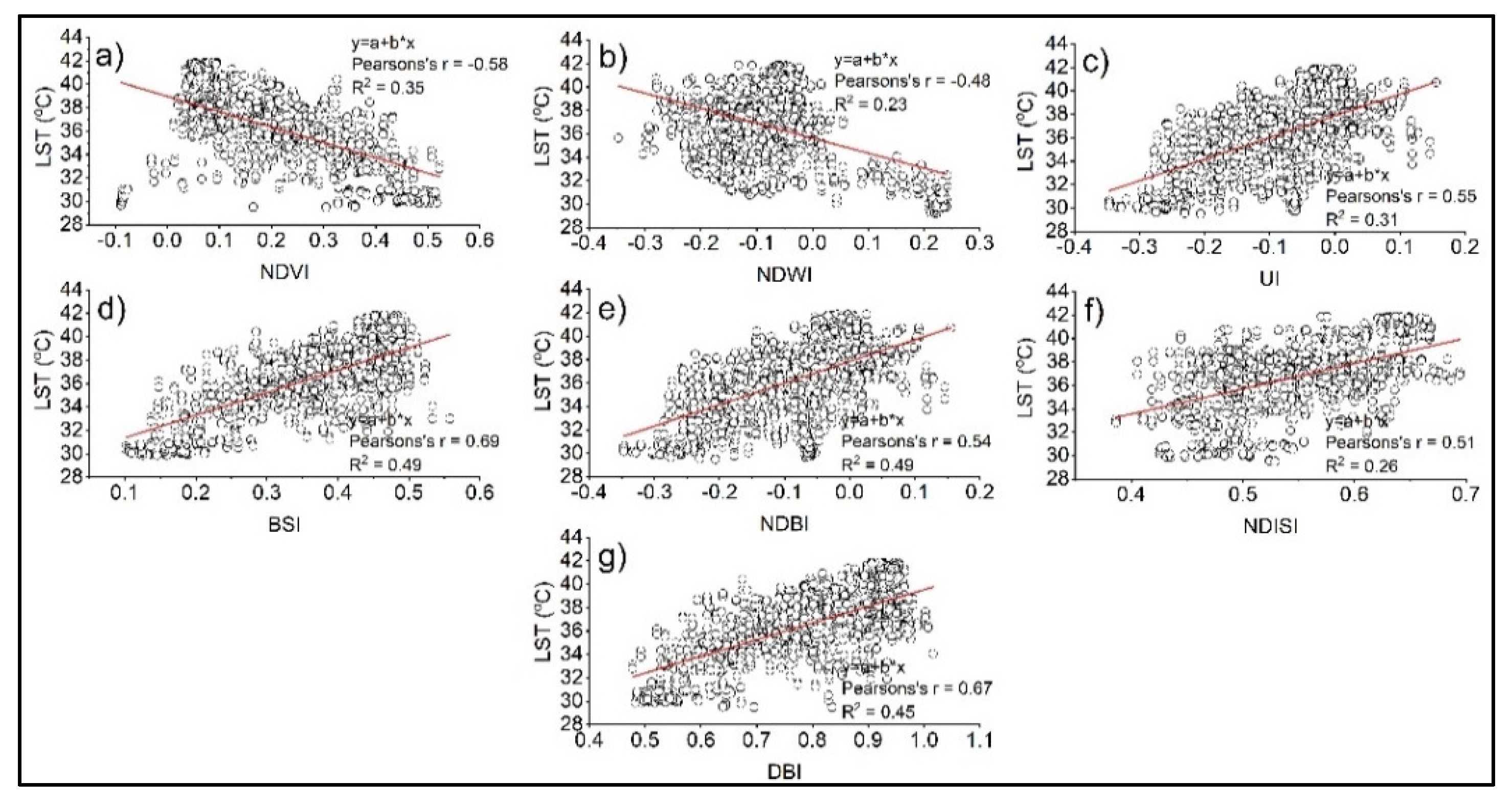
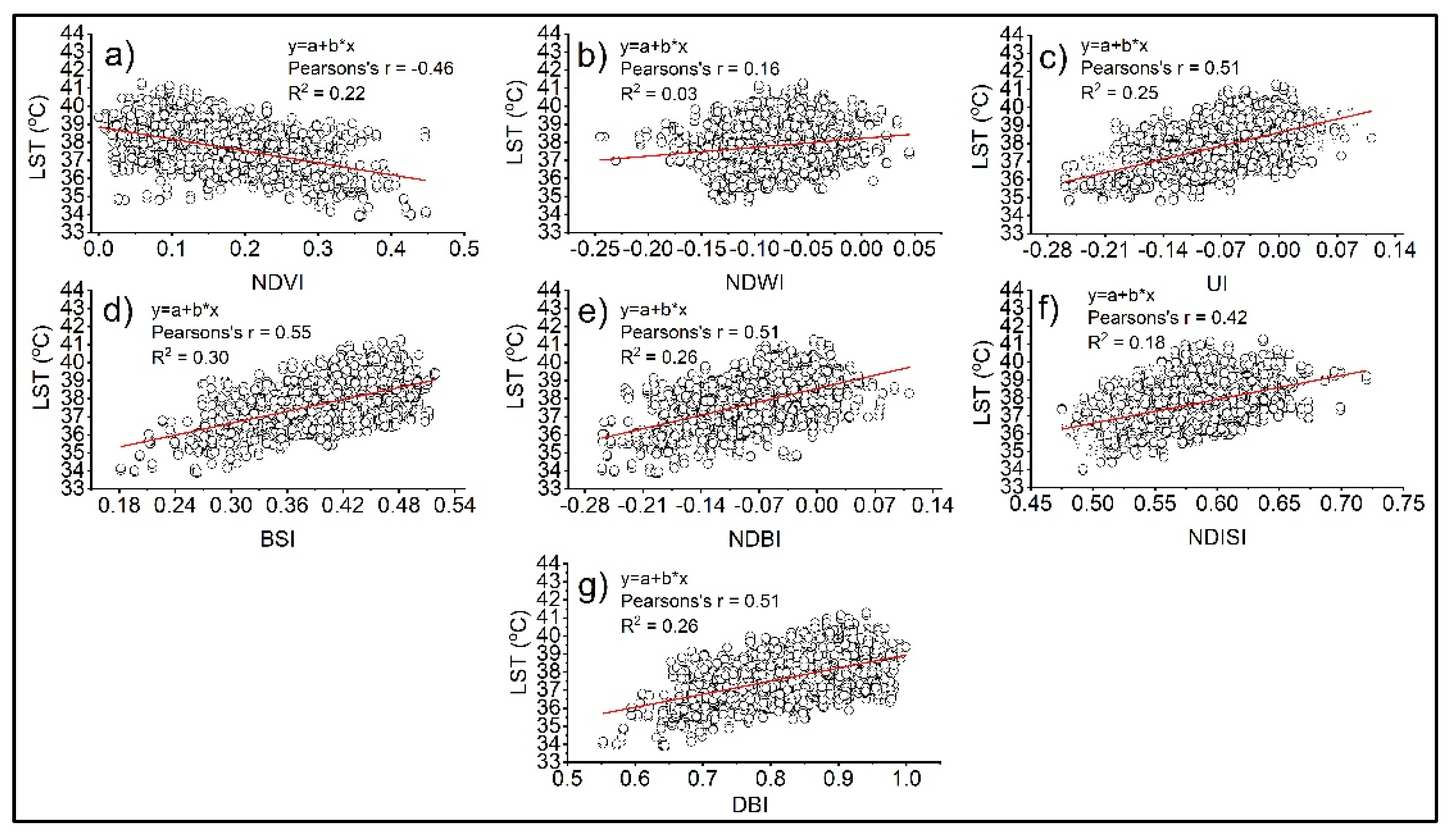
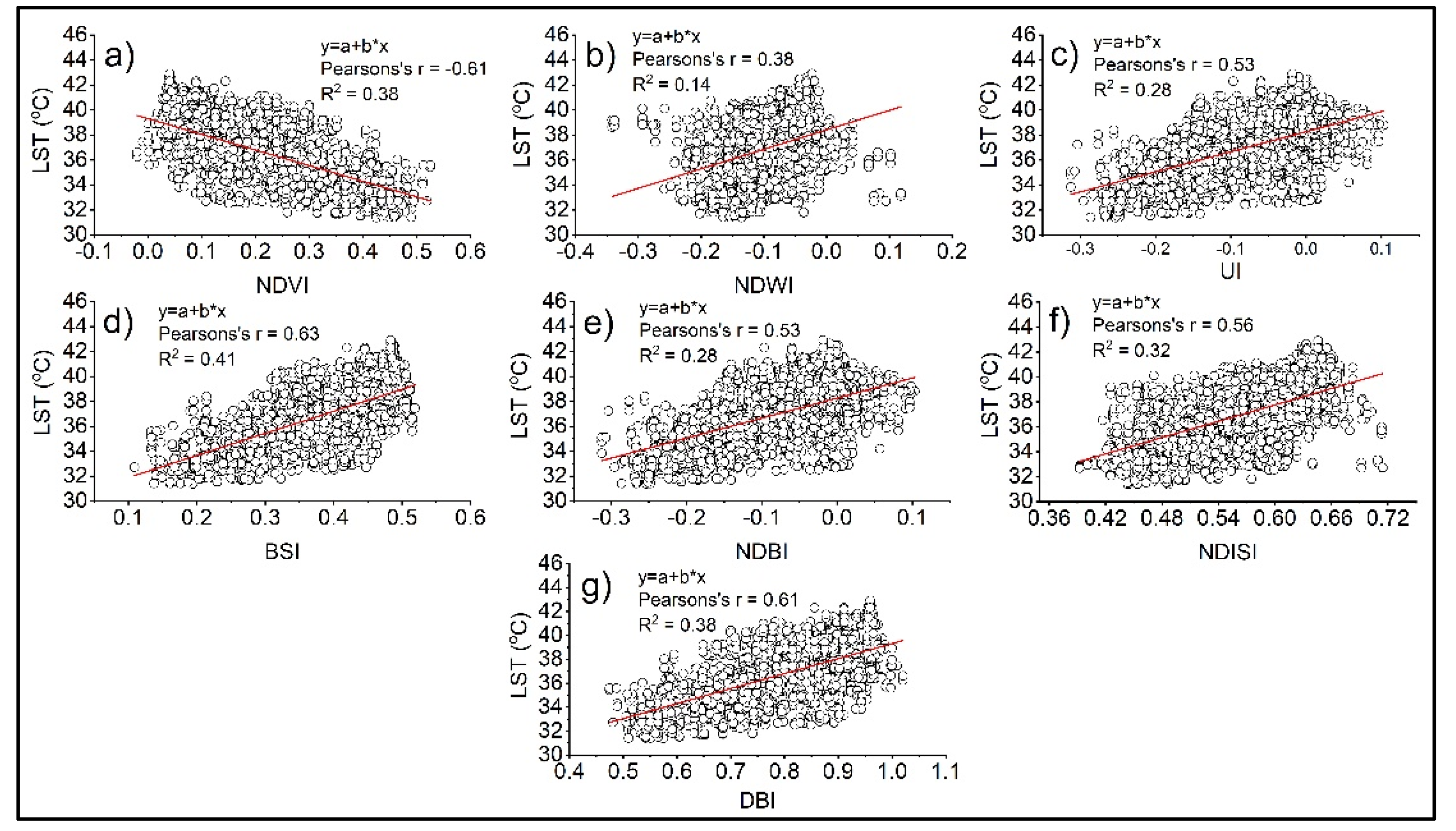
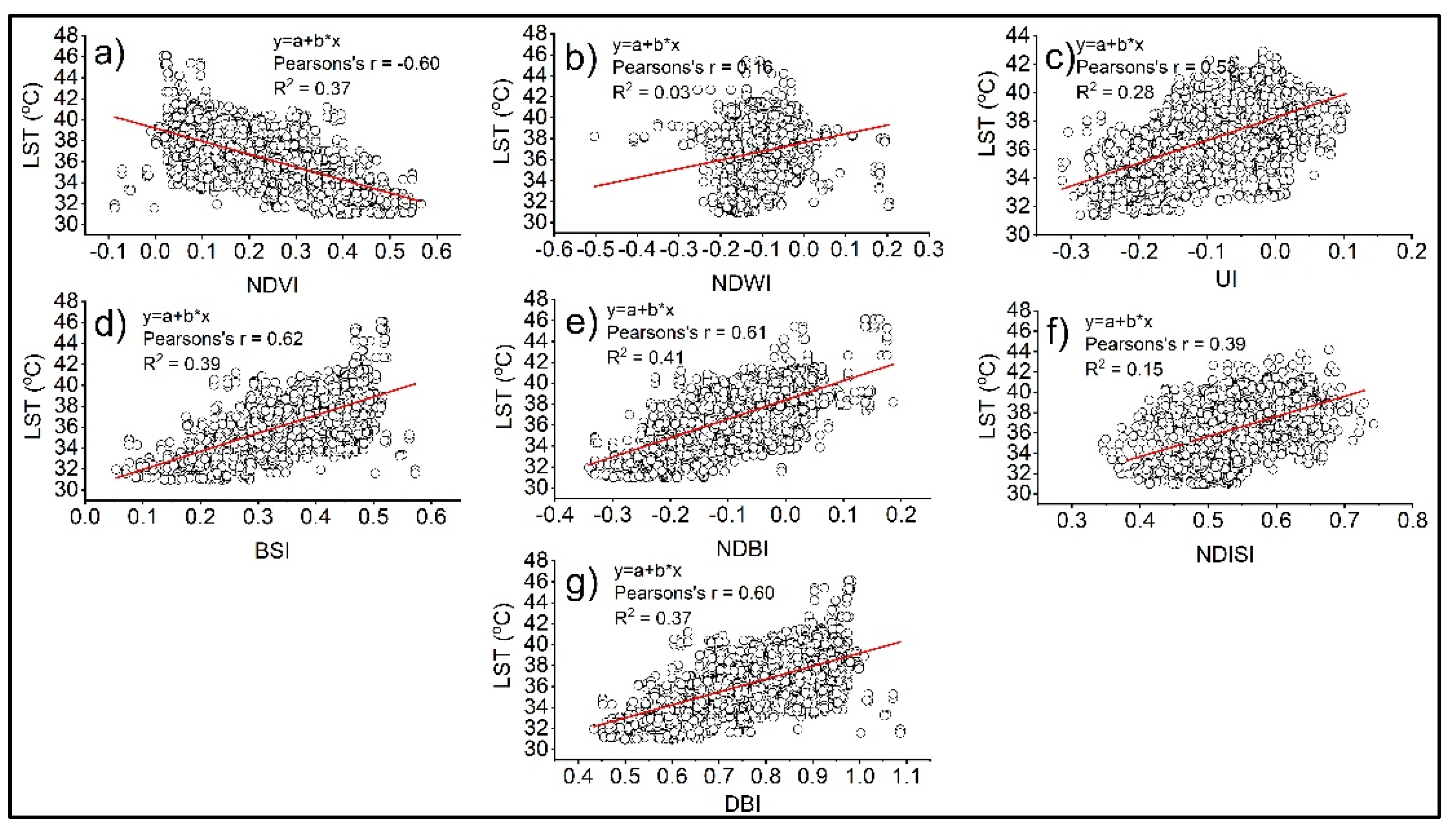
In the univariate analysis, the results showed a negative relationship between NDVI and LST and the analyses of correlation and regression (Pearson’s correlation r = −0.58, R² = 0.35) were satisfactory in line transect I. The downward trend indicated that the decline in LST was due to vegetation pixel along the transects (Figure 4a). In transect II, the relationship between NDVI and LST was slightly significant (Pearson’s r = −0.46, and R² = 0.22), compared to line transect I. The vegetation patches embedded in the built-up area at minimum intervals may be the primary reason for the varied significance level (Figure 5a). In transects III and IV, the correlation and regression analysis between NDVI and LST showed a significant effect (Pearson’s r = −0.61, R² = 0.38) due to the green space cover which had a negative impact on LST compared to line transects I and II (Figure 6a and Figure 7a). Overall, the relationship between vegetation and LST was determinant particularly in transects III and IV. Similarly, water bodies had a strong negative relationship with LST in an urban area. This study found a significant relationship between NDWI and LST in the line transect-I due to the maximum evaporation from water bodies during the hot summer season. In transects II, III, and IV, the analysis found a weak correlation between NDWI and LST due to a minimum number of water pixels. As given in Figure 5b, Figure 6b and Figure 7b, a weak relationship (negligible) between NDWI and LST was found in line transect II, III, and IV. However, in the line transects III and -I the trend is negative, and the variation in the values may be attributed to landscape heterogeneity.

The LULC indices that describe the built-up area and barren land had a relationship between indices and LST. The relationship between the indices such as NDBI, DBI, UI, BSI, and NDISI, and LST was found positive in the univariate analyses along the line transects. In transect I, the analyses of correlation and linear regression between LULC indices and LST were found significant, particularly for BSI (Pearson’s r = 0.72, R² = 0.49) (See Figure 4b). Similarly, the DBI a showed significant result (Pearson’s r = 0.67, R² = 0.45). The other indices had a moderate relationship between NDBI, UI, and NDISI, as given in

Table 5. Parsons’s correlation (r), simple linear regression (R²), and multiple linear regression (MLR) between LST and LULC indices.

LULC Indices	Intercept	Pearson’s r	R2
Line transect I
NDVI	38.97 ± 0.03	−0.58	0.35
NDWI	35.63 ± 0.02	−0.48	0.23
NDBI	37.85 ± 0.01	0.54	0.31
DBI	25.29 ± 0.07	0.67	0.45
UI	37.87 ± 0.017	0.55	0.29
DBSI	29.26 ± 0.11	0.72	0.49
NDISI	24.91 ± 0.14	0.51	0.31
Line transect II
NDVI	38.84 ± 0.01	−0.46	0.22
NDWI	38.21 ± 0.14	0.16	0.02
NDBI	38.56 ± 0.00	0.51	0.26
DBI	31.69 ± 0.05	0.51	0.26
UI	38.61 ± 0.09	0.52	0.25
DBSI	33.35 ± 0.07	0.55	0.3
NDISI	29.89 ± 0.09	0.42	0.18
Line transect III
NDVI	39.31 ± 0.01	−0.61	0.38
NDWI	38.41 ± 0.01	−0.38	0.14
NDBI	38.26 ± 0.10	0.53	0.28
DBI	26.77 ± 0.06	0.61	0.38
UI	38.26 ± 0.10	0.53	0.28
DBSI	26.78 ± 0.06	0.61	0.38
NDISI	24.63 ± 0.07	0.61	0.38
Line transect IV
NDVI	39.20 ± 0.02	−0.6	0.37
NDWI	37.51 ± 0.16	0.2	0.03
NDBI	38.41 ± 0.01	0.61	0.37
DBI	26.85 ± 0.06	0.6	0.37
UI	38.41 ± 0.01	0.61	0.37
DBSI	30.20 ± 0.09	0.62	0.39
NDISI	25.73 ± 0.14	0.49	0.24

. In the line transects, the indices DBI, NDBI, and BSI showed a significant relationship with LST in line transects I, III, and IV, while it was moderate in the line transect II. The correlation between NDVI and LST was strong compared to NDWI due to the maximum vegetation cover than the water along transects.

3.4. Regression Analysis of LULC Indices and LST

In the multivariate analysis, the combined effects of NDWI and NDVI indices on LST were positive but the level of significance was weak compared to the univariate analysis. From the results, we found a moderate relationship (R² = 0.28) between NDWI, NDVI, and LST along line transect I, decreased by a little in transect II (R² = 0.24), and it was found higher in line transects III and IV (R² = 0.39). Overall, the combined effects of NDWI and NDVI were positive in the univariate analysis.

In multivariate analysis, the relationship between the indices, i.e., NDBI, DBI, UI, BSI, NDISI, and LST was found to be positive, implying that these indices might explain LST variation in the line transects in the urban area of Beijing. For instance, the correlation between BSI and LST was significant in the transects II and IV, and a bit lower in the transect I (

Table 6. The multiple linear regression (MLR) between LST and LULC indices.

Various Indices	Co−Efficient	R2	Adjusted R2
Line transect I
Intercept	37.1	0.28	0.28
NDVI	−11.09
NDWI	−15.36
Intercept	45.47	0.26	0.26
BSI	8.27
UI	25.66
DBI	−14.47
NDISI	3.27
Line transect II
Intercept	38.62	0.24	0.24
NDVI	−8.08
NDWI	−5.86
Intercept	37.45	0.31	0.31
NDBI	20.85
BSI	−12.84
NDISI	12.03
Line transect III
Intercept	38.85	0.39	0.39
NDVI	−13.92
NDWI	−6.59
Intercept	29	0.41	41
BSI	16.31
NDISI	2.87
Line transect IV
Intercept	38.85	0.39	0.39
NDVI	−13.92
NDWI	−6.59
Intercept	29	0.4	0.4
BSI	16.31
NDISI	2.87

). The LULC indices such as NDBI, BSI, and NDISI are a predictor of LST after removing the multicollinearity effect in each line transect.

3.5. Stepwise Regression Analysis among LULC Indices and LST

In the stepwise regression analysis, the NDVI, NDWI, and BSI indices in the line transect I, and NDWI, BSI, and NDISI in the line transects II and III, and the NDVI, NDWI, and BSI in line transect IV have a strong relationship with LST after removing the multicollinearity effect. Overall, the selected LULC indices significantly explained the LST in the line transects. The indices explained the LST by 44% except for the NDVI, which has no significant effect in the line transect III, while the indices’ response to LST was 41% in the line transect IV, followed by 34% in line transect I. Among the selected indices, line transect III outperformed to predict LST. The findings indicated that the LULC indices such as BSI, NDISI are the best indicators to explain the LST variation in the heterogeneous urban landscape. The details of the analysis of stepwise regression are given in

Table 7. Significant independent variables in modeling LST during stepwise regression.

Various Indices	Co-Efficient	R2	Adjusted R2
Line transect I
Intercept	31.77	0.34	0.34
NDVI	−6.34
NDWI	−17.57
BSI	10.98
Line transect II
Intercept	25.53	0.32	0.32
NDWI	−13.38
BSI	9.91
NDISI	12.21
Line transect III
Intercept	22.05	0.44	0.44
NDWI	−13.56
BSI	16.64
NDISI	12.73
Line transect IV
Intercept	24.98	0.41	0.41
NDVI	6.16
NDWI	−4.48
BSI	26.89

.

3.6. Impact of Green Landscape on LST at the Built-Up Blocks Level

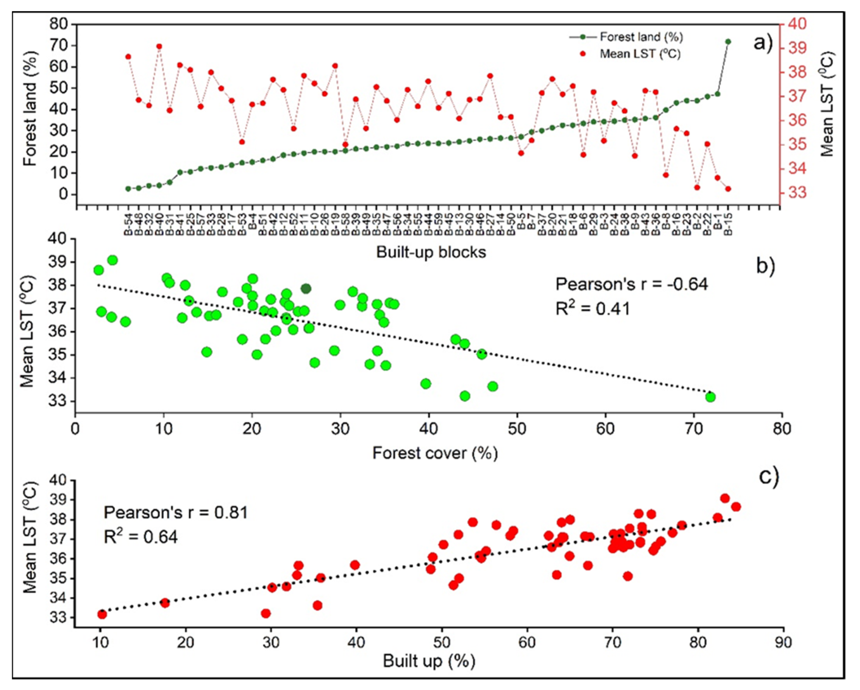
The LULC types significantly contribute to LST, particularly the green spaces and built-up area in the city blocks. As shown in Figure 8a,b, the cooling and warming contribution of the landscape composition, especially the green space and built-up area in each block, was quantified. The analysis of Pearson’s correlation and linear regression indicated a negative relationship between green space and LST at the city-block level (Figure 9b). The vegetation coverage of more than 30% in the built-up blocks had a lower LST value. The analysis of Pearson’s correlation (−0.61) and regression analysis (R²= 0.37), demonstrated that the vegetation influenced the LST of the built-up area in the main urban areas. In addition, the percent cover of built-up in blocks increased the LST compared to other land-use types. For instance, as given in Figure 9c, the trend in Pearson’s and regression analyses showed that the LST significantly correlated (R² = 0.64) with the built-up area in the city blocks. Overall, within the built-up blocks, an average LST difference of about 2–5 °C was observed between the forest land and built-up areas.

4. Discussion

4.1. The Impact of LULC Types on LST

This study aimed to investigate the impact of LULC indices, vegetation, and built-up cover area on LST in the core urban area of Beijing. The city landscape is big, compact, and expanding at an alarming rate. Therefore, the LULC surface characteristics along the line transect method are adequate for making quick decisions. Our results investigated major LULC types in the urban area of Beijing, in which 24.01% was covered by the urban forest and 63.08% by built-up areas in the year 2017. These LULC results are similar to those in the recent literature [32,52], revealing that LULC composition has a great impact on LST and varies according to the spatial pattern of the urban landscape. Our findings on the pattern of mean LST along LULC types is ranked as: built-up > barren land > grass/agriculture land > forest land > water bodies (Table 3). The higher LST in the built-up area followed by barren land is due to the low heat transfer capacity of the surfaces. The land surface temperature is affected by surface characteristics; it is higher in the built-up area and lower in water bodies and vegetation cover of variable density over the land surface, which is inconsistent with the study findings [53]. Similarly, a higher LST in the barren land followed by a built-up area is reported in the city of Islamabad [19].

This study further presented the different LSTs of LULC types. For instance, an LST difference of 4.16 °C was found between the forest land and built-up area, 2.97 °C between the forest land and barren land, and 2.44 °C between the built-up area and water bodies (Table 4). The results confirmed that the forest land and water bodies are important landscape elements, which can co-benefit the urban thermal environment in the hot summer season. Although a proper distribution of water bodies is not possible or cost-effective in urban areas, the next best alternative is the distribution of a sufficient green space, which may lower the LST of the impervious surface and can be applied in each built-up block to serve multiple purposes for urban dwellers, particularly in lowering the land surface temperature.

An early study [17] found a difference of 2–9 °C between water bodies and other land use/land cover types, which confirmed our results. The main reasons for the low LST values of water bodies are due to their high heat transfer capacity and high evaporation rate. Studies have observed that the LST of barren land could have similar or higher values in an urban area [24,54], consistent with our findings. Our study results indicated that the LULC types have different LST values due to their different physical properties and heterogenous landscapes, particularly in compact cities. For instance, evapotranspiration from the green space and water bodies suppresses the land surface temperature, if properly distributed. A study [25] investigated different land use/land cover types along line transects, and agreed with our study findings.

4.2. Contribution of LULC Indices to LST

The present study indicated that the biophysical characteristics (indices) can explain the LST, and a relationship exists between LST and LULC indices. We investigated the pixel values of LULC indices and LST using the line transects method. The study results demonstrate the significant relationship between LULC indices and LST. In univariate analysis, the relationship is negative between LST and NDVI. The pattern of the significance level of NDVI is ranked as line transect III > VI > I > II. It means that the line transect III explained the LST while the lowest level is found in line transect II due to the heterogeneous landscape, which consisted of a more built-up area. The estimated LST of water bodies in combination with vegetation was lower in line transect III. However, water bodies in the urban areas are a special case and have the lowest LST values due to the big water lakes and canals distributed in the city of Beijing, while vegetation tends to have the second-lowest values of LST in an urban area. The vegetation influences LST mainly due to shade and transpiration in the hot summer season.

Similar results are found in an early study [55] that investigated the relationship between NDVI and LST using line transects and noticed a significant correlation coefficient (−0.47). Our findings of line transects III and IV are similar to the mentioned study, and it can be deduced that the correlation is more robust. The variation in the correlation and linear regression values in the line transects is because of the different compositions of landscape elements. The transects covered pixels of different LULC indices, resulting in different significance levels. Likewise, a significant relationship between LULC indices and LST was reported in another study [25], which showed the analysis of correlation in transects. Our results are closely related, but different in the significance levels due to using absolute NDVI values of the typical LULC types. Besides, our findings are still significant with a negative trend line, which might be due to the vegetation in the urban area. The NDWI values are not satisfactory in the line transects except for line transect I.

Furthermore, the relationship between NDVI, NDWI, and LST is slightly significant in multivariate analysis in the line transects compared to univariate analysis. The pattern of the significance level is ranked as transect III > transect I > transect II. The increased significance pattern in the line transect III is due to the combined effect of water bodies and vegetation coverage compared to the line transects II and I. The distribution of large vegetation patches in the built-up area signified the results of line transect III and I, revealing that the combination of blue-green space co-benefited the cooling of the urban climate.

Moreover, the LULC indices (i.e., built-up, bare soil, and barren land) can explain and signify the LST with a positive trend line in univariate and multivariate analyses. Impervious surfaces, dark-colored buildings, and barren land trap the maximum solar energy and contribute to increasing LST in cities. Several LULC indices are used to understand the relationship among the built-up area (NDBI, DBI, UI, NDISI), bare soil (BSI), and LST. Such LULC indices are used to express the characteristics of built-up area, impervious surface, and bare soil surface, particularly the land surface temperature. Our results are significant and positive, particularly between DBI, BSI, and LST in the univariate analysis of the line transects I, III, and IV. In transect II, the significance values of Pearson’s correlation and linear regression are low due to the presence of vegetation patches in the built-up area, which cools down the surface temperature. The significance levels among the indices and LST are weaker in multivariate analysis after performing the non-multicollinearity test.

The collinearity effect is removed and the indices that have a statistically significant effect on LST are selected. It means that the combination of the built-up area and bare soil indices has a great impact on the LST in line transects. For instance, the NDVI and NDWI explained the LST by 28%, 24%, and 39% in line transect-I, II, III and IV, while NDISI and BSI explained the LST by 41% and 40% in the line transects III and IV, respectively. This means that the combined built-up and barren soil-derived indices have a strong relationship with LST. Similarly, a study [56] investigated the relationship of NDBI to LST in the urban area and found a significance value of simple linear regression R² = 0.92. Our results are consistent with this, but the regression value is lower because we consider actual NDBI values of LULC types. In summary, the indices explained the LST along transects, and transect III and IV, in particular, outperformed due to a more heterogeneous landscape. The significant results in the transect III and IV are due to the combined effect of built-up and bare soil indices. Our results of the built-up and bare soil indices and their impact on LST are in close agreement with the findings of the early study [57].

The stepwise regression analysis compared to multivariate analysis explained the LST in the line transects. Overall, the analysis of stepwise regression was slightly significant and predicted the LST by 34%, 32%, 44%, and 41% along transects I, II, III, and IV, respectively. The lowest significance value in transect II is due to the weak performance of BSI compared to other indices. Indeed, the univariate, multivariate, and stepwise regression analyses indicate that the selected indices are acceptable for predicting LST even in the compact urban landscape, i.e., the NDVI has a negative influence on LST, while the built-up and bare soil indices show a positive effect and are good indicators to model LST. Similarly, a study [49] computed five remote sensing indices and found significant results in the univariate and multivariate analyses. These results are significant but slightly different in discussing the positive and negative LST and in the statistical methods they use, highlighting the uniqueness of the present research work.

4.3. Relationship of Green Space to LST and Its Implications

The composition of landscape elements, particularly the green space and built-up space, has a great effect on LST in the city built-up blocks. In this study, the relationship is significant between the green space, built-up space, and LST. The statistical analysis reveals that vegetation is an important urban landscape element that can lower the LST of the urban area. In general, an LST difference of about 1–4.5 °C is investigated between the built-up area and green space in the major built-up blocks (Figure 8b). It is clear that within a unit area of 3.6 km² of the city, vegetation contributed more to the cooling environment in the urban area. The lowest LST was shown with an increased percentage of green space cover within the blocks (Figure 9a). Similarly, we observed that the LST declined as the vegetation cover increased with the decrease in the built-up area. A sharp decline in LST was observed with 30–40% of the green space area in the built-up block, and a further drop-down was observed with the increase in green space percentage. This indicates that Beijing, which has a temperate climate, can decline the LST of the built-up blocks that have least 30–40% of green space cover. Furthermore, there was a negative trend between the percent green space cover and LST. In addition, we observed that the LST values increased with the increase in the built-up cover within the city blocks. These results can be applied to cities that lie in the temperate zone, where at least 30–40% of green space cover is required to cancel the effect of increasing the LST of the impervious surface. Similar results of LST difference between green space and built-up area were found in a study [58] that investigated a difference of 2–5 °C between the built-up area and vegetation cover, and a difference of 2–4 °C was recorded when the impervious surface percentage increased more than 30%. It is worth noting that thermal values are effective in characterizing thermal pattern variability in urban areas, further supporting the findings that the percentage of green space contributes to the urban heat island, thus confirming our results.

5. Conclusions

Investigating the relationship between LULC indices, their impact on LST, and the effects of green space cover unveils useful information for urban managers and designers. This study reported novel findings that LULC has substantial variations in LST values due to the biophysical characteristics of the land surfaces. The line transects approach can be helpful to investigate the LST and land surface for timely decisions. The vegetation and water indices have high negative correlation and may lower the surface temperature. This means that disperse vegetation within the built-up of an urban area at a minimum interval may keep the urban thermal environment cool. Among the indices, NDISI and BSI are preferred to predict LST in a heterogeneous urban landscape. An increase in green space cover can reduce the increasing LST of the built-up blocks, and at least 25–35% can help to mitigate soaring LST in urban areas that lie in the temperate climate zone, like Beijing. Maintaining the composition of green space and impervious cover is integral for ensuring a suitable urban environment. However, the composition of the green space to impervious space may vary in cities belonging to different climate zones. For instance, in tropical cities, at least 50% of the green space could lower the LST, compared to subtropical and temperate regions. Indeed, this study demonstrated the importance of landscape composition and derived RS-based indices in explaining LST in the urban area of Beijing and will provide strong support to select priority measures for future sustainable cities.

Limitations

Some limitations of the study can be identified. First, we only used a single thermal image of one summer season to investigate the surface thermal environment. Second, only the selected LULC indices were used, while there are many other indices that can be used. Third, influencing factors that may affect the LST in the urban areas were not included, such as building height and density, materials used, wind direction, and seasonal variations, all of which are difficult to find in spatial datasets. This study explained the preferred indices that can be used to investigate the urban thermal environment and may provide useful information to urban managers for timely decision-making.

References

- Zhan, W.; Chen, Y.; Zhou, J.; Wang, J.; Liu, W.; Voogt, J.; Zhu, X.; Quan, J.; Li, J. Disaggregation of remotely sensed land surface temperature: Literature survey, taxonomy, issues, and caveats. Remote Sens. Environ. 2013, 131, 119–139. [Google Scholar] [CrossRef]
- Jain, M.; Dimri, A.; Niyogi, D. Land-Air Interactions over Urban-Rural Transects Using Satellite Observations: Analysis over Delhi, India from 1991–2016. Remote Sens. 2017, 9, 1283. [Google Scholar] [CrossRef] [Green Version]
- United Nation. World Urbanization Prospects 2018; UN: New York, NY, USA, 2019; ISBN 9789211483185. [Google Scholar]
- Dickinson, R.E. Land-atmosphere interaction. Rev. Geophys. 1995, 33, 917–922. [Google Scholar] [CrossRef]
- Estoque, R.C.; Murayama, Y.; Myint, S.W. Effects of landscape composition and pattern on land surface temperature: An urban heat island study in the megacities of Southeast Asia. Sci. Total Environ. 2017, 577, 349–359. [Google Scholar] [CrossRef] [PubMed]
- Yu, X.; Guo, X.; Wu, Z. Land Surface Temperature Retrieval from Landsat 8 TIRS—Comparison between Radiative Transfer Equation-Based Method, Split Window Algorithm and Single Channel Method. Remote Sens. 2014, 6, 9829–9852. [Google Scholar] [CrossRef] [Green Version]
- Li, X.; Zhou, W.; Ouyang, Z.; Xu, W.; Zheng, H. Spatial pattern of greenspace affects land surface temperature: Evidence from the heavily urbanized Beijing metropolitan area, China. Landsc. Ecol. 2012, 27, 887–898. [Google Scholar] [CrossRef]
- Barreira, E.; Almeida, R.M.S.F.; Simões, L.M.; Anhas, F. The Importance of Moisture Content to the Emissivity of Ceramic Bricks. Proceedings 2019, 27, 4. [Google Scholar] [CrossRef] [Green Version]
- Rozenstein, O.; Qin, Z.; Derimian, Y.; Karnieli, A. Derivation of land surface temperature for landsat-8 TIRS using a split window algorithm. Sensors 2014, 14, 5768–5780. [Google Scholar] [CrossRef]
- Yu, Y.; Tarpley, D.; Privette, J.L.; Flynn, L.E.; Xu, H.; Chen, M.; Vinnikov, K.Y.; Sun, D.; Tian, Y. Validation of GOES-R satellite land surface temperature algorithm using SURFRAD ground measurements and statistical estimates of error properties. IEEE Trans. Geosci. Remote Sens. 2012, 50, 704–713. [Google Scholar] [CrossRef]
- Brunsell, N.A.; Gillies, R.R. Scale issues in land—Atmosphere interactions: Implications for remote sensing of the surface energy balance. Agric. For. Meteorol. 2003, 117, 203–221. [Google Scholar] [CrossRef]
- Burchard-Levine, V.; Nieto, H.; Riaño, D.; Migliavacca, M.; El-Madany, T.S.; Guzinski, R.; Carrara, A.; Martín, M.P. The effect of pixel heterogeneity for remote sensing based retrievals of evapotranspiration in a semi-arid tree-grass ecosystem. Remote Sens. Environ. 2021, 260. [Google Scholar] [CrossRef]
- Lagouarde, J.P.; Irvine, M.; Dupont, S. Atmospheric turbulence induced errors on measurements of surface temperature from space. Remote Sens. Environ. 2015, 168, 40–53. [Google Scholar] [CrossRef]
- Foley, J.A.; DeFries, R.; Asner, G.P.; Barford, C.; Bonan, G.; Carpenter, S.R.; Chapin, F.S.; Coe, M.T.; Daily, G.C.; Gibbs, H.K.; et al. Global consequences of land use. Science 2005, 309, 570. [Google Scholar] [CrossRef] [PubMed] [Green Version]
- Wu, H.; Ye, L.P.; Shi, W.Z.; Clarke, K.C. Assessing the effects of land use spatial structure on urban heatislands using HJ-1B remote sensing imagery in Wuhan, China. Int. J. Appl. Earth Obs. Geoinf. 2014, 32, 67–78. [Google Scholar] [CrossRef]
- Cai, G.; Du, M.; Xue, Y. Monitoring of urban heat island effect in Beijing combining ASTER and TM data. Int. J. Remote Sens. 2011, 32, 1213–1232. [Google Scholar] [CrossRef]
- Zhang, X.; Estoque, R.C.; Murayama, Y. An urban heat island study in Nanchang City, China based on land surface temperature and social-ecological variables. Sustain. Cities Soc. 2017, 32, 557–568. [Google Scholar] [CrossRef]
- Rehman, A.U.; Ullah, S.; Liu, Q.; Khan, M.S. Comparing different space-borne sensors and methods for the retrieval of land surface temperature. Earth Sci. Inform. 2021, 14, 985–995. [Google Scholar] [CrossRef]
- Khan, M.S.; Ullah, S.; Sun, T.; Rehman, A.U.; Chen, L. Land-use/land-cover changes and its contribution to urban heat Island: A case study of Islamabad, Pakistan. Sustainability 2020, 12, 3861. [Google Scholar] [CrossRef]
- Chen, X.; Zhao, H.; Li, P.; Yin, Z. Remote sensing image-based analysis of the relationship between urban heat island and land use/cover changes. Remote. Sens. Environ. 2006, 104, 133–146. [Google Scholar] [CrossRef]
- Zhang, F.; Tiyip, T.; Kung, H.; Johnson, V.C. Dynamics of land surface temperature (LST) in response to land use and land cover (LULC) changes in the Weigan and Kuqa river. Arab. J. Geosci. 2016, 9, 1–14. [Google Scholar] [CrossRef]
- Sharma, R.; Joshi, P.K. Mapping environmental impacts of rapid urbanization in the National Capital Region of India using remote sensing inputs. Urban Clim. 2016, 15, 70–82. [Google Scholar] [CrossRef]
- Sun, Q.; Wu, Z.; Tan, J. The relationship between land surface temperature and land use/land cover in Guangzhou, China. Environ. Earth Sci. 2012, 65, 1687–1694. [Google Scholar] [CrossRef]
- Song, J.; Du, S.; Feng, X.; Guo, L. The relationships between landscape compositions and land surface temperature: Quantifying their resolution sensitivity with spatial regression models. Landsc. Urban Plan. 2014, 123, 145–157. [Google Scholar] [CrossRef]
- Deng, Y.; Wang, S.; Bai, X.; Tian, Y.; Wu, L.; Xiao, J.; Chen, F.; Qian, Q. Relationship among land surface temperature and LUCC, NDVI in typical karst area. Sci. Rep. 2018, 8, 641. [Google Scholar] [CrossRef] [PubMed]
- Li, J.; Song, C.; Cao, L.; Zhu, F.; Meng, X.; Wu, J. Impacts of landscape structure on surface urban heat islands: A case study of Shanghai, China. Remote Sens. Environ. 2011, 115, 3249–3263. [Google Scholar] [CrossRef]
- Ghosh, A.; Joshi, P.K. Hyperspectral imagery for disaggregation of land surface temperature with selected regression algorithms over different land use land cover scenes. ISPRS J. Photogramm. Remote Sens. 2014, 96, 76–93. [Google Scholar] [CrossRef]
- Xi, Y.; Thinh, N.X.; LI, C. Preliminary comparative assessment of various spectral indices for built-up land derived from Landsat-8 OLI and Sentinel-2A MSI imageries. Eur. J. Remote Sens. 2019, 52, 240–252. [Google Scholar] [CrossRef] [Green Version]
- Sun, Z.; Wang, C.; Guo, H.; Shang, R. A modified normalized difference impervious surface index (MNDISI) for automatic urban mapping from landsat imagery. Remote Sens. 2017, 9, 942. [Google Scholar] [CrossRef] [Green Version]
- Kumar, D.; Shekhar, S. Statistical analysis of land surface temperature-vegetation indexes relationship through thermal remote sensing. Ecotoxicol. Environ. Saf. 2015, 121, 39–44. [Google Scholar] [CrossRef]
- Petropoulos, G.P.; Griffiths, H.M.; Kalivas, D.P. Quantifying spatial and temporal vegetation recovery dynamics following a wildfire event in a Mediterranean landscape using EO data and GIS. Appl. Geogr. 2014, 50, 120–131. [Google Scholar] [CrossRef] [Green Version]
- Naeem, S.; Cao, C.; Qazi, W.A.; Zamani, M.; Wei, C.; Acharya, B.K.; Rehman, A.U. Studying the association between green space characteristics and land surface temperature for sustainable urban environments: An analysis of Beijing and Islamabad. ISPRS Int. J. Geo-Inf. 2018, 7, 38. [Google Scholar] [CrossRef] [Green Version]
- García-Santos, V.; Cuxart, J.; Martínez-Villagrasa, D.; Jiménez, M.A.; Simó, G. Comparison of three methods for estimating land surface temperature from Landsat 8-TIRS Sensor data. Remote Sens. 2018, 10, 1450. [Google Scholar] [CrossRef] [Green Version]
- Wang, Y.; Hu, B.K.H.; Myint, S.W.; Feng, C.; Chow, W.T.L.; Passy, P.F. Science of the Total Environment Patterns of land change and their potential impacts on land surface temperature change in Yangon, Myanmar. Sci. Total Environ. 2018, 643, 738–750. [Google Scholar] [CrossRef]
- Pelletier, C.; Valero, S.; Inglada, J.; Champion, N.; Dedieu, G. Remote Sensing of Environment Assessing the robustness of Random Forests to map land cover with high resolution satellite image time series over large areas. Remote Sens. Environ. 2016, 187, 156–168. [Google Scholar] [CrossRef]
- Stehman, S. Estimating the Kappa Coefficient and its Variance under Stratified Random Sampling. Photogramm. Eng. Remote Sens. 1996, 62, 401–407. [Google Scholar]
- Sobrino, J.A.; Jiménez-muñoz, J.C. Remote Sensing of Environment Minimum con fi guration of thermal infrared bands for land surface temperature and emissivity estimation in the context of potential future missions. Remote Sens. Environ. 2014, 148, 158–167. [Google Scholar] [CrossRef]
- Tucker, C.J. Red and photographic infrared linear combinations for monitoring vegetation. Remote Sens. Environ. 1979, 8, 127–150. [Google Scholar] [CrossRef] [Green Version]
- McFeeters, S.K. The use of the Normalized Difference Water Index (NDWI) in the delineation of open water features. Int. J. Remote Sens. 1996, 17, 1425–1432. [Google Scholar] [CrossRef]
- Zha, Y.; Gao, J.; Ni, S. Use of normalized difference built-up index in automatically mapping urban areas from TM imagery. Int. J. Remote Sens. 2003, 24, 583–594. [Google Scholar] [CrossRef]
- Kawamura, M. Relation between social and environmental conditions in Colombo Sri Lanka and the urban index estimated by satellite remote sensing data. Int. Arch. Photogramm. Remote Sens. 1996, 7, 321–326. [Google Scholar]
- Rasul, A.; Balzter, H.; Ibrahim, G.R.F.; Hameed, H.M.; Wheeler, J.; Adamu, B.; Ibrahim, S.; Najmaddin, P.M. Applying built-up and bare-soil indices from Landsat 8 to cities in dry climates. Land 2018, 7, 81. [Google Scholar] [CrossRef] [Green Version]
- Xu, H. Modification of normalised difference water index (NDWI) to enhance open water features in remotely sensed imagery. Int. J. Remote Sens. 2006, 27, 3025–3033. [Google Scholar] [CrossRef]
- Xu, H. Analysis of impervious surface and its impact on Urban heat environment using the normalized difference impervious surface index (NDISI). Photogramm. Eng. Remote Sens. 2010, 76, 557–565. [Google Scholar] [CrossRef]
- Liu, H.; Weng, Q. Enhancing temporal resolution of satellite imagery for public health studies: A case study of West Nile Virus outbreak in Los Angeles in 2007. Remote Sens. Environ. 2012, 117, 57–71. [Google Scholar] [CrossRef]
- Gao, B.-C. Naval Research Laboratory, 4555 Overlook Ave. Remote Sens. Env. 1996, 7212, 257–266. [Google Scholar] [CrossRef]
- Liu, Y.; Peng, J.; Wang, Y. Diversification of land surface temperature change under urban landscape renewal: A case study in the main city of Shenzhen, China. Remote Sens. 2017, 9, 919. [Google Scholar] [CrossRef] [Green Version]
- Li, Z.L.; Tang, B.H.; Wu, H.; Ren, H.; Yan, G.; Wan, Z.; Trigo, I.F.; Sobrino, J.A. Satellite-derived land surface temperature: Current status and perspectives. Remote Sens. Environ. 2013, 131, 14–37. [Google Scholar] [CrossRef] [Green Version]
- Chen, Y.C.; Chiu, H.W.; Su, Y.F.; Wu, Y.C.; Cheng, K.S. Does urbanization increase diurnal land surface temperature variation? Evidence and implications. Landsc. Urban Plan. 2017, 157, 247–258. [Google Scholar] [CrossRef]
- Ullah, S.; Dees, M.; Datta, P.; Adler, P.; Schardt, M.; Koch, B. Potential of Modern Photogrammetry Versus Airborne Laser Scanning for Estimating Forest Variables in a Mountain Environment. Remote Sens. 2019, 11, 661. [Google Scholar] [CrossRef] [Green Version]
- Ferreira, L.S.; Duarte, D.H.S. Exploring the relationship between urban form, land surface temperature and vegetation indices in a subtropical megacity. Urban Clim. 2019, 27, 105–123. [Google Scholar] [CrossRef]
- Yin, J.; Wu, X.; Shen, M.; Zhang, X.; Zhu, C.; Xiang, H.; Shi, C.; Guo, Z.; Li, C. Impact of urban greenspace spatial pattern on land surface temperature: A case study in Beijing metropolitan area, China. Landsc. Ecol. 2019, 34, 2949–2961. [Google Scholar] [CrossRef]
- Zhang, Y.; Odeh, I.O.A.; Han, C. Bi-temporal characterization of land surface temperature in relation to impervious surface area, NDVI and NDBI, using a sub-pixel image analysis. Int. J. Appl. Earth Obs. Geoinf. 2009, 11, 256–264. [Google Scholar] [CrossRef]
- Ali, J.M.; Marsh, S.H.; Smith, M.J. A comparison between London and Baghdad surface urban heat islands and possible engineering mitigation solutions. Sustain. Cities Soc. 2017, 29, 159–168. [Google Scholar] [CrossRef] [Green Version]
- Kumar, K.S.; Bhaskar, P.U.; Padmakumari, K. Estimation of Land Surface Temperature to Study Urban Heat Island Effect Using Landsat Etm+ Image. Int. J. Eng. Sci. Technol. 2012, 4, 771–778. [Google Scholar]
- Li, H.; Liu, Q. Comparison of NDBI and NDVI as indicators of surface urban heat island effect in MODIS imagery. Int. Conf. Earth Obs. Data Process. Anal. 2008, 7285, 728503. [Google Scholar] [CrossRef]
- Kikon, N.; Singh, P.; Singh, S.K.; Vyas, A. Assessment of urban heat islands (UHI) of Noida City, India using multi-temporal satellite data. Sustain. Cities Soc. 2016, 22, 19–28. [Google Scholar] [CrossRef]
- Liu, K.; Su, H.; Zhang, L.; Yang, H.; Zhang, R.; Li, X. Analysis of the urban heat Island effect in shijiazhuang, China using satellite and airborne data. Remote Sens. 2015, 7, 4804–4833. [Google Scholar] [CrossRef] [Green Version]
Figure 1.
The geographical location of the study area (Beijing).
Figure 2.
(a) LULC of the urban area of Beijing and (b) LST of the study area.
Figure 3.
Relationship among LULC, LST, NDVI, and NDWI profile of (a) line transect I, (b).transect II, (c) line transect III, (d) and line transect IV.
Figure 4.
Relationship between LST and LULC indices in transect I, (a) NDVI, (b) NDWI, (c) UI, (d) BSI, (e) NDBI, (f) NDISI, (g) DBI.
Figure 5.
Relationship between LST and LULC indices in transect II, (a) NDVI, (b) NDWI, (c) UI, (d) BSI, (e) NDBI, (f) NDISI, (g) DBI.
Figure 6.
Relationship between LST and LULC indices in transect III (a) NDVI, (b) NDWI, (c) UI, (d) BSI, (e) NDBI, (f) NDISI, (g) DBI.
Figure 7.
Relationship between LST and LULC indices in transect IV (a) NDVI, (b) NDWI, (c) UI, (d) BSI, (e) NDBI, (f) NDISI, (g) DBI.
Figure 8.
Relationship between (a) LULC, and (b) LST within the built-up area.
Figure 9.
Relationship between forest and LST, (a) relationship between forest land (%) and LST, (b) regression analysis between forest and LST, (c) regression analysis between built-up and LST.