Article

Spatial Distribution of Precise Suitability of Plantation: A Case Study of Main Coniferous Forests in Hubei Province, China

1
Key Laboratory of National Forestry and Grassland Administration on Ecological Landscaping of Challenging Urban Sites, National Innovation Alliance of National Forestry and Grassland Administration on Afforestation and Landscaping of Challenging Urban Sites, Shanghai Engineering Research Center of Landscaping on Challenging Urban Sites, Shanghai Academy of Landscape Architecture Science and Planning, Shanghai 200232, China
2
Beijing Engineering Research Center of Soil and Water Conservation, Beijing Forestry University, Beijing 100083, China
3
Lab of Urban Design and Science, New York University Shanghai, 1555 Central Avenue, Shanghai 200122, China
4
Shanghai Foundation Ding Environmental Technology Company, Shanghai 200063, China
5
College of Electronic and Information Engineering, Shanghai Dianji University, Shanghai 201306, China
*
Author to whom correspondence should be addressed.
Land 2022, 11(5), 690; https://doi.org/10.3390/land11050690
Submission received: 7 April 2022 / Revised: 18 April 2022 / Accepted: 1 May 2022 / Published: 5 May 2022

Abstract

:
(1) Background. Conifers are the main plantation species in southern China, including Masson Pine (MP), Chinese fir (CF) and Chinese thuja (CT). Clarifying the suitable site conditions for these conifers is helpful for large-area afforestation, so as to manage forests to provide a higher level of ecosystem services. To achieve the research goals, we take the conifers in Hubei Province of southern China as a case study. (2) Methods. The situations of conifers, as well as environmental conditions of 448 sampling plots, were then investigated. The suitable growth environment of conifers in the studied area was determined by the maximum entropy algorithm, and the suitability spatial distribution of coniferous forests at the provincial level was also analyzed. (3) Results. The effect of the conifers suitability prediction model reached an accurate level, where AUC values of MP, CF and CT training set were 0.828, 0.856 and 0.970, respectively. Among multiple environmental factors, such as geography and climate, altitude is the most important factor affecting conifer growth. The contribution of altitude to the growth suitability of MP, CF and CT was 38.1%, 36.2% and 36.1%, respectively. Suitable areas of MP, CF and CT were 97,400 ha, 74,300 ha and 39,900 ha, accounting for 52.45%, 39.97% and 21.46% of the studied area, respectively. We concluded that the suitable site conditions of conifer plantations were 2800–5600 °C annual accumulated temperature, 40–1680 m a.s.l., and <40° slopes. (4) Conclusions. The study suggests that accurate spatial suitability evaluation should be carried out to provide sufficient support for the large-area afforestation in southern China. However, due to our data and study area limitations, further studies are needed to explore the above findings for a full set of plantation species in an extensive area of southern China.

1. Introduction

Plantations play an important role in global forest resources. They can not only provide wood supply resources, but also promote ecological restoration, landscape reconstruction and environmental improvement [1,2]. However, the sustainable management of plantations is facing difficulties [3]. In the middle reaches of the Yangtze River, due to inappropriate site conditions and poor species spatial structure, the vegetation growth trend and the ecological function of plantations are poor, resulting in a series of problems such as soil erosion and biodiversity decline [4,5,6]. There are many factors that affect the growth quality of plantations [7]. Whether the environmental conditions are suitable for plants is not considered, and large areas of plantation forests will lead to factors such as light, temperature, water and fertility that do not meet the needs of plant species [8].
Since the 1980s, countries around the world have developed plantations for different purposes, such as industrial timber forests and ecological public welfare forests, through artificial afforestation or reforestation, so that the area and volume of plantations in the world show a growing trend [6,9]. In 2020, the world’s plantation area was 293.9 million ha, and the growth rate was 1.10% (2010–2020) [10]. China’s plantation area ranks first in the world. In 2020, the plantation area was 84.70 million ha, accounting for more than one-third of the national forest area, with an annual growth rate of 1.45% (2010–2020) [10]. The development process of plantations in China is typical and representative, which has important reference and enlightenment significance for the construction and maintenance of plantations in the world [11,12].
Since the 19th century, many scholars have found that species diversity, vegetation growth, and productivity of plantation forests have decreased significantly due to environmental degradation, especially soil degradation [6,13]. The suitability of species site conditions for species refers to whether the climatic conditions, geographical conditions, and other conditions of a certain region are suitable for its growth [14,15]. The analysis of the suitability of species site conditions is not comprehensive enough to achieve the suitability of land and species, which is one of the main reasons for the degradation of the ecological function of plantations [16,17]. Therefore, the suitability of plant species, the relationship between geographical distribution and climate, and the simulation and prediction of geographical spatial distribution are carried out [18,19]. Plant suitability analysis is one of the key research hotspots in global ecology and global change biology, which has important theoretical and practical significance [20]. Based on this requirement, many different statistical methods came into being, and species distribution models (SDMs) have been produced one after another [21,22]. Species distribution models mainly use the distribution data of species and environmental data to correlate, predict the niche of species according to the algorithm, reflect the preference of species for habitat with entropy, and explain the habitat suitability of species [23]. There are many studies on species suitability. At present, it is widely used in habitat prediction of rare, endangered, and economic species [24], the distribution of invasive species and propagation prediction of diseases and insect pests [25,26,27,28], screening of priority reserves [29,30], the impact of climate change on species distribution, etc. [31,32,33].
The species distribution models were developed in the 1980s. It was initially a conceptual analysis model based on the existing data on species distribution. Common models were models based on environmental thresholds and distance thresholds to predict species distribution, such as the Bioclim classic framework model established in 1986 [34]. The habitat model was based on biological characteristics [35], and the classification confidence Domain model was based on Diva-GIS software [36]. The Garp model was implemented by a genetic algorithm [37], the artificial neural network (ANN) model was established by a distributed mathematical–statistical model [38,39], and the maximum entropy algorithm (MaxEnt), which calculates entropy, was based on an unbiased estimation [40,41,42]. In the later stages, with the progress of technology and the increase in available data types, the species distribution model gradually developed into a statistical model based on applied classification and discriminant analysis. The use of data types was also more abundant, mainly including the Biomod model [43], the generalized linear model (GLM) based on normal linear generalization [44], and a more flexible nonparametric extended generalized additive model (GAM) [45,46].
With the continuous development of the species distribution model, the research on plantation species suitability was also deepening, and the model and technical methods gradually matured [47]; Kabir et al. (2005) took Eucalyptus camaldulensis, Acacia mangium and other species in the Dhaka forests of Bangladesh as a research object, and found the optimal analysis model suitable for each species by comparing seven regression analysis models [48]. Kimsey et al. (2008) took Abies in the northern Edwards region of the United States as a research object, and calculated its site index by using a geographically weighted regression model, analyzing and evaluating the site index of Abies. When evaluating the suitability of Acacia species [49], Wang et al. (2002) combined the GIS analysis method with the economic management decision support (EMDS) model to divide the suitability of Acacia in the study area into three levels [50]. Among the different models, MaxEnt belongs to its learning model, which finds the geographical location of suitable target species by finding the geographical distribution with the maximum entropy [51]. The MaxEnt still has good prediction accuracy under less data demand, and the model is suitable for global regions. In addition, it has a higher tolerance to data deviation problems because of small samples and irregular sampling, and it has excellent prediction performance.
Hubei Province is located in the middle of the Yangtze River Basin in China. The area of coniferous forest accounts for 55% of the total forest land [52]. Its reasonable forest management plays an important role in improving the ecological function of coniferous forests. In past afforestation, the analysis of species suitability was not accurate enough to achieve the right place and species, which degraded the ecological function of coniferous forests [53]. The objectives are as follows, to: (1) explore the method of accurate suitability evaluation of plantation growth; (2) identify the site factors affecting the growth of coniferous forest in the study area; and (3) obtain the area and spatial distribution position of the suitable growth area of coniferous forests. Based on a large amount of sample data, the interpolation model and species distribution model were used to improve the prediction accuracy. The results can provide important theoretical support and technical reference for the improvement and transformation of the construction of plantations and ecological function.

2. Materials and Methods
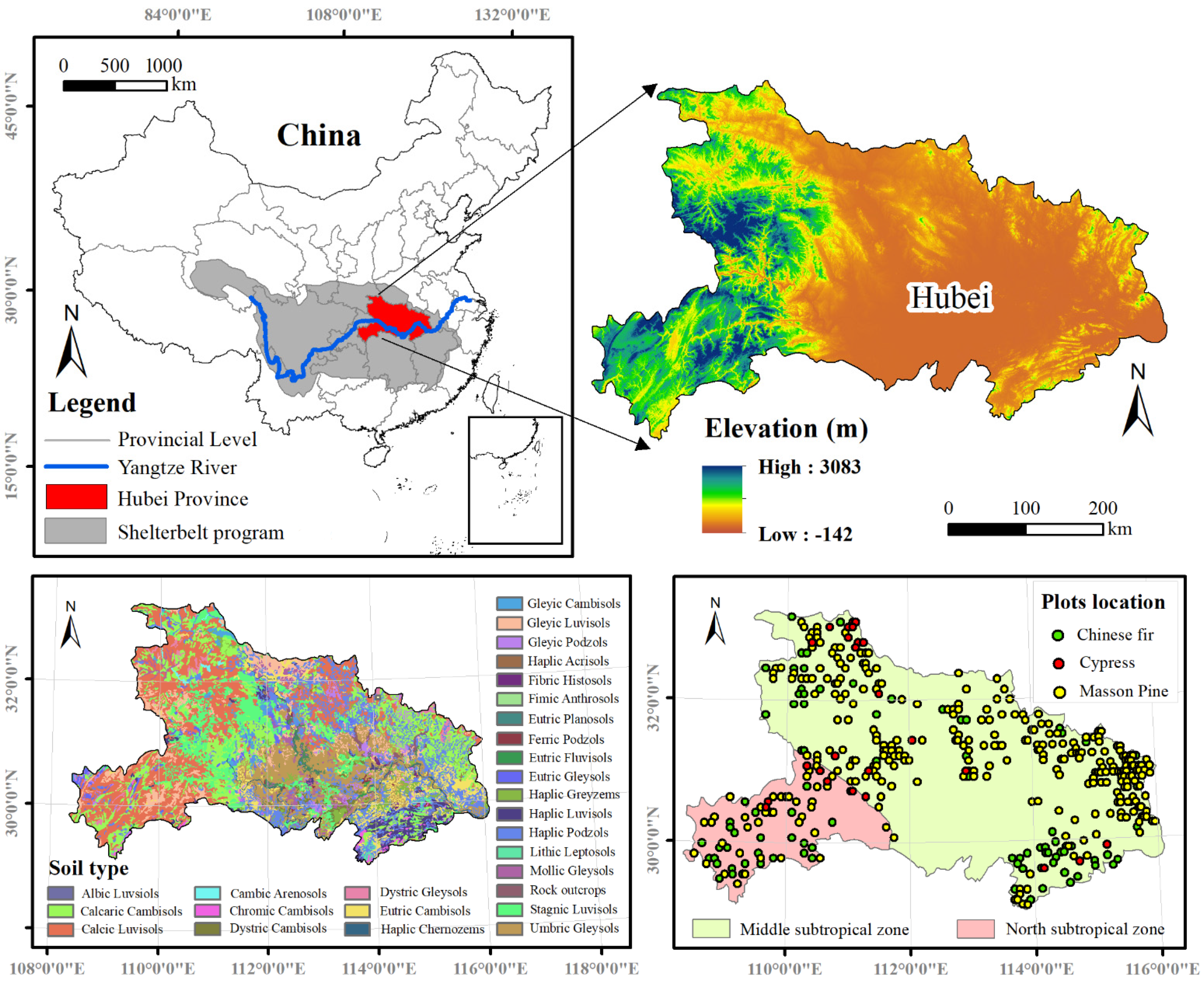
2.1. Study Area

Hubei province (latitude of 29°01’53″–33°6′47″ N and longitude of 108°21′42″–116°07′50″ E) is located in the middle reaches of the Yangtze River, covering an area of 185,900 km2 (Figure 1). The study area is located in the subtropical monsoon climate area, which makes this area hot and rainy in summer and cold and dry in winter [54]. The forestland area in the province is 7.9389 million ha, accounting for 42.71% of the total land area. It is mainly distributed in mountainous and hilly areas, and less in plain areas. The forest species are also dominated by artificial forest species such as Masson pine (Pinus massoniana), Chinese fir (Cunninghamia lanceolata) and Chinese thuja (Platycladus orientalis).
According to the topographic characteristics, such as altitude, slope and aspect, the data of plantation sample points are evenly selected for investigation and mining in Hubei Province. The plantation height, diameter at breast height (DBH), canopy density, total vegetation coverage, litter thickness, community structure, plantation species structure, volume, longitude and latitude and other information were recorded. The data of 467 plantation plots (20 × 20 m2) were obtained, including 294 Masson Pine (MP) plots, 105 Chinese fir (CF) plots and 68 Chinese thuja (CT) plots.

2.2. Data and Method

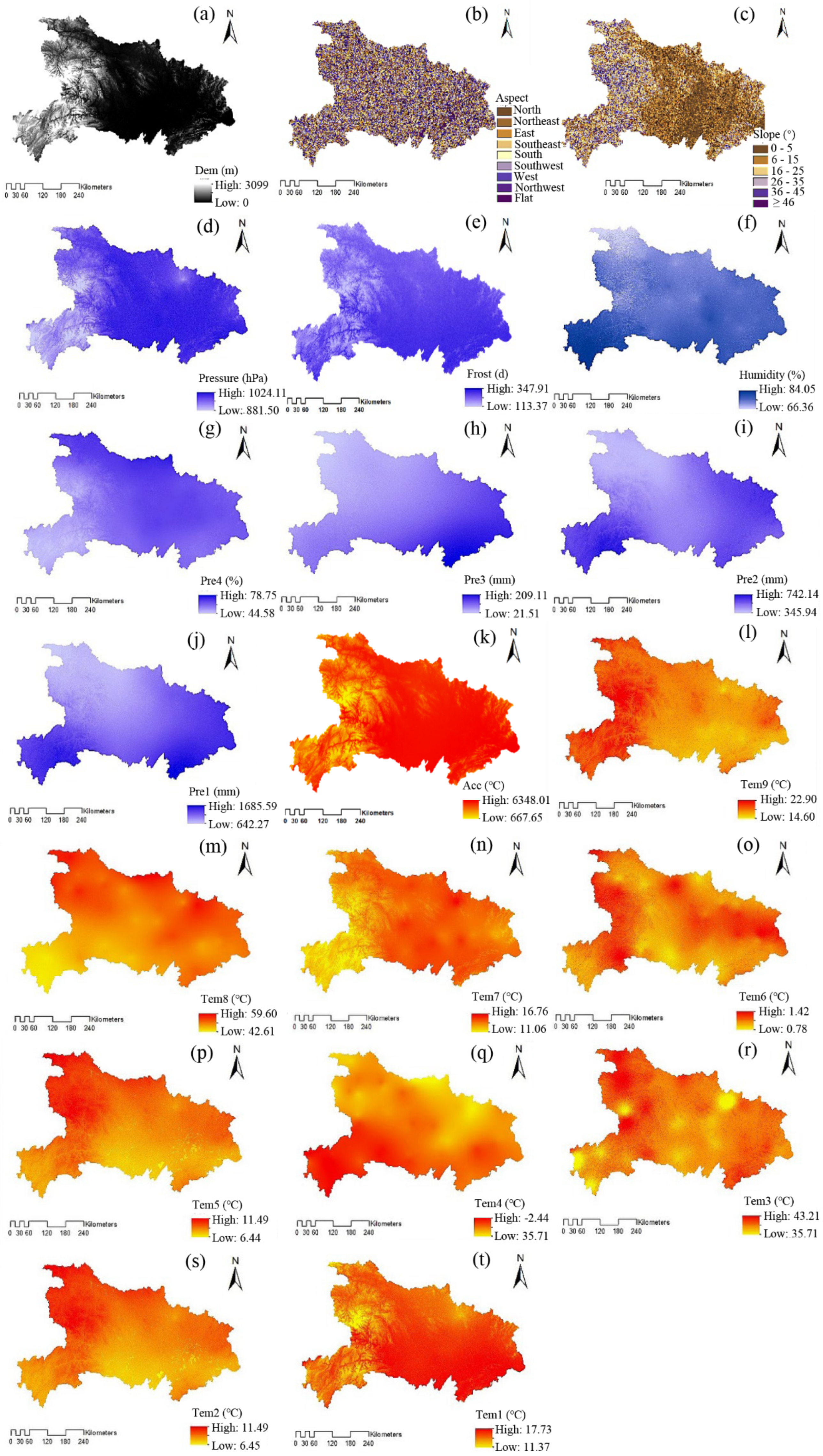
2.2.1. Data Acquisition

The meteorological data come from the cumulative monthly and monthly data of China’s surface from 1981 to 2010 on the Chinese Meteorological Science Data Center (http://data.cma.cn/, accessed on 1 May 2022). It contains the data of 103 meteorological stations (67 in Hubei Province and 36 outside neighboring provinces). The data include temperature, precipitation and three other types (Table 1). The air temperature data include nine air temperature elements: mean temperature, average annual temperature difference between day and night, the highest temperature in the hottest month, the lowest temperature in the coldest month, annual temperature daily range, minimum temperature daily range, standard deviation of air temperature, annual temperature range and isotherm; the precipitation data include annual rainfall, rainfall in the wettest season, rainfall in the driest month and relative standard deviation of rainfall; other data include air pressure and humidity Shape data coming from digital elevation data (DEM) of geospatial data cloud (https://www.gscloud.cn/, accessed on 1 May 2022). The slope, aspect and altitude data are calculated from DEM data. The soil data are from the big data center of sciences in cold and arid regions (http://bdc.casnw.net/yyzc/sj/250299.shtml, accessed on 1 May 2022).

2.2.2. Data Processing

Multiple Linear Regression Kriging (MLRK) was used to interpolate and calculate meteorological station data in different climate zones (Figure A1) to obtain continuous meteorological spatial distribution data. This method is more accurate than the data measured by meteorological stations. In the process of meteorological data interpolation, the normalized data such as altitude, slope and aspect are used as auxiliary variables; stepwise regression method is used to screen and regression fitting is carried out to calculate the residual of multiple linear regression at a meteorological station location, and the ordinary Kriging method is used to interpolate the residual of regression. The predicted value of each point was obtained by adding the determined part and residual interpolation result of each predicted point [55]. The formula is as follows:
Z ^ ( s 0 ) = k = 0 ρ β ^ k q k ( s 0 ) + i = 1 n λ i e ( s i )
where Z ^ ( s 0 ) is the interpolation result of predicted position points, and k = 0 ρ β ^ k q k ( s 0 ) is the deterministic part of regression fitting. Ei-A,e (s) is the interpolation result part of ordinary Kriging on regression residual; K represents the position serial number during regression fitting; β represents the total number of spatial positions; β ^ k is the coefficient of regression model; β ^ 0 is the intercept when k = 0 ; i represents the position sequence of regression residual interpolation, n represents the total number of spatial positions; q k ( s 0 ) is the value of an auxiliary variable of predicted position points; λ i is the weight of ordinary Kriging interpolation determined by the spatial correlation structure of regression residual, and e(si) is the residual at position s i .

2.3. Ecological Function Evaluation of the Sample Land

There are good and bad ecological quality samples in the survey sample plot, so good samples need to be screened as data for suitability evaluation. The ecological function of the sample plot refers to the method proposed in the technical regulations on continuous inventory of national forest resources formulated by the China Forestry Administration in 2004 [56]. The index mainly includes eight indexes: forest volume, naturalness, average stand height, canopy density, total vegetation coverage, litter thickness, community structure and species structure, which can comprehensively evaluate the growth of species. Table A1 and Table A2 are the classification criteria and basis of the ecological index. The calculation method of the ecological function index is as follows:
K = 1   W i X i
where K is the ecological index, Xi represents the result of the ith evaluation factor (grade I, grade II and grade III), and Wi represents the weight of each evaluation factor. The sample plots with ecological function grades I and II are determined to be suitable for the growth of coniferous trees. A total of 448 sample plots suitable for coniferous growth (including 291 MPdata, 95 CFdata and 62 CT data were used as supporting data for scientific evaluation of coniferous forest suitability.

2.4. Space Suitability Division

According to the ecological suitability of the species, the geographical factors were treated in a unified coordinate system. Firstly, the restricted geographical elements are used for spatial superposition to eliminate unsuitable areas (divided according to experience). Then the suitability index of each grid is calculated by using the MaxEnt in the possible suitable area. Finally, the suitability is classified according to the suitability index and its accuracy is evaluated.

2.4.1. Space Suitable for Unit Screening

According to the relevant literature, the suitable spatial units are roughly divided according to the suitable growth environment of species [57], and the formula is as follows:
SRi = Temi × Prei × Soii × DEMi
where i stands for the ith pixel. SRi refers to the appropriate spatial unit of the coniferous trees. When SRi = 1, it means that the grid position is suitable for conifer growth in theory, and when SRi = 0, it means that the grid position is not suitable. Temi represents annual average temperature; Prei represents annual precipitation; DEMi represents altitude; and Soii represents soil types.

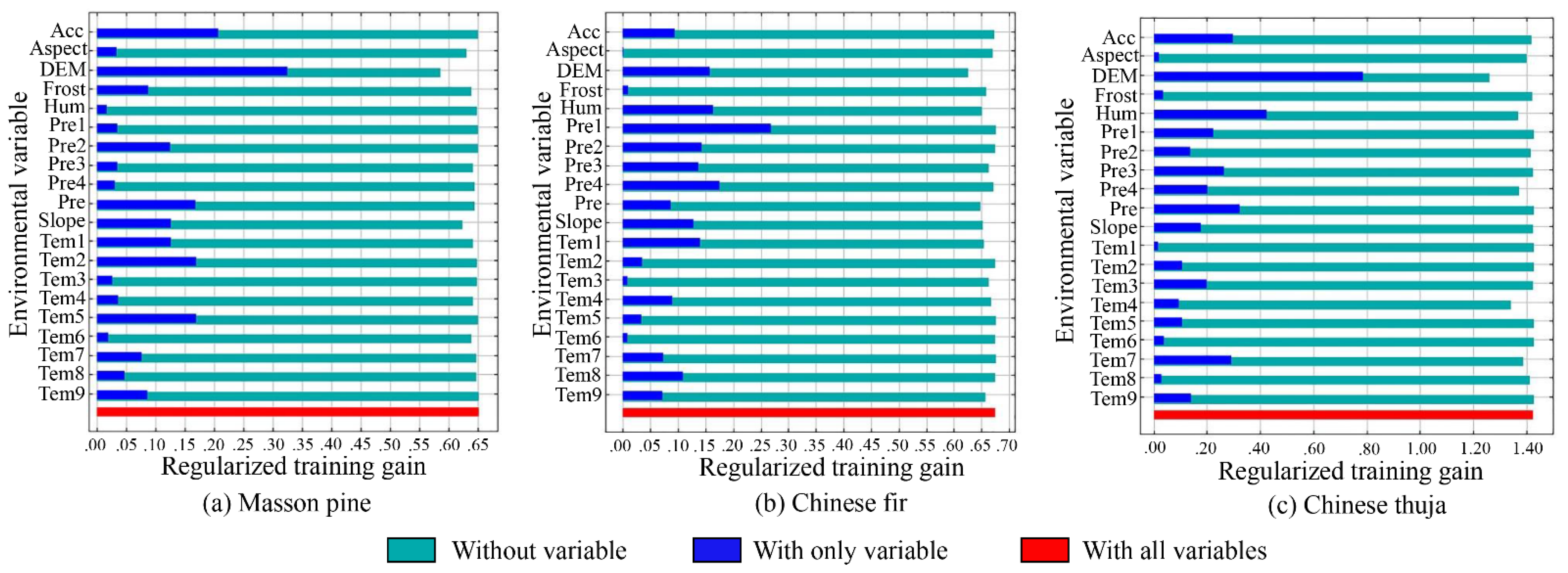
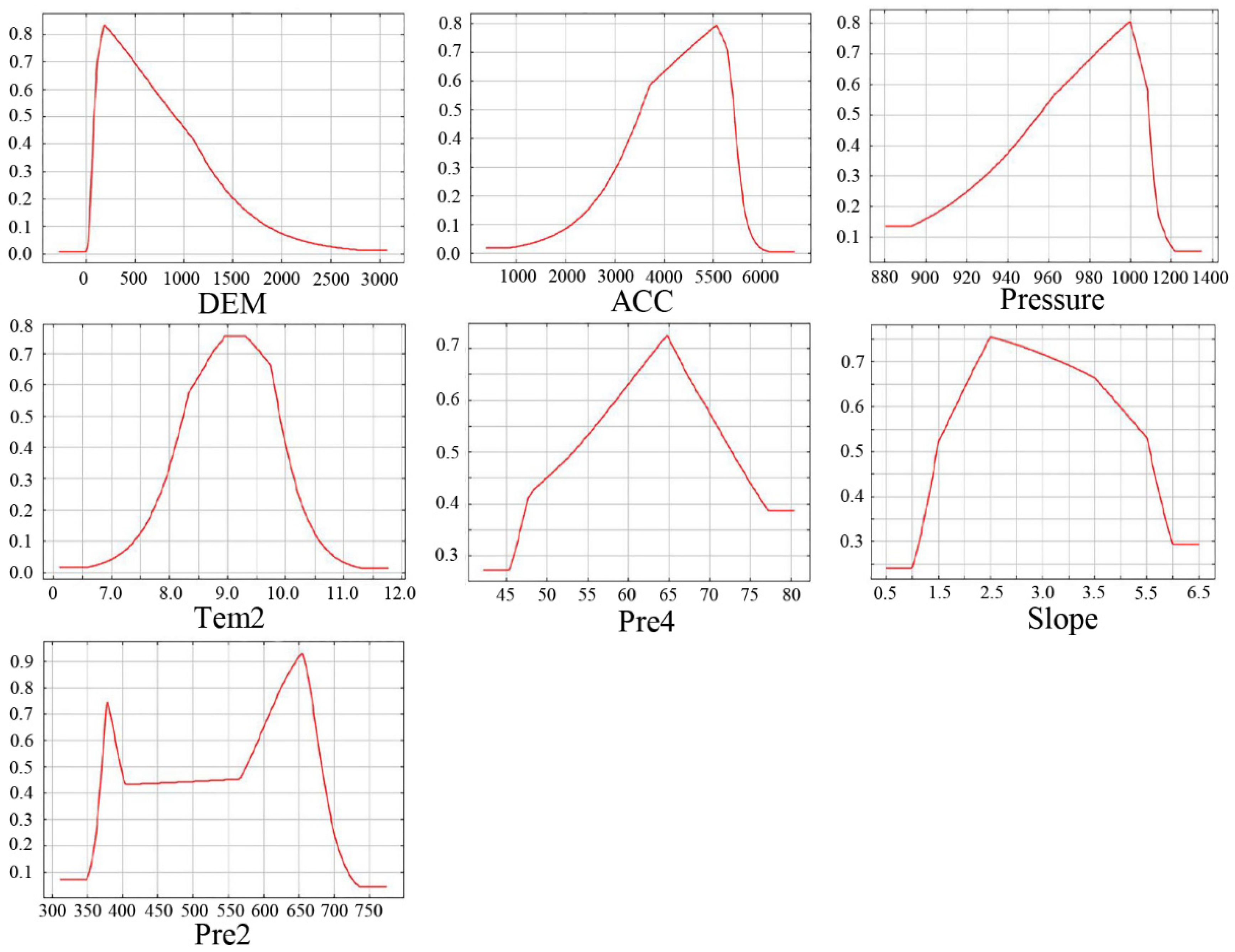
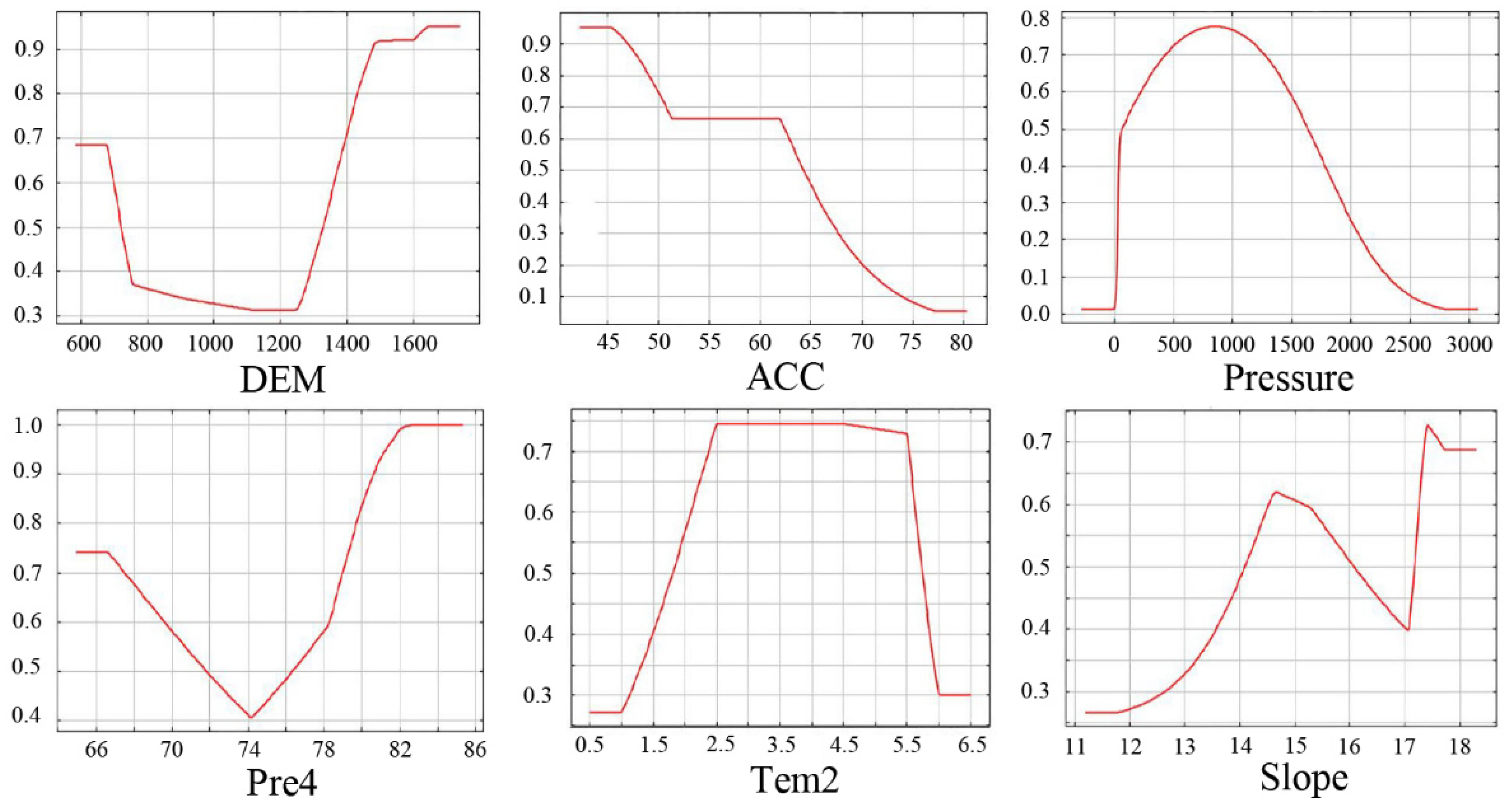
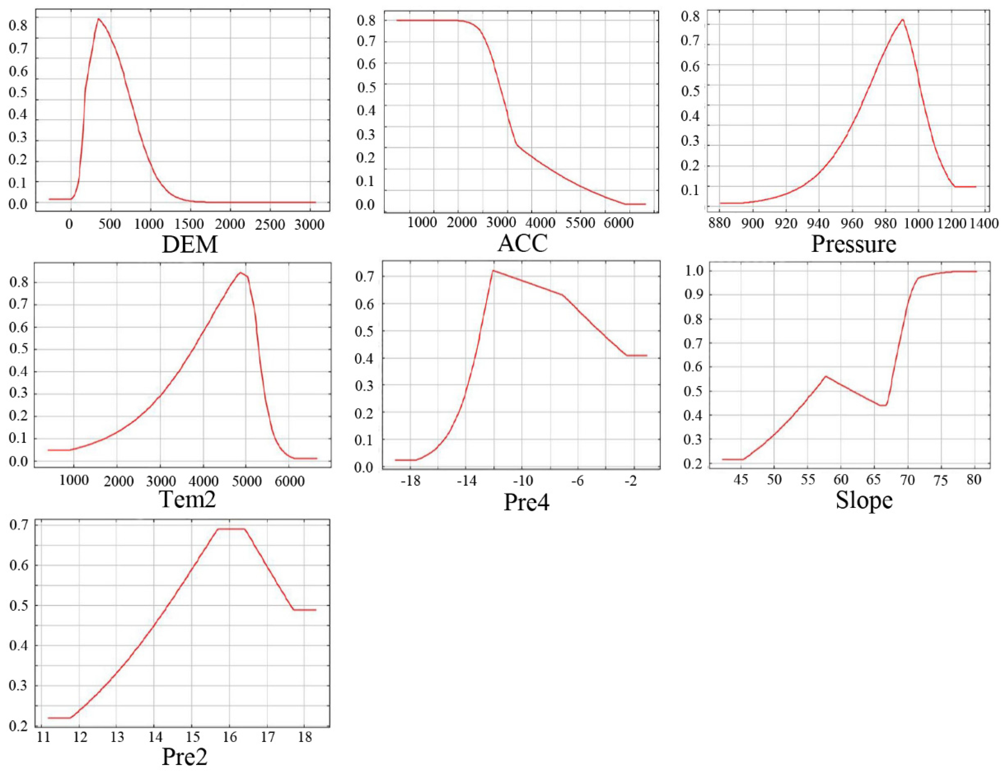
2.4.2. Filtering of Potential Distribution Key Environment Variables

There are many environmental factors affecting species distribution, including climate factors, soil factors, vegetation distribution and so on [58]. We selected 24 environmental variables to build the initial model. The jackknife test in MaxEnt software was selected to determine the contribution of environmental variables to the model prediction, and eliminate the environmental variables with a small contribution based on the test results.

2.4.3. MaxEnt Model

MaxEnt model does not make any biased assumptions about the unknown when the known conditions are met, so the prediction risk of the model is the smallest (http://www.cs.princeton.edu/, accessed on 1 May 2022, Version 3.4.1). The formula is:
maxH ( Y / X ) = i j p ( x I i , y j ) l o g p ( y j / x i )
where X { x 1 , x 2 , , x n } , Y { y 1 , y 2 , , y n } are discrete variables. In the calculation, the model calculates the constraint conditions of target species distribution according to the environmental characteristic variables of species quadrat data, explores the possible distribution of maximum entropy under this constraint, and predicts the habitat distribution and suitability of target species in the study area [59]. The output result of the MaxEnt model is 0–1. The larger the value, the greater the distribution probability of species. In this study, 25% of the distribution data is randomly selected as the testing date, and the remaining 75% is used as the training data. The contribution of each environment variable to coniferous forest data distribution is determined by a jackknife test. According to the distribution probability (P) and the fitness grade of coniferous trees in the study area, P < 0.05 is the non-fitness area, 0.05 ≤ P < 0.2 is the low fitness area, 0.2 ≤ P < 0.5 is the medium fitness area, and 0.5 ≤ P ≤ 1 is the high fitness area.

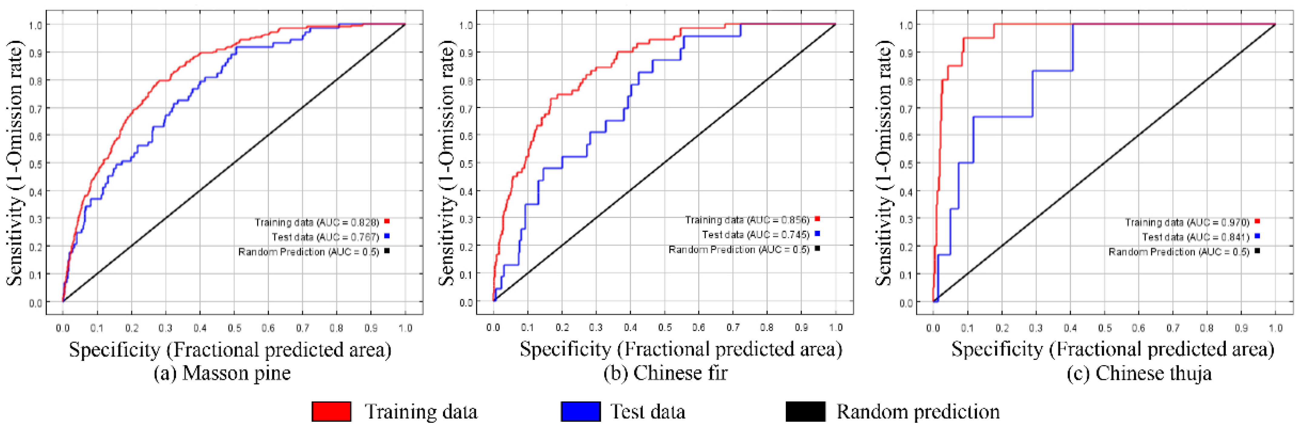
2.5. Validation of Model Accuracy

In this study, the area under the curve (AUC) under the receiver operating characteristic curve (ROC curve) was used as the criterion to evaluate the model simulation results (He et al., 2021). ROC curve, also known as sensitivity curve, is drawn with the false-positive rate (1-specific rate) and true-positive rate (1-missing rate) as abscissa and ordinate, respectively, according to a series of different two classification methods. The area value under the curve is the AUC value, with a value range of 0 to 1. The closer the AUC value is to 1, the greater the correlation between environmental variables and distribution models, and the higher the accuracy of prediction results (Table 2).

3. Results

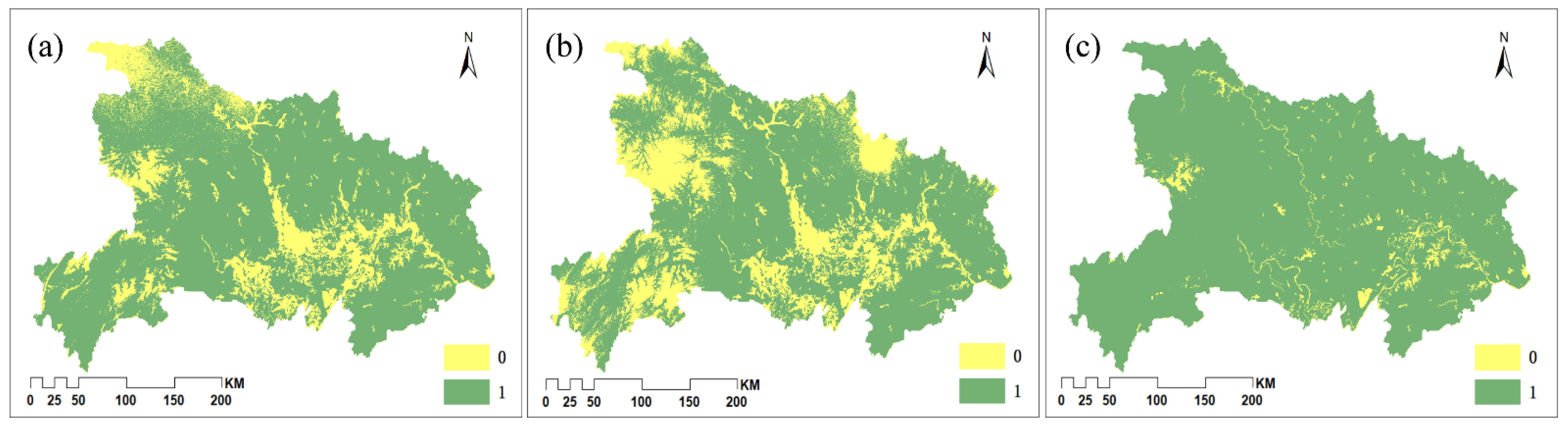
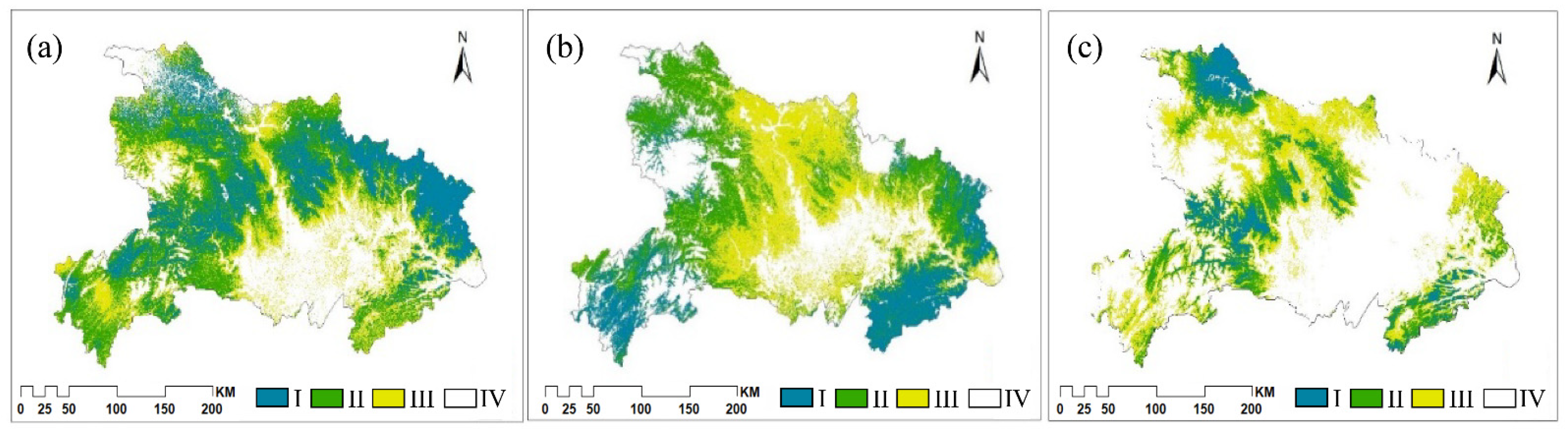
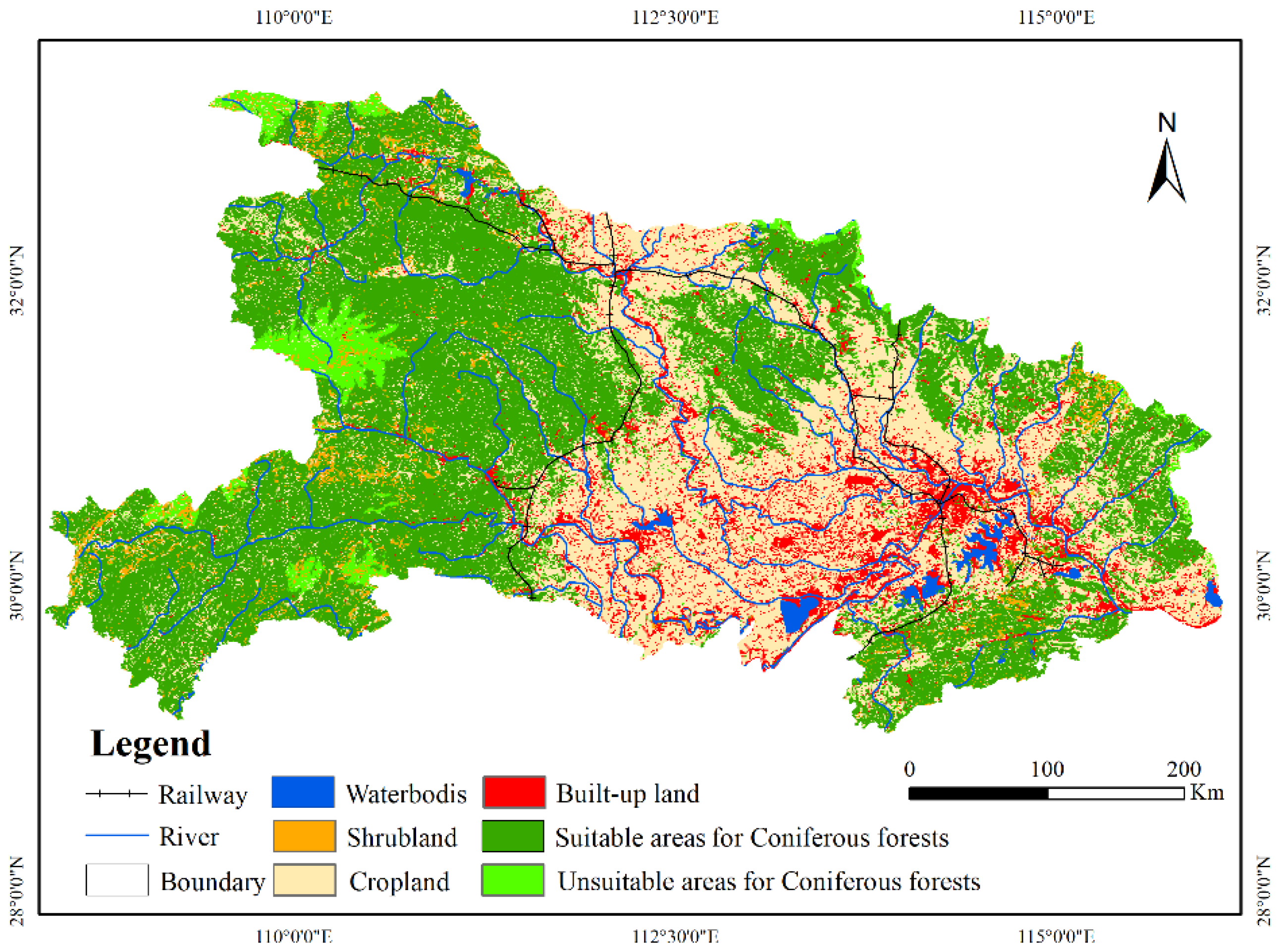
3.1. Spatial Distribution of Main Coniferous Forests

The division of possible suitable units was based on the mastery of the basic habits of the target species, and the spatial areas in the area that were not suitable for plant growth were preliminarily excluded through environmental factors. The target species of this study were MP, CF and CT. MP was a positive species, suitable for the annual average temperature of 13–22 °C, the annual precipitation of 800–1800 mm, the altitude of less than 1500 m, the soil requirements were not strict, suitable for slightly acidic soil, and not suitable for swamp soil, meadow soil or wetland. CF was suitable for an annual average temperature of 15–23 °C, annual precipitation of 800–2000 mm and altitude of less than 1200 m. It was not suitable for swamp soil, meadow soil or alkaline soil. CT was suitable for the annual average temperature of 13–19 °C, the annual precipitation was higher than 1000 mm and the altitude was lower than 2000 m. It was not suitable for swamp soil, meadow soil or alkaline soil (Figure 2).

3.2. Evolution Characteristics of Landscape Patterns of LUCC

For MP, the top five factors in order of importance were altitude, accumulated temperature, air pressure, mean diurnal range and poor annual temperature, among which altitude contributes the most to its distribution, and the score of individual training score was more than 0.3 (Figure 3). For CF, the top five factors were annual rainfall, rainfall deviation, altitude, humidity and annual average temperature, in which the contribution of annual rainfall was the largest, and the individual training score was more than 0.2. The main factors affecting CT were altitude, humidity, accumulated temperature, air pressure and air temperature deviation, among which altitude contributed the most, and the individual training score was more than 0.7.
Overall, the main influencing factors of the suitability distribution of the three species in Hubei Province were different (Table 3). The suitable distribution of MP was mainly affected by altitude (38.1%), precipitation deviation (17.7%), slope (10.1%) and other factors (34.1%), indicating that terrain and water conditions were the main factors affecting the distribution of MP. The suitable distribution of CF was mainly affected by precipitation (36.2%), slope (13.8%), altitude (10.7%) and other factors (39.3%). Overall, the water factor and the terrain factor had great influence, accounting for 43% and 24.5%; respectively; the suitable distribution of CT was mainly affected by topographic factors. The contribution rate of altitude was 36.1%, and the contribution rate of slope and aspect was only 1.8%, indicating that CT was greatly affected by altitude. The contribution rates of heat and water factors were 26.9% and 17.5%, so the hydrothermal conditions also had a great impact on the suitability distribution of CT.

3.3. Accuracy Verification of Species Distribution Model Simulation Results

The AUC values of training sets of MP and CF were greater than 0.80, which was higher than the random prediction value, which showed that the model accuracy was very accurate (Figure 4 and Table 4). The AUC value of the CT training set reached 0.97, indicating that the accuracy of the Maxent constructed by CT sample plot and environmental data was very accurate, indicating that the MaxEnt could be used to predict the potential distribution of three species. At the same time, the closer the two lines of the training set (red line) and the test set (blue line), the more stable the fitting accuracy of the MaxEnt. It can be seen that the order of fitting effect was: MP > CF > CT, in which CT even had obvious saw teeth because of the small sample size.

3.4. Spatial Distribution and Quantitative Structure of Eco-Environment

The strong suitable area of Pinus massoniana in Hubei Province was 4.23 × 10⁶ ka, the medium suitable area was 5.52 × 10⁶ ha, the weak suitable area was 3.38 × 10⁶ ha and the unsuitable area was 5.46 × 10⁶ ha (Figure 5). The suitable area of medium and above was 9.75 × 10⁶ ha, accounting for 52.45% of the total area. The strongly suitable areas were mainly distributed in the northeast of Hubei Province and some low mountains and hilly areas. The strong suitable area of CF was 2.82 × 10⁶ ha, the medium suitable area was 4.61 × 10⁶ ha, the weak suitable area was 4.67 × 10⁶ ha, the unsuitable area was 6.49 × 10⁶ ha and the medium and above suitable area was 7.43 × 10⁶ ha, accounting for 39.97% of the total area. Strong suitability areas were widely distributed in the southwest and east of Hubei Province. The area of the CT strong suitable area was 1.59 × 10⁶ ha, medium suitable area was 2.40 × 10⁶ ha, weak suitable area was 4.28 × 10⁶ ha, unsuitable area was 10.32 × 10⁶ ha, and the area of medium and above suitable area was 3.99 × 10⁶ ha, accounting for 21.46% of the total area. In terms of distribution, the strong suitable areas are mainly distributed in the northwest, central and western and southeast of Hubei Province (Figure 5, Figure A2, Figure A3 and Figure A4).
The MaxEnt gave the response curves of each factor to show the relationship between the environmental variables and the probability of species when creating the model, which was bounded by the distribution probability of 0.5: MP was suitable to grow at altitude (100–1500 m), accumulated temperature (2800–5600 °C), air pressure (955–1008 hpa), annual temperature difference between day and night (8.2–9.9 °C), precipitation deviation condition (53–73), slope (<40°) and precipitation in the wettest season (370–400 mm and 575–680 mm). CF was suitable to grow at annual precipitation (600–640 m and >1350 m) (<64 mm), altitude (40–1680 m), humidity (<72% and >76%), slope (5–35°) and annual average temperature (14.1–16.1 °C and > 17.2 °C). CT was suitable to grow at altitude (100–700 m), humidity (<74%), air pressure (955–1015 hpa), accumulated temperature (3750–5250 °C), lowest temperature in the coldest month (−14.5–4.5 °C), precipitation deviation (56–62% and >67%) and annual average temperature (14.3–17.6 °C) (Figure A2, Figure A3 and Figure A4).

4. Discussion

4.1. Spatial Distribution of Suitable Growing Area of Coniferous Forests

Our research showed that the suitable growth areas of MP, CF and CT accounted for about 52.45%, 39.97% and 21.46% of the whole area of Hubei Province, respectively. The suitable growth areas were high, so these areas should be reasonably screened for plantation management. This suitable area of conifers in Hubei Province was mainly distributed in the low mountain and hilly areas in the east and west, which was semi-surrounded; this was consistent with other research results [60]. Pinus massoniana was suitable for distribution in northeast, central and western Hubei and north-central Hubei. CF was suitable for distribution in southeast, northeast and western parts of Hubei Province. CT was suitable for northwest, central and western and southeast Hubei Province.
The results showed that altitude was an important factor affecting the suitable growth of conifers in China, which was similar to research results in North China [61]. Altitude, as the leading factor of suitability, might be related to global climate change. Jayasinghe and Kumar (2019) predicted that the potential distribution of Camellia sinensis in low-altitude areas would be lost to a greater extent compared with high-altitude areas in the future [62]. The high suitable habitats of conifers in China were mainly concentrated in the middle and southeast of the middle subtropical region, where the temperature was moderate and the rainfall was abundant.

4.2. Other Factors That Influence Model Simulation

We conducted overlay analysis on the land use/land cover data of the study area in 2015 (the data came from the results of another study [63]) (Figure A5). The land use/land cover was classified into built-up land, water bodies, shrubland, cropland and other areas. Other areas were classified into “Suitable areas for Coniferous forests” for I and II, and “Unsuitable areas for Coniferous forests” for III and IV based on the appropriate results of Figure 5. Hubei Province planned to complete 93,000 ha of new plantations by 2025, increasing the forest volume from 420 million to 490 million m3 [64]. In order to improve the regional forests coverage and health, our research results suggest that excluded existing urban areas and infrastructure, and coniferous forests, such as MP, CF and CT, should be planted in the southwest, south and central areas of the study area on the basis of protecting basic farmland.
We considered the topographic, meteorological and soil factors affecting the growth of plantations. We also considered the difference in climate zones, where the improved interpolation model was used to obtain more accurate spatial distribution site factors [65,66,67]. However, there were many other factors not considered in this study, such as social, economic and demographic factors, which would also affect the growth of plantations [68,69,70] In addition, Hubei Province has built large-scale water conservancy projects such as the Three Gorges Dam, Gezhouba Dam, Danjiangkou reservoir and the south-to-north water transfer canal system. The increases in water surface have changed the surrounding microenvironment. These factors should be comprehensively considered in a future adaptability evaluation to improve the evaluation accuracy.

4.3. Afforestation and Other Measures for Sustainable Management

In the process of plantation management and protection, for the inefficient forests caused by unsuitable conditions, thinning and interspecific planting of other suitable plants could be carried out, and new plant species could replace existing species to become dominant species through gradual succession [60]. Due to the large scope of the study area, this study only considers the impact of soil types on the growth of plantations, and did not consider the soil’s physical and chemical properties, soil thickness, etc., which should be comprehensively considered in the construction [71]. In addition, when studying the suitability of plantations from the perspective of the geographical environment, forestry management, economic factors and other human factors were not considered [72,73]. In the construction of plantations, land preparation methods, seed quality, seedling quality, afforestation density, thinning light transmission and other management technologies had a great impact on Pinus tabulaeformis [74]. From an economic point of view, traffic conditions, afforestation difficulty, management and protection investment and other factors would directly affect the cost of afforestation and management, and indirectly affect the suitability of plantations on specific plots [75]. In afforestation or degraded forestland transformation, it should be comprehensively considered in combination with the actual situation. More importantly, afforestation sometimes has negative effects on the ecological environment, such as the disturbance of soil and groundwater brought by afforestation [76,77], and the destruction of biodiversity caused by artificial activities [78], which should be paid attention to in the process of forestry ecological protection after this year.

5. Conclusions

In the past, due to the limitation of technical conditions, people’s analysis of environmental factors was not accurate enough to achieve real suitable land and species, which degraded the ecological function of artificial forests. We combined the principle of plant ecology with spatial information technology, and took the geospatial data with 30 m spatial resolution as the data source. A multiple linear regression Kriging model (MLRK) and maximum entropy algorithm (MaxEnt) were used to comprehensively analyze the precise suitability of the main coniferous species in Hubei Province. The main conclusions were:
The spatial suitability of plantations based on 21 geographical environment variables (altitude, slope, aspect, meteorology, soil type, etc.) had good accuracy. The AUC values of the MP, CF and CT training set were 0.828, 0.856 and 0.970, and the AUC values of the test set were 0.767, 0.745 and 0.841, respectively. The main influencing factors of the suitability distribution of the plantation species in Hubei Province and the importance ranking of each factor were different. The spatial distribution of MP and CT suitability had strict requirements on topographic conditions, while CF had higher requirements on water status. However, for the plantation species, the altitude factor showed a large contribution rate, and the most suitable thresholds were 100–1500 m, 40–1680 m and 100–700 m, respectively. The suitable area of MP, CF and CT was as follows: MP > CF > CT, accounting for 52.45%, 39.97% and 21.46% of the total area, respectively. In terms of distribution characteristics, affected by the terrain, the low mountains and hills in the East and West were the main suitable distribution areas of the plantations. The results of this study had important reference values for selecting suitable plantation species for planting according to local conditions (combined with regional meteorological and topographic conditions).
Our research area is only a limited area in the middle reaches of the Yangtze River in China. Future studies should include larger samples. The method in this paper provides technical support for the suitability screening of plantations, and the research results can provide important theoretical support and data basis for the planning and construction of artificial forests in the future.

Author Contributions

Conceptualization, Y.Y. and M.S.; methodology, Y.Y.; software, Y.Y.; validation, S.L.; formal analysis, C.C.; investigation, C.Z., X.Y., J.L. and L.L.; resources, M.S. and S.L.; data curation, C.C.; writing—original draft preparation, Y.Y.; writing—review and editing, M.S.; visualization, Y.Y.; supervision, M.S.; project administration, Y.Y.; funding acquisition, M.S. All authors have read and agreed to the published version of the manuscript.

Funding

This research was supported by the Yangfan Special Project of the Shanghai Qimingxing Program (22YF1444000), National Key R&D Program of China (2017YFC0505504), Initiative Program for Young Scholars of Shanghai Academy of Landscape Architecture Science and Planning (KT00262, KT00257, KT00258), Special Project of the Shanghai Municipal Economy and Information Technology Commission (201901024) and National Natural Science Foundation of China for Young Scholars (32101326).

Data Availability Statement

Not applicable.

Conflicts of Interest

The authors declare no conflict of interest.

Appendix A

Table A1. Ecological index division standard table.
Evaluation FactorsClassification CriteriaWeight
Forest Stock≥150 (m3/ha)50~150(m3/ha)<50(m3/ha)0.20
Forest NaturalnessⅠ, ⅡⅢ, Ⅳ0.15
Community structureComplete structureMore complete structureSimple structure,0.15
Stand structureThermal coniferous forest; Thermal coniferous broad-leaved mixed forestWarm coniferous broad-leaved mixed forest; Warm coniferous forest; Warm mixed broad-leaved conifer forestCold and temperate coniferous forests; Temperate coniferous forests0.15
Stand average height≥15.0 m5.0~14.9 m<5.0 m0.10
Crown density≥0.70.40~0.690.20~0.390.10
Vegetation coverage≥70%50~69%<50%0.10
Thickness of dead leaves≥10 cm5~9 cm<5 cm0.05
Table A2. Evaluation table of ecological function grade.
Functional LevelForest Ecological Function Index
I≥0.67
II0.67~0.42
III<0.42
Figure A1. Spatial distribution map of site factors. (a) DEM represents digital elevation model; (b) spatio-temporal of aspect; (c) spatio-temporal of slope; (d) Pressure represents air pressure; (e) spatio-temporal of frost; (f) spatio-temporal of humidity (g) Pre4 represents relative standard deviation of precipitation; (h) Pre3 represents precipitation of the driest month; (i) Pre2 represents rainfall of the wettest season; (j) Pre1 represents annual precipitation; (k) Acc represents accumulated temperature; (l) Tem9 represents isothermality; (m) Tem8 represents temperature annual range; (n) Tem7 represents temperature standard deviation; (o) Tem6 represents minimum daily temperature; (p) Tem5 represents poor annual temperature; (q) Tem4 represents the min temperature of the coldest month; (r) Tem3 represents the max temperature of the hottest month; (s) Tem2 represents annual diurnal range and (t) Tem1 represents annual mean temperature.
Land 11 00690 g0a1
Figure A2. Feedback curves of dominant geographic environment variables for Masson Pine. DEM represents digital elevation model; Acc represents accumulated temperature; Pressure represents air pressure; Tem2 represents annual average diurnal temperature difference; Pre4 represents precipitation deviation; Pre2 represents rainfall in the wettest season.
Land 11 00690 g0a2
Figure A3. Feedback curves of dominant geographic environment variables for Chinese fir. DEM represents digital elevation model; Acc represents accumulated temperature; Pressure represents air pressure; Pre4 represents precipitation deviation; Tem2 represents annual average diurnal temperature difference.
Land 11 00690 g0a3
Figure A4. Feedback curves of dominant geographic environment variables for Chinese thuja. DEM represents digital elevation model; Acc represents accumulated temperature; Pressure represents air pressure; Tem2 represents annual average diurnal temperature difference; Pre4 represents precipitation deviation; Pre2 represents rainfall in the wettest season.
Land 11 00690 g0a4
Figure A5. The distribution map of land use/land cover and suitable area of main coniferous forests in the study area in 2015.
Land 11 00690 g0a5

References

  1. Malkamäki, A.; D’Amato, D.; Hogarth, N.J.; Kanninen, M.; Pirard, R.; Toppinen, A.; Zhou, W. A systematic review of the socio-economic impacts of large-scale tree plantations, worldwide. Glob. Environ. Chang. 2018, 53, 90–103. [Google Scholar] [CrossRef]
  2. Afonso, R.; Miller, D.C. Forest plantations and local economic development: Evidence from Minas Gerais, Brazil. For. Policy Econ. 2021, 133, 102618. [Google Scholar] [CrossRef]
  3. Zeng, Y.L.; Wu, H.S.; Ouyang, S.; Liang, C.; Fang, X.; Peng, C.H.; Liu, S.R.; Xiao, W.F.; Xiang, W.H. Ecosystem service multifunctionality of Chinese fir plantations differing in stand age and implications for sustainable management. Sci. Total Environ. 2021, 788, 14779. [Google Scholar] [CrossRef] [PubMed]
  4. Bayat, F.; Monfared, A.B.; Jahansooz, M.R.; Esparza, E.T.; Keshavarzi, A.; Morera, A.G.; Fernández, M.P.; Cerdà, A. Analyzing long-term soil erosion in a ridge-shaped persimmon plantation in eastern Spain by means of ISUM measurements. Catena 2019, 183, 104176. [Google Scholar] [CrossRef]
  5. Yamagishi, K.; Kizaki, K.; Shinohara, Y.; Hirata, R.; Ito, S. Effects of weeding the shrub layer during thinning on suface soil erosion in a hinoki plantation. Catena 2022, 209, 105799. [Google Scholar] [CrossRef]
  6. Cai, W.; Yang, C.; Wang, X.; Wu, C.; Larrieu, L.; Lopez-Vaamonde, C.; Wen, Q.; Yu, D.W. The ecological impact of pest-induced tree dieback on insect biodiversity in Yunnan pine plantations, China. For. Ecol. Manag. 2021, 491, 119173. [Google Scholar] [CrossRef]
  7. Xi, B.; Clothier, B.; Coleman, M.; Duan, J.; Hu, W.; Li, D.; Di, N.; Liu, Y.; Fu, J.; Li, J.; et al. Irrigation management in poplar (Populus spp.) plantations: A review. For. Ecol. Manag. 2021, 494, 119330. [Google Scholar] [CrossRef]
  8. Monsef, A.H.; Hassan, M.A.A.; Shata, S. Using spatial data analysis for delineating existing mangroves stands and siting suitable locations for mangroves plantation. Comput. Electron. Agric. 2017, 141, 310–326. [Google Scholar] [CrossRef]
  9. Wang, Q. Experience of foreign plantation construction. Agric. World 1992, 8, 42–44. (In Chinese) [Google Scholar]
  10. Food and Agriculture Organization of the United Nations, FAO. Available online: https://fra-data.fao.org/WO/fra2020/home/ (accessed on 5 April 2022).
  11. Yi, Y.; Wang, B.; Shi, M.C.; Meng, Z.K.; Zhang, C. Variation in Vegetation and Its Driving Force in the Middle Reaches of the Yangtze River in China. Water 2021, 13, 2036. [Google Scholar] [CrossRef]
  12. Souliyavongsa, X.; Pierret, A.; Trelo-ges, V.; Ayutthaya, S.I.N.; Sayavong, S.; Hartmann, C. Does forest conversion to tree plantations affect properties of subsoil horizons? Findings from mainland Southeast Asia (Lao PDR, Yunnan-China). Geoderma Reg. 2022, 28, e00457. [Google Scholar] [CrossRef]
  13. Ma, Q.Q.; Huang, B.L. Advance in research on site productivity decline of timber plantations. J. Nanjing For. Univ. 1997, 2, 79–84. (In Chinese) [Google Scholar]
  14. Zhao, G.; Dong, J.; Cui, Y.; Liu, J.; Zhai, J.; He, T.; Zhou, Y.; Xiao, X. Evapotranspiration-dominated biogeophysical warming effect of urbanization in the Beijing-Tianjin-Hebei region, China. Clim. Dyn. 2019, 52, 1231–1245. [Google Scholar] [CrossRef]
  15. Tian, Y.; Zeng, C.H.; Li, Z.Q.; Zhang, H.L. Evaluation of Marine Ecological Suitability for Development and Utilization of Offshore Areas in Qingdao. J. Guangdong Ocean Univ. 2021, 41, 17–22. [Google Scholar]
  16. Luo, Z.; Asproudi, C. Subsurface urban heat island and its effects on horizontal ground-source heat pump potential under climate change. Appl. Therm. Eng. 2015, 90, 530–537. [Google Scholar] [CrossRef]
  17. Zhao, Y.; Deng, X.; Xiang, W.; Chen, L.; Ouyang, S. Predicting potential suitable habitats of Chinese fir under current and future climatic scenarios based on Maxent model. Ecol. Inform. 2021, 64, 101393. [Google Scholar] [CrossRef]
  18. Qin, A.; Liu, B.; Guo, Q.; Bussmann, R.W.; Ma, F.; Jian, Z.; Xu, G.; Pei, S. Maxent modeling for predicting impacts of climate change on the potential distribution of Thuja sutchuenensis Franch., an extremely endangered conifer from southwestern China. Glob. Ecol. Conserv. 2017, 10, 139–146. [Google Scholar] [CrossRef]
  19. Liu, Y.; Huang, P.; Lin, F.; Yang, W.; Gaisberger, H.; Christopher, K.; Zheng, Y. MaxEnt modelling for predicting the potential distribution of a near threatened rosewood species (Dalbergia cultrata Graham ex Benth). Ecol. Eng. 2019, 141, 105612. [Google Scholar] [CrossRef]
  20. Sheng, W.; Zhen, L.; Xie, G.; Xiao, Y. Determining eco-compensation standards based on the ecosystem services value of the mountain ecological forests in Beijing, China. Ecosyst. Serv. 2017, 26, 422–430. [Google Scholar] [CrossRef]
  21. Pecchi, M.; Marchi, M.; Burton, V.; Giannetti, F.; Morondo, M.; Bernetti, L.; Bindi, M.; Chirici, G. Species distribution modelling to support forest management. A literature review. Ecol. Model. 2019, 411, 108817. [Google Scholar] [CrossRef]
  22. Silva, L.D.; Elias, R.B.; Silva, L. Modelling invasive alien plant distribution: A literature review of concepts and bibliometric analysis. Environ. Model. Softw. 2021, 145, 105203. [Google Scholar] [CrossRef]
  23. Wong, M.H.G.; Li, R.Q.; Xu, M.; Long, Y.C. An integrative approach to assessing the potential impacts of climate change on the Yunnan snub-nosed monkey. Biol. Conserv. 2013, 158, 401–409. [Google Scholar] [CrossRef]
  24. Zhang, M.-G.; Slik, J.W.F.; Ma, K.-P. Using species distribution modeling to delineate the botanical richness patterns and phytogeographical regions of China. Sci. Rep. 2016, 6, 22400. [Google Scholar] [CrossRef] [PubMed] [Green Version]
  25. Peterson, A.T.; Vieglais, D.A. Predicting species invasions using ecological niche modeling: New approaches from bioinformatics attack a pressing problem. Bioscience 2001, 51, 363–371. [Google Scholar] [CrossRef]
  26. Ganeshaiah, K.N.; Barve, N.; Nath, N.; Chandrashekara, K.; Swamy, M.; Uma Shaanker, R. Predicting the potential geographical distribution of the sugarcane woolly aphid using GARP and DIVA-GIS. Curr. Sci. 2003, 85, 1526–1528. [Google Scholar]
  27. Cabeza, M.; Araujo, M.B.; Wilson, R.J.; Thomas, C.D.; Cowley, M.J.R.; Moilanen, A. Combining probabilities of occurrence with spatial reserve design. J. Appl. Ecol. 2004, 41, 252–262. [Google Scholar] [CrossRef]
  28. Sarma, R.; Munsi, M.; Neelavara Ananthram, A. Effect of Climate Change on Invasion Risk of Giant African Snail (Achatina fulica Férussac, 1821: Achatinidae) in India. PLoS ONE 2015, 10, e0143724. [Google Scholar] [CrossRef] [Green Version]
  29. Adams-Hosking, C.; McAlpine, C.A.; Rhodes, J.R.; Moss, P.T.; Grantham, H.S. Prioritizing Regions to Conserve a Specialist Folivore: Considering Probability of Occurrence, Food Resources, and Climate Change. Conserv. Lett. 2015, 8, 162–170. [Google Scholar] [CrossRef] [Green Version]
  30. Li, G.; Xu, G.; Guo, K.; Du, S. Geographical boundary and climatic analysis of Pinus tabulaeformis in China: Insights on its afforestation. Ecol. Eng. 2016, 86, 75–84. [Google Scholar] [CrossRef]
  31. Remya, K.; Ramachandran, A.; Jayakumar, S. Predicting the current and future suitable habitat distribution of Myristica dactyloides Gaertn. using MaxEnt model in the Eastern Ghats, India. Ecol. Eng. 2015, 82, 184–188. [Google Scholar] [CrossRef]
  32. Kozhoridze, G.; Orlovsky, N.; Orlovsky, L.; Blumberg, D.G.; Golan-Goldhirsh, A. Geographic distribution and migration pathways of Pistacia—Present, past and future. Ecography 2015, 38, 1141–1154. [Google Scholar] [CrossRef]
  33. Schroth, G.; Läderach, P.; Martinez-Valle, A.I.; Bunn, C.; Jassogne, L. Vulnerability to climate change of cocoa in West Africa: Patterns, opportunities and limits to adaptation. Sci. Total Environ. 2016, 556, 231–241. [Google Scholar] [CrossRef] [PubMed] [Green Version]
  34. Nix, H.; MacMahon, J.; Mackenzie, D. Potential areas of production and the future pigeon pea and other grain legumes in Australia. In The Potential for Pigeon Pea in Australia, Proceedings of Pigeon Pea (Cajanus cajan (L.) Millsp.) Field Day, Queensland, Australia, 29 April 1977; Wallis, E.S., Whiteman, P.C., Eds.; University of Queensland: Brisbane, QLD, Australia, 1977; pp. 1–12. [Google Scholar]
  35. Walker, P.A.; Cocks, K.D. HABITAT: A Procedure for Modelling a Disjoint Environmental Envelope for a Plant or Animal Species. Glob. Ecol. Biogeogr. Lett. 1991, 1, 108. [Google Scholar] [CrossRef]
  36. Kells, N.J. Review: The Five Domains model and promoting positive welfare in pigs. Animal 2021, 100378. [Google Scholar] [CrossRef]
  37. Darabi, H.; Choubin, B.; Rahmati, O.; Torabi Haghighi, A.; Pradhan, B.; Kløve, B. Urban flood risk mapping using the GARP and QUEST models: A comparative study of machine learning techniques. J. Hydrol. 2019, 569, 142–154. [Google Scholar] [CrossRef]
  38. Ray, A.; Halder, T.; Jena, S.; Sahoo, A.; Ghosh, B.; Mohanty, S.; Mahapatra, N.; Nayak, S. Application of artificial neural network (ANN) model for prediction and optimization of coronarin D content in Hedychium coronarium. Ind. Crops Prod. 2020, 146, 112186. [Google Scholar] [CrossRef]
  39. Xu, A.; Li, R.; Chang, H.; Xu, Y.; Li, X.; Lin, G.; Zhao, Y. Artificial neural network (ANN) modeling for the prediction of odor emission rates from landfill working surface. Waste Manag. 2022, 138, 158–171. [Google Scholar] [CrossRef]
  40. Kaky, E.; Nolan, V.; Alatawi, A.; Gilbert, F. A comparison between Ensemble and MaxEnt species distribution modelling approaches for conservation: A case study with Egyptian medicinal plants. Ecol. Inform. 2020, 60, 101150. [Google Scholar] [CrossRef]
  41. West, A.; Kumar, S.; Brown, C.; Stohlgren, T.; Bromberg, J. Field validation of an invasive species Maxent model. Ecol. Indic. 2016, 36, 126–134. [Google Scholar] [CrossRef] [Green Version]
  42. He, P.; Li, J.; Li, Y.; Xu, N.; Gao, Y.; Guo, L.; Huo, T.; Peng, C.; Meng, F. Habitat protection and planning for three Ephedra using the MaxEnt and Marxan models. Ecol. Indic. 2021, 133, 108399. [Google Scholar] [CrossRef]
  43. Bi, Y.Q.; Zhang, M.X.; Chen, Y.; Wang, A.X.; Li, H.H. Suitable habitat distribution of Paeonia lactiflora in China based on Biomod2 combination model. China J. Chin. Mater. Med. 2022, 47, 376–384. (In Chinese) [Google Scholar] [CrossRef]
  44. Osawa, T.; Mitsuhashi, H.; Uematsu, Y.; Ushimaru, A. Bagging GLM: Improved generalized linear model for the analysis of zero-inflated data. Ecol. Inform. 2011, 6, 270–275. [Google Scholar] [CrossRef]
  45. da Silva Marques, D.; Costa, P.G.; Souza, G.M.; Cardozo, J.G.; Barcarolli, I.F.; Bianchini, A. Selection of biochemical and physiological parameters in the croaker Micropogonias furnieri as biomarkers of chemical contamination in estuaries using a generalized additive model (GAM). Sci. Total Environ. 2019, 647, 1456–1467. [Google Scholar] [CrossRef] [PubMed]
  46. Liu, J.; Zhang, L.; Zhang, Q.; Zhang, G.; Teng, J. Predicting the surface urban heat island intensity of future urban green space development using a multi-scenario simulation. Sustain. Cities Soc. 2021, 66, 102698. [Google Scholar] [CrossRef]
  47. Jaroenkietkajorn, U.; Gheewala, S.H. Land suitability assessment for oil palm plantations in Thailand. Sustain. Prod. Consum. 2021, 28, 1104–1113. [Google Scholar] [CrossRef]
  48. Kabir, M.; Webb, E. Productivity and suitability analysis of social forestry woodlot species in Dhaka Forest Division, Bangladesh. For. Ecol. Manag. 2005, 212, 243–252. [Google Scholar] [CrossRef]
  49. Kimsey, M.J., Jr.; Moore, J.; Mcdaniel, P. A Geographically Weighted Regression Analysis of Douglas-Fir Site Index in North Central Idaho. For. Sci. 2008, 54, 356–366. [Google Scholar]
  50. Wang, S.F.; Chen, Y.K.; Cheng, C.C. Application of Ecosystem Management Decision Support System in selecting suitable site for Taiwan. Suitabil. Assess. Land Resour. 2002, 66, 1670–1678. [Google Scholar]
  51. Yi, Y.; Cheng, X.; Yang, Z.; Zhang, S. Maxent modeling for predicting the potential distribution of endangered medicinal plant (H. riparia Lour) in Yunnan, China. Ecol. Eng. 2016, 92, 260–269. [Google Scholar] [CrossRef]
  52. Li, L.; Zha, Y.; Zhang, J. Spatially non-stationary effect of underlying driving factors on surface urban heat islands in global major cities. Int. J. Appl. Earth Obs. Geoinf. 2020, 90, 102131. [Google Scholar] [CrossRef]
  53. Li, B.; Wang, W.; Bai, L.; Wang, W.; Chen, N. Effects of spatio-temporal landscape patterns on land surface temperature: A case study of Xi’an city, China. Environ. Monit. Assess. 2018, 190, 419. [Google Scholar] [CrossRef] [PubMed]
  54. He, Q.; Zeng, C.; Xie, P.; Liu, Y.; Zhang, M. An assessment of forest biomass carbon storage and ecological compensation based on surface area: A case study of Hubei Province, China. Ecol. Indic. 2018, 90, 392–400. [Google Scholar] [CrossRef]
  55. Jin, J.; Wang, R.S.; Li, F.; Huang, J.L.; Zhou, C.B.; Zhang, H.T.; Yang, W.R. Conjugate ecological restoration approach with a case study in Mentougou district, Beijing. Ecol. Complex. 2011, 8, 161–170. [Google Scholar] [CrossRef]
  56. State Forestry Administration of China. Technical Provisions for Continuous Inventory of State Forest Resources. 2014. Available online: https://www.doc88.com/p-6071845802352.html (accessed on 5 April 2022).
  57. Guo, L.; Liu, R.; Men, C.; Wang, Q.; Miao, Y.; Zhang, Y. Quantifying and simulating landscape composition and pattern impacts on land surface temperature: A decadal study of the rapidly urbanizing city of Beijing, China. Sci. Total Environ. 2019, 654, 430–440. [Google Scholar] [CrossRef] [PubMed]
  58. Zhang, S.; Liu, X.; Li, R.; Wang, X.; Cheng, J.; Yang, Q.; Kong, H. AHP-GIS and MaxEnt for delineation of potential distribution of Arabica coffee plantation under future climate in Yunnan, China. Ecol. Indic. 2021, 132, 108339. [Google Scholar] [CrossRef]
  59. Phillips, S.J.; Dudík, M.; Schapire, R.E. A maximum entropy approach to species distribution modeling. In Proceedings of the 21st International Conference on Machine Learning—ICML ’04, New York, NY, USA, 4 July 2004; p. 83. [Google Scholar]
  60. Yuan, H.; Liu, B.; Chen, S.G.; Zhu, J.; Liu, Y.; Xu, Y.Z. Study on the growth regularity of high density Chinese fir plantation in Hubei province. Hubei For. Sci. Technol. 2021, 50, 17. (In Chinese) [Google Scholar]
  61. Mu, X.Y.; Wu, Z.Y.; Li, X.Y.; Wang, F.; Bai, X.X.; Guo, S.W.; Cheng, R.C.; Yu, S.L. Estimation of the potential distribution areas of Larix principis—Rupprechtii plantation in Chifeng based on MaxEnt model. J. Arid. Land Resour. Environ. 2021, 35, 144–152. (In Chinese) [Google Scholar] [CrossRef]
  62. Jayasinghe, S.L.; Kumar, L. Modeling the climate suitability of tea [Camellia sinensis (L.) O. Kuntze] in Sri Lanka in response to current and future climate change scenarios. Agric. For. Meteorol. 2019, 272–273, 102–117. [Google Scholar] [CrossRef]
  63. Yi, Y.; Zhang, C.; Zhang, G.L.; Xing, L.Q.; Zhong, Q.C.; Liu, J.L.; Lin, Y.C.; Zheng, X.W.; Yang, N.; Sun, H.; et al. Effects of Urbanization on Landscape Patterns in the Middle Reaches of the Yangtze River Region. Land 2021, 10, 1025. [Google Scholar] [CrossRef]
  64. State Forestry Administration of Hubei Province, China. Policy interpretation of Hubei Province Forestry Development “Fourteenth Five-Year Plan”. 2021. Available online: https://lyj.hubei.gov.cn/zfxxgk/zc_GK2020/zcjd_GK2020/202201/t20220107_3956172.shtml (accessed on 5 April 2022).
  65. Wang, R.; Cai, M.; Ren, C.; Bechtel, B.; Xu, Y.; Ng, E. Detecting multi-temporal land cover change and land surface temperature in Pearl River Delta by adopting local climate zone. Urban Clim. 2019, 28, 100455. [Google Scholar] [CrossRef]
  66. Ke, Q.; Zhang, K. Patterns of runoff and erosion on bare slopes in different climate zones. Catena 2021, 198, 105069. [Google Scholar] [CrossRef]
  67. Wu, J.; Liu, C.; Wang, H. Analysis of Spatio-temporal patterns and related factors of thermal comfort in subtropical coastal cities based on local climate zones. Build. Environ. 2022, 207, 108568. [Google Scholar] [CrossRef]
  68. Chakraborty, A.; Joshi, P.K.; Sachdeva, K. Predicting distribution of major forest tree species to potential impacts of climate change in the central Himalayan region. Ecol. Eng. 2016, 97, 593–609. [Google Scholar] [CrossRef]
  69. Sánchez, A.; Bandopadhyay, S.; Rojas Briceño, N.B.; Banerjee, P.; Torres Guzmán, C.; Oliva, M. Peruvian Amazon disappearing: Transformation of protected areas during the last two decades (2001–2019) and potential future deforestation modelling using cloud computing and MaxEnt approach. J. Nat. Conserv. 2021, 64, 126081. [Google Scholar] [CrossRef]
  70. Shi, X.; Wang, C.; Zhao, J.; Wang, K.; Chen, F.; Chu, Q. Increasing inconsistency between climate suitability and production of cotton (Gossypium hirsutum L.) in China. Ind. Crops Prod. 2021, 171, 113959. [Google Scholar] [CrossRef]
  71. Portz, L.; Manzolli, R.P.; Alcántara-Carrió, J.; Rockett, G.C.; Barboza, E.G. Degradation of a transgressive coastal Dunefield by pines plantation and strategies for recuperation (Lagoa Do Peixe National Park, Southern Brazil). Estuar. Coast. Shelf Sci. 2021, 259, 107483. [Google Scholar] [CrossRef]
  72. Pra, A.; Masiero, M.; Barreiro, S.; Tomé, M.; Martinez De Arano, I.; Orradre, G.; Onaindia, A.; Brotto, L.; Pettenella, D. Forest plantations in Southwestern Europe: A comparative trend analysis on investment returns, markets and policies. For. Policy Econ. 2019, 109, 102000. [Google Scholar] [CrossRef]
  73. Stewart, H.T.L.; Race, D.H.; Rohadi, D.; Schmidt, D.M. Growth and profitability of smallholder sengon and teak plantations in the Pati district, Indonesia. For. Policy Econ. 2021, 130, 102539. [Google Scholar] [CrossRef]
  74. Brown, H.C.A.; Berninger, F.A.; Larjavaara, M.; Appiah, M. Above-ground carbon stocks and timber value of old timber plantations, secondary and primary forests in southern Ghana. For. Ecol. Manag. 2020, 472, 118236. [Google Scholar] [CrossRef]
  75. Permadi, D.B.; Burton, M.; Pandit, R.; Race, D.; Ma, C.; Mendham, D.; Hardiyanto, E.B. Socio-economic factors affecting the rate of adoption of acacia plantations by smallholders in Indonesia. Land Use Policy 2018, 76, 215–223. [Google Scholar] [CrossRef]
  76. Ritter, E. Landscapes as Commons: Afforestation and the aesthetics of landscapes. In Proceedings of the 12th Biennial Conference of the International Association for the Study of Commons. University of Gloucestershire, Cheltenham, UK, 14–18 July 2008; pp. 1–16. [Google Scholar]
  77. Bounce, R.G.H.; Wood, C.M.; Smart, S.M.; Oakley, R.; Browning, G.; Daniels, M.J.; Ashmole, P.; Cresswell, J.; Holl, K. The Landscape Ecological Impact of Afforestation on the British Uplands and Some Initiatives to Restore Native Woodland Cover. J. Landsc. Ecol. 2014, 7, 5–24. [Google Scholar] [CrossRef] [Green Version]
  78. Halldórsson, G.; Benedikz, T.; Eggertsson, Ó.; Oddsdóttir, E.S.; Óskarsson, H. The impact of the green spruce aphid Elatobium abietinum (Walker) on long-term growth of Sitka spruce in Iceland. For. Ecol. Manag. 2003, 181, 281–287. [Google Scholar] [CrossRef]
Figure 1. Location, altitude, soil type, climate subdivision and sampling plots distribution of the study are.
Land 11 00690 g001
Figure 2. Preliminary screening of spatial suitability units of (a) Masson pine, (b) Chinese fir and (c) Chinese thuja.
Land 11 00690 g002
Figure 3. Jackknife environmental variable contribution. The vertical axis represents each geographical factor, and the horizontal axis represents the training score value of each factor. Green, blue and red columns respectively represent the sum of fitting scores of all variables without fitting the variable and only fitting the factor. The high score of the blue column indicates that the variable has high prediction ability, and the low score of the green column indicates that the variable contains more special information.
Land 11 00690 g003
Figure 4. The ROC curve.
Land 11 00690 g004
Figure 5. Spatial distribution map of suitability of (a) Masson pine, (b) Chinese fir and (c) Chinese thuja. I, II, III and IV represent strong suitable, medium suitable, weak suitable and not suitable for species.
Land 11 00690 g005
Table 1. Geographical environment data.
FactorsAbbreviation Content
Moisture factorsPre1Annual precipitation
Pre2Precipitation of wettest quarter
Pre3Precipitation of driest month
Pre4Relative standard deviation of precipitation
Heat factorsAccAccumulated temperature
Tem1Annual mean temperature
Tem2Mean diurnal range
Tem3Max temperature of warmest month
Tem4Min temperature of coldest month
Tem5Poor annual temperature
Tem6Minimum daily temperature
Tem7Temperature standard deviation
Tem8Temperature annual range
Tem9Isothermality
Terrain factorsDemDigital elevation model
AspectAspect
SlopeSlope
Other factorsFrostFrost-free period
PreAir pressure
HumHumidity
STSoil type
Table 2. The evaluation criterion of AUC.
Range of AUC ValuesEvaluation CriterionRange of AUC ValuesEvaluation Criterion
0.5 ≤ AUC < 0.6Failed0.8 ≤ AUC < 0.9Good
0.6 ≤ AUC < 0.7Poor0.9 ≤ AUC < 1.0Excellent
0.7 ≤ AUC < 0.8Mediocre
Table 3. Spatial factor contribution rate analysis table.
Environmental FactorsMain Coniferous Species
Masson PineChinese FirChinese Thuja
Moisture factorsPre12.636.20.0
Pre28.00.33.6
Pre33.83.00.1
Pre417.73.513.8
Total contribution32.143.017.5
Heat factorsAcc3.24.80.2
Tem12.55.15.8
Tem21.00.00.0
Tem31.60.70.1
Tem42.11.514.5
Tem51.10.10.0
Tem60.50.00.0
Tem70.60.05.8
Tem80.20.00.5
Tem90.04.30.0
Total contribution12.816.526.9
Terrain factorsDem38.110.736.1
Aspect4.20.21.7
Slope10.113.80.1
Total contribution52.424.737.9
Other factorsFrost1.22.30.2
Pressure1.35.00.0
Humidity0.18.617.6
Total contribution2.615.917.8
Table 4. Evaluation table of simulation accuracy of main coniferous species in Hubei Province.
TypesTraining Data AUCTest Data AUCAccuracy Evaluation
Masson pine0.828 0.767 Good
Chinese fir0.856 0.745 Good
Chinese thuja0.970 0.841 Excellent
Publisher’s Note: MDPI stays neutral with regard to jurisdictional claims in published maps and institutional affiliations.

