Further Validation of a Simple Mathematical Description of Wear and Contact Pressure Evolution in Sliding Contacts

Department of Civil and Industrial Engineering, University of Pisa, Largo Lucio Lazzarino 2, 56122 Pisa, Italy
*
Author to whom correspondence should be addressed.
Lubricants 2023, 11(5), 230; https://doi.org/10.3390/lubricants11050230
Submission received: 14 March 2023
/
Revised: 8 May 2023
/
Accepted: 17 May 2023
/
Published: 21 May 2023
(This article belongs to the Special Issue Advances in Wear Predictive Models)
Abstract
:The present study proposes the further validation of a simple mathematical procedure recently proposed by the authors to describe contact and wear evolution in line and point contacts. The procedure assumed that the maximum contact pressure could be determined using Hertz equations and a parabolic pressure profile. The contact half-width was obtained using the equilibrium equation and the Archard wear law. Several cases were selected from the literature, reporting experimental data or Finite Element simulations, and the results were compared to those obtained with the proposed approach. This paper confirms the reliability and potentialities of the proposed analytical procedure, which is capable of providing accurate solutions in case of frictional contacts and at the borders of the contact area, where the main discrepancies were found in the previous study.
1. Introduction
Wear can be a determinant cause of failure or degradation in the performance of many mechanical components. Thus, wear resistance is fundamental when assessing the reliable lifetime of machines, as well as for programming their monitoring and maintenance. Most frequently, experimental wear tests are used for this purpose, but they can be expensive and time-consuming. Furthermore, it is quite difficult to reproduce in a laboratory the actual working conditions of components; therefore, both the loading and kinematics conditions are usually simplified. Therefore, both numerical and analytical wear predictions have gained increasing interest since they represent a valuable alternative to experimental tests and are also a tool for improving the design of many components, from gears to artificial joints [1,2,3]. Most frequently, finite element (FE) analyses were used for estimating the pressure and wear evolution in the lifecycle of a component [3]. However, such simulations require expert users that are capable of defining appropriate models and can also be time-consuming. Many techniques have been proposed to improve FE simulations and reduce computational efforts, e.g., extrapolation [4,5,6] or sub-modeling [7]. Other approaches have also been used to predict wear, from purely analytical [8,9,10] to BEM [11], but FEM remains the preferred one.
In a recent study [12], we proposed a simple analytical and reliable procedure to describe pressure and wear evolution in non-conformal contacts. Such a procedure shows that when sliding wear conditions and constant sliding velocity are assumed to be constant in the contact zone and during the whole simulation, the problem can be formulated as a first-order differential equation and easily solved by Matlab® or similar codes. Obtained trends of the maximum pressure and wear depth evolution are in very good agreement with FE solutions described in the literature [7,13] by the same authors. However, some discrepancies between the two approaches, FE and analytical, were observed at the borders of the contact regions.
In the present study, we aimed to: (a) further validate the analytical procedure by comparing our predictions to other studies in the literature from other research groups; (b) solve some discrepancies observed in the first results at the borders of the worn region; (c) prove the reliability of the application and the procedure to frictional contacts, considering our recent FE results described in [14,15].
2. Mathematical Procedure
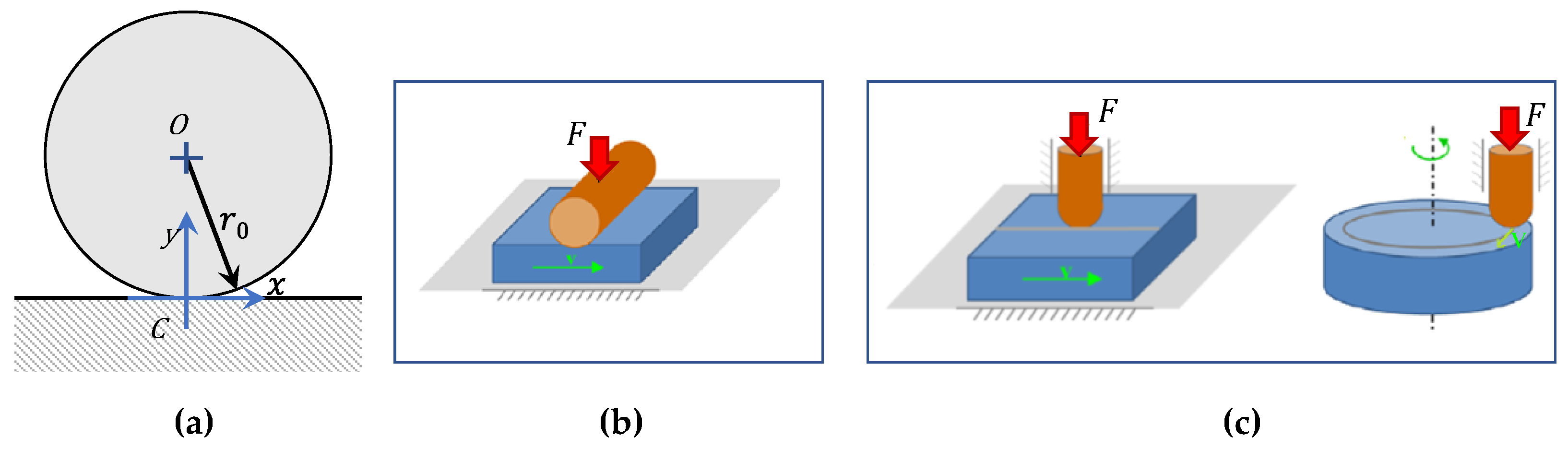
The procedure presented in [12] was focused on 2D problems and was specifically detailed for two pin-on-plate test cases, distinguished for the shape of the pin head: (a) cylindrical, for a line contact (LC) condition and (b) spherical, for point contact (PC) condition. In this study, we intended to further validate the procedure for these cases, which are particularly meaningful because they can be compared with experimental data.
With reference to Figure 1a, the surfaces in contact could be initially described by a straight line for the plate (y = 0), and a portion of the circumference defined by the following equation for the pin:
In the initial condition, the contact problem could be solved according to Hertzian formulas that employ the equivalent curvature radius and Young modulus which is generally defined as:
where subscripts 1–2 identify the two bodies (1 = pin, 2 = plate), E is the Young modulus and v is the Poisson ratio. For t = 0, in the unworn condition, we could replace . Furthermore, assuming that only the pin would be affected by wear, the curvature of the plate also remained null also during the whole wear process, so that:
According to Hertz, denoting by F the load per unit length for LC and the force for PC, the maximum contact pressure could be calculated as
Thus, the initial maximum contact pressures became:
and the contact half-widths in the unworn state were:
Still according to Hertz, both in LC and PC, the pressure was maximum at the center and null at the boundary of the contact region, following a semi-elliptical distribution:
where x is a radial coordinate in PC.
The combined action of pressure p and sliding velocity , produced wear on the pin’s surface, whose profile changed with time
where represents the wear depth term and null for t = 0. It should be noted that wear is considered to occur in the y direction, i.e., normal to the harder surface. The Archard wear law was frequently applied to estimate the rate of linear wear as:
where k is a dimensional wear factor. Equation (9) represents the general, local and instantaneous form of the Archard wear law. For translating couplings with constant sliding velocity during the whole process, such as those focused on the present study, we could write and the integration of Equation (9) provided the global form:
which describes a linearly increasing wear volume with time, or with the sliding distance d, replacing .
A modification of the pin profile due to wear produced a redistribution of the contact pressure evolving toward a more conformal case. This process could be described as an iterative modification of pressure and geometry. It was easily proved that, as the wear proceeded, the contact area widened. Thus, Equation (9) suggested another important observation: pressure at the border of the contact region could not be zero; otherwise, the contact area would not change. This meant that the Hertzian profile was not adequate to describe this phenomenon, and a modification was necessary. In our previous study [12], we proposed to replace the elliptic profile with a parabolic one according to the following equations:
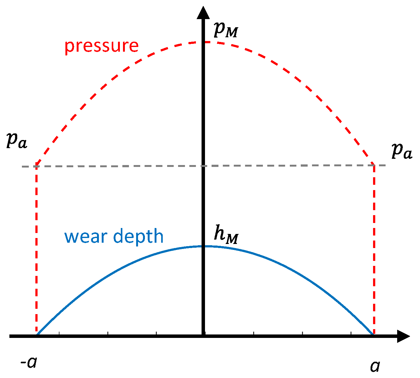
where pM is the maximum pressure, pa the pressure at the border of the contact area, a the contact half-width, as explained in Figure 2. During wear/time the three quantities pM pa and a varied continuously.
Similarly, the wear profile can be described by a parabolic trend:
as confirmed by Finite Element simulations, where is the maximum wear depth at the center of the contact area. Considering Equation (9), for a uniform velocity, pressure and wear trends can be connected through the following equations:
It must be noted that while cannot be derived from the Hertz theory, the maximum pressure is still obtainable from Equation (4), depending on the curvature radius in the nominal contact point C, , i.e.,
According to the fundamental geometrical properties of a curve, we first considered that the curvature is the inverse of the radius of curvature and can be calculated as:
.
Therefore, can be obtained by replacing Equation (12) with Equation (8) and applying the definition in (16).
So far, we had a problem with five unknowns () but only four equations, i.e., Equations (13)–(15) and (17). The fifth equation was the equilibrium condition that replaced Equation (6) to estimate , i.e.:
from which the following expressions could be obtained for the line and point contacts, respectively:
providing fundamental relationships between the maximum wear depth, the contact half-width and time.
The solution to this problem could be conveniently formulated through differential equations of the first order in the variable
and
for the line and point contacts, respectively.
The solution can be obtained numerically, e.g., using ode23 solver in Matlab® for t > 0 or in a discrete form implementing a simple cycle, and the whole procedure required only four simple lines in Matlab®, in addition to input data.
3. Test Cases
In our previous study [12], this procedure was validated with two test cases that we had already published in the literature, based on Finite Element simulations [7,13]. As explained in the introduction, in this work other papers have been considered to (a) further prove the validity of the procedure with data from other research groups, (b) solve some discrepancies observed in the first results, (c) include frictional contacts as possible application cases.
We selected study [16] for line contacts with the experimental data, [15] for FE results alongside frictional line contacts and [3,6] point contacts. The selection was based on studies with unilateral wear, with complete data for simulations and possibly including a comparison with experimental tests. Rather unexpectedly, not many papers satisfied the above requirements since, in most cases, data were incomplete.
3.1. Line Contact
In [16], several experimental tests were described on a cylindrical pin made of sintered polyimide in reciprocating sliding over a counter steel (high-alloy 40 CrMnNiMo846) plate. The main features of the tribotests considered in this study for the further validation of the procedure are summarized in Table 1 and Table 2.
Wear results were reported using different quantities, e.g., worn mass (mw), vertical displacement (dv) and modified diameter. We used the worn mass to estimate the wear coefficient, given the density of the worn material ( g/cm3); thus,
and, in the results, we compared the experimental dv to the predicted wear depths.
3.2. Frictional Line Contact
In a recent study [15], we investigated the effect of friction on conformal and non-conformal plane contacts. The negligible effect of friction on wear quantities was proved for a coefficient of friction up to 0.4. Here, we compared such FE data where friction was considered to the data we obtained with the present procedure (where the effect of friction was not included, vd. Section2). Furthermore, a refined FE model was used to investigate pressure distribution on the contact region to improve its description at the boundaries.
The main features of the simulated conditions are summarized in Table 3.
3.3. Point Contact
In the first test case for the point contact model, we selected the one described in [6], focusing on experimental tests and simulations of a brass pin sliding on a steel disc. All details of the point contact test case [6] are summarized in Table 4.
Main experimental wear results are also provided in the paper and reported in Table 5.
However, since we found some inconsistencies in the data, the worn volumes in Table 5 were 10 times those reported in [6]. This modification made the experimental values (wear depth and diameter of the worn area of Table 6, in addition to worn volume) consistent with formulas in the ASTM G99:
Consequently, the wear factors also differed from the original values.
The second test case was the study from Hegadekatte et al. [3], where numerical and finite element models were presented and compared with experimental data. In particular, the authors described a global incremental wear model (GIWM) that provided a discretized solution for wear evolution for an application focused on the system analysis of a micro-turbine and a micro-planetary gear train. The maximum wear depth was estimated according to a cyclic routine. Here, it is related, through the Archard model, to the average pressure over the contact area, i.e., instead of Equation (13), the following assumption was introduced:
where:
This model was used to simulate a pin-on-disc wear test (data in Table 6) for pin and disc samples in silicon nitrite. The study also aimed to evaluate a modified wear factor where friction appeared explicitly.
In [3], experimental results consist of the trend of hM over the test, which was continuously measured capacitively within a resolution of ±1 μm. Since the wear of the disc was below 200 nm, we could consider it negligible with respect to the pins so we could use of our model.
4. Results and Discussion
4.1. Line Contact
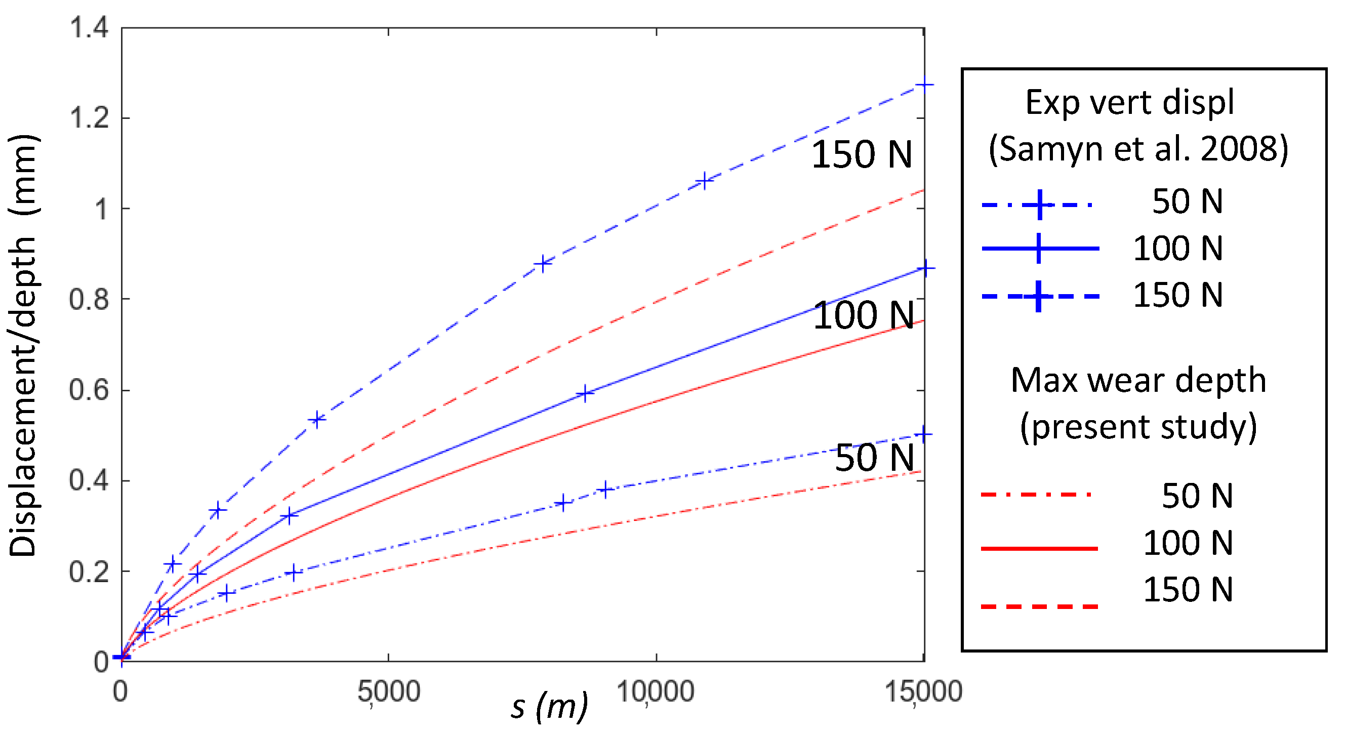
The application of the proposed procedure to the first test case on line contacts provided results that were in rather good agreement with those in [16], as shown in Figure 3, where the experimental vertical displacements measured during the tests for different load levels are compared with the maximum predicted wear depths. We chose to compare these quantities since they were the nearest ones on the experimental and numerical sides. Their difference was expected, as discussed in [16], due to creep, thermal expansion and other viscoelastic effects. For the 50 N case, an ‘offline’ correction of the vertical displacement at the end of the test reduced it from 0.51 mm to 0.43 mm, which was much similar to the predicted value of 0.42 mm. A similar correction could also be expected to reduce differences for other loads.
4.2. Frictional Line Contact
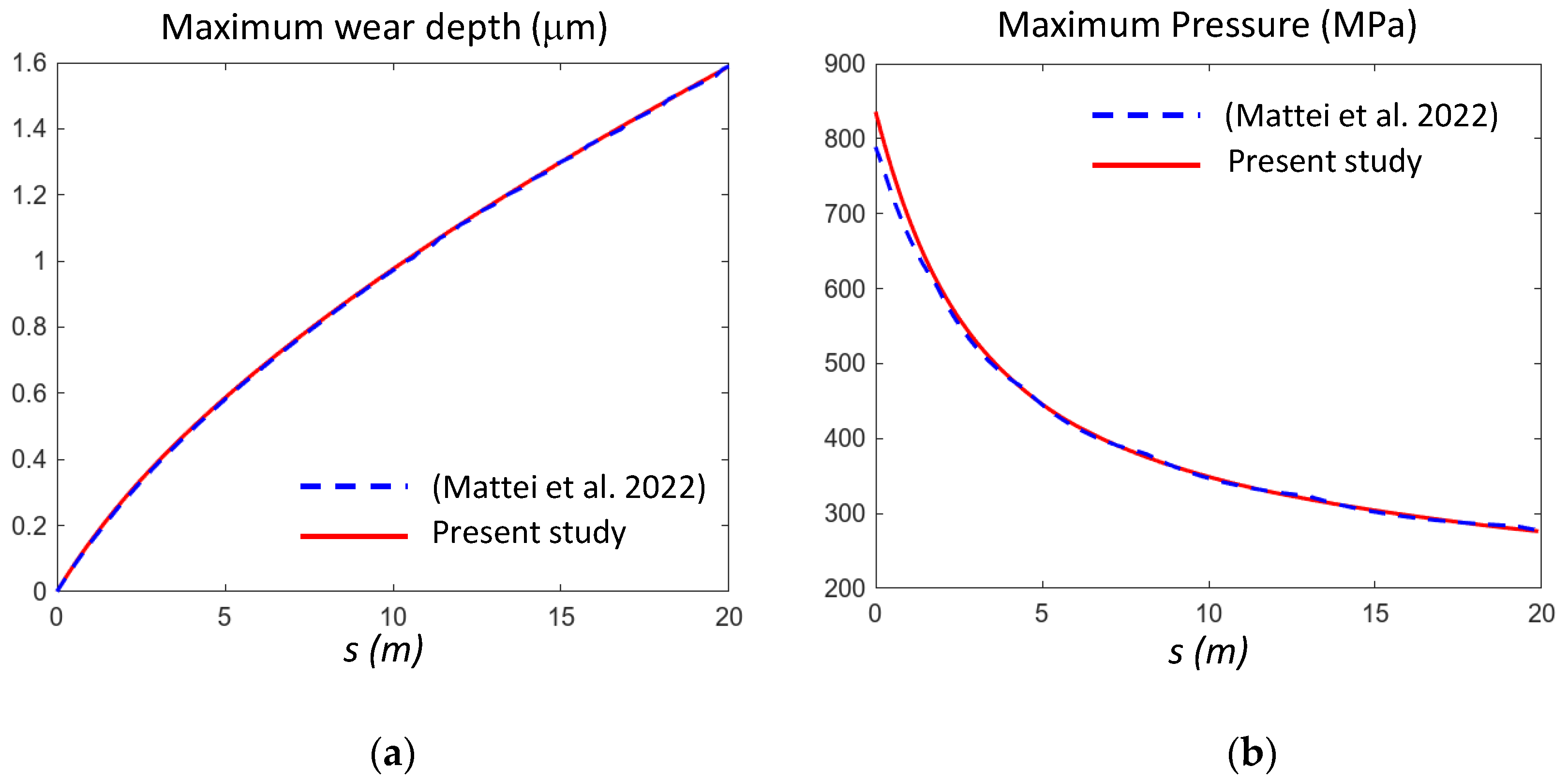
Figure 4 contains the main results of the analytical approach compared to FE results from [15]. It can be observed that the maximum wear depth and maximum pressure were perfectly overlapped, which confirmed the reliability of the proposed procedure.
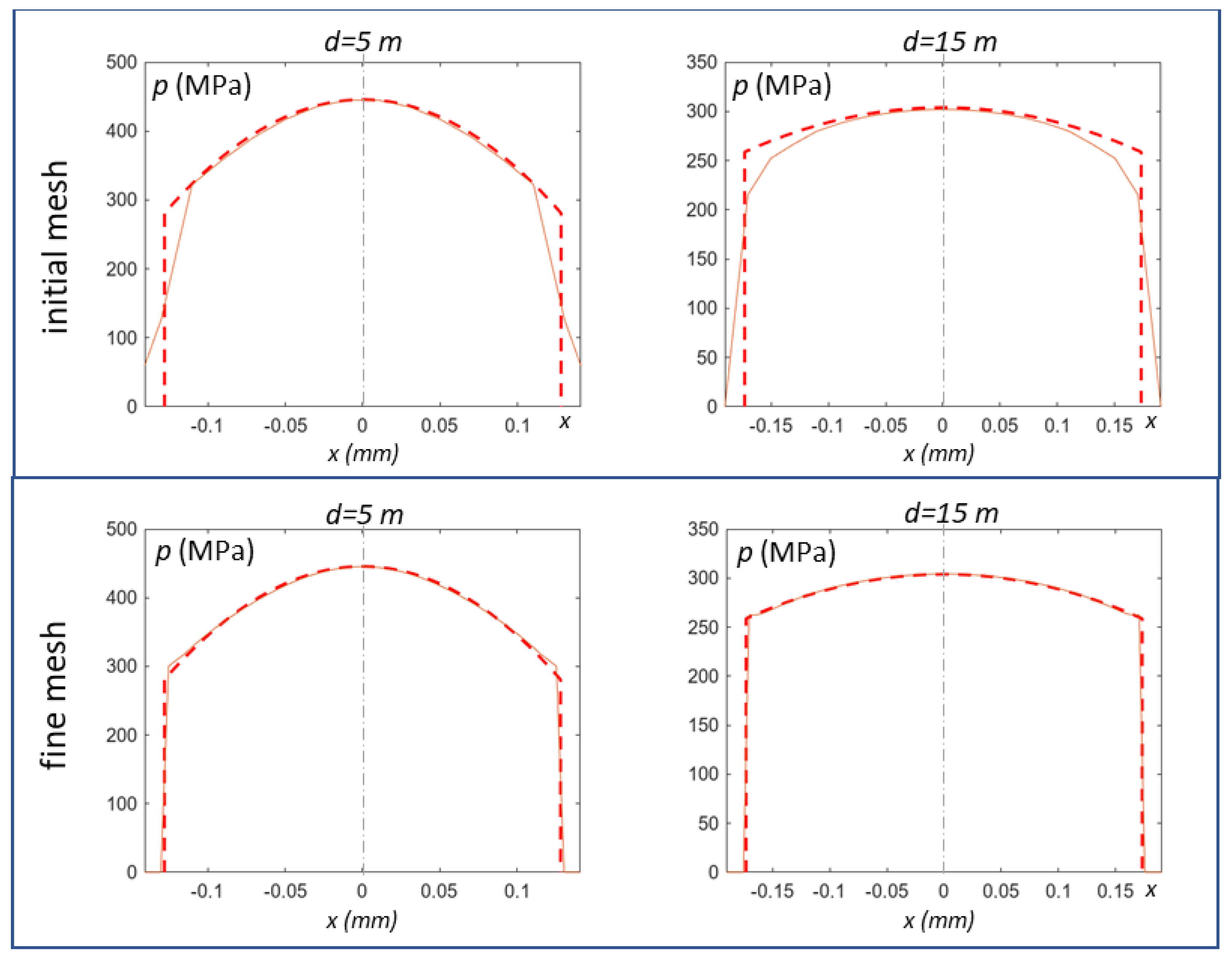
In our previous study [12], major discrepancies between the analytical and the FE solutions were observed in pressure distribution at the boundaries of the contact region. The mesh, whose results are depicted in Figure 4, provided pressure profiles over the contact region reported in the first row of Figure 5 for two selected traveled distances (d = 5–15 m). They confirmed that the rapid gradient at the boundaries caused the main difference between the two trends, while the maximum pressure was correctly estimated.
However, when refining the FE mesh at the boundaries, the curves appeared perfectly overlapped, as described in the second row of Figure 5, indicating that the hypothesis on pressure distribution in Equation (11) was correct and flexible enough to depict changes from parabolic to uniform pressure profiles.
4.3. Point Contact
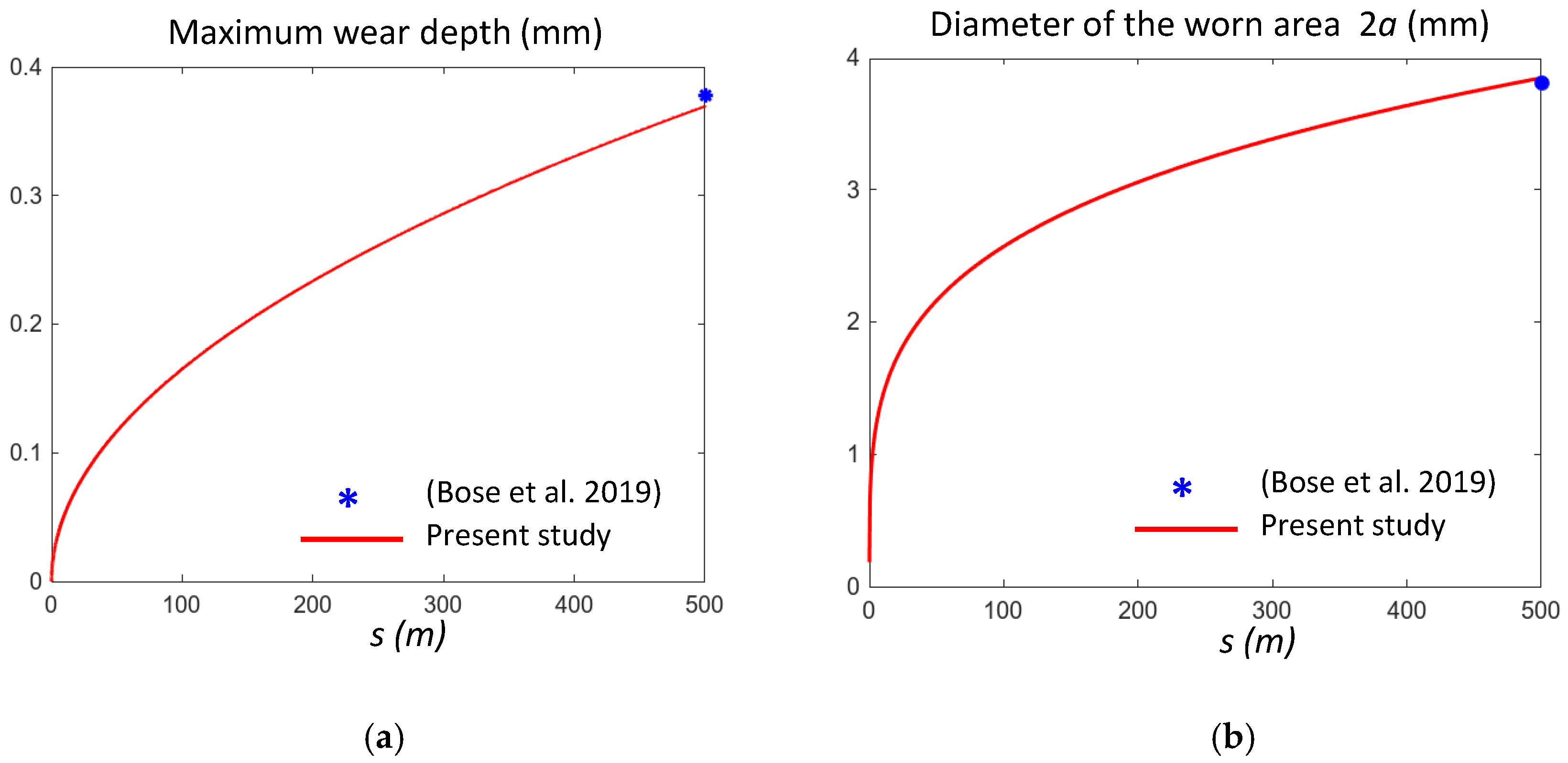
The point contact procedure was compared to the case described in Bose [6], with three force levels. Firstly, the estimated maximum wear depth and diameter of the contact area were compared with those obtained experimentally at the end of tests, as shown in Figure 6 for F = 10 N (Test 1) and in Table 7 for all three cases. A very good agreement could be observed, with percentage errors lower than 2.5%.
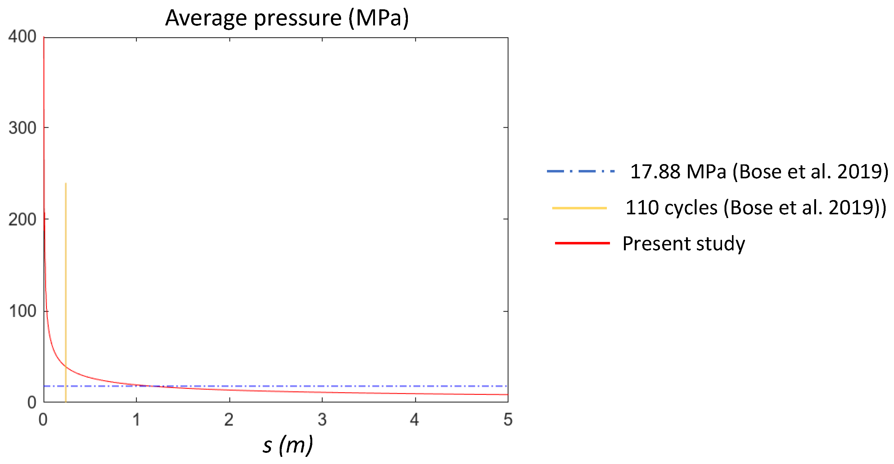
Moreover, in [6], the evolution of the average pressure during wear was investigated and related to a threshold value in order to reduce the number of Finite Element analyses performed in Abaqus and limit the computational cost. Increments in the sliding distance of 2 mm were considered for each cycle. Since the average pressure rapidly decreased with wear, a threshold cycle value distinguishing a variable and a constant pressure field could be introduced. In [6], it was reported that such a cycle for F = 10 N is the 110th, corresponding to an average pressure of 17.88 MPa. Figure 7 shows the average pressure trend obtained with the proposed procedure, with a threshold value of 17.88 MPa, and cycle 110. It can be observed that the average threshold value was reached only at about 1 m (not at 0.22 m corresponding 110th cycle).
This indicates that despite the Abaqus fine model and the high number of cycles, the correct trend was not achieved. This observation stresses the important role and simplicity of the proposed approach with respect to more complex and time-consuming Finite Element simulations.
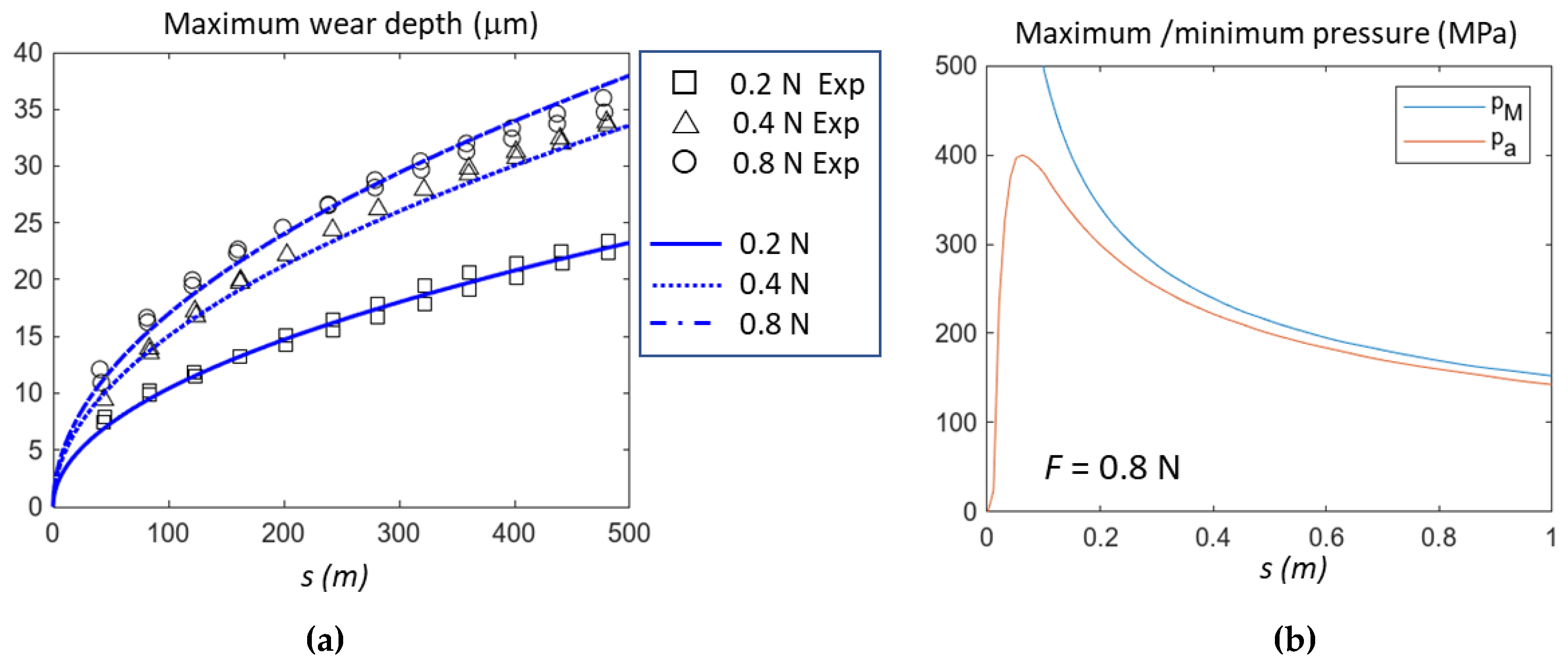
As far as the study in [3] is concerned, the maximum wear depth we obtained is depicted in Figure 8, comparing the experimental and analytical results. For tests under a load equal to 0.2 N and 0.4 N, the k value is the one reported in Table 4, while for F = 0.8 N, this was reduced to 13.5·10−9 mm2 N to fit the experimental data. It must be observed that it was not clear whether the experimental measure actually provided the maximum depth or a kind of average value over the contact area. According to the parabolic assumption, the ratio between the average and maximum wear depth was about 0.78; taking this into account, we should rescale all k values.
It must be noted that our model provides very similar results to those derived by Hegadekatte et al. with the GIWM, despite the fact that we had more detailed (not averaged) wear and pressure distributions than GIWM. The reason for this similarity can be found in Figure 8 (right), where it is clear that the maximum and the minimum pressures become similar very soon, after about 0.2 m, i.e., only for the first 0.04% of the wear test.
5. Conclusions
The present study aimed to further validate the simple and efficient analytical approach proposed for wear predictions in both line and contact points, as previously presented by the authors. Attention was given to the validity of the approach both to simulate frictional contacts and the pressure profile at the contact boundaries, where it changed drastically.
To this purpose, both experimental and numerical wear studies were selected in the literature when fully reproducible and were simulated using the novel approach. Our wear predictions in terms of volumetric and maximum linear wear depth and worn area, as well as contact pressure, were almost overlapped in the literature results with errors lower than 2.5%, thus proving the reliability of the assumptions and the procedure.
The strong point of the proposed analytical method was, firstly, the simplicity of its implementation: the evolution of pressure and wear could be easily implemented in a few lines of codes by solving a first-order differential equation; secondly, it allowed long term wear predictions in a few seconds, overcoming one of the main limits of the counterpart Finite Element simulations. Thus, it is a reliable tool for researchers and engineers who are attempting to obtain rapid and reliable wear indications for many different practical problems.
Author Contributions
Methodology, F.D.P. and L.M.; Formal analysis, F.D.P. and L.M.; Data curation, L.M.; Writing—original draft, F.D.P.; Writing—review & editing, F.D.P. and L.M. All authors have read and agreed to the published version of the manuscript.
Funding
This research received no external funding.
Data Availability Statement
Research data are unavailable.
Conflicts of Interest
The authors declare no conflict of interest.
References
- Grabovic, E.; Artoni, A.; Gabiccini, M.; Guiggiani, M.; Mattei, L.; Di Puccio, F.; Ciulli, E. Friction-Induced Efficiency Losses and Wear Evolution in Hypoid Gears. Machines 2022, 10, 748. [Google Scholar] [CrossRef]
- Mattei, L.; Di Puccio, F.; Joyce, T.J.; Ciulli, E. Effect of size and dimensional tolerance of reverse total shoulder arthroplasty on wear: An in-silico study. J. Mech. Behav. Biomed. Mater. 2016, 61, 455–463. [Google Scholar] [CrossRef] [PubMed]
- Hegadekatte, V.; Kurzenhäuser, S.; Huber, N.; Kraft, O. A predictive modeling scheme for wear in tribometers. Tribol. Int. 2008, 41, 1020–1031. [Google Scholar] [CrossRef]
- Öqvist, M. Numerical simulations of mild wear using updated geometry with different step size approaches. Wear 2001, 249, 6–11. [Google Scholar] [CrossRef]
- Bortoleto, E.; Rovani, A.; Seriacopi, V.; Profito, F.; Zachariadis, D.; Machado, I.; Sinatora, A.; Souza, R. Experimental and numerical analysis of dry contact in the pin on disc test. Wear 2013, 301, 19–26. [Google Scholar] [CrossRef]
- Bose, K.; Penchaliah, R. 3-D FEM Wear Prediction of Brass Sliding against Bearing Steel Using Constant Contact Pressure Approximation Technique. Tribol. Online 2019, 14, 194–207. [Google Scholar] [CrossRef]
- Curreli, C.; Di Puccio, F.; Mattei, L. Application of the finite element submodeling technique in a single point contact and wear problem. Int. J. Numer. Methods Eng. 2018, 116, 708–722. [Google Scholar] [CrossRef]
- Di Puccio, F.; Mattei, L. In-silico Analytical Wear Predictions: Application to Joint Prostheses. In Wear in Advanced Engineering Applications and Materials; World Scientific: Lodon, UK, 2022; pp. 123–148. [Google Scholar] [CrossRef]
- Argatov, I.; Chai, Y. A self-similar model for fretting wear contact with the third body in gross slip. Wear 2021, 466–467, 203562. [Google Scholar] [CrossRef]
- Mattei, L.; Di Puccio, F.; Joyce, T.; Ciulli, E. Numerical and experimental investigations for the evaluation of the wear coefficient of reverse total shoulder prostheses. J. Mech. Behav. Biomed. Mater. 2016, 55, 53–66. [Google Scholar] [CrossRef] [PubMed]
- Rodríguez-Tembleque, L.; Abascal, R.; Aliabadi, M. A boundary elements formulation for 3D fretting-wear problems. Eng. Anal. Bound. Elem. 2011, 35, 935–943. [Google Scholar] [CrossRef]
- Di Puccio, F.; Mattei, L. Simple analytical description of contact pressure and wear evolution in non-conformal contacts. Tribol. Int. 2023, 178, 108084. [Google Scholar] [CrossRef]
- Mattei, L.; Di Puccio, F. Influence of the wear partition factor on wear evolution modelling of sliding surfaces. Int. J. Mech. Sci. 2015, 99, 72–88. [Google Scholar] [CrossRef]
- Mattei, L. Effect of Friction on Finite Element Contact and Wear Predictions of Metal-on-Plastic Hip Replacements. Biotribology 2023, 35–36, 100230. [Google Scholar] [CrossRef]
- Mattei, L.; Di Puccio, F. Frictionless vs. frictional contact in numerical wear predictions of conformal and non-conformal sliding couplings (Accepted for publication). Tribol. Lett. 2022, 70, 115. [Google Scholar] [CrossRef]
- Samyn, P.; Quintelier, J.; Schoukens, G. On the Repeatability of Friction and Wear Tests for Polyimides in a Hertzian Line Contact. Exp. Mech. 2008, 48, 233–246. [Google Scholar] [CrossRef]
Figure 1.
(a) Definition of the geometry in the x-y plane. Schemes of the test cases: (b) Line contact: pin-on-plate test, (c) Point contact: pin-on-plate/disc test.
Figure 1.
(a) Definition of the geometry in the x-y plane. Schemes of the test cases: (b) Line contact: pin-on-plate test, (c) Point contact: pin-on-plate/disc test.

Figure 2.
Wear depth and pressure profiles.

Figure 3.
Comparison of the predicted maximum wear depth (in red) and the experimental vertical displacement (in blue) from Samyin et al. 2008 [16] at three load levels (50, 100, 150 N).
Figure 3.
Comparison of the predicted maximum wear depth (in red) and the experimental vertical displacement (in blue) from Samyin et al. 2008 [16] at three load levels (50, 100, 150 N).

Figure 4.
Comparison of the maximum wear depth (a) and maximum pressure (b) obtained from the proposed approach and from FE simulations (Mattei et al. 2022) [15].
Figure 4.
Comparison of the maximum wear depth (a) and maximum pressure (b) obtained from the proposed approach and from FE simulations (Mattei et al. 2022) [15].

Figure 5.
Comparison of the pressure profiles obtained from the proposed procedure and from FE simulations [15] for two travelled distances d = 5 m (left) and d = 15 m (right). First row: FE model with a rather fine mesh; second row: FE model with mesh refined at the borders. (Legend as in Figure 4: red solid line = present study; dashed blue line = FE solution from [15]).

Figure 6.
Predicted trends of the maximum wear depth (a) and diameter (b) of the worn area (i.e., 2 a) compared to the experimental values (the blue *) at the end of the test 1 for F = 10 N from (Bose et al., 2019) [6].
Figure 6.
Predicted trends of the maximum wear depth (a) and diameter (b) of the worn area (i.e., 2 a) compared to the experimental values (the blue *) at the end of the test 1 for F = 10 N from (Bose et al., 2019) [6].

Figure 7.
Average pressure obtained with the proposed procedure and identification of a threshold value (17.88 MPa); that in (Bose et al. 2019) [6] is found at cycle 110, (F = 10 N).
Figure 7.
Average pressure obtained with the proposed procedure and identification of a threshold value (17.88 MPa); that in (Bose et al. 2019) [6] is found at cycle 110, (F = 10 N).

Figure 8.
(a): Comparison of maximum wear depth: experimental data vs. analytical model, Average pressure obtained with the proposed procedure and identification of a threshold value (17.88 MPa); that in [6] is found at cycle 110, (F = 10 N). (b): Maximum (pM) and minimum (pa) pressure in the first part of the test for F = 0.8 N.


Table 1.
Main data for the three experimental test cases [16].
Table 1.
Main data for the three experimental test cases [16].
| Ref. | r0 (mm) | L (mm) | E1 (MPa) | ν1 | E2 (GPa) | ν2 | FN (N) | k (mm2/N) | vs (m/s) | d (m) |
|---|---|---|---|---|---|---|---|---|---|---|
| [16] | 2.5 | 15 | 2480 | 0.4 | 200 | 0.3 | 50, 100, 150 | 10−8 | 0.3 | 15,000 |
Table 2.
Wear results and wear coefficient for three tested conditions [16].
Table 2.
Wear results and wear coefficient for three tested conditions [16].
| Tests | FN (N) | mw (g) | k (mm2/N) |
|---|---|---|---|
| Test 1 | 50 | 0.0164 | 1.63·10−8 |
| Test 2 | 100 | 0.0392 | 1.95·10−8 |
| Test 3 | 150 | 0.0367 | 2.11·10−8 |
Table 3.
Main data of the test case in [15].
Table 3.
Main data of the test case in [15].
| Ref. | r0 (mm) | E (GPa) | ν | F (N/mm) | k (mm2/N) | vs (m/s) | d (m) |
|---|---|---|---|---|---|---|---|
| [15] | 10 | 200 | 0.3 | 100 | 10−8 | 0.01 | 20 |
Table 4.
Main data of the test case in [6].
Table 4.
Main data of the test case in [6].
| Ref. | r0 (mm) | Ep (GPa) | νp | Ed (GPa) | νd | F (N) | vs (m/s) | d (m) |
|---|---|---|---|---|---|---|---|---|
| [6] | 5 | 100 | 0.33 | 200 | 0.3 | 10, 20, 30 | 0.4 | 500 |
Table 5.
Wear volume and wear coefficient for three tested conditions [6].
Table 5.
Wear volume and wear coefficient for three tested conditions [6].
| Tests | F (N) | Vw (mm3) | k (mm2/N) |
|---|---|---|---|
| Test 1 | 10 | 2.144 | 42.288·10−8 |
| Test 2 | 20 | 3.67 | 36.7·10−8 |
| Test 3 | 30 | 5.501 | 36.66·10−8 |
Table 6.
Main data of the test case in [3].
Table 6.
Main data of the test case in [3].
| Ref. | r0 (mm) | Ep = Ed (GPa) | F (N) | vs (m/s) | d (m) | k (mm2 N) | |
|---|---|---|---|---|---|---|---|
| [3] | 0.794 | 304 | 0.24 | 0.2, 0.4, 0.8 | 0.4 | 500 | 13.5·10−9 |
Table 7.
Comparison of experimental and estimated wear depths and contact area diameters [6].
Table 7.
Comparison of experimental and estimated wear depths and contact area diameters [6].
| Test | Experimental Wear Depth (mm) | Estimated Wear Depth (mm) | Error (%) | Experimental Worn Area Diameter (mm) | Estimated Worn Area Diameter (mm) | Error (%) |
|---|---|---|---|---|---|---|
| Test 1 | 0.378 | 0.369 | 2.4 | 3.805 | 3.84 | −0.92 |
| Test 2 | 0.493 | 0.4834 | 1.9 | 4.329 | 4.397 | −1.57 |
| Test 3 | 0.602 | 0.5918 | 1.7 | 4.758 | 4.8654 | −2.25 |
Disclaimer/Publisher’s Note: The statements, opinions and data contained in all publications are solely those of the individual author(s) and contributor(s) and not of MDPI and/or the editor(s). MDPI and/or the editor(s) disclaim responsibility for any injury to people or property resulting from any ideas, methods, instructions or products referred to in the content. |
© 2023 by the authors. Licensee MDPI, Basel, Switzerland. This article is an open access article distributed under the terms and conditions of the Creative Commons Attribution (CC BY) license (https://creativecommons.org/licenses/by/4.0/).
Share and Cite
MDPI and ACS Style
Di Puccio, F.; Mattei, L. Further Validation of a Simple Mathematical Description of Wear and Contact Pressure Evolution in Sliding Contacts. Lubricants 2023, 11, 230. https://doi.org/10.3390/lubricants11050230
AMA Style
Di Puccio F, Mattei L. Further Validation of a Simple Mathematical Description of Wear and Contact Pressure Evolution in Sliding Contacts. Lubricants. 2023; 11(5):230. https://doi.org/10.3390/lubricants11050230
Chicago/Turabian StyleDi Puccio, Francesca, and Lorenza Mattei. 2023. "Further Validation of a Simple Mathematical Description of Wear and Contact Pressure Evolution in Sliding Contacts" Lubricants 11, no. 5: 230. https://doi.org/10.3390/lubricants11050230
Note that from the first issue of 2016, this journal uses article numbers instead of page numbers. See further details here.