A Saturation-Based Method for Primary Resonance Control of Flexible Manipulator

Abstract

When primary resonance occurs, even a small external disturbance can abruptly excite large amplitude vibration and deteriorate the working performance of a flexible manipulator. Most active control methods are effective for non-resonant vibration but not for primary resonance. In view of this, this paper puts forward a new nonlinear saturation-based control method to suppress the primary resonance of a flexible manipulator considering complicated rigid-flexible coupling and modal coupling. A vibration absorber with variable stiffness/damping is designed to establish an energy exchange channel for saturation. A novel idea of modal coupling enhancement is suggested to improve saturation performance by strengthening the coupling relationship between the mode of the vibration absorber and the controlled mode of the flexible manipulator. Through stability analysis on the primary resonance response of the flexible manipulator with the vibration absorber, the saturation mechanism is successfully established and the effectiveness of the saturation control algorithm is validated. On this basis, several important indexes are extracted and employed to optimize saturation control. Finally, a series of virtual prototyping simulations and experiments are conducted to verify the feasibility of the suggested saturation-based control method. This research will contribute to the primary resonance suppression of a flexible manipulator under a complex external excitation environment.

1. Introduction

With the rapid development of modern space technology, the flexible manipulator plays an important role in space maintenance, machining, and assembly due to its advantages of low energy consumption and large load–weight ratio [1,2]. However, flexible manipulators are prone to vibration due to the existence of structural flexibility. Therefore, the vibration control problem has attracted extensive attention [3,4,5].

When performing some reciprocating work, such as spot welding, spray painting, carrying, and assembly, the flexible manipulator may be subjected to periodic external excitation. If the excitation frequency is close to the natural frequency of the flexible manipulator, primary resonance will occur [6]. In this case, even a small external excitation can abruptly excite large amplitude vibration and deteriorate working performance. Up to now, various nonlinear characteristics and stability problems of the primary resonance have been researched. Silva and Daqaq [7] analyzed the nonlinear vibration response of a sender cantilever beam with constant thickness and linearly varying width when subjected to a primary resonance excitation. Mokhtari and Jalili et al. [8] modeled a milling tool as a 3D spinning cantilever Timoshenko beam and investigated the primary resonance and the bifurcation behavior during micro-milling operations. Gao and Hou et al. [9] discussed the effect of the linear stiffness and the nonlinear stiffness of the inter-shaft bearing on the primary resonance and found the jump phenomenon and the resonance hysteresis phenomenon of a dual-rotor system. Kumar and Pratiher [10] studied the primary resonance behavior of the two-link flexible manipulator with a generic payload and constraint force through numerical simulations. They found the jump phenomenon and the existence of multi-valued solutions at pitchfork and saddle-node bifurcation points. Ding and Huang et al. [11] investigated the primary resonance of traveling viscoelastic beam under 3:1 internal resonance. Lajimi and Heppler et al. [12] used the method of multiple scales and the shooting method to study primary resonance of a beam-rigid body microgyroscope. Li and Yao et al. [13] studied the effects of control gains on primary resonance properties of the beam. Bab and Khadem et al. [14] investigated the primary resonances of a coupled flexible rotor with rigid disk and flexible/rigid blades. Zhang and Chen et al. [15] analyzed the primary resonance of coupled cantilevers subjected to magnetic interaction based on the distributed parameter model. Li and Zhou et al. [16] studied the primary resonance with internal resonance of a symmetric rectangular honeycomb sandwich panel with simply supported boundaries along all four edges subjected to transverse excitations. Yektanezhad and Hosseini et al. [17] investigated primary resonance of a flexible rotor levitated by active magnetic bearings (AMBs). Gu and Zhang et al. [18] investigated the primary resonance of the functionally graded graphene platelet (FGGP)-reinforced rotating pre-twisted composite blade under combined external and multiple parametric excitations with three different distribution patterns. Arena and Lacarbonara [19] implemented bifurcation analysis to investigate the primary resonances induced by the harmonic axial excitation.

In order to deal with the vibration problems, many active control methods have been put forward. However, most of them are effective for non-resonant vibration but not for primary resonance. In recent years, the saturation phenomenon has attracted the attention of many researchers. This phenomenon usually occurs in a quadratic nonlinear system under the harmonic excitation if the ratio of two modal frequencies is 1:2 and the internal resonance has been established between these two modes. When the excitation frequency is close to the high-order modal frequency of the system, the higher-order modal response will increase. When the saturation occurs, the higher modal response will no longer increase after it reaches a critical value, and the rest of vibration energy is transferred to the lower-order mode. Nayfeh and Mook [20] first discovered the saturation phenomenon by analyzing the coupling between the roll and pitch motion of ships. Haddow and Barr et al. [21] verified the saturation phenomenon by the modal interaction experiment of an L-shaped beam and suggested a saturation-based vibration absorber for controlling the primary resonance of a flexible structure. Subsequently, Oueini and Nayfeh et al. [22] proposed an active saturation-based method for controlling the primary resonance of a rigid and a flexible beam, respectively, and designed an analog circuit to verify the feasibility of the suggested method. Pai and Wen et al. [23] used PZT (lead zirconate titanate) patches as a controller and sensor to study the nonlinear saturation control of a cantilever beam. Saguranrum and Kunz et al. [24] numerically simulated the saturation control response and the full mode coupling of the cantilever beam with a piezoelectric actuator. Shoeybi and Ghorashi [25] conducted a theoretical investigation of nonlinear vibrations of a 2-DOF system when subjected to saturation. Li et al. [26] used the method of multiple scales to obtain an approximate analytical solution and presented a control strategy based on nonlinear saturation to suppress the free vibration of a self-excited plant. Zhao and Xu [27] applied the delayed feedback control and saturation control to suppress or stabilize the vibration of the primary system in a 2-DOF dynamical system with parametrically excited pendulum. Eftekhari and Ziaei-Rad [28] investigated the performance of an oscillator consisting of mass and spring at the tip of a symmetrical cantilever composite beam under chordwise base excitation and detected saturation phenomenon in the force modulation response at the one-to-one internal resonance. Febbo and Machado [29] studied nonlinear dynamic vibration absorbers with a saturation. Chen and Zhang [30] investigated forced vibration for two elastically connected cantilevers under harmonic base excitation, and the frequency amplitude response curves revealed saturation phenomena. Zhang and Liu et al. [31] analyzed the saturation and jump phenomena of a rotating pre-twisted laminated composite blade subjected to a subsonic airflow excitation in the case of 1:2 internal resonance. Rocha and Tusset et al. [32] used the piezoelectric material to harvest the energy of a portal frame structure and found that the energy transfer efficiency can be enhanced by coupling the PZT to the column in saturation phenomena. Bauomy and Taha [33] studied the nonlinear vibrating behaviors of a nonlinear cantilever beam system (primary system) using a nonlinear saturation absorber (the secondary system).

Although saturation-based research has been conducted, it still faces big challenges when dealing with the primary resonance of a flexible manipulator. First, all the above studies are focused on a flexible structure without rigid motion. For a flexible multi-body mechanism undergoing a large overall motion, however, its dynamic model is completely different from that of a flexible structure due to complex rigid–flexible motion coupling and force transfer. To the authors’ knowledge, whether the saturation can be established and utilized to suppress the primary resonance of a flexible mechanism has not been researched. Second, most studies simplified the controlled main system as a linear vibration system for the convenience of analysis. However, a real system is usually a nonlinear system. Excessive neglect of nonlinear elements may lead to a mismatch with reality. Third, the saturation depends on the coupling between the controlled main system and the vibration absorber. However, this coupling relationship is artificially designated in most studies for the convenience of analysis and is not derived from a rigorous kinematic and dynamic relationship. Finally, most studies are based on numerical simulations of their own theoretical models and have not been verified by third-party software or experiments.

In view of this, this paper aims to put forward a new nonlinear saturation-based control method to suppress the primary resonance of the flexible manipulator undergoing a large overall motion. The rest of the paper is organized as follows. In Section 2, a controlled flexible manipulator is described. In Section 3, a new primary resonance control scheme is designed and a saturation-based control model of the vibration absorber is put forward. The dynamic equations of the flexible manipulator with the saturation-based vibration absorber are derived in Section 4. Because the saturation depends on the internal resonance, Section 5 investigates the establishment of the internal resonance. Section 6 reveals the saturation principle. Section 7 presents the method of absorber configuration to optimize saturation control. On this basis, a series of virtual prototyping simulations and experiments are conducted to verify the feasibility of the suggested saturation-based control method in Section 8 and Section 9. Section 10 explains the inaccurate correspondence of theory, prototype simulation, and experiment results. Finally, Section 11 summarizes the conclusions of this study.

2. Description of Flexible Manipulator

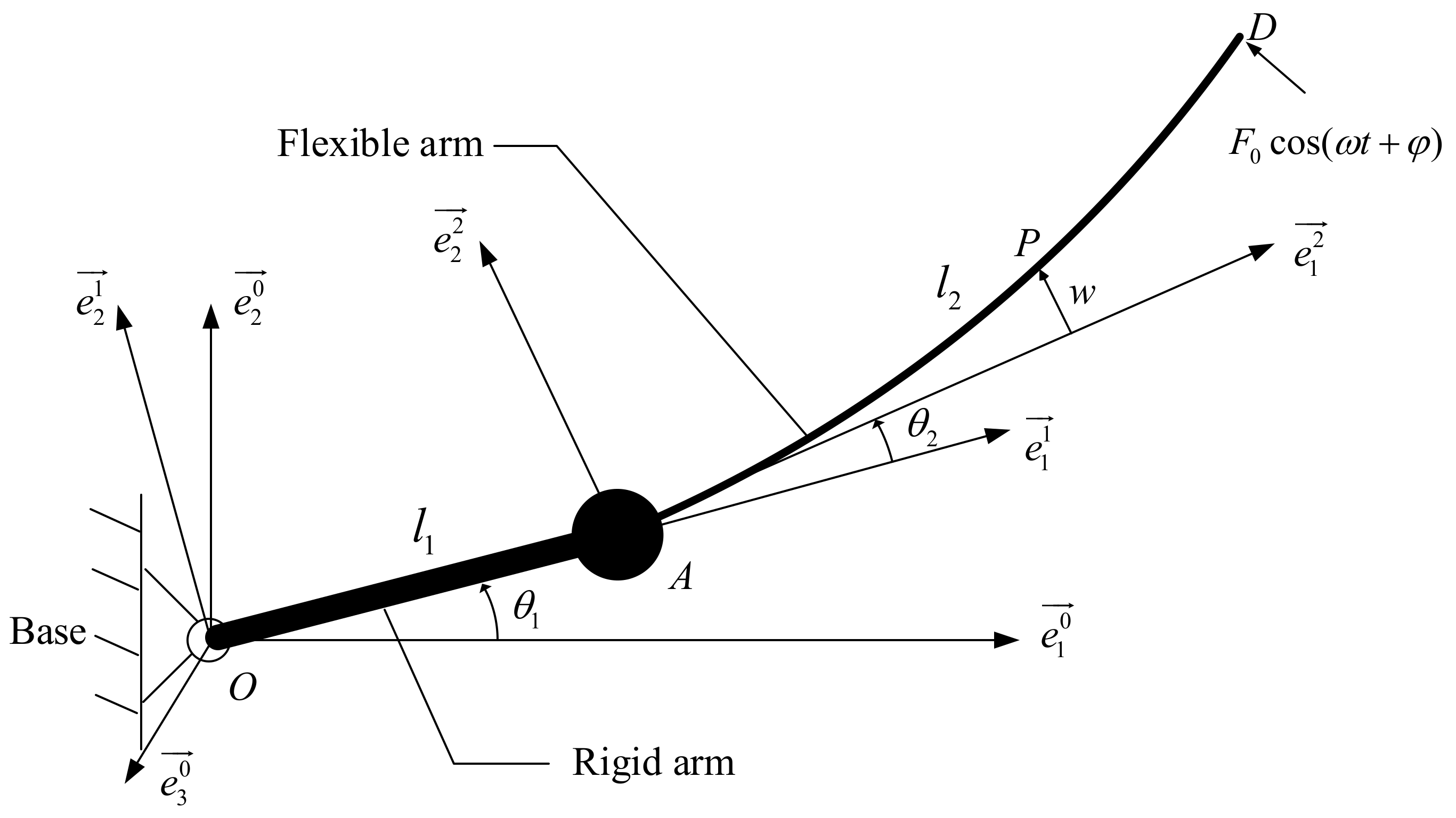
As shown in Figure 1, the flexible manipulator consists of a base, a rigid arm, and a flexible arm. The expression $O\overrightarrow{e_1^0}\overrightarrow{e_2^0}$ is the inertial coordinate system fixed on the base; $O\overrightarrow{e_1^1}\overrightarrow{e_2^1}$ and $A\overrightarrow{e_1^2}\overrightarrow{e_2^2}$ are the moving coordinate systems attached to the rigid and flexible arms, respectively. The rigid arm $OA$ is hinged to the driving joint $O$, whose angular displacement is denoted by ${\theta }_1(t)$, where $t$ is time. The flexible arm $AD$ is hinged to the driving joint $A$ at the end of the rigid arm, whose angular displacement is denoted by ${\theta }_2(t)$.

Due to the large span-to-height ratio, the flexible arm is regarded as a uniform Euler–Bernoulli beam. Only the transverse deformation of the flexible arm in $A\overrightarrow{e_1^2}\overrightarrow{e_2^2}$ is considered, which is denoted by $w\left(x,t\right)$, where x denotes the length measured along $A\overrightarrow{e_1^2}$. Using the assumed mode method [3], the deformation $w\left(x,t\right)$ is discretized as

$$w\left(x,t\right)={\displaystyle \mathbf{\sum }_{i=1}^n{\varphi }_i\left(x\right)q_i}\left(t\right),$$

(1)

where $n$ is the number of the flexural degrees of freedom, ${\varphi }_i\left(x\right)$ is the ith order model shape, and $q_i\left(t\right)$ is the ith mode coordinate.

Because the fundamental mode usually plays a major role in the dynamic responses of the flexible arm, only the fundamental mode is considered. Therefore, Equation (1) is rewritten as

$$w\left(x,t\right)\approx {\varphi }_1\left(x\right)q_1\left(t\right).$$

(2)

When the flexible manipulator is subjected to the external excitation $F=F_0\cos \left(\omega t+\phi \right)$ at the same frequency as its natural frequency, the primary resonance will occur. It may excite large amplitude in a short time and thus deteriorate the working performance and lead to system damage. Therefore, it is necessary to suppress the primary resonance. In view of this, a saturation-based control method is put forward in this paper to suppress the primary resonance of the flexible manipulator.

3. Control Model of Saturation-Based Vibration Absorber

Among various nonlinear interactions, saturation is a special energy exchange mechanism of a multiple degrees-of-freedom nonlinear system. Its generation depends on the establishment of the 1:2 internal resonance. When the saturation phenomenon occurs in a nonlinear system excited at a frequency near its high-order modal frequency, the primary resonance response of the high-order mode will be restricted to a small ceiling, and the rest of the vibration energy will be transferred to the low-order mode with the help of an energy exchange channel provided by the internal resonance.

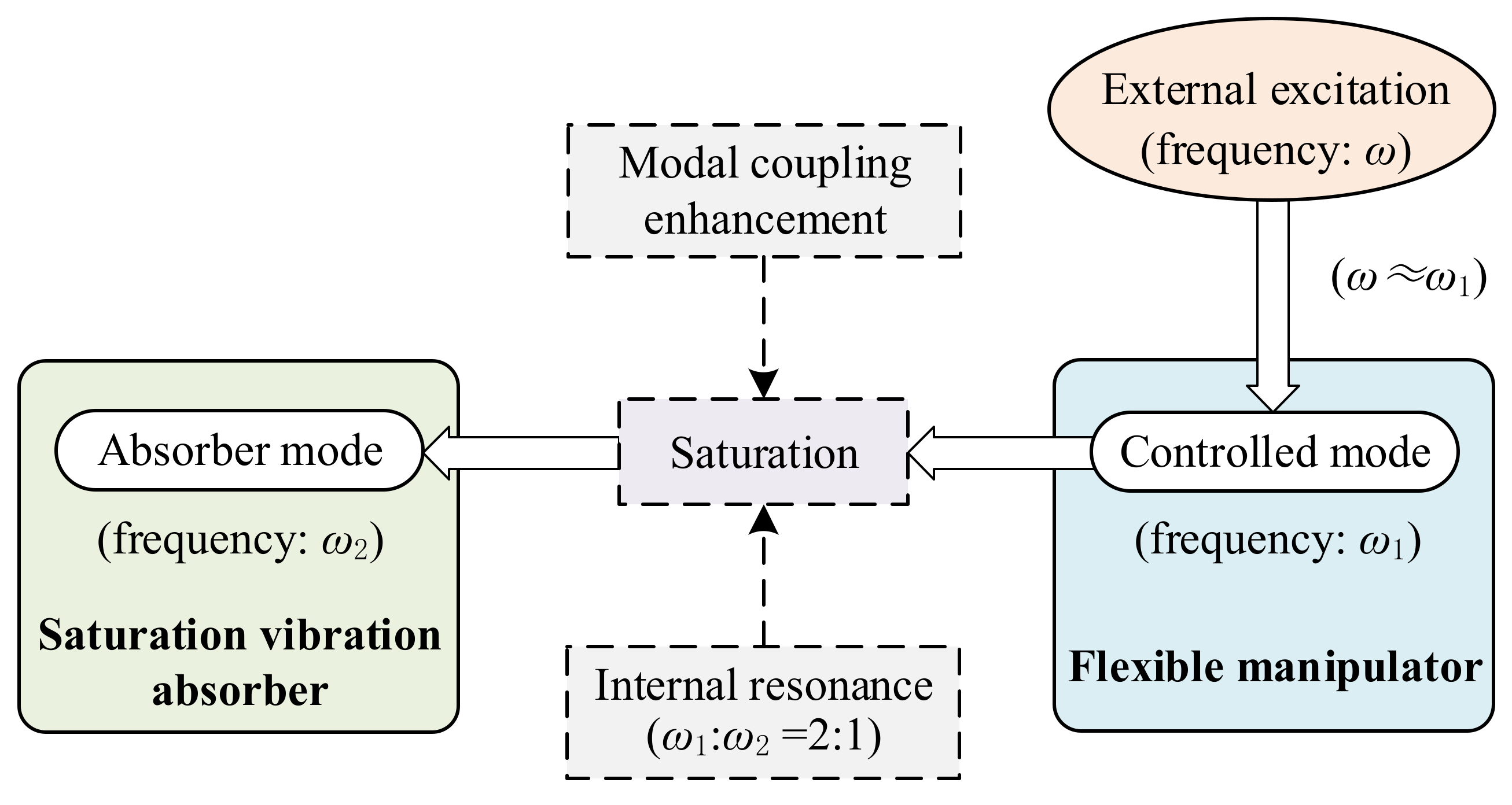
Inspired by the working principle of the saturation, a new primary resonance control scheme is put forward, as shown in Figure 2. A saturation-based vibration absorber is designed and mounted at the flexible manipulator to suppress the primary resonance. For the purpose of establishing an energy exchange channel for the saturation, 1:2 internal resonance is constructed between the mode of the vibration absorber and the controlled mode of the flexible manipulator. Moreover, a novel idea of modal coupling enhancement is proposed to improve saturation control performance by strengthening coupling relationship between the mode of the vibration absorber and the controlled mode of the flexible manipulator.

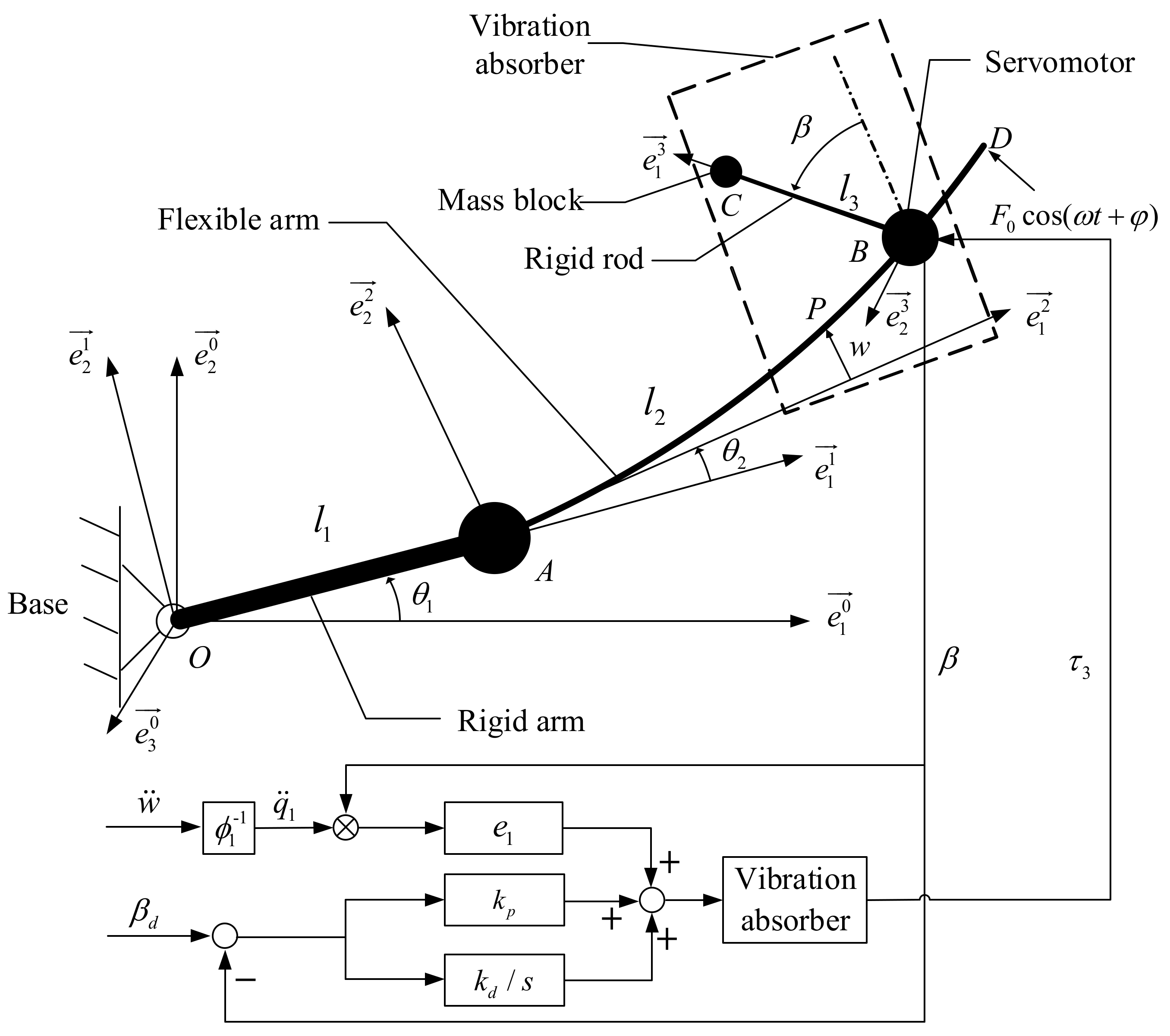
As shown in Figure 3, the suggested vibration absorber is mounted at point $B$ of the flexible manipulator, where $B\overrightarrow{e_1^3}\overrightarrow{e_2^3}$ is its moving coordinate system. The vibration absorber is composed of a rigid rod, a mass block, and a servomotor. The rigid rod is installed on the output shaft of the servomotor, whose angular displacement is denoted by $\beta$. The mass block is fixed at the end of the rigid rod to provide additional inertia. The servomotor plays an important role in the vibration absorber, whose control model is designed to establish the saturation by constructing 1:2 internal resonance and enhancing modal coupling.

To construct 1:2 internal resonance, the control torque signal ${\tau }_3$ of the servomotor is designed as

$${\tau }_3=k_p\left({\beta }^d-\beta \right)+k_d\left({\dot{\beta }}^d-\dot{\beta }\right),$$

(3)

where ${\beta }_{}^d$ and ${\dot{\beta }}_{}^d$ denote the desired angular displacement and the desired angular velocity of the rigid rod, respectively; $k_p$ and $k_d$ denote the position feedback gain coefficient and the speed feedback gain coefficient, respectively.

In order to work as a torsional vibration system, both ${\beta }_{}^d$ and ${\dot{\beta }}_{}^d$ are designated as zero. Therefore, Equation (3) becomes

$${\tau }_3=-k_p\beta -k_d\dot{\beta }.$$

(4)

Through adjusting $k_p$ and $k_d$, both the frequency and the damping of the vibration absorber are controlled to satisfy the requirement for establishing the saturation under 1:2 internal resonance.

Furthermore, for enhancing the modal coupling relationship between the vibration absorber and the flexible manipulator, a new nonlinear coupling term is constructed and introduced into the control torque signal ${\tau }_3$, i.e.,

$${\tau }_3=-k_p\beta -k_d\dot{\beta }+e_1{\ddot{q}}_1\beta ,$$

(5)

where $e_1$ denotes the coupling gain coefficient used to adjust coupling strength, and ${\ddot{q}}_1$ denotes the controlled modal coordinate acceleration of the flexible manipulator.

4. Dynamic Equations of Flexible Manipulator with Saturation-Based Vibration Absorber

In this study, ${\theta }_1(t)$ and ${\theta }_2(t)$ are predefined and implemented by joint servomotors. Therefore, the controlled mode coordinate $q_1$ of the flexible manipulator and the angular displacement $\beta$ of the vibration absorber are considered as the generalized coordinates. Using Kane’s method [3] and the Taylor expansion, the dynamic equations of the flexible manipulator with the suggested saturation-based vibration absorber are derived:

$$\begin{array}{l}{\ddot{q}}_1+2{\widehat{\zeta }}_1{\omega }_1{\dot{q}}_1+{\omega }_1^2{q}_1={\left({\dot{\theta }}_1+{\dot{\theta }}_2\right)}^2{q}_1-Q_1\left({\ddot{\theta }}_1+{\ddot{\theta }}_2\right)-Q_2\left({\dot{\theta }}_1{}^2{\theta }_2+{\ddot{\theta }}_1\right)+\\ Q_3\left[\beta \left({\ddot{\theta }}_1+{\ddot{\theta }}_2\right)+{\left({\dot{\theta }}_1+{\dot{\theta }}_2\right)}^2+\ddot{\beta }\beta +{\dot{\beta }}^2+2\dot{\beta }\left({\dot{\theta }}_1+{\dot{\theta }}_2\right)\right]+F_0^{*}\cos \left(\omega t+\phi \right),\end{array}$$

(6)

$$\begin{array}{l}\ddot{\beta }+2{\widehat{\zeta }}_2{\omega }_2\dot{\beta }+{\omega }_2^2\beta =-\left({\ddot{\theta }}_1+{\ddot{\theta }}_2\right)+P_1\left[\beta \left({\ddot{\theta }}_1+{\dot{\theta }}_1{}^2{\theta }_2\right)-{\dot{\theta }}_1{}^2+{\ddot{\theta }}_1{\theta }_2\right]+\\ P_2\left[\beta {\ddot{q}}_1-2{\dot{q}}_1\left({\dot{\theta }}_1+{\dot{\theta }}_2\right)-q_1\left({\ddot{\theta }}_1+{\ddot{\theta }}_2\right)-\beta q_1{\left({\dot{\theta }}_1+{\dot{\theta }}_2\right)}^2\right]+\\ P_3\left[\beta \left({\ddot{\theta }}_1+{\ddot{\theta }}_2\right)-{\left({\dot{\theta }}_1+{\dot{\theta }}_2\right)}^2\right]+e_1{\ddot{q}}_1\beta /m_C{l}_3^2,\end{array}$$

(7)

where ${\omega }_1^2=\frac{H_{22}}{L+m_C{\varphi }_{B1}{}^2+m_B{\varphi }_{B1}{}^2}$; ${\omega }_2^2=\frac{k_p}{m_C{l}_3^2}$; $2{\widehat{\zeta }}_1{\omega }_1=\frac{f_1}{L+m_C{\varphi }_{B1}{}^2+m_B{\varphi }_{B1}{}^2}$; $2{\widehat{\zeta }}_2{\omega }_2=\frac{k_d}{m_C{l}_3^2}$; $Q_1=\frac{F+\left(m_B+m_C\right){\varphi }_{B1}{x}_B}{L+m_C{\varphi }_{B1}{}^2+m_B{\varphi }_{B1}{}^2}$; $Q_2=\frac{m_B{\varphi }_{B1}{l}_1+L_0{l}_1+m_C{\varphi }_{B1}{l}_1}{L+m_C{\varphi }_{B1}{}^2+m_B{\varphi }_{B1}{}^2}$; $Q_3=\frac{m_C{\varphi }_{B1}{l}_3}{L+m_C{\varphi }_{B1}{}^2+m_B{\varphi }_{B1}{}^2}$; $F_0^{*}=\frac{F_0{\varphi }_{D1}}{L+m_C{\varphi }_{B1}{}^2+m_B{\varphi }_{B1}{}^2}$; $P_1=\frac{l_1}{l_3}$; $P_2=\frac{{\varphi }_{B1}}{l_3}$; $P_3=\frac{x_B}{l_3}$; $H_{22}={\displaystyle {\int }_0^{l_2}EI}\frac{d^4{\varphi }_1}{d{x}^4}{\varphi }_{1}dx$; $L_0={\displaystyle {\int }_0^{l_2}\rho {\varphi }_{1}dx}$; $L={\displaystyle {\int }_0^{l_2}\rho {\varphi }_1^{2}dx}$; $F={\displaystyle {\int }_0^{l_2}\rho {\varphi }_{1}xdx}$; $f_1$ is the natural damping of the flexible arm; ${\omega }_1^{}$, ${\omega }_2^{}$ and ${\omega }_{}^{}$ denote the frequencies of the flexible arm, the vibration absorber, and the external excitation, respectively; $l_1^{}$, $l_2^{}$, and $l_3^{}$ denote the lengths of the rigid arm, flexible arm, and rigid rod, respectively; $m_B$ and $m_C$ denote the masses of the joint $B$ and mass block, respectively; $\rho$ is the mass per length of the flexible arm; $x_B$ denotes the distance between $B$ and $A$ in the direction of $\overrightarrow{e_1^2}$ in the $A\overrightarrow{e_1^2}\overrightarrow{e_2^2}$; ${\varphi }_{B1}$ and ${\varphi }_{D1}$ are obtained when point $B$ and point $D$ are separately substituted into the controlled mode shape function ${\varphi }_1$; and $EI$ is the flexural rigidity of the flexible arm.

Equation (6) describes the forced vibration of the flexible manipulator, indicated by the controlled mode coordinate $q_1$ and the external excitation $F_0^{*}\cos \left(\omega t+\phi \right)$. If the external excitation frequency $\omega$ falls into the neighborhood of the controlled modal frequency ${\omega }_1^{}$ of the flexible manipulator, the primary resonance will occur and lead to a sharp increase in amplitude of the flexible manipulator. Because there is nonlinear coupling between $q_1$ and $\beta$, the vibration absorber can be used to suppress the primary resonance of the flexible manipulator. However, it should be noted that there is nonlinear coupling between flexible motion (indicated by $q_1$) and rigid motion (indicated by ${\theta }_1$ and ${\theta }_2$). Therefore, in the case of complex rigid–flexible motion coupling, whether the saturation can be established and utilized to suppress the primary resonance should be investigated.

Equation (7) describes the torsional vibration of the vibration absorber, indicated by the angular displacement $\beta$ of the vibration absorber. In Equation (7), the frequency ${\omega }_2^{}$ of the vibration absorber can be adjusted by the position feedback gain coefficient $k_p$. This feature will be used to establish the internal resonance between the flexible manipulator and the vibration absorber. Similarly, the damping ${\widehat{\zeta }}_2$ of the vibration absorber can be adjusted by the speed feedback gain coefficient $k_d$. This feature will be used to control the primary resonance of the flexible manipulator. In addition, $e_1$ will be used to adjust coupling strength between the mode $\beta$ of the vibration absorber and the controlled mode $q_1$ of the flexible manipulator for improving saturation control performance.

5. Internal Resonance Analysis

Because the saturation depends on the internal resonance, this section investigates the establishment of the internal resonance. For convenience of internal resonance analysis, the dimensionless parameters and scaling factor $0<\epsilon <<1$ are introduced into Equations (6) and (7) (See Appendix A). After omitting the higher-order terms containing ${\epsilon }^2$, Equations (6) and (7) become

$$\begin{array}{l}{\ddot{\widehat{q}}}_1+2\epsilon {\widehat{\zeta }}_1{\omega }_{S1}{\dot{\widehat{q}}}_1+{\omega }_{S1}^2{\widehat{q}}_1=-N_1\left({\ddot{\theta }}_1+{\ddot{\theta }}_2\right)-N_2{\ddot{\theta }}_1+\\ N_3\epsilon \left[\beta \left({\ddot{\theta }}_1+{\ddot{\theta }}_2\right)+{\left({\dot{\theta }}_1+{\dot{\theta }}_2\right)}^2+\ddot{\beta }\beta +{\dot{\beta }}^2+2\dot{\beta }\left({\dot{\theta }}_1+{\dot{\theta }}_2\right)\right]+\frac{\epsilon f_0^{*}}{l_1{\omega }_1^2}\cos \left({\omega }_{S3}\tau +\phi \right),\end{array}$$

(8)

$$\begin{array}{l}\ddot{\beta }+2\epsilon {\zeta }_2{\omega }_{S2}\dot{\beta }+{\omega }_{S2}^2\beta =-\left({\ddot{\theta }}_1+{\ddot{\theta }}_2\right)+S_1\epsilon \left[\beta {\ddot{\theta }}_1-{\dot{\theta }}_1{}^2+{\ddot{\theta }}_1{\theta }_2\right]+\\ S_2\epsilon \left[\beta {\ddot{\widehat{q}}}_1-2{\dot{\widehat{q}}}_1\left({\dot{\theta }}_1+{\dot{\theta }}_2\right)-{\widehat{q}}_1\left({\ddot{\theta }}_1+{\ddot{\theta }}_2\right)\right]+S_3\epsilon \left[\beta \left({\ddot{\theta }}_1+{\ddot{\theta }}_2\right)-{\left({\dot{\theta }}_1+{\dot{\theta }}_2\right)}^2\right]+\frac{\epsilon e_1{l}_1{\ddot{\widehat{q}}}_1\beta }{m_c{l}_3^2},\end{array}$$

(9)

where (˙) and (¨) denote the first-order and second-order derivatives concerning the dimensionless time $\tau$.

To seek the first-order approximate solutions of Equations (8) and (9), applying method of multiple scales [10] (see Appendix B) and separating the equations for each order of $\epsilon$ up to one yield:

Order (${\epsilon }^0$):

$$D_0^2{u}_0+{\omega }_{S1}^2{u}_0=-N_1\left(D_0^2{\theta }_1+D_0^2{\theta }_2\right)-N_2{D}_0^2{\theta }_1,$$

(10)

$$D_0^2{\beta }_0+{\omega }_{S2}{}^2{\beta }_0=-\left(D_0^2{\theta }_1+D_0^2{\theta }_2\right).$$

(11)

Order (${\epsilon }^1$):

$$\begin{array}{cc}\hfill & D_0^2{u}_1+{\omega }_{S1}^2{u}_1=N_3{\beta }_0\left(D_0^2{\theta }_1\right)+N_3{\beta }_0\left(D_0^2{\theta }_2\right)+N_3{\left(D_0{\theta }_1\right)}^2+2N_3\left(D_0{\theta }_1\right)\left(D_0{\theta }_2\right)+N_3{\left(D_0{\theta }_2\right)}^2+N_3\left(D_0^2{\beta }_0\right){\beta }_0+\hfill \\ \hfill & N_3{\left(D_0{\beta }_0\right)}^2+2N_3\left(D_0{\beta }_0\right)\left(D_0{\theta }_1\right)+2N_3\left(D_0{\beta }_0\right)\left(D_0{\theta }_2\right)-2{\zeta }_1{\omega }_{S1}{D}_0{u}_0-2D_1{D}_0{u}_0+\frac{f_0^{*}}{l_1{\omega }_1^2}cos \left({\omega }_{S3}{T}_0+\phi \right),\hfill \end{array}.$$

(12)

$$\begin{array}{cc}\hfill & D_0^2{\beta }_1+{\omega }_{S2}^2{\beta }_1=S_1\left[{\beta }_0{D}_0^2{\theta }_1+\left(D_0^2{\theta }_1\right){\theta }_2-{\left(D_0{\theta }_1\right)}^2\right]+S_3\left[{\beta }_0\left(D_0^2{\theta }_1+{D_0}^2{\theta }_2\right)-{\left(D_0{\theta }_1+D_0{\theta }_2\right)}^2\right]+\hfill \\ \hfill & S_2\left[{\beta }_0{D}_0^2{u}_0-u_0\left(D_0^2{\theta }_1+D_0^2{\theta }_2\right)-2\left(D_0{u}_0\right)\left(D_0{\theta }_1+D_0{\theta }_2\right)\right]-2{\zeta }_2{\omega }_{S2}{D}_0{\beta }_0-2D_0{D}_1{\beta }_0+\left(\frac{e_1{l}_1}{m_C{l}_3^2}\right)\left(D_0^2{u}_0·{\beta }_0\right).\hfill \end{array}$$

(13)

The expressions $D_0^2{\theta }_1$ and $D_0^2{\theta }_2$ in Equations (10) and (11) are linear in $T_0$, so the solutions of Equations (10) and (11) are expressed as

$$u_0=A_1{e}^{i{\omega }_{S1}{T}_0}+{\overline{A}}_1{e}^{-i{\omega }_{S1}{T}_0}-\left(N_1+N_2\right)D_0^2{\theta }_1-N_1{D}_0^2{\theta }_2,$$

(14)

$${\beta }_0=A_2{e}^{i{\omega }_{S2}{T}_0}+{\overline{A}}_2{e}^{-i{\omega }_{S2}{T}_0}-\left(D_0^2{\theta }_1+D_0^2{\theta }_2\right),$$

(15)

where $A_1$ and $A_2$ are complex functions of $T_1$, respectively; ${\overline{A}}_1$ and ${\overline{A}}_2$ are the conjugate of $A_1$ and $A_2$, respectively; and all of them are determined by the conditions of eliminating secular terms.

Substituting Equations (14) and (15) into Equations (12) and (13) can obtain solutions as follows:

$$D_0^2{u}_1+{\omega }_{S1}^2{u}_1=-\underset{¯}{2i{\zeta }_1{A}_1{\omega }_{S1}^2{e}^{i{\omega }_{S1}{T}_0}}-\underset{¯}{2i{A^{\prime }}_1{\omega }_{S1}{e}^{i{\omega }_{S1}{T}_0}}-\underset{¯}{2A_2^2{N}_3{\omega }_{S2}^2{e}^{2i{T}_0{\omega }_{S2}}}+\underset{¯}{\frac{1}{2}A{e}^{i\left({\omega }_{S3}{T}_0+\phi \right)}}+cc+NST,$$

(16)

$$\begin{array}{cc}\hfill & D_0^2{\beta }_1+{\omega }_{S2}^2{\beta }_1=-\underset{\_}{2i{\zeta }_2{A}_2{\omega }_{S2}^2{e}^{i{T}_0{\omega }_{S2}}}-\underset{\_}{2i{A}_2^{\prime }{\omega }_{S2}{e}^{i{T}_0{\omega }_{S2}}}+\underset{\_}{S_1{A}_2{e}^{i{T}_0{\omega }_{S2}}\left(D_0^2{\theta }_1\right)}+S_3\left[\underset{\_}{A_2{e}^{i{T}_0{\omega }_{S2}}\left(D_0^2{\theta }_1\right)}+\underset{\_}{A_2{e}^{i{T}_0{\omega }_{S2}}\left(D_0^2{\theta }_2\right)}\right]\hfill \\ \hfill & +{\tilde{S}}_2\left[-\underset{\_}{A_1{\overline{A}}_2{\omega }_{S1}^2{e}^{i{T}_0{\omega }_{S1}-i{T}_0{\omega }_{S2}}-}\underset{\_}{A_2{N}_1{e}^{i{T}_0{\omega }_{S2}}\left(D_0^4{\theta }_1\right)}-\underset{\_}{A_2{N}_2{e}^{i{T}_0{\omega }_{S2}}\left(D_0^4{\theta }_1\right)}-\underset{\_}{A_2{N}_1{e}^{i{T}_0{\omega }_{S2}}\left(D_0^4{\theta }_2\right)}\right]+cc+NST,\hfill \end{array}$$

(17)

where $cc$ denotes the complex conjugate of the preceding term, and $NST$ denotes secular term, $()\prime \equiv \partial ()/\partial T_1$,

$$A=\frac{f_0^{*}}{l_1{\omega }_1^2},$$

(18)

$${\tilde{S}}_2=S_2+\left(\frac{e_1{l}_1}{m_c{l}_3^2}\right).$$

(19)

In order to obtain the solutions of Equations (16) and (17), the solvability conditions are determined. Due to the primary resonance, the external excitation frequency is equal to the controlled modal frequency of the flexible manipulator, i.e., ${\omega }_{S3}={\omega }_{S1}$. In addition, 1:2 internal resonance condition is analyzed, because there are second-order nonlinear terms in Equations (8) and (9). Therefore, the detuning parameters ${\sigma }_1$ and ${\sigma }_2$ are introduced, i.e.,

$${\omega }_{S2}=0.5{\omega }_{S1}+\epsilon {\sigma }_1, {\omega }_{S3}={\omega }_{S1}+\epsilon {\sigma }_2.$$

(20)

Substituting Equation (20) into Equations (16) and (17) extracts the factors of $e^{i{T}_0{\omega }_{S1}}$ and $e^{i{T}_0{\omega }_{S2}}$, respectively. The solvability conditions can be obtained after eliminating the secular terms as follows:

$$2i{\zeta }_1{A}_1{\omega }_{S1}^2+2i{A}_1^{\prime }{\omega }_{S1}+2N_3{A}_2^2{\omega }_{S2}^2{e}^{2i{\sigma }_1{T}_1}-\frac{1}{2}A{e}^{i\left({\sigma }_2{T}_1+\phi \right)}=0,$$

(21)

$$\begin{array}{l}{S}_1{A}_2{D}_0^2{\theta }_1-{\tilde{S}}_2{A}_1{\overline{A}}_2{\omega }_{S1}^2{e}^{-2i{\sigma }_1{T}_1}-{\tilde{S}}_2{N}_1{A}_2{D}_0^4{\theta }_1-{\tilde{S}}_2{N}_2{A}_2{D}_0^4{\theta }_1-{\tilde{S}}_2{N}_1{A}_2{D}_0^4{\theta }_2\\ +S_3{A}_2\left[D_0^2{\theta }_1+D_0^2{\theta }_2\right]-2i{\zeta }_2{A}_2{\omega }_{S2}^2-2i{A^{\prime }}_2{\omega }_{S2}=0.\end{array}$$

(22)

For convenience, $A_1$ and $A_2$ in Equations (21) and (22) are rewritten in the form of polar coordinates as

$$A_1=\frac{1}{2}{a}_1{e}^{i{\alpha }_1}, A_2=\frac{1}{2}{a}_2{e}^{i{\alpha }_2},$$

(23)

where $a_1$ and $a_2$ denote the modal amplitudes of the flexible manipulator and the vibration absorber, respectively; ${\alpha }_1$ and ${\alpha }_2$ denote the phase angles; $a_1$, $a_2$, ${\alpha }_1$, and ${\alpha }_2$ are the real functions of $T_1$.

Substituting Equation (23) into Equations (21) and (22), then separating the result into real and imaginary parts, the steady-state solutions are obtained as follows:

$$a_1^{\prime }=-\frac{1}{2{\omega }_{S1}}{N}_3{a}_2^2{\omega }_{S2}^{2}sin {\gamma }_1-{\zeta }_1{a}_1{\omega }_{S1}^{}+\frac{1}{2{\omega }_{S1}}Asin {\gamma }_2,$$

(24)

$$a_2^{\prime }=\frac{1}{4{\omega }_{S2}}{\tilde{S}}_2{a}_2{a}_1{\omega }_{S1}^{2}sin {\gamma }_1-{\zeta }_2{a}_2{\omega }_{S2},$$

(25)

$$a_1{\alpha }_1^{\prime }=\frac{1}{2{\omega }_{S1}}{N}_3{a}_2^2{\omega }_{S2}^{2}cos {\gamma }_1-\frac{1}{2{\omega }_{S1}}Acos {\gamma }_2,$$

(26)

$$\begin{array}{l}{a}_2{{\alpha }^{\prime }}_2=\frac{1}{4{\omega }_{S2}}{\tilde{S}}_2{a}_2{a}_1{\omega }_{S1}^2\cos {\gamma }_1+\frac{1}{{\omega }_{S2}}\left(-\frac{1}{2}{S}_1{a}_2{D}_0^2{\theta }_1-\frac{1}{2}{S}_3{a}_2{D}_0^2{\theta }_1-\frac{1}{2}{S}_3{a}_2{D}_0^2{\theta }_2\right)\\ +\frac{1}{{\omega }_{S2}}\left(\frac{1}{2}{\tilde{S}}_2{N}_1{a}_2{D}_0^4{\theta }_1+\frac{1}{2}{\tilde{S}}_2{N}_2{a}_2{D}_0^4{\theta }_1+\frac{1}{2}{\tilde{S}}_2{N}_1{a}_2{D}_0^4{\theta }_2\right),\end{array}$$

(27)

where

$${\gamma }_1=2{\sigma }_1{T}_1+2{\alpha }_2-{\alpha }_1,$$

(28)

$${\gamma }_2={\sigma }_2{T}_1+\phi -{\alpha }_1.$$

(29)

According to Equations (26)–(29), one obtains

$$\begin{array}{cc}\hfill & {\gamma }_1^{\prime }=2{\sigma }_1+\frac{1}{2}\frac{{\tilde{S}}_2{a}_1{\omega }_{S1}^{2}cos {\gamma }_1}{{\omega }_{S2}}-\frac{S_1{D}_0^2{\theta }_1}{{\omega }_{S2}}-\frac{S_3{D}_0^2{\theta }_1}{{\omega }_{S2}}-\frac{S_3{D}_0^2{\theta }_2}{{\omega }_{S2}}+\frac{{\tilde{S}}_2{N}_1{D}_0^4{\theta }_1}{{\omega }_{S2}}\hfill \\ \hfill & +\frac{{\tilde{S}}_2{N}_2{D}_0^4{\theta }_1}{{\omega }_{S2}}+\frac{{\tilde{S}}_2{N}_1{D}_0^4{\theta }_2}{{\omega }_{S2}}-\frac{1}{2a_1{\omega }_{S1}^{}}{N}_3{\omega }_{S2}^2{a}_2^{2}cos {\gamma }_1+\frac{1}{2a_1{\omega }_{S1}^{}}Acos {\gamma }_2,\hfill \end{array}$$

(30)

$${\gamma }_2^{\prime }={\sigma }_2-\frac{1}{2a_1{\omega }_{S1}}{N}_3{\omega }_{S2}^2{a}_2^{2}cos {\gamma }_1+\frac{1}{2a_1{\omega }_{S1}}Acos {\gamma }_2.$$

(31)

Because the internal resonance is an internal channel used to exchange energy between the flexible manipulator and the vibration absorber, both the external excitation and the modal damping are not considered when analyzing the establishment of the internal resonance, i.e., $F=0$, $A=0$, and ${\zeta }_1={\zeta }_2=0$. In this case, dividing Equation (24) by Equation (25) obtains

$$a_1{a^{\prime }}_1=-v\cdot a_2{a^{\prime }}_2,$$

(32)

where

$$v=\frac{2N_3{\omega }_{S2}^3}{{\tilde{S}}_2}.$$

(33)

The integral of Equation (32) is

$$a_1^2+v{a}_2^2=E,$$

(34)

where $E$ is a constant of integration, which is proportional to the initial energy of the system; $a_1^2$ and $a_2^2$ represent the vibration energy of the flexible manipulator and the vibration absorber, respectively.

Substituting $N_3$ and ${\tilde{S}}_2$ into Equation (33), one obtains

$$v=\frac{2N_3{\omega }_{S2}^3}{{\tilde{S}}_2}=\frac{2{\omega }_{S2}^3{m}_C{\varphi }_{B1}{l}_3^2}{\left({\displaystyle {\int }_0^{l_2}\rho {\varphi }_1^{2}dx}+m_C{\varphi }_{B1}{}^2+m_B{\varphi }_{B1}{}^2\right)\left({\varphi }_{B1}+\frac{e_1}{m_C{l}_3}\right)l_1^2}.$$

(35)

If $v>0$, $a_1$ and $a_2$ are negatively correlated, as shown in Equation (34). It indicates that the internal resonance has been successfully established and the vibration energy is exchanging between the controlled mode of the flexible manipulator and the mode of the vibration absorber.

To realize $v>0$, $e_1$ in Equation (35) is solved and should satisfy the following condition:

$$\left\{e_1|e_1>-{\varphi }_{B1}{m}_c{l}_3,e_1\in R\right\}.$$

(36)

Through the above analysis, the generation condition of the internal resonance has been obtained. Based on 1:2 internal resonance, the saturation will be researched in the Section 6 for suppressing the primary resonance of the flexible manipulator.

6. Saturation Analysis

6.1. Steady-State Solutions of Primary Resonance

To reveal the saturation principle, the steady-state solutions of Equations (24) and (25), (30) and (31) need to be analyzed under the primary resonance and 1:2 internal resonance. Therefore, let the modal amplitude $a_i$ and the phase angle ${\gamma }_i$ in Equations (24) and (25), (30) and (31) no longer change with time (i.e., ${a^{\prime }}_1={a^{\prime }}_2=0$, ${{\gamma }^{\prime }}_1={{\gamma }^{\prime }}_2=0$).

Depending on whether the amplitude $a_2$ of the vibration absorber is zero, the steady-state solutions of $a_1$,$a_2$, ${\gamma }_1$, and ${\gamma }_2$ are divided into the following two cases: linear solutions and the nonlinear solutions.

Case 1 (linear solutions): $a_1\ne 0$ and $a_2=0$, i.e.,

$$a_1=\frac{A}{2{\omega }_{S1}}\sqrt{\frac{1}{{\zeta }_1^2{\omega }_{S1}^2+{\sigma }_2^2}},$$

(37)

$$a_2=0,$$

(38)

$$\tan {\gamma }_2=-\frac{{\zeta }_1{\omega }_{S1}}{{\sigma }_2},$$

(39)

$${\gamma }_1=arbitrary value.$$

(40)

Equations (37) and (38) show that the primary resonance amplitude $a_1$ of the flexible manipulator is linearly monotonically increasing with the amplitude $A$ of the external excitation, whereas the vibration absorber is not working. In this case, the saturation has not yet been established.

Case 2 (nonlinear solutions): $a_1\ne 0$ and $a_2\ne 0$, i.e.,

$$a_1=a_1^{*}=2\sqrt{{\left(\frac{\left({\Lambda }_1+2{\sigma }_1-{\sigma }_2\right)\left({\omega }_{S2}\right)}{{\tilde{S}}_2{\omega }_{S1}^2}\right)}^2+{\left(\frac{2{\zeta }_2{\omega }_{S2}^2}{{\tilde{S}}_2{\omega }_{S1}^2}\right)}^2}=\left|\frac{2{\omega }_{S2}}{{\tilde{S}}_2{\omega }_{S1}^2}\right|{\left({\left({\Lambda }_1+2{\sigma }_1-{\sigma }_2\right)}^2+{\left(2{\zeta }_2{\omega }_{S2}^{}\right)}^2\right)}^{1/2},$$

(41)

$$a_2=\sqrt{\frac{1}{2}\left(-{\Gamma }_1\pm \sqrt{{\Lambda }_2^2-{\Gamma }_2^2}\right)},$$

(42)

$$\tan {\gamma }_1=-\frac{2{\zeta }_2{\omega }_{S2}}{{\Lambda }_1+2{\sigma }_1-{\sigma }_2},$$

(43)

$$\tan {\gamma }_2=-\frac{2a_2^2{\zeta }_2{N}_3{\omega }_{S2}^4+a_1^2{\zeta }_1{\tilde{S}}_2{\omega }_{S1}^4}{a_1^2{\sigma }_2{\tilde{S}}_2{\omega }_{S1}^3+a_2^2{N}_3{\omega }_{S2}^3\left({\Lambda }_1+2{\sigma }_1-{\sigma }_2\right)},$$

(44)

$${\Lambda }_1=-\frac{S_1{D}_0^2{\theta }_1}{{\omega }_{S2}}-\frac{S_3{D}_0^2{\theta }_1}{{\omega }_{S2}}-\frac{S_3{D}_0^2{\theta }_2}{{\omega }_{S2}}+\frac{{\tilde{S}}_2{N}_1{D}_0^4{\theta }_1}{{\omega }_{S2}}+\frac{{\tilde{S}}_2{N}_2{D}_0^4{\theta }_1}{{\omega }_{S2}}+\frac{{\tilde{S}}_2{N}_1{D}_0^4{\theta }_2}{{\omega }_{S2}},$$

(45)

$${\Lambda }_2^{}=\frac{2A}{N_3^{}{\omega }_{S2}^2},$$

(46)

$${\Gamma }_1=\frac{8\left({\Lambda }_1{\sigma }_2-{\sigma }_2^2+2{\sigma }_1{\sigma }_2+2{\zeta }_1{\zeta }_2{\omega }_{S1}{\omega }_{S2}\right)}{N_3{\tilde{S}}_2{\omega }_{S1}{\omega }_{S2}},$$

(47)

$${\Gamma }_2^{}=\frac{8\left({\zeta }_1\left(-{\Lambda }_1\right){\omega }_{S1}+{\zeta }_1\left({\sigma }_2-2{\sigma }_1\right){\omega }_{S1}+2{\zeta }_2{\sigma }_2{\omega }_{S2}\right)}{N_3^{}{\tilde{S}}_2^{}{\omega }_{S1}^{}{\omega }_{S2}^{}}.$$

(48)

Equations (41) and (42) show that the vibration absorber is working, and the primary resonance amplitude $a_1$ of the flexible manipulator is not affected by the amplitude $A$ of the external excitation. It means that the primary resonance amplitude $a_1$ of the flexible manipulator will no longer increase with external excitation but maintain a constant value $a_1^{*}$; the rest of primary resonance energy will be transferred to the vibration absorber. These conclusions demonstrate the occurrence of saturation. In addition, $a_1^{*}$ denotes the primary resonance amplitude of the flexible manipulator when the saturation occurs, and thus is called the saturation amplitude in this study. A smaller $a_1^{*}$ means more primary resonance energy has been transferred to the vibration absorber via the internal resonance. Therefore, $a_1^{*}$ is an important index evaluating saturation control performance.

It should be noted that the amplitude $a_2$ of the vibration absorber in Equation (42) is not unique, and is determined by ${\Lambda }_2^{}$ and ${\Gamma }_1$. To ensure $a_2$ has real solutions, two critical values of ${\Lambda }_2^{}$ are obtained by the following boundary conditions:

$${\Lambda }_{2-1}^{}=\left|{\Gamma }_2^{}\right|, {\Lambda }_{2-2}^{}=\sqrt{{\Gamma }_1^2+{\Gamma }_2^2}.$$

(49)

From Equation (49), the critical values of $f_0^{*}$ are derived, i.e.,

$$f_0^{*}={\xi }_1=\frac{{\omega }_2^2{N}_3{l}_1}{2}\left|{\Gamma }_2\right|, f_0^{*}={\xi }_2=\frac{{\omega }_2^2{N}_3{l}_1}{2}{\left|{\Gamma }_1^2+{\Gamma }_2^2\right|}^{1/2},$$

(50)

where ${\xi }_2>{\xi }_1$.

Depending on ${\Gamma }_1\ge 0$ or ${\Gamma }_1<0$, the real solutions of $a_2$ associated with different external excitation $f_0^{*}$ are discussed as follows.

For ${\Gamma }_1\ge 0$, if $f_0^{*}>{\xi }_2$, then $a_2$ has one nonlinear solution:

$$a_2=\sqrt{\frac{1}{2}\left(-{\Gamma }_1+\sqrt{{\Lambda }_2^2-{\Gamma }_2^2}\right)}.$$

(51)

For ${\Gamma }_1<0$, if ${\xi }_1<f_0^{*}<{\xi }_2$, then $a_2$ has two nonlinear solutions:

$$a_2=\sqrt{\frac{1}{2}\left(-{\Gamma }_1+\sqrt{{\Lambda }_2^2-{\Gamma }_2^2}\right)},$$

(52)

$$a_2=\sqrt{\frac{1}{2}\left(-{\Gamma }_1-\sqrt{{\Lambda }_2^2-{\Gamma }_2^2}\right)}.$$

(53)

For ${\Gamma }_1<0$, if $f_0^{*}>{\xi }_2$, then $a_2$ has one nonlinear solution:

$$a_2=\sqrt{\frac{1}{2}\left(-{\Gamma }_1+\sqrt{{\Lambda }_2^2-{\Gamma }_2^2}\right)}.$$

(54)

There are no solutions in other cases.

6.2. Saturation Principle

According to Section 6.1, the steady-state solutions of the primary resonance consist of the linear solutions and nonlinear solutions. The former indicates that the saturation has not been established, and the latter indicates that the saturation has been established. Whether the saturation can be successfully established depends on the stability of these solutions. Therefore, the saturation principle is revealed in this section by way of stability analysis.

For this purpose, the determinant of the Jacobian matrix $\left[\mathit{J}\right]$ (See Appendix C for the process) is

$$\left|\mathit{J}\right|=\left|\begin{array}{cccc}-{\zeta }_1{\omega }_{S1}^{}\hfill & -{\sigma }_2\hfill & \frac{1}{{\omega }_{S1}}{N}_3{\omega }_{S2}^2{y}_2\hfill & \frac{1}{{\omega }_{S1}}{N}_3{\omega }_{S2}^2{x}_2\hfill \\ {\sigma }_2\hfill & -{\zeta }_1{\omega }_{S1}^{}\hfill & -\frac{1}{{\omega }_{S1}}{N}_3{\omega }_{S2}^2{x}_2^{}\hfill & \frac{1}{{\omega }_{S1}}{N}_3{\omega }_{S2}^2{y}_2^{}\hfill \\ -\frac{1}{4{\omega }_{S2}}{\tilde{S}}_2{\omega }_{S1}^2{y}_2\hfill & \frac{1}{4{\omega }_{S2}}{\tilde{S}}_2{\omega }_{S1}^2{x}_2\hfill & A_{33}\hfill & A_{34}\hfill \\ -\frac{1}{4{\omega }_{S2}}{\tilde{S}}_2{\omega }_{S1}^2{x}_2\hfill & -\frac{1}{4{\omega }_{S2}}{\tilde{S}}_2{\omega }_{S1}^2{y}_2\hfill & A_{43}\hfill & A_{44}\hfill \end{array}\right|,$$

(55)

where

$$\left\{\begin{array}{l}{A}_{33}=-{\zeta }_2{\omega }_{S2}^{}+\frac{1}{4{\omega }_{S2}}{\tilde{S}}_2{\omega }_{S1}^2{y}_1\\ A_{34}=\frac{1}{2}\left({\Lambda }_1-{\sigma }_2+2{\sigma }_1\right)-\frac{1}{4{\omega }_{S2}}{\tilde{S}}_2{\omega }_{S1}^2{x}_1\\ A_{43}=-\frac{1}{2}\left({\Lambda }_1-{\sigma }_2+2{\sigma }_1\right)-\frac{1}{4{\omega }_{S2}}{\tilde{S}}_2{\omega }_{S1}^2{x}_1\\ A_{44}=-{\zeta }_2{\omega }_{S2}^{}-\frac{1}{4{\omega }_{S2}}{\tilde{S}}_2{\omega }_{S1}^2{y}_1.\end{array}\right.$$

(56)

For the linear solutions, the eigenvalues of $\left|\mathit{J}\right|$ are obtained as follows:

$${\lambda }_{1,2}=\frac{-4{\zeta }_2{\omega }_{S2}^2\pm \sqrt{{\tilde{S}}_2^2{\omega }_{S1}^4{a}_1^2-4{\left({\Lambda }_1+2{\sigma }_1-{\sigma }_2\right)}^2{\omega }_{S2}^2}}{4{\omega }_{S2}}, {\lambda }_{3,4}=-{\zeta }_1{\omega }_{S1}\pm i\left|{\sigma }_2\right|.$$

(57)

The linear solutions are stable if the real parts of Equation (57) are negative. Thus, the stable condition of the linear solutions is

$$a_1<a_1^{*}=\left|\frac{2{\omega }_{S2}}{{\tilde{S}}_2{\omega }_{S1}^2}\right|{\left({\left({\Lambda }_1+2{\sigma }_1-{\sigma }_2\right)}^2+{\left(2{\zeta }_2{\omega }_{S2}^{}\right)}^2\right)}^{1/2}.$$

(58)

Equation (58) indicates that the linear solutions are stable if the primary resonance amplitude $a_1$ of the flexible manipulator is less than the saturation amplitude $a_1^{*}$. In this case, the vibration absorber is not working, and the saturation is not established.

For the nonlinear solutions, the characteristic equation of the Jacobian matrix $\left|\mathit{J}\right|$ is defined as

$${\lambda }^4+{\delta }_1{\lambda }^3+{\delta }_2{\lambda }^2+{\delta }_3\lambda +{\delta }_4=0,$$

(59)

where $\lambda$ denotes the eigenvalue of $\left|\mathit{J}\right|$; ${\delta }_1$, ${\delta }_2$, ${\delta }_3$, and ${\delta }_4$ denote the factors of the characteristic equation as shown in Appendix D.

Based on the Routh–Hurwitz criterion [27], the nonlinear solutions are stable under the following conditions:

$$\left\{\begin{array}{l}{\delta }_1>0\hfill \\ {\delta }_1{\delta }_2-{\delta }_3>0\hfill \\ {\delta }_3\left({\delta }_1{\delta }_2-{\delta }_3\right)-{\delta }_1^2{\delta }_4>0\hfill \\ {\delta }_4>0.\hfill \end{array}\right.$$

(60)

In this case, the vibration absorber is working, and the saturation is established.

From Equations (A14)–(A17), it can be seen that the stability of the nonlinear solutions is affected by several important parameters, including ${\sigma }_1$, ${\sigma }_2$, $k_d$, $e_1$, ${\Lambda }_1$, $a_1$, and $a_2$. Therefore, Equation (60) will be used to search a reasonable range of these parameters for establishing the saturation.

Above stability analyses on the steady-state solutions of the primary resonance have revealed the saturation principle. In the Section 6.3, a numerical example will be used to verify the saturation principle.

6.3. Verification of Saturation Principle

In this section, an example is used to verify the saturation principle. The damping coefficient of the flexible manipulator is ${\widehat{\zeta }}_1=0.0005$; $k_p=0.67$ is determined according to the internal resonance relationship ($w_1:w_2\approx 2:1$); $k_d=0.0005$ and $e_1=0$ are selected according to Equation (60). The other structural parameters of the flexible manipulator and the vibration absorber are listed in

Table 1. Structural parameters of the flexible manipulator and vibration absorber.

Components	Parameters
Rigid arm	$\mathrm{Length} l_1=0.4 \mathrm{m}$$, \mathrm{Sec}\mathrm{tion} \mathrm{width} b_1=0.07 \mathrm{m}$$, \mathrm{Sec}\mathrm{tion} \mathrm{height} h_1=0.05 \mathrm{m}$$, \mathrm{Mass} m_1=2.8 \mathrm{kg}$
Flexible arm	$\mathrm{Length} l_2=0.8 \mathrm{m}$$, \mathrm{Sec}\mathrm{tion} \mathrm{width} b_2=0.005 \mathrm{m}$$, \mathrm{Sec}\mathrm{tion} \mathrm{height} h_2=0.03 \mathrm{m}$, $\mathrm{Density} {\rho }_1=7.8\times {10}^3 \mathrm{kg}/{\mathrm{m}}^3$$, \mathrm{Linear} \mathrm{density} \rho =1.17 \mathrm{kg}/\mathrm{m}$, $\mathrm{Polar} \mathrm{moment} \mathrm{of} \mathrm{inertia} I=3.125\times {10}^{-10} {\mathrm{m}}^4$$, \mathrm{Modulus} \mathrm{of} \mathrm{elasticity} E=2.1\times {10}^{11} \mathrm{Pa}$
Joint A	$\mathrm{Mass} m_A=3.55 \mathrm{kg}$
Joint B	$\mathrm{Mass} m_B=0.65 \mathrm{kg}$
Rigid rod	$\mathrm{Length} l_3=0.3 \mathrm{m}$, Cross-section diameter $d=0.008 \mathrm{m}$, Density ${\rho }_2=7.8\times {10}^3 \mathrm{kg}/{\mathrm{m}}^3$
Mass block	$\mathrm{Mass} m_C=0.04 \mathrm{kg}$

.

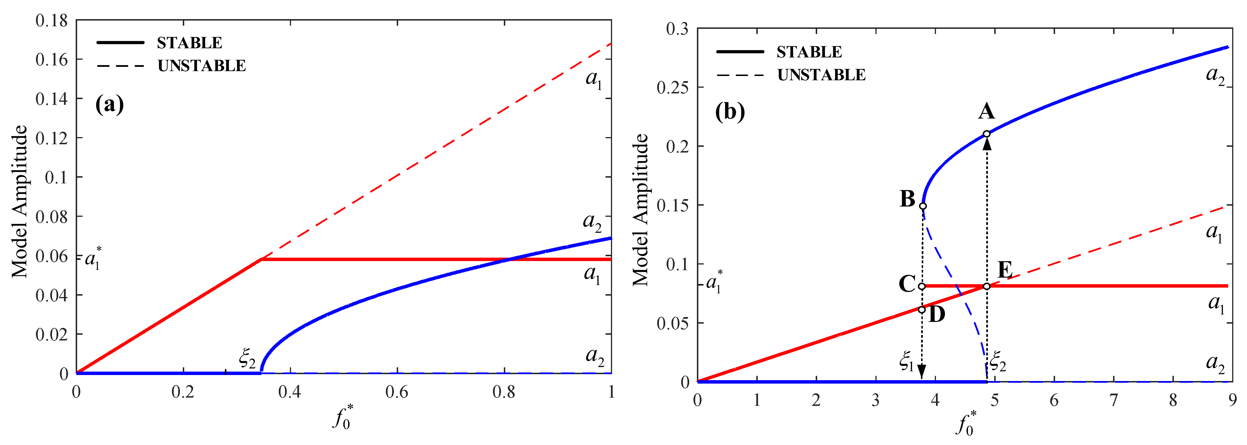
According to whether the primary resonance is ideally tuned, two cases are discussed. If both the internal resonance and the primary resonance are ideally tuned, i.e., ${\sigma }_1=0$ and ${\sigma }_2=0$, then ${\Gamma }_1>0$ in Equation (47). As shown in Figure 4a, with the increase of the external excitation amplitude $f_0^{*}$ from zero, the controlled modal amplitude $a_1$ of the flexible manipulator increases linearly, whereas the modal amplitude $a_2$ of the vibration absorber remains at zero. This result agrees with the linear solution Equations (37) and (38) of the primary resonance. The input energy has excited the primary resonance of the flexible manipulator but has not been transferred to the vibration absorber. In this case, the saturation does not occur. However, if $f_0^{*}>{\xi }_2$, the modal amplitude $a_2$ of the vibration absorber will increase, and the controlled modal amplitude $a_1$ of the flexible manipulator will no longer increase and maintain a constant value (i.e., the saturation amplitude $a_1^{*}$). This is because the linear solutions given by Equations (37) and (38) become unstable, whereas the nonlinear solutions given by Equations (41) and (42) become stable. As ${\Gamma }_1>0$ and $f_0^{*}>{\xi }_2$, Equation (42) becomes Equation (51). These results show that the saturation has been established, and the rest of primary resonance energy has been transferred to the vibration absorber.

If the internal resonance is ideally tuned and the primary resonance is not ideally tuned, such as ${\sigma }_1=0$ and ${\sigma }_2=0.1$, then ${\Gamma }_1<0$ in Equation (47). As shown in Figure 4b, if ${\xi }_1<f_0^{*}<{\xi }_2$, with the increase of the external excitation amplitude $f_0^{*}$ from zero, the controlled modal amplitude $a_1$ of the flexible manipulator increases linearly, whereas the modal amplitude $a_2$ of the vibration absorber remains at zero. This result agrees with the linear solution Equations (37) and (38) of the primary resonance. When $f_0^{*}$ reaches ${\xi }_2$, however, the jump phenomena will arise. The value of $a_1$ remains the constant value $a_1^{*}$, and $a_2$ jumps from zero to A. Similarly, when $f_0^{*}$ decreases to ${\xi }_1$, $a_1$ jumps from C to D, and $a_2$ jumps from B to zero. These phenomena agree with Equations (52) and (53). When $f_0^{*}>{\xi }_2$, the stable solution $a_1$ is equal to $a_1^{*}$, which is independent of the amplitude $f_0^{*}$ of the external excitation. It indicates that the saturation has been established. As a result, ${\xi }_2$ at which the controlled modal amplitude of the flexible manipulator reaches saturation is called the external excitation threshold in this study. A smaller $f_0^{*}$ means that the saturation is easier to establish. Therefore, $f_0^{*}$ is an important index for evaluating saturation control performance.

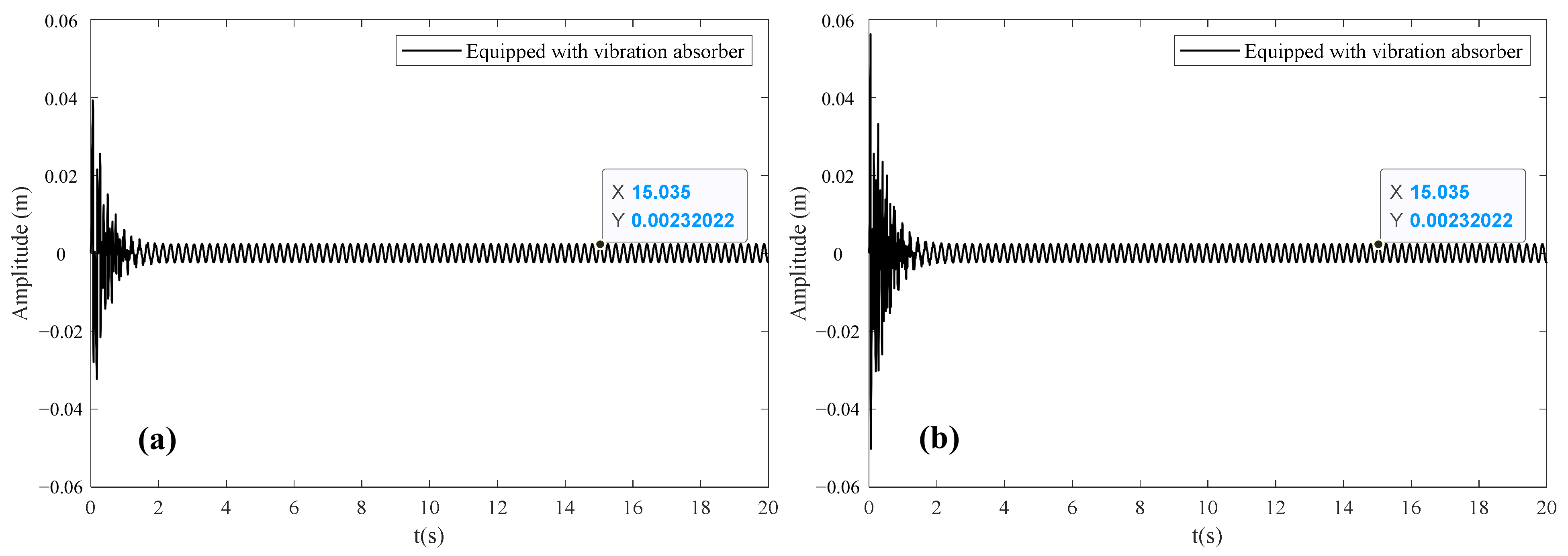
In order to further exhibit the saturation phenomenon, numerical simulations are conducted to show the saturation amplitudes of the flexible manipulator under external excitations amplitudes of $0.05 \mathrm{N}$ and $0.1 \mathrm{N}$, respectively. As shown in Figure 5, the steady saturation amplitudes of the flexible manipulator under different excitations no longer increase and remain $0.0023 \mathrm{m}$ under saturation control. It indicates that saturation has been established and primary resonance amplitude has been effectively suppressed without increasing anymore.

In conclusion, with the increase of the external excitation amplitude $f_0^{*}$ from zero, the controlled modal amplitude $a_1$ of the flexible manipulator is excited and gradually increases, whereas the modal amplitude $a_2$ of the vibration absorber is not yet excited and remains at zero. When $f_0^{*}$ reaches ${\xi }_2$, $a_1$ increases to the saturation amplitude $a_1^{*}$. Subsequently, the linear solutions become unstable and the nonlinear solutions become stable. If $f_0^{*}>{\xi }_2$, then the modal amplitude $a_2$ of the vibration absorber will increase, and the controlled modal amplitude $a_1$ of the flexible manipulator will no longer increase but maintain a constant value $a_1^{*}$. It means that the saturation has been established, and the rest of primary resonance energy has been transferred to the vibration absorber.

6.4. Effectiveness Analysis of Saturation Control

As stated above, the saturation depends on the establishment of the internal resonance. However, if the 1:2 internal resonance condition cannot be satisfied, indicated by the detuning parameter ${\sigma }_1$ in Equation (20), whether the saturation can be established should be researched. In addition, if the external excitation frequency slightly differs from the controlled modal frequency of the flexible manipulator, indicated by the detuning parameter ${\sigma }_2$ in Equation (20), whether the saturation can be established should be researched. For this purpose, the effect of ${\sigma }_1$ and ${\sigma }_2$ on saturation control is analyzed. Let $\omega =27.28 \mathrm{rad}/\mathrm{s}$, $F_0=0.05 \mathrm{N}$, $\phi =0$, ${\widehat{\zeta }}_1=5\times {10}^{-4}$, $k_d=5\times {10}^{-4}$, and $e_1=0$.

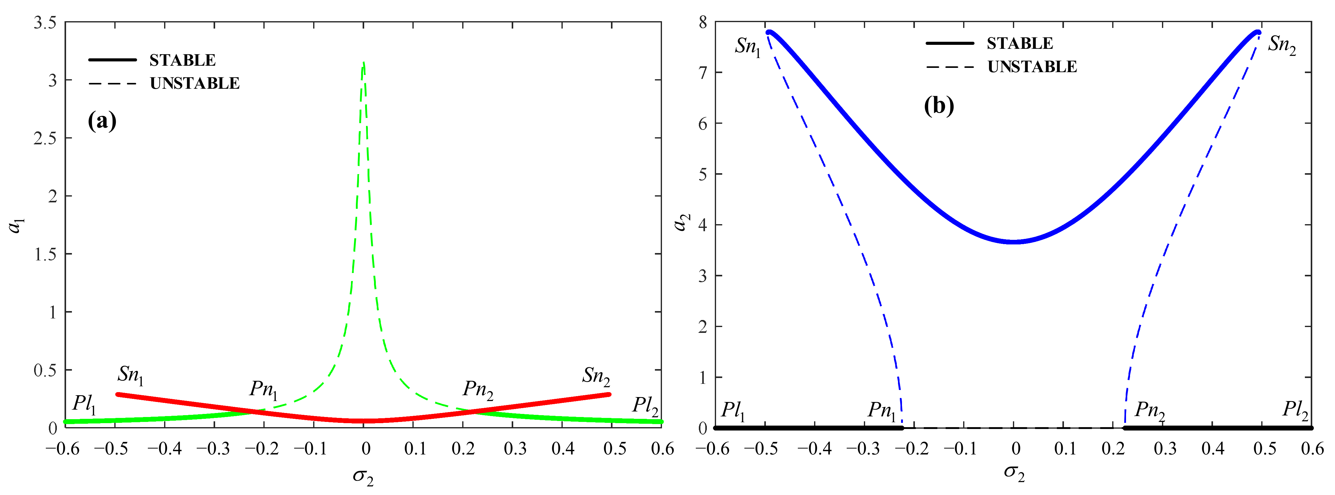
Case 1: 1:2 internal resonance condition is satisfied (i.e., ${\sigma }_1=0$) and the primary resonance is detuned (for example, ${\sigma }_2$ is in $\left[-0.6,0.6\right]$). As shown in Figure 6, the green and red lines represent the controlled modal amplitude $a_1$ of the flexible manipulator when the vibration absorber is inactive and active, respectively; the black and blue lines represent the modal amplitude $a_2$ of the vibration absorber in inactive and active state, respectively; and the solid and dotted lines represent the stable or unstable amplitude. When ${\sigma }_2\in \left[P{n}_1,P{n}_2\right]$, the nonlinear solutions are stable and the linear solutions are unstable. In this case, the primary resonance can be suppressed by the saturation. Therefore, $\left[P{n}_1,P{n}_2\right]$ is called the saturation control bandwidth in this study. Obviously, increasing the saturation control bandwidth can improve the effectiveness of the suggested saturation control method. Therefore, the saturation control bandwidth is an important index evaluating saturation control performance.

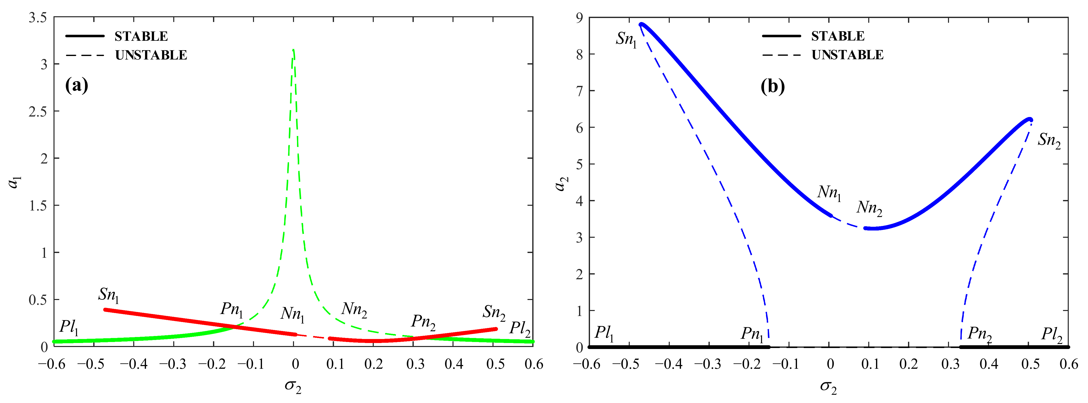
Case 2: 1:2 internal resonance condition is not satisfied (for example, ${\sigma }_1=0.1$) and the primary resonance is detuned (for example, ${\sigma }_2$ is in $\left[-0.6,0.6\right]$). As shown in Figure 7, when ${\sigma }_2\in \left[P{n}_1,N{n}_1\right]$ or ${\sigma }_2\in \left[N{n}_2,P{n}_2\right]$, the nonlinear solutions are stable and the linear solutions are unstable. In this case, the primary resonance can be suppressed by the saturation. However, $\left[N{n}_1,N{n}_2\right]$ is an unstable region, within which both the nonlinear solutions and the linear solutions are unstable. In this case, the saturation cannot be successfully established.

In conclusion, when 1:2 internal resonance condition is not satisfied, the saturation may not be successfully established in some cases. Therefore, the frequency of the suggested vibration absorber is designed to be adjustable to satisfy the requirement for establishing 1:2 internal resonance.

7. Configuration of Saturation Vibration Absorber

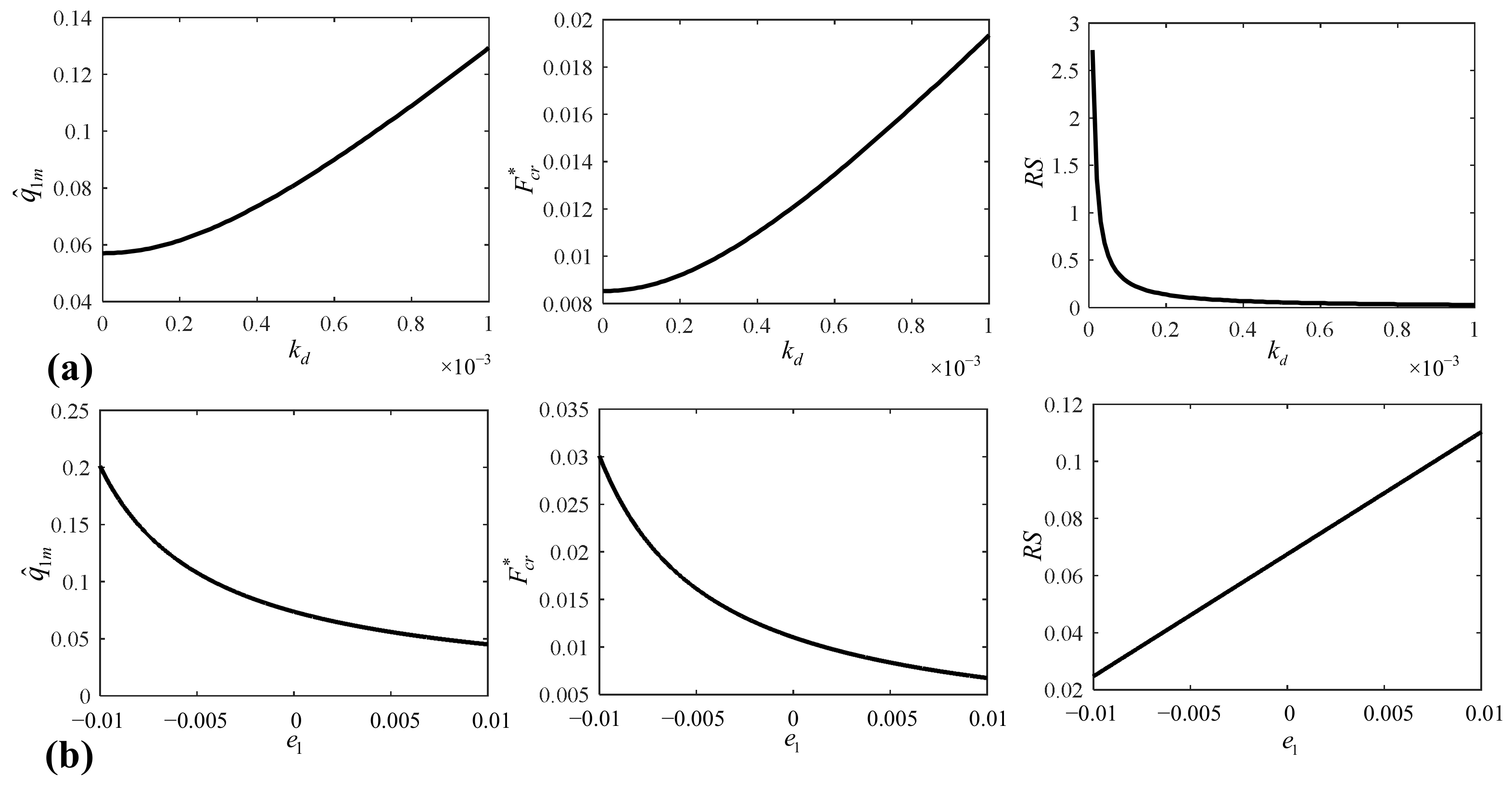
According to the analysis of Section 6, saturation control performance is mainly determined by the saturation amplitude, the external excitation threshold, and the saturation control bandwidth. For the convenience of describing the influence of the vibration absorber configuration parameters on saturation control performance, the saturation amplitude, the external excitation threshold, and the saturation control bandwidth are simplified as follows:

$${\widehat{q}}_{1m}=\left|\frac{1}{{\tilde{S}}_2}\right|{\left({\left(\left(1-\frac{\omega }{2{\omega }_2}\right)\right)}^2+{\widehat{\zeta }}_2^2\right)}^{1/2},$$

(61)

$$F_{cr}^{*}=\frac{8{\omega }_2^2{l}_1}{{\tilde{S}}_2}{\left({\left(\left(1-\frac{{\omega }_{S3}}{2{\omega }_{S2}}\right)\epsilon {\sigma }_2+{\widehat{\zeta }}_1{\widehat{\zeta }}_2\right)}^2+{\left({\widehat{\zeta }}_1\left(1-\frac{{\omega }_{S3}}{2{\omega }_{S2}}\right)+{\widehat{\zeta }}_2\epsilon {\sigma }_2\right)}^2\right)}^{1/2}$$

(62)

$$RS=2\sqrt{\left[{\left(\frac{{\tilde{S}}_2{F}_0^{*}}{8l_1{\omega }_2^2{\widehat{\zeta }}_2}\right)}^2-{\widehat{\zeta }}_1{}^2\right]},$$

(63)

where ${\widehat{q}}_{1m}$ denotes the dimensionless saturation amplitude, $F_{cr}^{*}$ denotes the dimensionless external excitation threshold, and $RS$ denotes the saturation control bandwidth.

Obviously, smaller $a_1^{*}$, smaller ${\xi }_2$, and larger $RS$ mean better saturation control performance. From Equations (61)–(63), it can be concluded that both the structural parameters (i.e., $l_3$, $m_C$, $x_B$) and the control parameters (i.e., $k_d$, $e_1$) of the vibration absorber can affect these indexes. As the structural parameters are difficult to change, this section will discuss how to configure the speed feedback gain coefficient $k_d$ and the coupling gain coefficient $e_1$ of the vibration absorber to improve saturation control performance.

Let $\omega =27.28 \mathrm{rad}/\mathrm{s}$, $F_0=0.05 \mathrm{N}$, $\phi =0$, and ${\widehat{\zeta }}_1=$ 5 × 10⁻⁴. As shown in Figure 8a, when $e_1=0$, with the increase of $k_d$, both ${\widehat{q}}_{1m}$ and $F_{cr}^{*}$ increase, but $RS$ decreases. Therefore, decreasing $k_d$ while satisfying the formula (60) can improve saturation control performance. As shown in Figure 8b, when $k_d=0.0005$, with the increase of $e_1$, both ${\widehat{q}}_{1m}$ and $F_{cr}^{*}$ decrease, but $RS$ increases. Therefore, increasing $e_1$ while satisfying the Formula (60) can improve saturation control performance.

8. Virtual Prototyping Simulation

Although the above analysis conclusions are promising, they are based on our own theoretical model. For this reason, three well-known software packages, i.e., ADAMS^® (Los Angeles, CA, USA), ANSYS^® (Canonsburg, PA, USA), and MATLAB^® (Natick, MA, USA), are employed in this section to conduct a series of virtual prototyping simulations. Because they implement dynamic modeling and vibration analysis in different ways from us, more trusted results can be obtained to verify our work.

8.1. Simulation Model

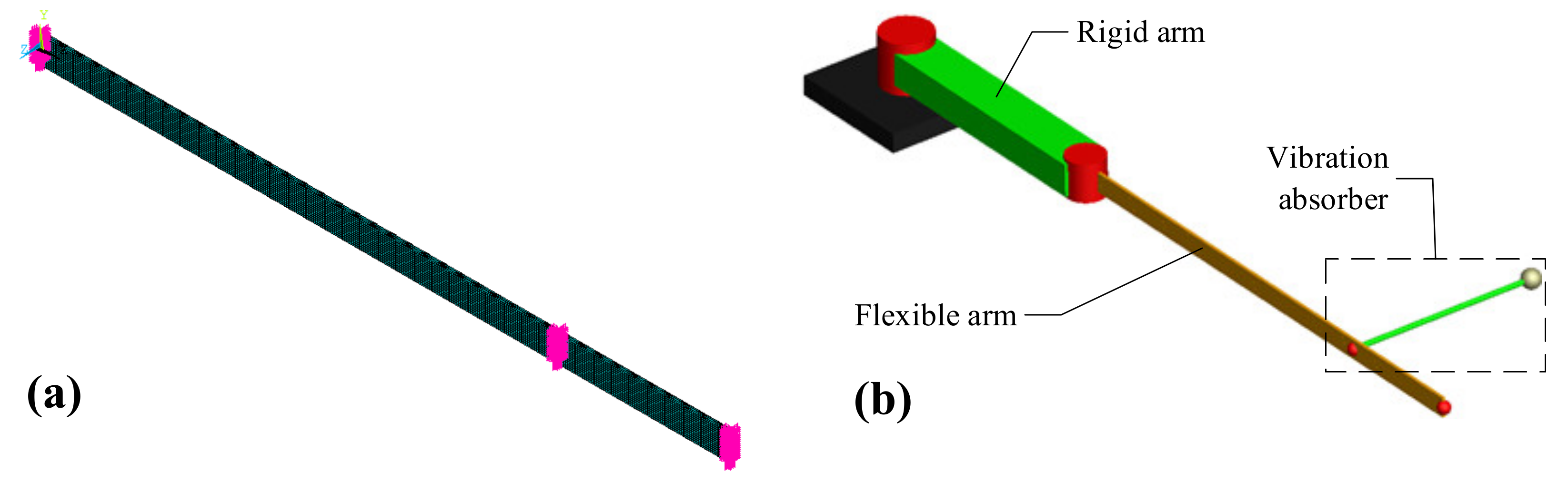
The finite element model of the flexible arm is established using ANSYS software, as shown in Figure 9a. With the help of ADAMS software, the multi-body dynamic model of a two-link manipulator and a saturation-based vibration absorber is established by importing the neutral file exported from the finite element model, as shown in Figure 9b. The detailed parameters of the model are listed in Table 1.

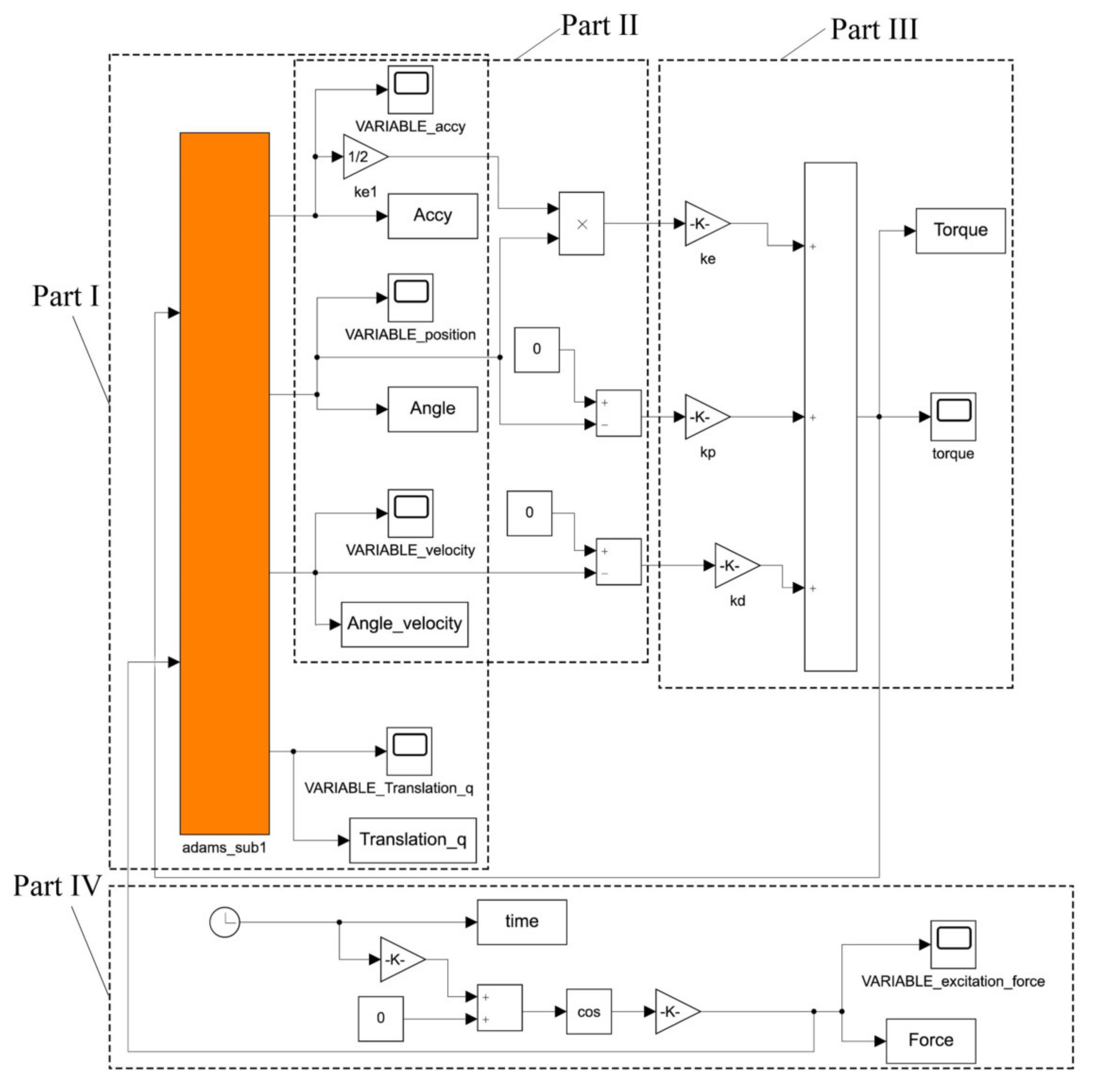
The suggested saturation control model is implemented based on the ADAMS/Control module and the MATLAB/Simulink module. As shown in Figure 10, part Ⅰ is the data interface module used to output the displacement, the speed, and acceleration signals measured in ADAMS software to the feedback controller module (i.e., part Ⅱ) of the vibration absorber. In part Ⅱ, according to the signals of part Ⅰ, both the linear and nonlinear feedback control are realized by adjusting the position feedback gain coefficient $Kp$, the speed feedback gain coefficient $Kd$, and the coupling gain coefficient $Ke$. Part Ⅲ represents the servomotor output torque modulated by part Ⅱ. Part Ⅳ is the external excitation analog signal module.

8.2. Simulation Analysis on Saturation Control

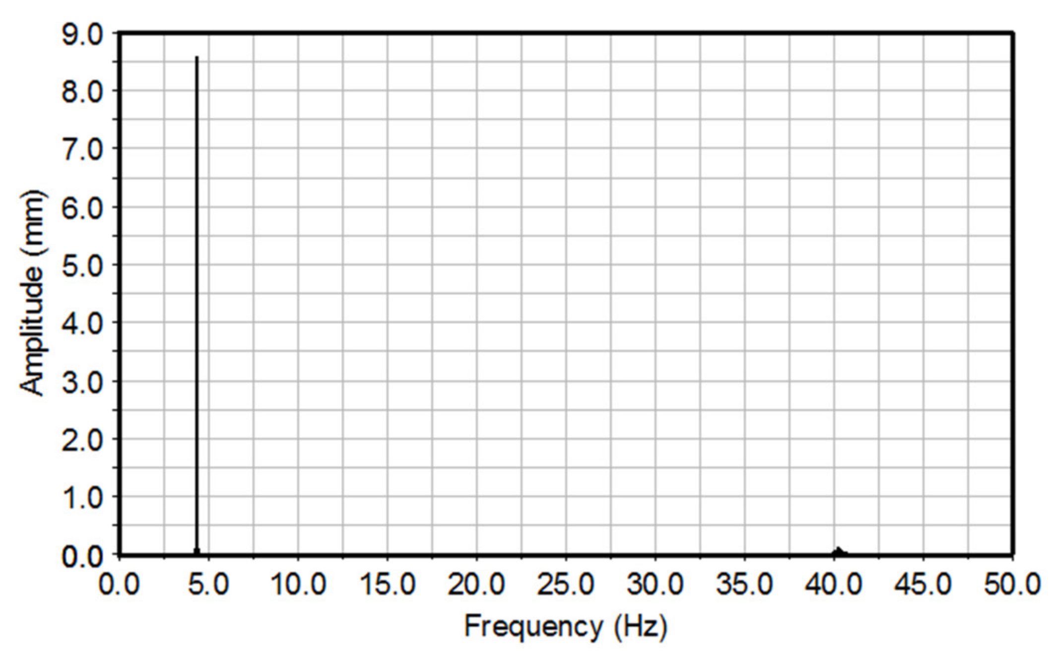
The effect of the speed feedback gain coefficient $Kd$ and the coupling gain coefficient $Ke$ on saturation control is researched. The simulation analysis is carried out when both the primary resonance and internal resonance are completely tuned (i.e., ${\sigma }_1=0$, ${\sigma }_2=0$). Figure 11 shows that the first-order natural frequency of the flexible arm is $4.3457 \mathrm{Hz}$. According to Equation (20) and ${\omega }_2^2=k_p/m_C{l}_3^2$, we have $Kp=670$. The initial value of the external excitation $F=F_0\cos \left(\omega t+\phi \right)$ is $\omega =27.28 \mathrm{rad}/\mathrm{s}$,$F_0=0.05 \mathrm{N}$,$\phi =0$.

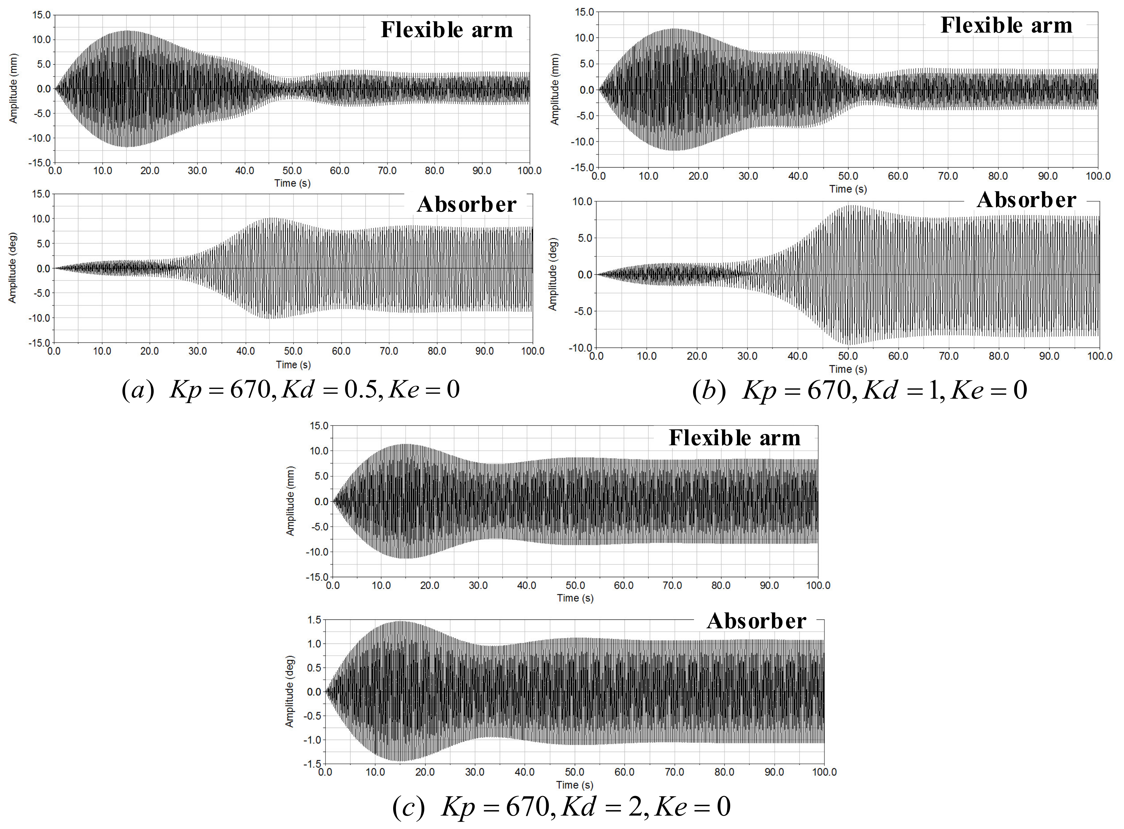
Figure 12 shows the effect of the speed feedback gain coefficient $Kd$ on the saturation control performance of the flexible manipulator. From Figure 12a,b, it can be seen that the saturation has been successfully established and the primary resonance response of the flexible manipulator has been effectively suppressed. In Figure 12c, however, excessive $Kd$ leads to a failure in the establishment of the saturation. Therefore, a smaller speed feedback gain coefficient $Kd$ can better decrease the saturation amplitude.

Figure 13 shows the effect of coupling gain coefficient $Ke$ on the saturation control performance of the flexible manipulator. From Figure 13a,b, it can be seen that a larger coupling gain coefficient $Ke$ can better decrease the saturation amplitude. Through comparing Figure 12c and Figure 13c, it is found that the system can change from the unsaturated state to the saturated state by introducing the coupling gain coefficient $Ke$.

Finally, a comparison of the primary resonance amplitudes of the flexible manipulator with and without the vibration absorber is shown in Figure 14. If the vibration absorber is not equipped, the primary resonance amplitude is approximately 18.51 mm. If the vibration absorber is working, however, the primary resonance amplitude decreases to 10.6 mm at 10.1 s, 3.02 mm at 33 s, and 1.60 mm at 52 s. Approximately 90% of the primary resonance amplitude has been suppressed from 52 s to 100 s. These results have verified the effectiveness of the suggested primary resonance control method based on the saturation.

9. Experimental Study

In the theoretical study, Section 6 revealed the saturation principle, and Section 7 showed the vibration absorber configuration method to optimize saturation control. Therefore, in the experimental study of this section, the primary resonance experiment of the flexible manipulator will be first implemented to verify whether the primary resonance occurs. Next, the effectiveness of saturation control method will be validated under the condition of primary resonance. Finally, the correctness of the vibration absorber configuration method will be verified by choosing different $k_d$ and $e_1$.

9.1. Setup

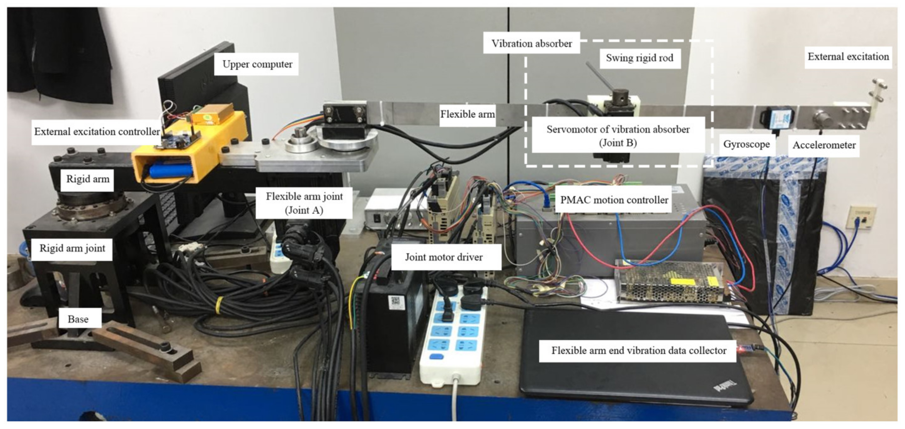
The experimental setup is designed as shown in Figure 15. The dimensions and saturation control schemes of the experimental model are identical to the theoretical and virtual prototype models. The rigid arm is hinged on the base through the joints, and its cantilever end is jointed with the flexible arm to form a 2-DOF manipulator. Through material selection and size design, the deformation of the flexible arm only occurs in the horizontal direction. The vibration absorber installed on the flexible arm is composed of a swing rod and a servomotor. The PMAC (programmable multi-axes controller) motion controller receives the feedback signal from the encoder and synchronously controls joint B. The external excitation controller controls the motor at the end of the flexible arm to generate an external excitation used to excite the primary resonance of the flexible arm. The accelerometer measures the real-time acceleration at the end of the flexible arm, which is processed by the adapter and fed back to the PMAC motion controller as the control signal. The gyroscope attached to the end of the flexible arm collects the motion data and transmits the signal to the upper computer through the TTL-USB module. The upper computer signal and absorber motor encoder signal are compared to ensure the consistency of experimental results.

9.2. Primary Resonance Experiment

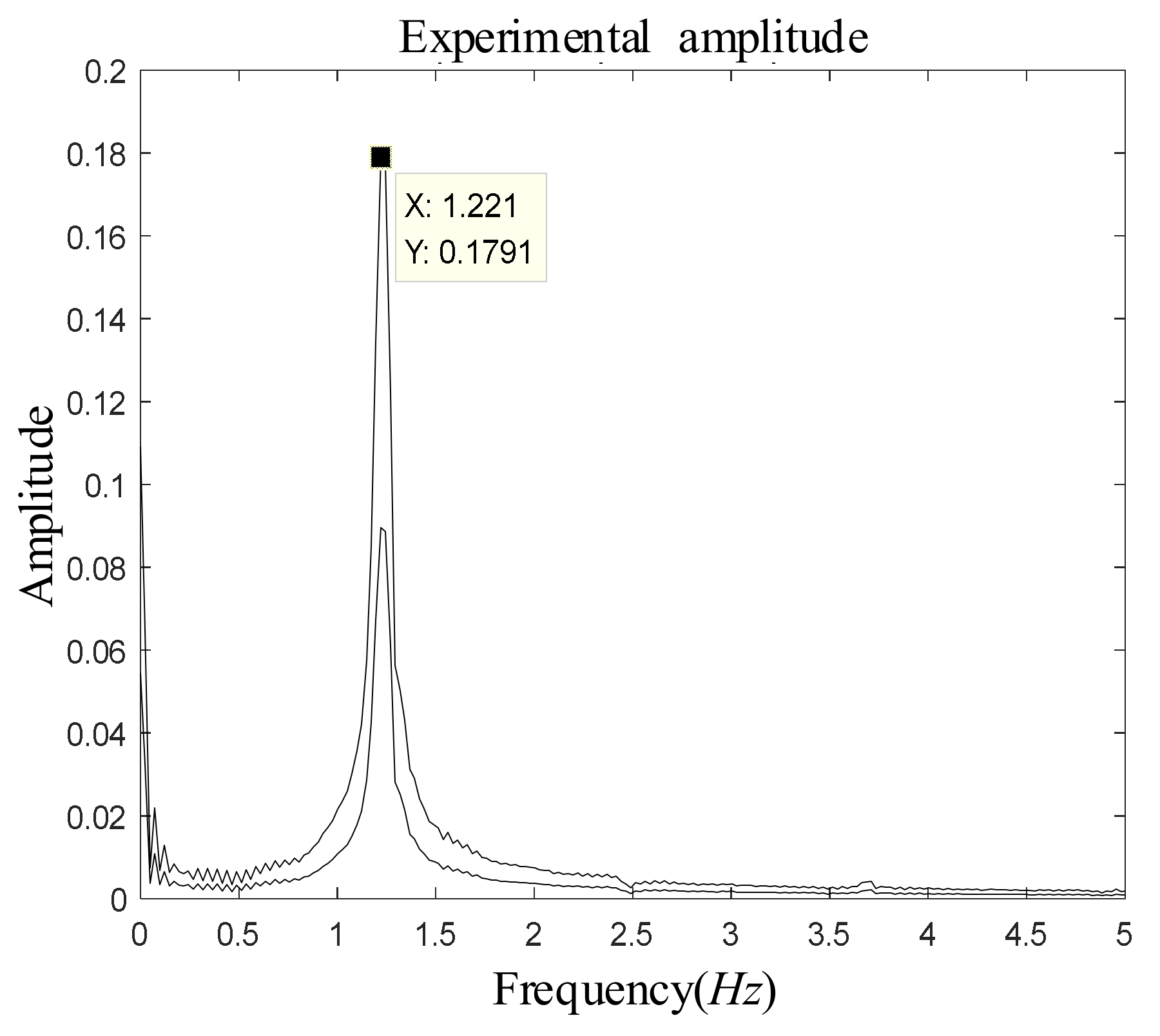
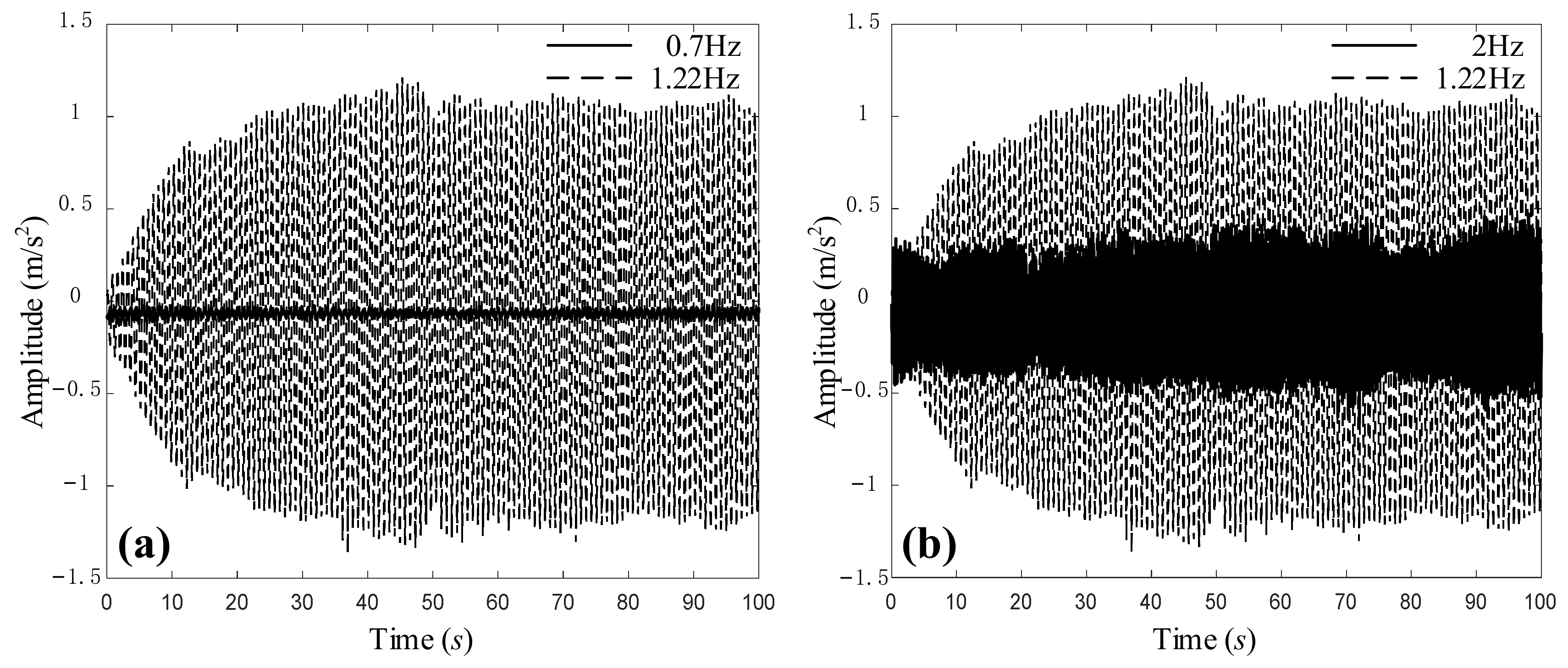
The successful establishment of the primary resonance is a prerequisite for conducting saturation experiments. In this section, the establishment of the primary resonance is verified by comparing the end amplitude of the flexible arm under different external excitations. As shown in Figure 16, the natural frequency of the flexible arm with the vibration absorber is $1.22 \mathrm{Hz}$. Therefore, the external excitation frequencies are selected as $0.70\mathrm{Hz}$, $1.22 \mathrm{Hz}$, and $2.00 \mathrm{Hz}$. All of their amplitudes are $0.5 \mathrm{N}$. The rotational speeds of two arm joints are ${\dot{\theta }}_1=0.01$ rad/s and ${\dot{\theta }}_2=0.01$ rad/s, respectively.

In Figure 17, the solid line indicates the end amplitude of the flexible arm at external excitation frequencies of $0.700 \mathrm{Hz}$ and $2.00 \mathrm{Hz}$, respectively; and the dotted line indicates the end amplitude of the flexible arm at external excitation frequencies of $1.22 \mathrm{Hz}$. Because the external excitation frequency of $1.22 \mathrm{Hz}$ is close to the natural frequency of the flexible arm with the vibration absorber, primary resonance occurs. However, as the other two external excitation frequencies are far from the natural frequency of $1.22 \mathrm{Hz}$, they cannot excite large amplitude. This phenomenon demonstrates that the primary resonance may arise when the external excitation frequency is close to the natural frequency of the flexible arm with the vibration absorber.

9.3. Saturation Control Experiment

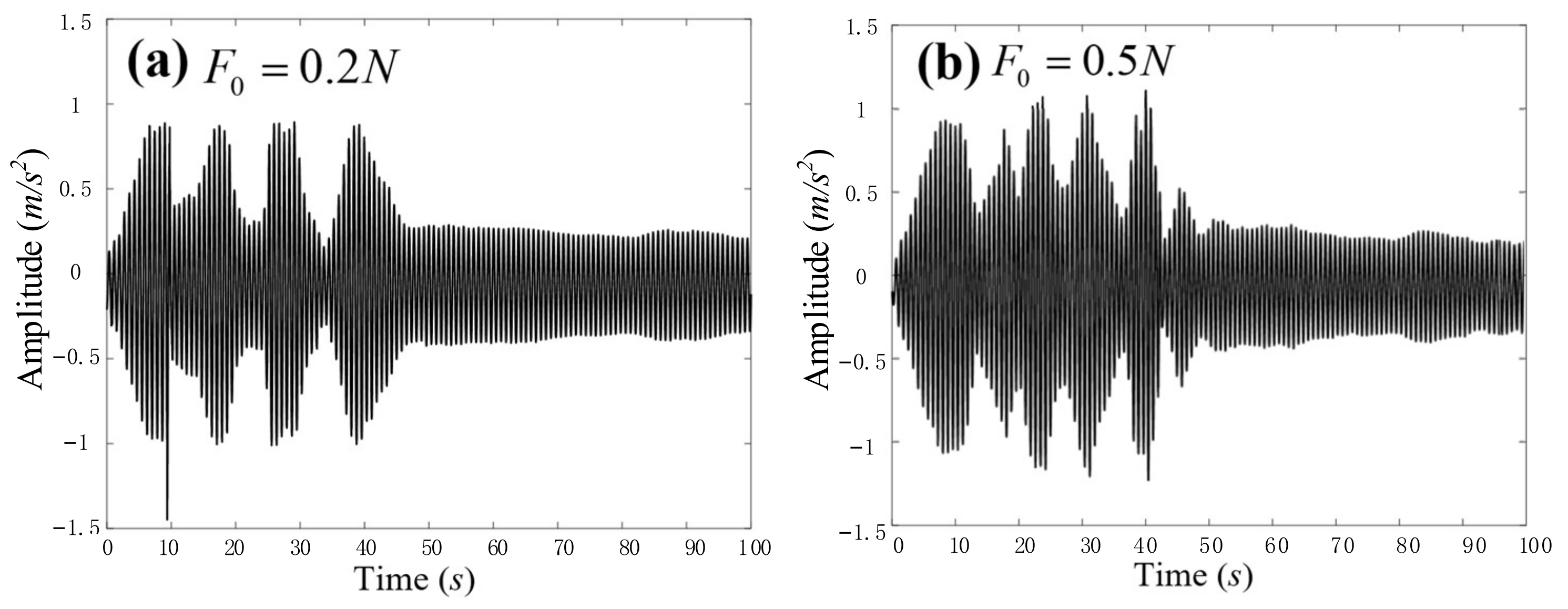
Section 5 and Section 6 revealed the saturation principle and analyzed the effectiveness of the saturation control. According to the theoretical analysis in Section 5 and Section 6, the experiments on the effectiveness of saturation control method are implemented by applying external excitations with different amplitudes to the end of the flexible arm. To ensure 1:2 internal resonance, the position feedback gain coefficient $k_p=0.061\left(\mathrm{Nmm}/cts\right)$. The speed feedback gain coefficient and the coupling feedback gain coefficient are $k_d=0.002$ and $e_1=0$, respectively. Figure 18a,b shows the amplitude of the flexible arm subjected to the external excitation amplitude of $0.2 \mathrm{N}$ and $0.5 \mathrm{N}$, respectively. Despite the change in external excitation amplitude, the steady-state saturation amplitude of the flexible arm remains around $0.3 \mathrm{m}/s^2$. The experiment results have verified the theoretical conclusion that the saturation amplitude is not affected by the external excitation amplitude.

9.4. Configuration Experiment of Saturation Absorber

According to the analysis in Section 7, the configuration experiments of saturation absorber is implemented.

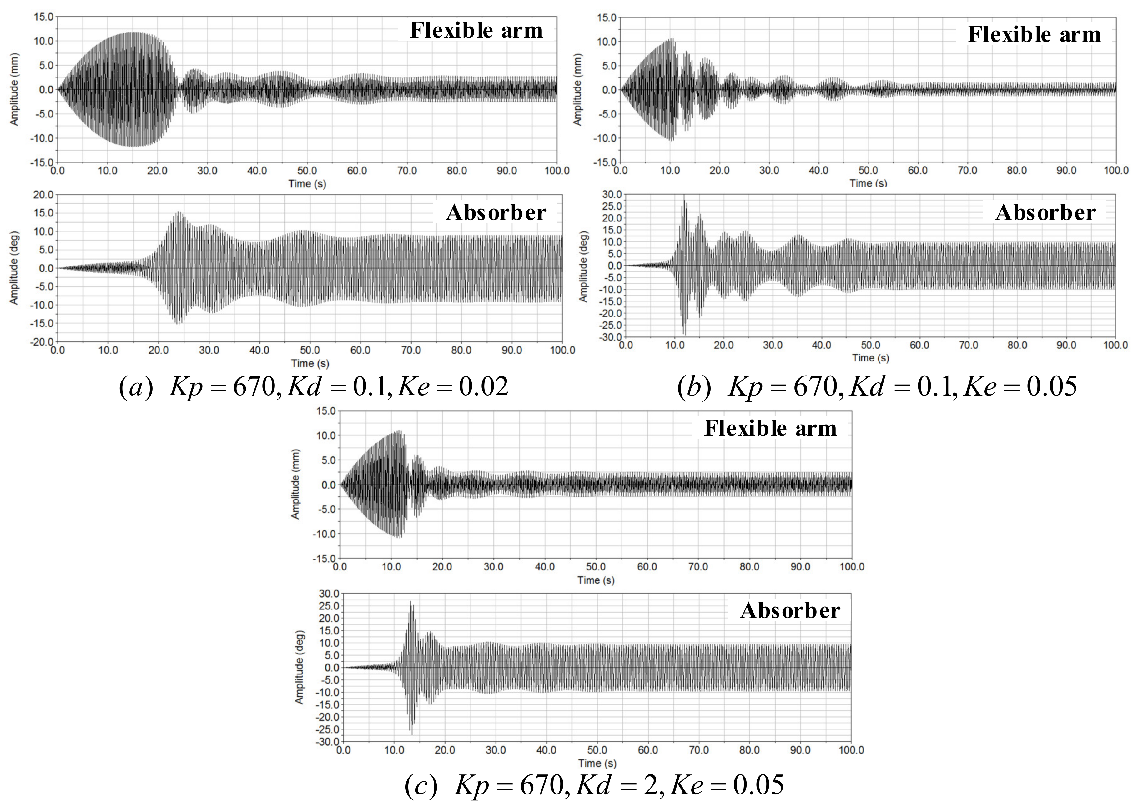
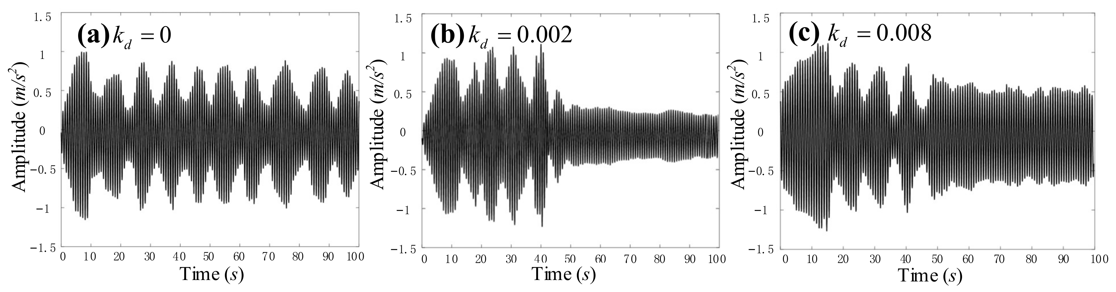
First, the effect of the speed feedback gain coefficient $k_d$ on saturation control performance is investigated. The coupling gain coefficient $e_1$ is set to 0, and the speed feedback gain coefficient $k_d$ is, respectively, set to 0, 0.002, and 0.008. As shown in Figure 19a, when $k_d=0$, the flexible arm cannot reach the saturation state. When $k_d=0.002$ or $k_d=0.008$, however, saturation can be successfully established. Through comparing Figure 19b,c, it is found that the saturation amplitude of the flexible arm is smaller when $k_d=0.002$. It is proven that reducing $k_d$ in a certain range can decrease the saturation amplitude. This phenomenon agrees with the theoretical and simulation results.

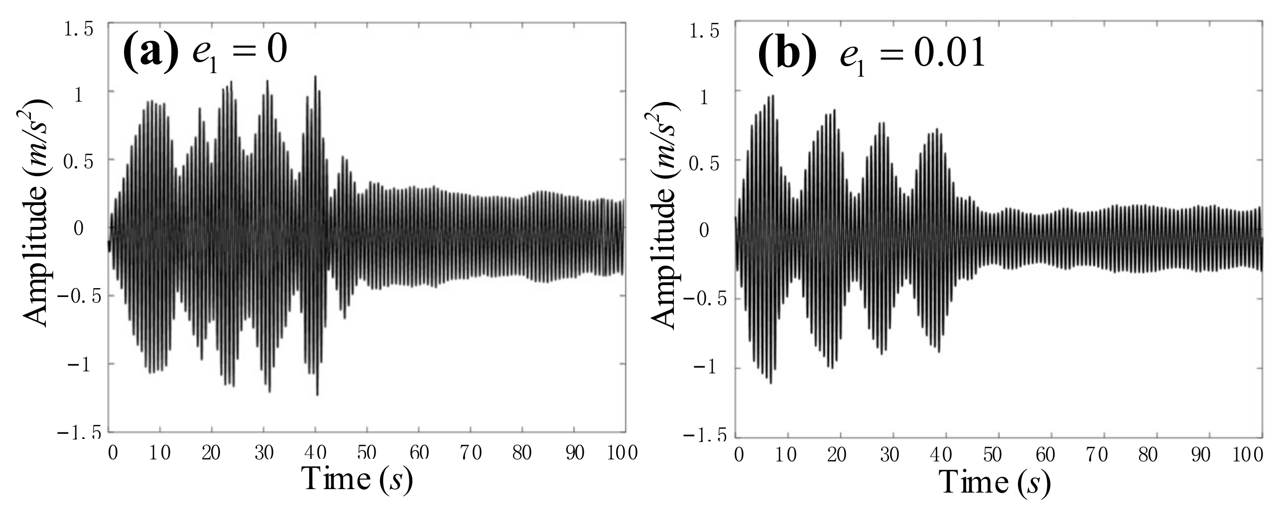
Second, the effect of different coupling gain coefficients $e_1$ on saturation control performance is investigated under the speed feedback gain coefficient $k_d=0.002$. Through comparing Figure 20a,b, it can be clearly observed that, if $e_1$ increases from 0 to 0.01, the time used to establish the saturation decreases from 50 s to 45 s, and the saturation amplitude of the flexible arm decreases as well. This phenomenon has verified our idea that introducing modal coupling can improve saturation control performance.

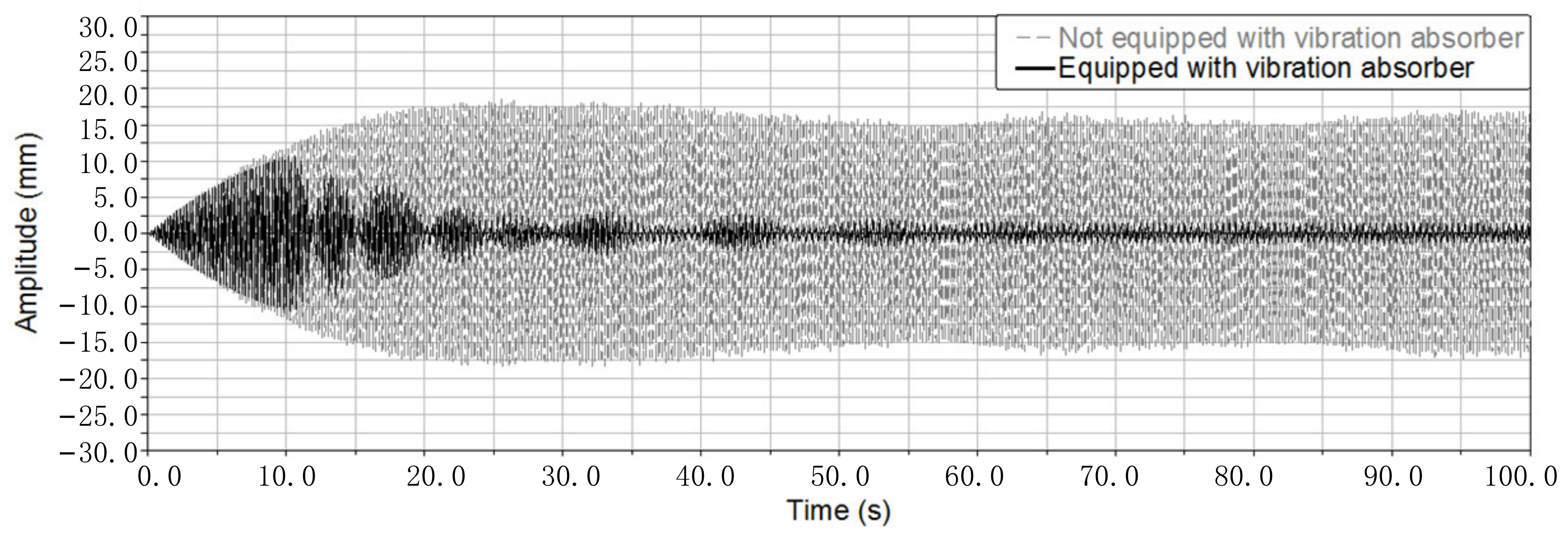
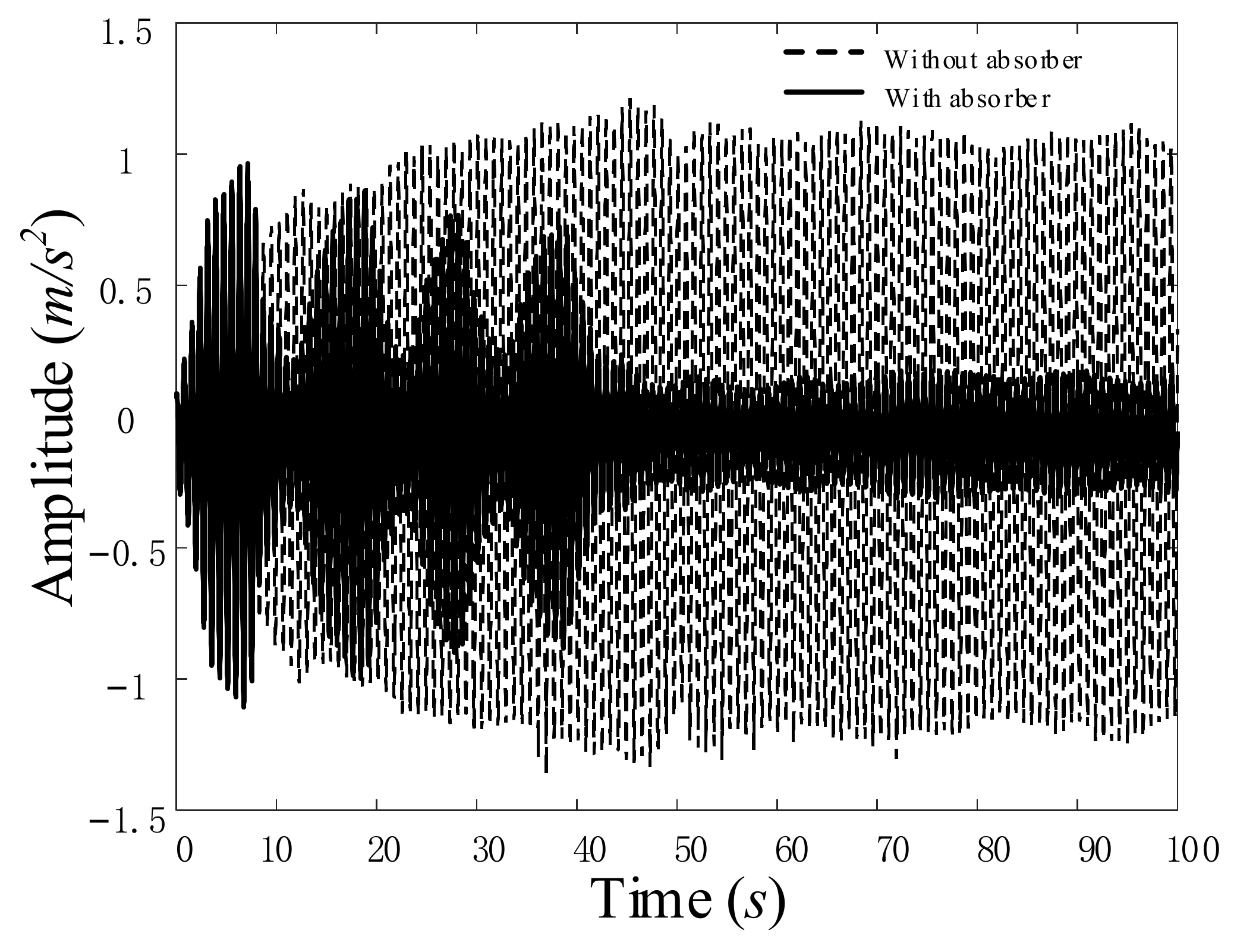
Finally, in order to compare the effect of saturation control, Figure 21 shows the primary resonance amplitude of the flexible arm with and without the vibration absorber. It can be seen that the maximal amplitude of vibration response of the flexible arm without the vibration absorber fluctuates at 1.2 m/s², whereas the maximal amplitude of vibration response of the flexible arm with the vibration absorber fluctuates at 0.2 m/s². This result has demonstrated that the primary resonance amplitude of the flexible arm has been effectively reduced by 83% with the help of the saturation.

10. Discussion

Because the theoretical analysis method, the virtual prototyping simulation method, and the experimental method are implemented in different ways, their research results are somewhat different. The detailed different implementation ways are as follows:

(1)

The theoretical model is derived based on the assumption mode method and Kane’s method, whereas the prototyping simulation model is established based on the finite element method.

(2)

The method of multiple scales is used to obtain the approximate analytical solutions of the nonlinear differential equations in the theoretical model. Due to the inherent limitations of the method, some assumptions, such as weak nonlinearity, small damping, and small external excitation, have to be adopted to obtain approximate analytical solutions. However, the virtual prototyping simulations and experiments have no such limitations.

(3)

In the theoretical study, the position feedback gain coefficient $k_p$, the speed feedback gain coefficient $k_d$, and the coupling gain coefficient $e_1$ are implemented by the theoretical formulae. However, these parameters are implemented by the MATLAB/Simulink software in the prototyping simulation model and implemented by the feedback control algorithm of the PMAC motion controller in the experiments. Obviously, these parameters are implemented in different ways and thus cannot be exactly the same in quantity.

(4)

In the theoretical study and the virtual prototyping simulations, the vibration responses are represented in displacement. However, the displacement is difficult to measure accurately in the experimental study. Thus, the vibration responses of the flexible manipulator are measured by the accelerometer in the experiments and represented in acceleration.

Despite the above differences, these research results have qualitatively verified that the primary resonance of the flexible manipulator can be effectively suppressed by the suggested saturation-based method, and the saturation control performance can be significantly improved by adjusting the control parameters of the suggested vibration absorber.

11. Conclusions

In this paper, a new nonlinear saturation-based control method is put forward to suppress the primary resonance of a flexible manipulator. A vibration absorber with variable stiffness/damping is designed to establish an energy exchange channel based on 1:2 internal resonance for the saturation. A novel idea of modal coupling enhancement is proposed, and a nonlinear coupling term is constructed and introduced into the control torque for improving saturation performance by strengthening the coupling relationship between the mode of the vibration absorber and the controlled mode of the flexible manipulator. Through stability analysis on the primary resonance response, the saturation mechanism is successfully established, and the effectiveness of the saturation control algorithm is validated. Three important indexes are extracted and used to optimize saturation control, including the saturation amplitude, the external excitation threshold, and the saturation control bandwidth. The virtual prototyping simulations and the experiment results are promising and have verified the feasibility of the suggested saturation-based method for suppressing the primary resonance of the flexible manipulator.

References

- Liu, H.B.; Geng, D.X.; Li, J.Y. Kinematics analysis and experimental study on three-dimensional space bending flexible pneumatic arm. Adv. Mech. Eng. 2020, 12, 1–16. [Google Scholar]
- Chu, M.; Chen, G.; Jia, Q.X. Simultaneous positioning and non-minimum phase vibration suppression of slewing flexible-link manipulator using only joint actuator. J. Vib. Control 2014, 20, 1488–1497. [Google Scholar] [CrossRef]
- Subedi, D.; Tyapin, I.; Hovland, G. Review on modeling and control of flexible link manipulators. Modeling Identif. Control 2020, 41, 141–163. [Google Scholar] [CrossRef]
- Alandoli, E.A.; Lee, T.S. A critical review of control techniques for flexible and rigid link manipulators. Robotica 2020, 38, 2239–2265. [Google Scholar] [CrossRef]
- Zhang, X.; Yu, H.; He, Z.; Huang, G.; Chen, Y.; Wang, G. A metamaterial beam with inverse nonlinearity for broadband micro-vibration attenuation. Mech. Syst. Signal Process. 2021, 159, 107826. [Google Scholar] [CrossRef]
- Nayfeh, A.H.; Mook, D. Nonlinear Oscillations; Wiley: New York, NY, USA, 1979. [Google Scholar]
- Silva, C.J.; Daqaq, M.F. Nonlinear flexural response of a slender cantilever beam of constant thickness and linearly-varying width to a primary resonance excitation. J. Sound Vib. 2017, 389, 438–453. [Google Scholar] [CrossRef]
- Mokhtari, A.; Jalili, M.M.; Mazidi, A. Study on frequency response and bifurcation analyses under primary resonance conditions of micro-milling operations. Appl. Math. Model. 2020, 87, 404–429. [Google Scholar] [CrossRef]
- Gao, P.; Hou, L.; Chen, Y. Analytical analysis for the nonlinear phenomena of a dual-rotor system at the case of primary resonances. J. Vib. Eng. Technol. 2021, 9, 529–540. [Google Scholar] [CrossRef]
- Kumar, P.; Pratiher, B. Influences of generic payload and constraint force on modal analysis and dynamic responses of flexible manipulator. Mech. Based Des. Struct. Mach. 2020, 1–19. [Google Scholar] [CrossRef]
- Ding, H.; Huang, L.; Mao, X.; Chen, L. Primary resonance of traveling viscoelastic beam under internal resonance. Appl. Math. Mech. 2017, 38, 1–14. [Google Scholar] [CrossRef] [Green Version]
- Lajimi, S.A.M.; Heppler, G.R.; Abdel-Rahman, E.M. Primary resonance of a beam-rigid body microgyroscope. Int. J. Non-Linear Mech. 2015, 77, 364–375. [Google Scholar] [CrossRef]
- Li, F.M.; Yao, G.; Zhang, Y. Active control of nonlinear forced vibration in a flexible beam using piezoelectric material. Mech. Adv. Mater. Struct. 2016, 23, 311–317. [Google Scholar] [CrossRef]
- Bab, S.; Khadem, S.E.; Abbasi, A.; Shahgholi, M. Dynamic stability and nonlinear vibration analysis of a rotor system with flexible/rigid blades. Mech. Mach. Theory 2016, 105, 633–653. [Google Scholar] [CrossRef]
- Zhang, G.C.; Chen, L.Q.; Li, C.P.; Ding, H. Primary resonance of coupled cantilevers subjected to magnetic interaction. Meccanica 2017, 52, 807–823. [Google Scholar] [CrossRef]
- Li, Y.Q.; Zhou, M.; Wang, T. Nonlinear primary resonance with internal resonances of the symmetric rectangular honeycomb sandwich panels with simply supported along all four edges. Thin-Walled Struct. 2020, 147, 106480. [Google Scholar] [CrossRef]
- Yektanezhad, A.; Hosseini, S.A.; Tourajizadeh, H.; Zamanian, M. Vibration analysis of flexible shafts with active magnetic bearings. Iran. J. Sci. Technol. Trans. Mech. Eng. 2020, 44, 403–414. [Google Scholar] [CrossRef]
- Gu, X.J.; Zhang, W.; Zhang, Y.F. Nonlinear vibrations of rotating pretwisted composite blade reinforced by functionally graded graphene platelets under combined aerodynamic load and airflow in tip clearance. Nonlinear Dyn. 2021, 105, 1503–1532. [Google Scholar] [CrossRef]
- Arena, A.; Lacarbonara, W. Piezoelectrically induced nonlinear resonances for dynamic morphing of lightweight panels. J. Sound Vib. 2021, 498, 115951. [Google Scholar] [CrossRef]
- Nayfeh, A.H.; Mook, D.T.; Marshall, L.R. Nonlinear coupling of pitch and roll modes in ship motions. J. Hydronautics 1973, 7, 145–152. [Google Scholar] [CrossRef]
- Haddow, A.G.; Barr, A.D.; Mook, D.T. Theoretical and experimental study of modal interaction in a two-degree-of-freedom structure. J. Sound Vib. 1984, 97, 451–473. [Google Scholar] [CrossRef]
- Oueini, S.S.; Nayfeh, A.H.; Golnaraghi, M.F. A theoretical and experimental implementation of a control method based on saturation. Nonlinear Dyn. 1997, 13, 189–202. [Google Scholar] [CrossRef]
- Pai, P.F.; Wen, B.; Naser, A.S.; Schulz, M.J. Structural vibration control using pzt patches and non-linear phenomena. J. Sound Vib. 1998, 215, 273–296. [Google Scholar] [CrossRef]
- Saguranrum, S.; Kunz, D.L.; Omar, H.M. Numerical simulations of cantilever beam response with saturation control and full modal coupling. Comput. Struct. 2003, 81, 1499–1510. [Google Scholar] [CrossRef]
- Shoeybi, M.; Ghorashi, M. Control of a nonlinear system using the saturation phenomenon. Nonlinear Dyn. 2005, 42, 113–136. [Google Scholar] [CrossRef]
- Li, J.; Li, X.; Hua, H. Active nonlinear saturation-based control for suppressing the free vibration of a self-excited plant. Commun. Nonlinear Sci. Numer. Simul. 2010, 15, 1071–1079. [Google Scholar]
- Zhao, Y.Y.; Xu, J. Using the delayed feedback control and saturation control to suppress the vibration of the dynamical system. Nonlinear Dyn. 2012, 67, 735–753. [Google Scholar] [CrossRef]
- Eftekhari, M.; Ziaei-Rad, S.; Mahzoon, M. Vibration suppression of a symmetrically cantilever composite beam using internal resonance under chordwise base excitation. Int. J. Non-Linear Mech. 2013, 48, 86–100. [Google Scholar] [CrossRef]
- Febbo, M.; Machado, S.P. Nonlinear dynamic vibration absorbers with a saturation. J. Sound Vib. 2013, 332, 1465–1483. [Google Scholar] [CrossRef]
- Chen, L.Q.; Zhang, G.C.; Ding, H. Internal resonance in forced vibration of coupled cantilevers subjected to magnetic interaction. J. Sound Vib. 2015, 354, 196–218. [Google Scholar] [CrossRef]
- Zhang, W.; Liu, G.; Siriguleng, B. Saturation phenomena and nonlinear resonances of rotating pretwisted laminated composite blade under subsonic air flow excitation. J. Sound Vib. 2020, 478, 115353. [Google Scholar] [CrossRef]
- Rocha, R.T.; Tusset, A.M.; Ribeiro, M.A. On the positioning of a piezoelectric material in the energy harvesting from a nonideally excited portal frame. J. Comput. Nonlinear Dyn. 2020, 15, 121002. [Google Scholar] [CrossRef]
- Bauomy, H.; Taha, A. Nonlinear saturation controller simulation for reducing the high vibrations of a dynamical system. Math. Biosci. Eng. 2022, 19, 3487–3508. [Google Scholar] [CrossRef]
Figure 1.
Simplified model of flexible manipulator.
Figure 2.
Primary resonance control scheme.
Figure 3.
Control model of saturation vibration absorber.
Figure 4.
Effect of external excitation on modal amplitude: (a) condition: ,; (b) condition: , , and .
Figure 5.
Saturation amplitude under different external excitation amplitudes: (a) the external excitations amplitude ; (b) the external excitations amplitude .
Figure 6.
Effect of on frequency-response curves of (a) flexible manipulator and (b) vibration absorber (when ).
Figure 7.
Figure 8.
Three indexes affected by (a) and (b) (, ).
Figure 9.
Simulation model of flexible manipulator: (a) the flexible arm model in ANSYS; (b) the flexible manipulator model with vibration absorber in ADAMS.
Figure 10.
Saturation control model in MATLAB/Simulink.
Figure 11.
FFT transform of the flexible arm terminal amplitude.
Figure 12.
Effect of on saturation amplitude of the flexible manipulator and vibration absorber.
Figure 13.
Figure 14.
Comparison of primary resonance amplitude of the flexible manipulator with and without vibration absorber.
Figure 15.
Experimental setup for primary resonance control.
Figure 16.
Frequency response curve of the flexible arm.
Figure 17.
Responses of the flexible arm under different external excitation frequencies: (a) Comparison of external excitation frequency 0.7 Hz and 1.22 Hz; (b) Comparison of external excitation frequency 2 Hz and 1.22 Hz.
Figure 18.
Effect of external excitation amplitude on primary resonance response of the flexible arm: (a) the external excitation amplitude ; (b) the external excitation amplitude .
Figure 19.
Primary resonance response of the flexible arm with different : (a) ; (b) ; (c) .
Figure 20.
Primary resonance response of the flexible arm with different : (a) ; (b) .
Figure 21.
Primary resonance response of the flexible arm with and without vibration absorber.