
A Novel Numerical Method for Theoretical Tire Model Simulation
State Key Laboratory of Automotive Simulation and Control, Jilin University, Changchun 130025, China
*
Author to whom correspondence should be addressed.
Machines 2022, 10(9), 801; https://doi.org/10.3390/machines10090801
Submission received: 17 August 2022
/
Revised: 31 August 2022
/
Accepted: 8 September 2022
/
Published: 11 September 2022
(This article belongs to the Section Vehicle Engineering)
Abstract
:Theoretical tire models are often used in tire dynamics analysis and tire design. In the past, scholars have carried out a lot of research on theoretical model modeling; however, little progress has been made on its solution. This paper focuses on the numerical solution of the theoretical model. New force and moment calculation matrix equations are constructed, and different iterative methods are compared. The results show that the modified Richardson iteration method proposed in this paper has the best convergence-stability in the steady and unsteady state calculation, which mathematically solves the problem of nonconvergence of discrete theoretical models in the published reference. A novel discrete method for solving the total deformation of tires is established based on the Euler method. The unsteady characteristics of tire models are only related to the path frequency without changing its parameters, so the unsteady state ability of the tire model can be judged based on this condition. It shows that the method in the references have significant differences at different speeds with the same path frequency under turn slip or load variations input, but the method proposed in this paper has good results.
1. Introduction
For tire and vehicle dynamics simulations and analyses, different types of tire models have been developed and categorized as empirical and theoretical models [1,2]. The empirical model, or combined theoretical and empirical model, is used for vehicle dynamics, and its model parameters are obtained by fitting measurements [2], including the MF/PAC2002 [2,3,4,5], TMeasy [6,7,8], UniTire [9,10], Hankook-Tire [11], TameTire [12,13], MF-Swift [14,15], FTire [16,17], CDTire [18,19] and RMOD-K [20,21] models, etc.
However, compared with the theoretical tire model, the empirical model is not suitable for the mechanical analysis of tire dynamics and tire design due to having too many model parameters and being dependent on experimental data. Tire design engineers should find the optimal design parameters that can satisfy the engineering requirements simultaneously and, for more efficient product development, a reliable theoretical model is essential because it enables systematic parameter study and design optimization. The theoretical models have advantages over the finite-element models in terms of computational efficiency, and they can be incorporated into the parameter study and optimization framework more easily [22]. Furthermore, combined with the static simulation data of the finite-element, using the theoretical model to achieve the steady and unsteady simulation should be a good prospect for future tire virtual development.
Fromm and Julien [3,23] proposed the brush tire model, which laid the foundation for tread modeling and tire theoretical analysis. The beam [1,3,24,25,26,27,28,29,30,31,32,33,34,35,36] and string models [3] are two classical belt/carcass modeling methods. Finally, the latest beam model includes belt tension, flexural rigidity, shear rigidity [1,22,25,26] and lateral shear force distribution [1], and the relationship between the parameters of the beam model and the design parameters of belts is established [1,22].
H. Sakai [28] pointed out that the previous practice of assuming the shape of the contact-patch as rectangular, the pressure distribution as lateral uniform and the longitudinal parabolic distribution does not reflect the reality; therefore, he studied the influence of different load, inflation pressure, camber, side slip angle and lateral force on the contact length in detail, and established a semi-empirical model of contact length with different rib along the width. Through the study of the distribution of contact patch-pressure on each rib, the empirical formula of contact patch pressure on each rib with load was established [29]. Guo Konghui established the general function of pressure distribution based on a rectangular contact patch in which the convexity, uniformity and fore-aft shift of pressure-distribution were considered [37,38,39]. Patrick Gruber, Robin S. Sharp and Andrew D studied normal and shear forces in the contact based on the finite-element model and established a 2D semi-empirical contact patch, considering longitudinal grooves as a function of vertical load and camber angle [40]. Ch. Oertel established the geometric relationship between the contact patch and vertical load, camber angle and tread profile curvature [41]; however, the contact patch length calculated by this method will be larger than the actual one, and the contact patch area caused by camber will be larger. Nakajima, Y. and Hidano, S. proposed two-dimensional contact patch considering that shear force, contact shape and contact pressure distribution are changed in the fore–aft and lateral direction caused by the camber, fore–aft and lateral external force [1,42], and the deficiency is that the contact patch shape is simply expressed as a rectangle or trapezoid.
Analytical [3,39,43,44,45,46,47,48,49,50] and numerical methods are usually used to solve theoretical models. The advantage of the former is high efficiency, but it is only suitable for simple theoretical models. With the increase of the complexity of the theoretical model, the numerical method becomes more and more important. TreadSim [3] is a typical representative for the steady-state numerical solution; however, the iteration process turned out to be unstable for certain combinations of vertical load, belt yaw and belt bend stiffness [51], and the method proposed in [51] does not actually solve the problem essentially by iteration. For unsteady-state numerical solutions, there are two different (but essentially the same) methods that are both based on the Lagrange description. An element that leaves the contact patch at one side is redefined in the model so that it will enter the contact patch at the opposite side. After a new element has entered the contact patch, the elements are also renumbered so that element number one is always the first element in the contact patch, and when the traveling distance in an increment time is larger than the distance between adjacent tread elements, a linear-interpolation method is used [52,53,54,55]. However, this method has some problems under the condition of turn slip or load variations inputs, which will be discussed in this paper. There are many methods for the iterative solution of matrix equations, including the traditional [56,57] and the latest [58,59], and different methods are suited for different application scenarios. For dynamic equations of tire models which usually consider mass, Newton’s method and the Newmark-beta method are always used [60,61]. However, in this paper, we do not intend to focus on the development of new iterative methods, but to reconstruct the matrix equations that can meet the application requirements of different iterative methods and compare several common iterative methods to select the most suitable for the discrete theoretical model and make appropriate optimizations.
In this paper, a novel matrix equation for the force and moment calculation is constructed and different iterative methods are compared under steady-state constant side slip angle and unsteady-state conditions, including the step side slip, sine side slip, load variations at constant side slip, sine side slip angle at constant turn slip and sine longitudinal slip at constant side slip inputs. It shows that only the modified Richardson method proposed in this paper can complete all of the simulations without any convergence. A novel, discrete solution method for tire total deformation is proposed based on the Euler method, and time derivatives are replaced by spatial gradients. Furthermore, based on the condition of the unsteady characteristics of tire models only relating to the path frequency without changing their parameters, the discrete solution method proposed is compared with reference [52,53,54,55] under different unsteady-state conditions, including the step side slip angle, sine side slip angle, load variations at constant side slip angle, step turn slip simulation, sine longitudinal combined with a constant side slip, sine turn combined with a constant side slip and load variations at constant longitudinal and side slip inputs. It shows that the simulation results have little difference by using the proposed method, but the reference method has a significant difference under turn slip or load variations inputs at different speed or, more precisely, the ratio between the distance of the contact patch center traveling in space within the time interval and distance between adjacent tread elements in the contact patch. However, this paper only studies the numerical solution method of the theoretical model in detail, and the results of the comparison between the model and the experiment show that a refined contact patch model considering camber and the influence of lateral force and longitudinal force on the contact patch model demonstrate the need for more in-depth research on the dynamic friction model, considering that the influences of contact pressure and slip velocity are added to the theoretical model.
The sections of this paper are arranged as follows. In Section 2, the tire total deformation discrete solution method based on the Euler method will be given. In Section 3, the modeling method of belt/carcass deformation, contact patch, stress direction in the sliding region and anisotropic of tread stiffness is described. In Section 4, according to the adhesion and sliding region, the matrix equations for the calculation of force and torque are established, and the advantages and disadvantages of different iterative methods are compared. In Section 5, the theoretical model is compared with the experiment to verify the rationality of the theoretical model parameters, and based on the principle that the unsteady state only depends on the path frequency, the discrete solution method proposed in this paper is compared with reference [52,53] unsteady-state conditions. Finally, the discussion and conclusions will be given in Section 6.
2. Tire Total Deformation Discrete Solution Method Based on the Euler Method
The total deformation of tires caused by friction consists of tread and carcass. When the tire deformation is described, two coordinate systems are used; one is the road coordinate system and the other is the contact patch coordinate system , named as . When the tire slips relative to the road surface, the friction forces makes the tire deform relative to the contact patch coordinates , as shown in Figure 1. is the contact point at undeformed state and is the vector of relative to the system. represents the contact patch center and is the vector relative to the system. represents the contact point vector at undeformed state, represents the total tire deformation vector and is the vector of relative to . represents the sideslip angle and represents the yaw angle of the -axis with respect to the -axis.
The position of the tread location relative to can be expressed as the equation:
Herein, . So, there is the slip velocity of the tread relative to the road:
where is the contact patch center velocity and and are the base vector. When there is no relative slip between the tread and the road surface, , then
Herein, , , , expression of Equations (3) and (4) by the Euler method
Then, there are:
Herein, , , , , and is practical slip, is side slip angle, is the longitudinal theoretical slip, is the lateral theoretical slip and is the turn theoretical slip. Equations (7) and (8) are only related to the coordinates of the contact patch and the space position of the contact patch center. The expression of Equations (7) and (8) in a discrete method:
According to Equations (9) and (10), there are tire total deformation:
Herein:
represents the distance between adjacent tread elements in the contact patch.
represents the distance of the contact patch center traveling in space within the time interval .
If is set to zero, it can be transformed into a steady state.
3. Model Description
3.1. Belt/Carcass Deformation [23,54]
Assuming that longitudinal translation deformation only occurs under longitudinal force [54]:
where is the longitudinal translational stiffness of carcass. Under lateral force, the carcass is expressed as the deformation of an infinite beam under concentrated force. The beam has in-plane flexural rigidity , where is the moment of the inertia of the area, is the Young’s modulus of the belt in the circumferential direction, is the lateral fundamental spring rate per unit length in the circumferential direction and the tension is uniformly distributed in the belt width direction [23]. represents bending moment and represents shear force, as shown in Figure 2. The left diagram shows the equilibrium of forces of the beam section and the right diagram shows model of the beam on the elastic foundation.
The equilibrium of forces acting on the element of length along the belt width results in the following equation:
Furthermore, according to (14)–(16), the differential equation of the lateral deformation of the beam can finally be expressed as:
According to boundary conditions, (1) ; (2) ; and (3) , there is:
Herein:
Torsional deformation of carcass under aligning moment [54].
is the carcass torsion stiffness.
Therefore, the lateral deformation of the carcass under lateral force and an aligning moment can be expressed as
3.2. Contact Patch
Reference [41] presents a method for calculating the shape of a contact patch based on vertical force. Due to the fact that this method usually leads to a large contact patch area following camber input, this paper does not consider camber.
where is free radius, is the loaded radius, is the vertical deflection, is the lateral radius and is the lateral direction curvature exponent.
However, directly according to this method, the obtained contact length will be larger. A correction method is proposed as follows:
Then, the contact patch can be obtained when .
The pressure distribution of ground imprinting is expressed as follows [41,54]:
assuming that is a constant, which can be obtained according to .
is the contact length at position , is the contact width at position and is the convexity factor along the contact width.
where is convexity factor of contact pressure along contact length, is the contact pressure center-offset factor and is the contact pressure-uniformity factor.
When considering the tread pattern longitudinal groove, the of the corresponding position is set to zero. The contact patch example is shown as in Figure 3.
3.3. Direction of Stress in the Sliding Regions
As shown in Figure 4, are the upper (which is attached to the belt) and lower end of the bristle and the bristle deformation, respectively, at previous times. correspond to the current time. is the bristle slip displacement vector relative to the road.
then
For sliding regions, the sliding direction determines the direction of deformation, so the vector is in the same direction as and is on vector ; that is to say determines the direction of .
3.4. Stiffness of the Tread Element
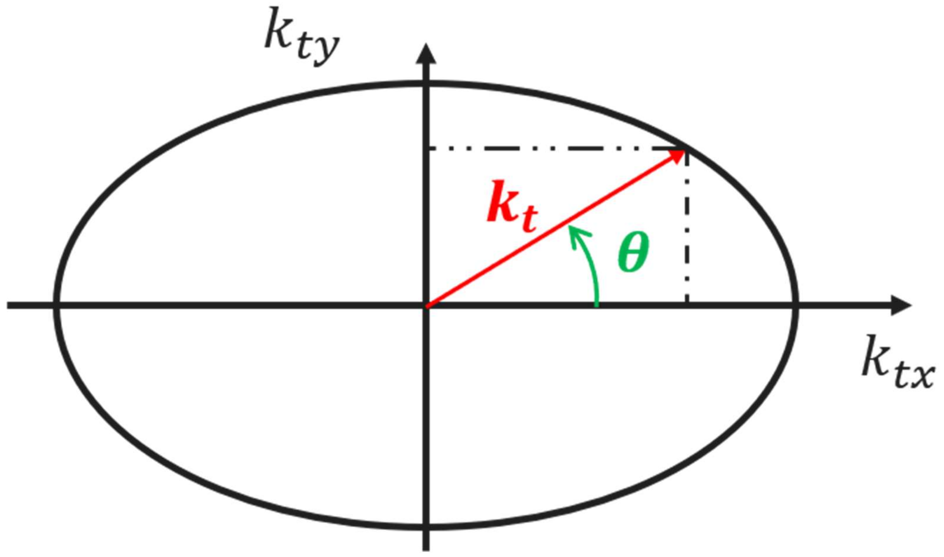
The pattern block structure usually leads to the anisotropy of tread element stiffness. It is assumed that the stiffness satisfies the elliptic equation, as shown in Figure 5:
then:
where is the deformation direction angle of the tread element.
4. Iterative Method for Force and Moment Calculation
4.1. Deformation and Stress Calculation of Tread Element
When the tread element is in the adhesion region, the deformation is calculated as follows
Herein, and are obtained from Section 2, Equations (11) and (12); and are obtained from Section 3.1, Equations (13) and (17). The deformation direction angle of the tread element is expressed as
The longitudinal and lateral stresses of tread element are expressed as
If
else
Above are the stress and deformation of tread element in the sliding region.
4.2. Calculation of Force and Moment
4.2.1. Fx Calculation
4.2.2. Fy Calculation
4.2.3. Mz Calculation
According to Equations (33) and (35), there are
Make:
There are
Make:
Finally, there are
A reasonable iterative method can be constructed according to this matrix equation.
4.3. Iterative Strategy
4.3.1. Matrix Splitting Method
Make:
then:
where , and , .
4.3.2. Steepest-Descent Method
4.3.3. Richrdson Method
4.3.4. Extrapolation Acceleration Method
According to matrixes and from Section 4.3.1, the extrapolation acceleration method can be made:
where , and are the maximum and minimum eigenvalues of , respectively.
4.3.5. Method in References [54,55]
This method obtains the solution directly from the matrix equation:
This method is equivalent to Section 4.3.1 where is equal to zero.
4.3.6. Method in References [3,51]
This method is equivalent to that of the matrix whose coefficients are equal to one, and the method is the same as in Section 4.3.1.
4.3.7. Iterative Error
If , the iterative reaches convergence, where is the iterative error tolerance.
4.3.8. Comparison of Iterative Methods
A comparison of the iterative methods at a steady state under a constant side slip angle = three deg is shown in Figure 6, and method 4 and 5’s iterative processes coincide completely.
The unsteady comparison results of different iterative methods are shown in Table 1.
Figure 6 shows that method 6 has the fastest iteration speed at a steady state, followed by method 3. It can be seen from Table 1 that although method 3 has the slowest iteration speed in unsteady state, it has the most stable convergence. As such, method 3 is selected as the iterative strategy of the discrete theoretical model. However, it should be noted that in the case of unsteady large slip, due to the fact that the coefficients of the matrix parameters tend to one but the matrix changes, the solution is sometimes not convergent, so it is necessary to improve the iterative method. Through research, it is found that the following equation can improve convergence:
The adjustment of can better improve the convergence, but it will reduce a certain convergence speed. The greater is, the better the convergence will be, but the iteration speed will be reduced, and this parameter can be reasonably selected for specific situations. This paper recomments , and the simulation in Table 1 uses this parameter.
5. Simulation of the Discrete Theoretical Model
5.1. Model Parameters and Verification
The model parameters are listed in Table 2, Figure 7, Figure 8, Figure 9, Figure 10 and Figure 11 show the comparison between the model and the test and the test information is shown in Table 3.
The contact pressure is performed on the TekScan. The other three conditions are performed on the MTS CT Flat-trac machine (MTS System Corporation). For the sideslip angle step condition, the test procedure is to turn the steer angle first, then load and finally apply the belt speed of the MTS to 10kph within one second. It should be noted that the sign of steer angle in the table is the opposite to that of the slip angle which is determined by the MTS Flat-trac machine.
It should be noted that the response of normalized lateral force instead of lateral force with travel distance is used, which does not affect the assessment of transient behavior.
As shown in Figure 11, the aligning moment is quite different from the experimental data, and a reasonable reason is whether the local camber of the carcass caused by the lateral force is not considered, which can lead to greater aligning moment if taken into consideration.
The unsteady characteristics of tire models are only related to the path frequency without changing its parameters, so the unsteady state-ability of the tire model can be judged based on this condition and changing the ratio between the distance of the contact patch center traveling in space within the time interval and the distance between adjacent tread elements in the contact patch by changing speed. The path frequency is defined as:
where [] represents the path frequency, [] represents the time frequency and [] represents the contact patch center velocity.
Next, the discrete method proposed for tire total-deformation calculation in this paper (Section 2) will be compared with the references [52,53], and the comparison results of two methods are given. The comparison error calculation method is as follows:
where represents the proposed method in this paper and represents the proposed method in reference [52,53].
5.2. Pure Side Slip Simulation
5.2.1. Step Side Slip Angle
The simulation results of step side slip angle with the proposed method and the reference method are as shown in Figure 12.
5.2.2. Sine Side Slip Angle
The simulation results of sine side slip angle with the proposed method and the reference method are as shown in Figure 13.
5.2.3. Load Variations at Constant Side Slip Angle
The simulation results of load variations at constant side slip angle with the proposed method and the reference method are as shown in Figure 14.
5.2.4. Discussion
The above simulations have the same path frequency, and the simulation results for different speeds should also be the same, in theory. The simulation results of the proposed method are slightly different, but significant differences occur in reference methods under the load variations condition at different speeds. The simulation errors of the two methods at 3m/s are listed in Table 4.
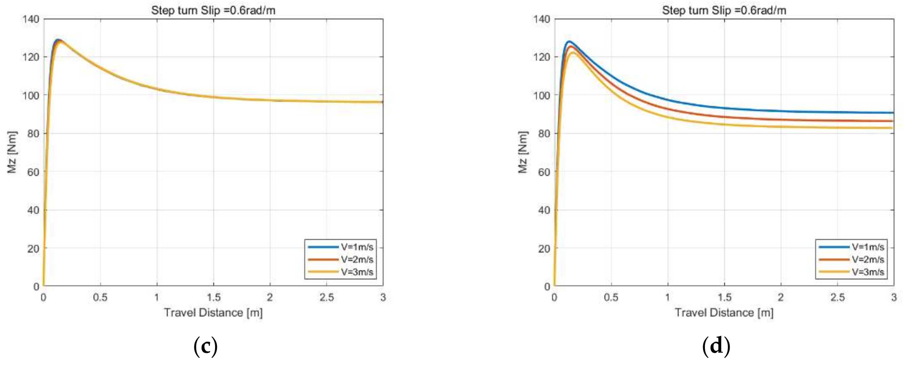
5.3. Step Turn Slip Simulation
The simulation results of step turn slip with the proposed method and the reference method are as shown in Figure 15.
The method proposed in the references is obviously not suitable for the turn slip simulation because the steady-state simulation results at different speeds are quite different. The reason is that the method proposed in the reference is based on the principle of linear interpolation in the leading edge, while the tread deformation is nonlinear during turn slip and the method fails when is much larger than . At the same time, it can be seen that the aligning moment responds quickly in the initial position, which is explained in Section 5.5.2. The simulation errors of the two methods at 3m/s are listed in Table 5.
5.4. Combined Slip Simulation
5.4.1. Sine Longitudinal Combined with a Constant Side Slip
The simulation results of sine longitudinal combined with a constant side slip with the proposed method and the reference method are as shown in Figure 16.
5.4.2. Sine Turn Combined with a Constant Side Slip
The simulation results of sine turn combined with a constant side slip with the proposed method and the reference method are as shown in Figure 17.
5.4.3. Load Variations at Constant Longitudinal and Side Slip
The simulation results of load variations at constant longitudinal and side slip with the proposed method and the reference method are as shown in Figure 18.
5.4.4. Discussion
In the case of load variations or turn slip input the reference method has obvious problems, and the conclusions are consistent with Section 5.2 and Section 5.3. The simulation errors of the two methods at 3m/s are listed in Table 6.
5.5. Deformation Analysis of Tread Element
5.5.1. Deformation of Tread Element under Step Side Slip Angle
In the side slip angle step condition, with the increase of the travel distance, the deformation of the tread element approximately changes shape from rectangular to trapezoidal and finally to triangular, as shown in Figure 19.
5.5.2. Deformation of the Tread Element under Step Turn Slip
In the turn slip step condition, the lateral deformation is first symmetrically distributed relative to the longitudinal center of contact patch, which is the reason why the slope of lateral force with the travel distance is zero at the starting position and also explains why aligning moment responds so quickly, as shown in Figure 20.
With the increase of the travel distance, the intersection point of the lateral deformation curve with the contact patch longitudinal axis gradually shifts from the center to the intersection point of the steady state. In this process, the lateral force increases continuously, and the increment gradient of the aligning moment caused by the lateral deformation decreases, which leads to a peak of the aligning moment which then decreases and finally tends to the steady state value.
At the same time, the lateral deformation is approximate to the nonlinear change of the parabolic shape, which also explains why the reference method will have problems in the turn slip input simulation.
5.5.3. Deformation of the Tread Element under Load Variations at a Constant Side Slip Angle
Figure 21 shows the that the lateral deformation of the proposed method is more regular and stable than reference. It explains why under load variations conditions at the same path frequency, when the traveling distance in an increment time is larger than the distance between adjacent tread elements, the lateral force and aligning moment of the reference method will be different.
6. Discussion and Conclusions
6.1. Discussion
Figure 7 and Figure 8 show that the contact patch parameters are reasonable, and the simulation results are consistent with the experiments. Figure 9, Figure 10 and Figure 11a show that the belt/carcass parameters are reasonable, and simulation and test results are consistent as well. However, Figure 11b shows that the aligning moment is quite different from the experimental data, and a reasonable reason is that the local camber of the carcass caused by the lateral force is not considered, which can lead to greater aligning moment if considered.
Figure 6 shows that different iterative methods converge to the same value and that the iterative method in reference [54,55] has the fastest iteration speed, followed by the modified Richardson method proposed in this paper. Table 1 shows that the modified Richardson has the best convergence and then method in reference [54,55] and the worst is the method in reference [3,51].
Figure 12, Figure 13 and Figure 16 show that whether the discrete method proposed or the references [52,53,54,55] are considered, the simulation results at different speeds with the same path frequency are only slightly different under side slip angle or longitudinal slip input. Figure 14, Figure 15, Figure 17 and Figure 18 show that for the discrete proposed method the simulation results still have slight differences, but the results of the method in the references [52,53,54,55] have significant differences at different speeds with the same path frequency, and the greater the speed difference, or more precisely the greater the ratio between the distance of the contact patch center traveling in space within the time interval and distance between adjacent tread elements in the contact patch, the greater the simulation difference. The calculation errors in Table 4, Table 5 and Table 6 also confirm the above analysis. Figure 19 shows that the tread deformation varies nearly linearly at the leading edge of the contact patch under step side slip angle, but Figure 20 shows that the tread deformation varies nonlinearly in an approximate parabolic under step turn slip. Figure 21 shows that the tread deformation is more stable by using the proposed method under the load variations input. Tread deformation explains why the methods in the reference [52,53,54,55] have problems under the turn slip or load variations inputs, since the method performs a linear interpolation process at the leading edge which is not suitable for nonlinear deformation and deformation instability. The above conclusions may be able to explain the reasons for the reference [3] “at each time step in which the wheel is rolled further over a distance equal to the interval between two successive tread elements” simulation settings.
6.2. Conclusions
In this paper, novel numerical methods for discrete theoretical tire model steady- and unsteady-state simulations are proposed. Some conclusions are as follows.
The comparison between the theoretical model and the experiment shows that the accuracy of the aligning moment needs further improvement, which may be affected by tire local carcass camber caused by lateral force, but the model parameters are reasonable.
New basic matrix equations for force and moment calculation are constructed for the convenient application of different iterative methods. Different iterative methods are studied and compared. The results show that the new modified Richardson iteration method proposed in this paper has the best convergence stability in the unsteady calculation, which mathematically solves the problem of nonconvergence of discrete theoretical models in the published references [3,51,55].
A novel discrete method for solving the total deformation of tires is established based on the Euler method. The unsteady characteristics of tire models are only related to the path frequency without changing its parameters, so the unsteady-state ability of the tire model can be judged based on this condition. It shows that the methods in the references [52,53,54,55] have significant differences at different speeds with the same path frequency, and the greater the speed difference, or more precisely the greater the ratio between the distance of the contact patch center traveling in space within the time interval and distance between adjacent tread elements in the contact patch, the greater the simulation difference under the turn slip or load variations inputs. However, the method proposed in this paper has good results.
This paper only studies the numerical solution method of the theoretical model in detail. In the future, the following work needs to be carried out. The establishment of a refined contact patch model considering camber and the influence of lateral force and longitudinal force on the contact patch model and of a dynamic friction model considering the influence of contact pressure and slip velocity is added to the theoretical model. System verification of theoretical models with experiments. Furthermore, it is hoped that theoretical models can be used in tire virtual development, since the computational efficiency of the finite element model is low and virtual data simulation, especially for turn slip input because the existing test machines cannot carry out this condition. Combined with the static simulation data of the finite element, using the theoretical model to achieve the steady and unsteady simulations should be a good prospect for the future of tire virtual development.
Author Contributions
Conceptualization, Q.L. and D.L.; methodology, Q.L. and D.L.; software, Q.L.; validation, Q.L., Y.M. and D.X.; formal analysis, Q.L., Y.M. and D.X.; investigation, Q.L.; resources, D.L.; data curation, Q.L., Y.M. and D.X.; writing—original draft preparation, Q.L.; writing—review and editing, D.L., Y.M. and D.X.; visualization, Q.L.; supervision, D.L.; project administration, D.L.; funding acquisition, D.L. All authors have read and agreed to the published version of the manuscript.
Funding
This research was funded by the Strategic Priority Research Program of Chinese Academy of Sciences, grant number XDC06060100.
Institutional Review Board Statement
Not applicable.
Informed Consent Statement
Not applicable.
Data Availability Statement
Not applicable.
Conflicts of Interest
The authors declare no conflict of interest.
Abbreviations
| Symbol | Description |
| Practical longitudinal slip | |
| Side slip angle | |
| Theoretical longitudinal slip | |
| Theoretical lateral slip | |
| Theoretical turn slip | |
| Distance between adjacent tread elements | |
| Distance of the contact patch center traveling in space within the time interval | |
| Longitudinal translational stiffness of carcass | |
| In-plane flexural rigidity of belt | |
| the lateral fundamental spring rate per unit length in the circumferential direction | |
| Carcass torsion stiffness | |
| Tire free radius | |
| Tire loaded radius | |
| Tire vertical deflection | |
| Tire lateral radius | |
| Lateral direction curvature exponent | |
| Contact patch shape correction quadratic coefficient | |
| Contact patch shape correction primary coefficient | |
| Convexity factor of contact pressure along contact length | |
| Contact pressure uniformity factor | |
| Contact pressure center offset factor | |
| Friction coefficient | |
| Iterative error tolerance | |
| Tread element longitudinal stiffness | |
| Tread element lateral stiffness | |
| Tread element stiffness | |
| Convexity factor of contact pressure along the contact width | |
| Iterative correction coefficient | |
| Steady-state lateral force |
References
- Nakajima, Y.; Hidano, S. Theoretical Tire Model Considering Two-Dimensional Contact Patch for Force and Moment. Tire Sci. Technol. 2022, 50, 27–60. [Google Scholar] [CrossRef]
- Kuiper, E.V.O.J.; Van Oosten, J.J.M. The PAC2002 advanced handling tire model. Veh. Syst. Dyn. 2007, 45, 153–167. [Google Scholar] [CrossRef]
- Pacejka, H.B. Tire and Vehicle Dynamics, 3rd ed.; Elsevier: Oxford, UK, 2012. [Google Scholar]
- Pacejka, H.B.; Bakker, E. The magic formula tyre model. Veh. Syst. Dyn. 1992, 21, 1–18. [Google Scholar] [CrossRef]
- Pacejka, H.B.; Besselink, I.J.M. Magic formula tyre model with transient properties. Veh. Syst. Dyn. 1997, 27, 234–249. [Google Scholar] [CrossRef]
- Hirschberg, W.; Rill, G.; Weinfurter, H. Tire model tmeasy. Veh. Syst. Dyn. 2007, 45, 101–119. [Google Scholar] [CrossRef]
- Rill, G. TMeasy—A Handling Tire Model based on a three-dimensional slip approach. In Proceedings of the XXIII International Symposium on Dynamic of Vehicles on Roads and on Tracks (IAVSD 2013), Quingdao, China, 19–23 August 2013; pp. 19–23. [Google Scholar]
- Rill, G. Road Vehicle Dynamics: Fundamentals and Modeling, 1st ed.; Taylor & Francis: Boca Raton, FL, USA, 2011. [Google Scholar]
- Guo, K.; Lu, D.; Chen, S.K.; Lin, W.C.; Lu, X.P. The UniTire model: A nonlinear and non-steady-state tyre model for vehicle dynamics simulation. Veh. Syst. Dyn. 2005, 43 (Suppl. S1), 341–358. [Google Scholar] [CrossRef]
- Guo, K.; Lu, D. UniTire: Unified tire model for vehicle dynamic simulation. Veh. Syst. Dyn. 2007, 45, 79–99. [Google Scholar] [CrossRef]
- Gim, G.; Choi, Y.; Kim, S. A semiphysical tyre model for vehicle dynamics analysis of handling and braking. Veh. Syst. Dyn. 2005, 43 (Suppl. S1), 267–280. [Google Scholar] [CrossRef]
- Février, P.; Fandard, G. Thermal and mechanical tyre modelling for handling simulation. ATZ Worldw. 2008, 110, 26–31. [Google Scholar] [CrossRef]
- Pearson, M.; Blanco-Hague, O.; Pawlowski, R. TameTire: Introduction to the model. Tire Sci. Technol. 2016, 44, 102–119. [Google Scholar] [CrossRef]
- Jansen, S.T.; Verhoeff, L.; Cremers, R.; Schmeitz, A.J.; Besselink, I.J. MF-Swift simulation study using benchmark data. Veh. Syst. Dyn. 2005, 43 (Suppl. S1), 92–101. [Google Scholar] [CrossRef]
- Schmeitz, A.J.C.; Besselink, I.J.M.; Jansen, S.T.H. Tno mf-swift. Veh. Syst. Dyn. 2007, 45, 121–137. [Google Scholar] [CrossRef]
- Gipser, M. FTire-the tire simulation model for all applications related to vehicle dynamics. Veh. Syst. Dyn. 2007, 45, 139–151. [Google Scholar] [CrossRef]
- Gipser, M. FTire and puzzling tyre physics: Teacher, not student. Veh. Syst. Dyn. 2016, 54, 448–462. [Google Scholar] [CrossRef]
- Gallrein, A.; De Cuyper, J.; Dehandschutter, W.; Bäcker, M. Parameter identification for LMS CDTire. Veh. Syst. Dyn. 2005, 43 (Suppl. S1), 444–456. [Google Scholar] [CrossRef]
- Gallrein, A.; Bäcker, M. CDTire: A tire model for comfort and durability applications. Veh. Syst. Dyn. 2007, 45, 69–77. [Google Scholar] [CrossRef]
- Oertel, C.; Fandre, A. Ride comfort simulations and steps towards life time calculations: RMOD-K tyre model and ADAMS. In Proceedings of the International ADAMS Users’ Conference, Berlin, Germany, 17–19 November 1999. [Google Scholar]
- Oertel, C.; Fandre, A. Tire model RMOD-K 7 and misuse load cases. SAE Tech. Pap. 2009. [Google Scholar] [CrossRef]
- Gil, G.; Lee, S. In-Plane Bending and Shear Deformation of Belt Contributions on Tire Cornering Stiffness Characteristics. Tire Sci. Technol. 2021, 49, 276–297. [Google Scholar] [CrossRef]
- Clark, S.K. (Ed.) Mechanics of Pneumatic Tires, 1st ed.; US Government Printing Office: Washington, DC, USA, 1971. [Google Scholar]
- Nakajima, Y. Advanced Tire Mechanics, 1st ed.; Springer: Singapore, 2019. [Google Scholar]
- Sarkisov, P. Physical Understanding of Tire Transient Handling Behavior, 1st ed.; Cuvillier Verlag: Göttingen, Germany, 2019. [Google Scholar]
- Sarkisov, P.; Prokop, G.; Kubenz, J.; Popov, S. Physical understanding of transient generation of tire lateral force and aligning torque. Tire Sci. Technol. 2019, 47, 308–333. [Google Scholar] [CrossRef]
- Sakai, H. Tire Engineering; Guranpuri-Shuppan: Tokyo, Japan, 1987. (In Japanese) [Google Scholar]
- Sakai, H. Theoretical and experimental studies on the dynamic properties of tyres Part 1: Review of theories of rubber friction. Int. J. Veh. Des. 1981, 2, 78–110. [Google Scholar]
- Sakai, H. Theoretical and experimental studies on the dynamic properties of tyres. Part 2: Experimental investigation of rubber friction and deformation of a tyre. Int. J. Veh. Des. 1981, 2, 182–226. [Google Scholar]
- Sakai, H. Theoretical and experimental studies on the dynamic properties of tyres: Part 3: Calculation of the six components of force and moment of a tyre. Int. J. Veh. Des. 1981, 2, 335–372. [Google Scholar]
- Sakai, H. Theoretical and experimental studies on the dynamic properties of tyres. Part 4: Investigations of the influences of running conditions by calculation and experiment. Int. J. Veh. Des. 1982, 3, 333–375. [Google Scholar]
- Gwanghun, G.; Parviz, E.N. An Analytical Model of Pneumatic Tyres for Vehicle Dynamic Simulations. Part 1: Pure slips. Int. J. Veh. Des. 1990, 11, 589–618. [Google Scholar]
- Gim, G.; Kim, S. A semi-physical tire model for practical cornering simulations of vehicles. In IPC-9 Paper 971283; Bali, Indonesia, November 1997. [Google Scholar]
- Gim, G.; Nikravesh, P.E. A three dimensional tire model for steady-state simulations of vehicles. SAE Trans. 1993, 102, 150–159. [Google Scholar]
- Kabe, K.; Miyashita, N. A new analytical tire model for cornering simulation. Part I: Cornering power and self-aligning torque power. Tire Sci. Technol. 2006, 34, 84–99. [Google Scholar] [CrossRef]
- Miyashita, N.; Kabe, K. A new analytical tire model for cornering simulation. Part II: Cornering force and self-aligning torque. Tire Sci. Technol. 2006, 34, 100–118. [Google Scholar] [CrossRef]
- Guo, K.H. A Unified Tire Model for Braking Driving and Steering Simulation (No. 891198); SAE Technical Paper; SAE: Warrendale, PA, USA, 1989. [Google Scholar]
- Lu, D. Modeling of Tire Cornering Properties under Transient Vertical Load and Its Effect on Vehicle Handling. Ph.D. Thesis, Jilin University, Changchun, China, 2003. [Google Scholar]
- Guo, K.; Liu, Q. A generalized theoretical model of tire cornering properties in steady state condition. SAE Trans. 1997, 106, 469–475. [Google Scholar]
- Gruber, P.; Sharp, R.S.; Crocombe, A.D. Normal and shear forces in the contact patch of a braked racing tyre. Part 1: Results from a finite-element model. Veh. Syst. Dyn. 2012, 50, 323–337. [Google Scholar] [CrossRef]
- Oertel, C. RMOD-K Formula Documentation; Brandenburg University of Applied Sciences: Brandenburg an der Havel, Germany, 2011. [Google Scholar]
- Nakajima, Y.; Hidano, S. Theoretical Tire Model for Wear Progress of Tires with Tread Pattern Considering Two-Dimensional Contact Patch. Tire Sci. Technol. 2021. [Google Scholar] [CrossRef]
- Sui, J. Study on Longitudinal and Side Slip Characteristics of Tire Under Steady State Conditions. Ph.D. Thesis, Jilin University, Changchun, China, 1995. [Google Scholar]
- Liu, Q. Analysis, Modeling and Simulation of Unsteady Sideslip Characteristics of Tire. Ph.D. Thesis, Jilin University, Changchun, China, 1996. [Google Scholar]
- Guo, K.; Liu, Q. Modelling and simulation of non-steady state cornering properties and identification of structure parameters of tyres. Veh. Syst. Dyn. 1997, 27, 80–93. [Google Scholar] [CrossRef]
- Romano, L. Advanced Brush Tyre Modelling, 1st ed.; Springer: Cham, Switzerland, 2022. [Google Scholar]
- Romano, L.; Timpone, F.; Bruzelius, F.; Jacobson, B. Analytical results in transient brush tyre models: Theory for large camber angles and classic solutions with limited friction. Meccanica 2022, 57, 165–191. [Google Scholar] [CrossRef]
- Romano, L.; Bruzelius, F.; Hjort, M.; Jacobson, B. Development and analysis of the two-regime transient tyre model for combined slip. Veh. Syst. Dyn. 2022, 1–35. [Google Scholar] [CrossRef]
- Romano, L.; Sakhnevych, A.; Strano, S.; Timpone, F. A novel brush-model with flexible carcass for transient interactions. Meccanica 2019, 54, 1663–1679. [Google Scholar] [CrossRef]
- Romano, L.; Bruzelius, F.; Jacobson, B. Unsteady-state brush theory. Veh. Syst. Dyn. 2021, 59, 1643–1671. [Google Scholar] [CrossRef]
- Hoogh, J.D. Implementing Inflation Pressure and Velocity Effects into the Magic Formula Tyre Model. Master’s Thesis, Eindhoven University of Technology, Eindhoven, The Netherlands, 2005. [Google Scholar]
- Zegelaar, P.W.A. The Dynamic Response of Tyres to Brake Torque Variations and Road Unevennesses. Ph.D. Thesis, Delft University of Technology, Delft, The Netherlands, 1998. [Google Scholar]
- Maurice, J.P. Short Wavelength and Dynamic Tyre Behaviour under Lateral and Combined Slip Conditions. Ph.D. Thesis, Delft University of Technology, Delft, The Netherlands, 2000. [Google Scholar]
- Xu, N.; Yang, Y.; Guo, K. A Discrete Tire Model for Cornering Properties Considering Rubber Friction. Automot. Innov. 2020, 3, 133–146. [Google Scholar] [CrossRef]
- Bai, F. Research on Tire Model Based on the Analysis of the Contact Patch. Ph.D. Thesis, Jilin University, Changchun, China, 2016. [Google Scholar]
- Available online: https://math.ecnu.edu.cn/~jypan/Teaching/MatrixIter/lect03_Iter_s.pdf (accessed on 1 August 2022).
- Greenbaum, A.; Chartier, T.P. Numerical Methods: Design, Analysis, and Computer Implementation of Algorithms; Princeton University Press: Princeton, NJ, USA, 2012. [Google Scholar]
- Zha, Y.; Yang, J.; Zeng, J.; Tso, C.H.M.; Zeng, W.; Shi, L. Review of numerical solution of Richardson–Richards equation for variably saturated flow in soils. Wiley Interdiscip. Rev. Water 2019, 6, e1364. [Google Scholar] [CrossRef]
- Singh, J.; Ganbari, B.; Kumar, D.; Baleanu, D. Analysis of fractional model of guava for biological pest control with memory effect. J. Adv. Res. 2021, 32, 99–108. [Google Scholar] [CrossRef]
- Yamashita, H.; Jayakumar, P.; Sugiyama, H. Physics-based flexible tire model integrated with lugre tire friction for transient braking and cornering analysis. J. Comput. Nonlinear Dyn. 2016. [Google Scholar] [CrossRef]
- Huang, S.; Wu, H.; Guo, K.; Lu, D.; Lu, L. An in-plane dynamic tire model with real-time simulation capability. Proc. Inst. Mech. Eng. Part D J. Automob. Eng. 2022. [Google Scholar] [CrossRef]
Figure 1.
Top view of tire contact area and its deformations with respect to .

Figure 2.
Model of the beam on the elastic foundation. (a) The equilibrium of forces for the beam section; (b) Belt/carcass deformation applied .
Figure 2.
Model of the beam on the elastic foundation. (a) The equilibrium of forces for the beam section; (b) Belt/carcass deformation applied .

Figure 3.
The contact patch model results.

Figure 4.
Tread element deformation and its slip displacement vector relative to the road.

Figure 5.
Tread element stiffness ellipse.

Figure 6.
Curves of lateral force and aligning moment with iteration times (a) Fy responses with iteration times; (b) Mz responses with iteration times.
Figure 6.
Curves of lateral force and aligning moment with iteration times (a) Fy responses with iteration times; (b) Mz responses with iteration times.

Figure 7.
Contact patch shape comparison between model and test.

Figure 8.
Contact pressure comparison between model and test. (a) Contact pressure along x center line; (b) Contact pressure along y center line.
Figure 8.
Contact pressure comparison between model and test. (a) Contact pressure along x center line; (b) Contact pressure along y center line.

Figure 9.
Parking comparison between model and test.

Figure 10.
Step side slip angle comparison between model and test. (a) Side slip angle = 1 deg; (b) Side slip angle = 4 deg.
Figure 10.
Step side slip angle comparison between model and test. (a) Side slip angle = 1 deg; (b) Side slip angle = 4 deg.

Figure 11.
Pure side slip comparison between model and test at 0.05 Hz at V = 10 km/h. (a) Side force Fy; (b) Aligning moment Mz.
Figure 11.
Pure side slip comparison between model and test at 0.05 Hz at V = 10 km/h. (a) Side force Fy; (b) Aligning moment Mz.

Figure 12.
Response of lateral force and aligning moment under side slip angle input. (a) Response of lateral force using the proposed method. (b) Response of lateral force using the reference method. (c) Response of aligning moment using the proposed method. (d) Response of aligning moment using the reference method.

Figure 13.
Response of lateral force and aligning moment under sine side slip angle input. (a) Response of lateral force using the proposed method. (b) Response of lateral force using the reference method. (c) Response of aligning moment using the proposed method. (d) Response of aligning moment using the reference method.


Figure 14.
Response of lateral force and aligning moment under load variations at constant side slip angle input. (a) Response of lateral force using the proposed method. (b) Response of lateral force using the reference method. (c) Response of aligning moment using the proposed method. (d) Response of aligning moment using the reference method.

Figure 15.
Response of the lateral force and aligning moment under step turn slip input. (a) Response of lateral force using the proposed method. (b) Response of lateral force using the reference method. (c) Response of aligning moment using the proposed method. (d) Response of aligning moment using the reference method.


Figure 16.
Response of lateral force and aligning moment under sine longitudinal combined with a constant side slip. (a) Response of longitudinal force using the proposed method. (b) Response of longitudinal force using the reference method. (c) Response of lateral force using the proposed method. (d) Response of lateral force using the reference method. (e) Response of aligning moment using the proposed method. (f) Response of aligning moment using the reference method.


Figure 17.
Response of lateral force and aligning moment under sine turn combined with a constant side slip. (a) Response of lateral force using the proposed method. (b) Response of lateral force using the reference method. (c) Response of aligning moment using the proposed method. (d) Response of aligning moment using the reference method.

Figure 18.
Responses of longitudinal force and lateral force aligning moments under load variations at constant longitudinal and side slip input. (a) Response of longitudinal force using the proposed method. (b) Response of longitudinal force using the reference method. (c) Response of lateral force using the proposed method. (d) Response of lateral force using the reference method. (e) Response of aligning moment using the proposed method. (f) Response of aligning moment using the reference method.

Figure 19.
Lateral deformation of the tread element at different traveling distances under the step side slip angle input. (a) Response of lateral force and aligning moment. (b) Deformation of the tread element at the contact patch center line under different travel distance. (c) Deformation of the tread element at A position. (d) Deformation of the tread element at B position. (e) Deformation of the tread element at C position. (f) Deformation of the tread element at D position. (g) Deformation of the tread element at E position. (h) Deformation of the tread element at F position.


Figure 20.
Lateral deformation of the tread element at different traveling distances under the step turn slip input. (a) Response of lateral force and aligning moment. (b) Deformation of the tread element at the contact patch center line under different travel distance. (c) Deformation of the tread element at A position. (d) Deformation of the tread element at B position. (e) Deformation of the tread element at C position. (f) Deformation of the tread element at D position. (g) Deformation of the tread element at F position. (h) Deformation of the tread element at E position.

Figure 21.
Lateral deformation of tread element at different traveling distance under load variations at a constant side slip angle. (a) Response of vertical force and lateral force for proposed method. (b) Response of vertical force and lateral force for the reference method. (c) Tread deformation at different positions for the proposed method. (d) Tread deformation at different positions for the reference method.


Table 1.
The iterative CPU times of different methods at different conditions.
| Iterative Method | Iterative CPU Time [s] and the Simulation Time Is Set to 3 s | ||||
|---|---|---|---|---|---|
| Step Side Slip | Sine Side Slip | Load Variations at Constant Side Slip | Sine Side Slip Angle at Constant Turn Slip | Sine Longitudinal Slip at Constant Side Slip | |
| Method 1 | 35.11 | 94.10 | 69.40 | no convergence | no convergence |
| Method 2 | 33.97 | 71.46 | 59.99 | no convergence | no convergence |
| Method 3 | 55.34 | 136.21 | 141.71 | 154.96 | 280.46 |
| Method 4 | 33.61 | 65.07 | 59.67 | no convergence | no convergence |
| Method 5 | 32.50 | 66.26 | 60.14 | no convergence | no convergence |
| Method 6 | no convergence | no convergence | no convergence | no convergence | no convergence |
Table 2.
The discrete tire model parameters.
| Parameters Name | Parameters Value | Parameters Name | Parameters Value |
|---|---|---|---|
| 1.3377 × 10⁸ | 4.3735 × 10⁵ | ||
| 1.0332 × 10⁸ | 1 × 10³ | ||
| 2 | 1.25 × 10⁵ | ||
| 0 | 0.2 | ||
| 0 | 1.2994 × 10⁴ | ||
| −0.05 | 1.11 | ||
| 2.01 × 10⁵ | 0.3465 | ||
| 20 | 5.4 | ||
| 3.64 | 0.145 | ||
| −0.74 | Tol | 10 | |
| 2 | 2 |
Table 3.
The test information.
| Test No. | Test Conditions | Inflation Pressure | Road Speed | Steer Angle | Steer Cycle | Vertical Load |
|---|---|---|---|---|---|---|
| 1 | Contact Pressure | 250 kPa | 0 | 0 | 0 s | 5415 N |
| 2 | Parking Maneuver | 250 kPa | 0 | 15~−15° | 32 s (Slope) | 5386 N |
| 3 | Sideslip Angle Step | 250 kPa | 0 → 10 kph | −1° | - | 5414 N |
| 250 kPa | 0 → 10 kph | −4° | - | 5407 N | ||
| 4 | Sine Sideslip Angle | 250 kPa | 10 kph | −15~15° | 20 s (0.05 Hz) | 5406 N |
Table 4.
The simulation errors at pure side slip simulation.
| Simulation Conditions | Compare Items | Error [%] |
|---|---|---|
| Step Side Slip Angle | 0.28 | |
| 1.12 | ||
| Sine Side Slip Angle | 1.37 | |
| 2.18 | ||
| Load Variations at Constant Side Slip Angle | 5.86 | |
| 7.59 |
Table 5.
The simulation errors at the step turn slip simulation.
| Simulation Conditions | Compare Items | Error [%] |
|---|---|---|
| Step Turn Slip Simulation | 141.40 | |
| 142.20 |
Table 6.
The simulation errors at combined slip simulation.
| Simulation Conditions | Compare Items | Error [%] |
|---|---|---|
| Step Turn Slip Simulation | 2.54 | |
| 1.23 | ||
| 3.67 | ||
| Sine Turn Combined with a Constant Side Slip | 61.01 | |
| 6.43 | ||
| Load Variations at Constant Longitudinal and Side Slip | 3.95 | |
| 8.49 | ||
| 8.86 |
Publisher’s Note: MDPI stays neutral with regard to jurisdictional claims in published maps and institutional affiliations. |
© 2022 by the authors. Licensee MDPI, Basel, Switzerland. This article is an open access article distributed under the terms and conditions of the Creative Commons Attribution (CC BY) license (https://creativecommons.org/licenses/by/4.0/).
Share and Cite
MDPI and ACS Style
Liu, Q.; Lu, D.; Ma, Y.; Xia, D. A Novel Numerical Method for Theoretical Tire Model Simulation. Machines 2022, 10, 801. https://doi.org/10.3390/machines10090801
AMA Style
Liu Q, Lu D, Ma Y, Xia D. A Novel Numerical Method for Theoretical Tire Model Simulation. Machines. 2022; 10(9):801. https://doi.org/10.3390/machines10090801
Chicago/Turabian StyleLiu, Qianjin, Dang Lu, Yao Ma, and Danhua Xia. 2022. "A Novel Numerical Method for Theoretical Tire Model Simulation" Machines 10, no. 9: 801. https://doi.org/10.3390/machines10090801
Note that from the first issue of 2016, this journal uses article numbers instead of page numbers. See further details here.