Inter-Stage Dynamic Performance of an Axial Compressor of a Twin-Shaft Industrial Gas Turbine †

1
School of Engineering, University of Lincoln, Lincoln LN6 7TS, UK
2
Siemens Energy Industrial Turbomachinery Ltd., Lincoln LN5 7DF, UK
*
Author to whom correspondence should be addressed.
†
This paper is an extended version of our paper published in “Cruz-Manzo, S.; Krishnababu, S.; Panov, V.; Zhang, Y. Performance calculation of a multistage axial compressor through a semi-empirical modelling framework. In Proceedings of the Global Power and Propulsion Society 2019, Beijing, China, 16–18 September 2019; Paper No. GPPS-BJ-2019-123”.
Machines 2020, 8(4), 83; https://doi.org/10.3390/machines8040083
Submission received: 10 November 2020
/
Revised: 4 December 2020
/
Accepted: 7 December 2020
/
Published: 9 December 2020
(This article belongs to the Section Automation and Control Systems)
Abstract
:In this study, the inter-stage dynamic performance of a multistage axial compressor is simulated through a semi-empirical model constructed in the Matlab Simulink environment. A semi-empirical 1-D compressor model developed in a previous study has been integrated with a 0-D twin-shaft gas turbine model developed in the Simulink environment. Inter-stage performance data generated through a high-fidelity design tool and based on throughflow analysis are considered for the development of the inter-stage modeling framework. Inter-stage performance data comprise pressure ratio at various speeds with nominal variable stator guide vane (VGV) positions and with hypothetical offsets to them with respect to the gas generator speed (GGS). Compressor discharge pressure, fuel flow demand, GGS and power turbine speed measured during the operation of a twin-shaft industrial gas turbine are considered for the dynamic model validation. The dynamic performance of the axial-compressor, simulated by the developed modeling framework, is represented on the overall compressor map and individual stage characteristic maps. The effect of extracting air through the bleed port in the engine center-casing on transient performance represented on overall compressor map and stage performance maps is also presented. In addition, the dynamic performance of the axial-compressor with an offset in VGV position is represented on the overall compressor map and individual stage characteristic maps. The study couples the fundamental principles of axial compressors and a semi-empirical modeling architecture in a complementary manner. The developed modeling framework can provide a deeper understanding of the factors that affect the dynamic performance of axial compressors.
1. Introduction
The performance of multiaxial compressors plays an important role in the operation of industrial gas turbines (IGTs). The pressure of the air entering the compressor is increased through a series of stages. Each stage comprises a set of rotor blades followed by a set of stator blades. The kinetic energy of air is increased by the rotor blades, and the stator blades transform the kinetic energy of air into static pressure. A variation of the angle of the stator blades across the different stages of an axial compressor ensures correct air diffusion at different operating conditions [1], where a simple actuator changes the angle of the variable stator guide vane (VGVs). The closure and opening of VGVs are a function of the demanded inlet guide vane (IGV) position. The IGV position is typically scheduled with respect to the gas generator speed (GGS) of gas turbines [2]. Various studies in the literature have reported multistage axial compressor models [2,3,4,5,6,7,8,9,10]. The aforementioned studies developed a model to predict the inter-stage performance of the axial-compressor at steady-state conditions. In addition, the reported models predicted the variation in the IGV and VGV in the compressor performance.
Simulink is a powerful programming environment for modeling and simulation of multidomain dynamical systems such as gas turbines. This simulation tool offers the possibility to represent governing thermodynamic equations of the IGT in the Simulink environment. Several studies have reported gas turbine models developed in the Simulink environment [11,12,13,14,15,16,17,18]. In a previous study [19], a thermodynamic model to predict the performance of a twin-shaft IGT at different operating conditions was reported. The modeling architecture considered a lumped axial compressor model and was developed using a commercial thermodynamic toolbox (Thermolib, EUtech), which is compatible with the Simulink environment. Damiani et al. [20] reported a one-dimensional stage-by-stage model to predict the design and off-design performance of a multistage axial flow compressor. The model was developed in the Matlab Simulink environment and was able to reproduce the compressor performance at different operating conditions. It was possible to predict the blade cooling system performance since the total pressure and total temperature values of the cooling air bleed offs were correctly calculated. The aforementioned studies do not consider the inter-stage dynamic performance of the axial-compressor during different engine operating conditions in the field. In a previous study [21], a 1-D semi-empirical compressor model, based on design parameters, compressor performance data set, and theoretical relations (velocity triangles for blade design) from an 11-stage axial compressor, was developed in the Matlab® environment. A high-fidelity design tool (HFDT) was used to simulate multistage axial compressor steady-state operation and assisted the development of the proposed modeling framework. HFDT is a Siemens standard streamline curvature through flow analysis [22] code that computes the aerodynamic parameters across the compressor. The model predicted the inter-stage performance of the compressor at full and part load steady-state conditions.
This manuscript is an extension from the authors’ previous study [21] and considers the integration of the 1-D compressor modeling architecture that predicts stagewise performance at steady-state conditions with the 0-D twin-shaft dynamic gas turbine model [23]. The 0-D gas turbine model, reported by Panov [23], enables the prediction of the dynamic gas turbine performance at different operating conditions. The overall modeling architecture is developed in the Simulink environment and allows inter-stage dynamic performance simulation of a multistage axial compressor during engine transient operation. In this study, the architecture of the 1-D model previously reported [21] has been extended by considering HFDT data set at different rotational speeds and with an offset in IGV position outside of its scheduled nominal position with respect to GGS. The developed 1-D compressor modeling architecture is interfaced with a 0-D twin-shaft engine model in the Simulink environment to predict the dynamic inter-stage performance of the axial compressor during a step load change, air bleed off from the engine center-casing, and offset in IGV position outside of its scheduled nominal position with respect to GGS. It is possible to simulate the dynamic performance of a multistage axial compressor during a twin-shaft IGT operation and represent it in the overall compressor map and individual stage characteristic maps. The overall modeling framework is validated with real-world test data of a twin-shaft engine measured during the load acceptance tests. The representation of the dynamic compressor performance on stage-characteristic maps can provide valuable information during the dynamic operation of an axial compressor in the field. For example, during the dynamic transition between two operating conditions, a given stage may perform close to its stability limit, which could cause instability of the whole compressor during the dynamic operation, particularly at low speeds. Such instability in the compressor could compromise the performance and operability of the whole IGT.
This manuscript is organized as follows: A brief description of the 1-D compressor modeling architecture from a previous study [21] is presented in Section 2. HFDT data set at different rotational speeds and with the offset in IGV position outside of its scheduled nominal position with respect to GGS structure are presented as well. In Section 3, a Simulink model of an IGT interfaced with the 1-D compressor model is presented. The dynamic validation of the modeling architecture with real-world data measured during load increase in an IGT is presented in Section 4. The results are presented in Section 5, which demonstrates the dynamic performance of the compressor represented in the overall compressor performance map and stage-performance maps. The manuscript is concluded with Section 6, which summarizes the main results.
2. Compressor Modeling Architecture
In a previous study [21], the 1-D model of the axial-compressor was developed. A brief summary of the devised model is described in this section. The inter-stage modeling framework considered theoretical velocity triangles, which relate the power input to the axial compressor stage. An analysis of these velocity triangles utilizing trigonometric relations and thermodynamic principles can derive the temperature and pressure rise across the compressor stages. The following equations comprise the overall modeling framework. The difference in total temperature between the outlet and inlet of the compressor stage is defined as:
where , U is the blade velocity, r is the tip radius, and ω is the angular velocity; α1,2 represents the angle of the air absolute velocity from the axial direction CX entering and leaving the rotor, , is the airflow rate, is the air density, and A is the annulus area. λ is the work-done factor and accounts for the reduction in work capacity across the compressor axial stage [1].
The pressure ratio through the stage can be defined as:
where η is the stage efficiency, and Tin is the stage inlet total temperature. The derivation of Equations (1) and (2) and the relation between the velocity triangles and thermodynamic principles have been reported by Saravanamutto et al. [24].
The 1-D inter-stage compressor model developed in the previous study [21] is mainly comprised of Equations (1) and (2) and requires the rotational speed ω, flow rate , efficiency η and ambient temperature Tamb and ambient pressure Pamb as inputs. The outputs from the 1-D compressor model are the pressure ratio PR and temperature Tout across the different stages of the axial compressor. In addition, compressor design parameters and the Equations (1) and (2) were required to develop the semi-empirical 1-D modeling architecture. The annulus area A, tip radius r and blade angles across the different stages of the compressor were provided by a compressor manufacturer. Thermodynamic parameters represented in Equations (1) and (2) such as air density , heat capacity CP, and the ratio between heat capacities γ across the different stages are calculated through data representing stagewise temperature and pressure ratio collected from an HFDT. HFDT is a Siemens standard through flow analysis code that computes the performance of the multistage compressor as an axisymmetric model. HFDT is essentially a two-dimensional computational fluid dynamics code based on the streamline curvature method, as reported by Wu [22]. For a given operating condition defined by the speed and throttle set by the compressor exit pressure, the code calculates the primary flow parameters such as pressure, the temperature at defined axial stations. Typically, these stations are located at the inlet and exit of the blade rows. The use of throughflow analysis for estimation of inter-stage pressure and temperature in a multistage axial compressor was reported in the study of Damiani et al. [20]. Schnoes et al. [25] considered throughflow analysis for the design optimization of a 15-stage axial compressor.
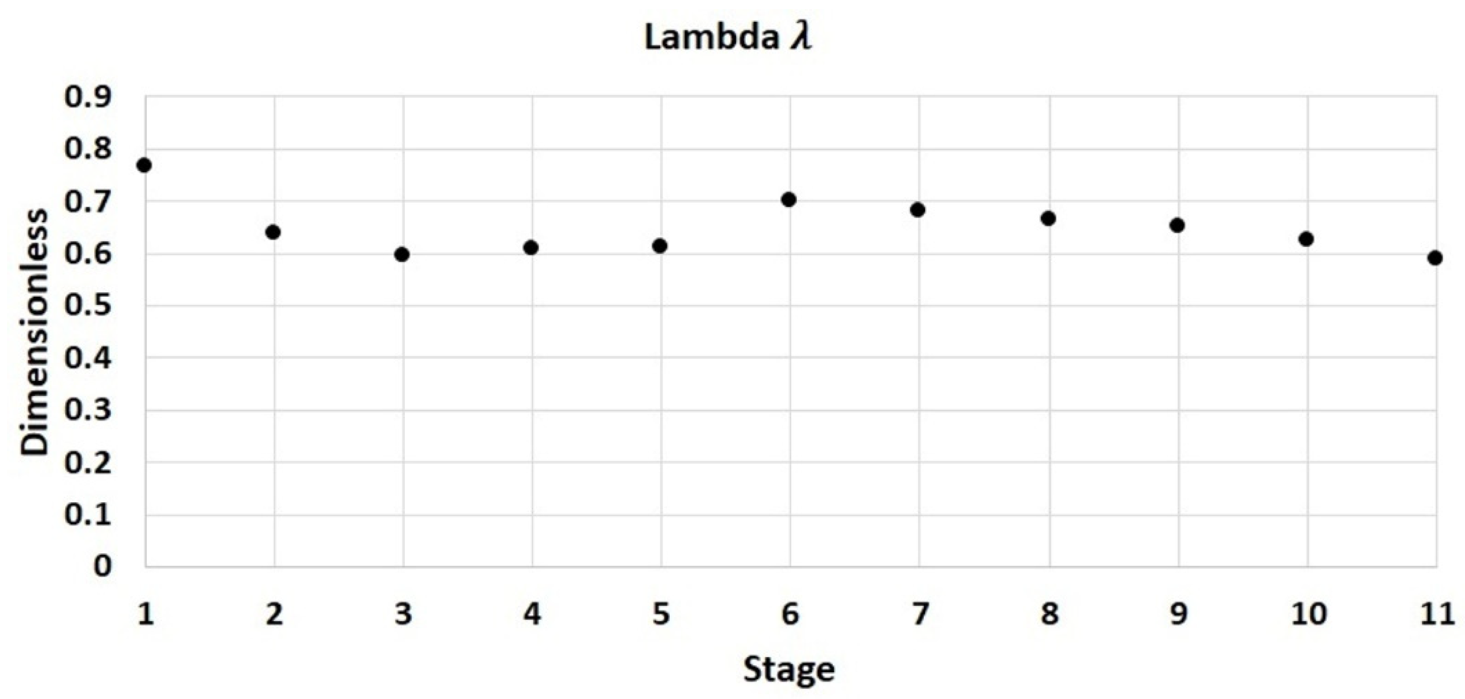
A constant efficiency η is considered in the calculation of pressure ratio across the stages (Equation (2)). The efficiency η is obtained from a 0-D model of compressor map (pressure ratio and speed as input and efficiency as output) related to the 11-stage axial compressor considered in this study. Schnoes et al. [25] estimated the efficiency η across the stages of a 15-stage axial compressor using throughflow analysis and demonstrated a variation of the efficiency η across the different stages. In this study, a constant efficiency η is considered in the calculation of pressure ratio (Equation (2)). The parameter λ in Equation (2) accounts for the variation of efficiency η across the stages to match the pressure ratio estimated from HFDT and estimated by Equation (2).
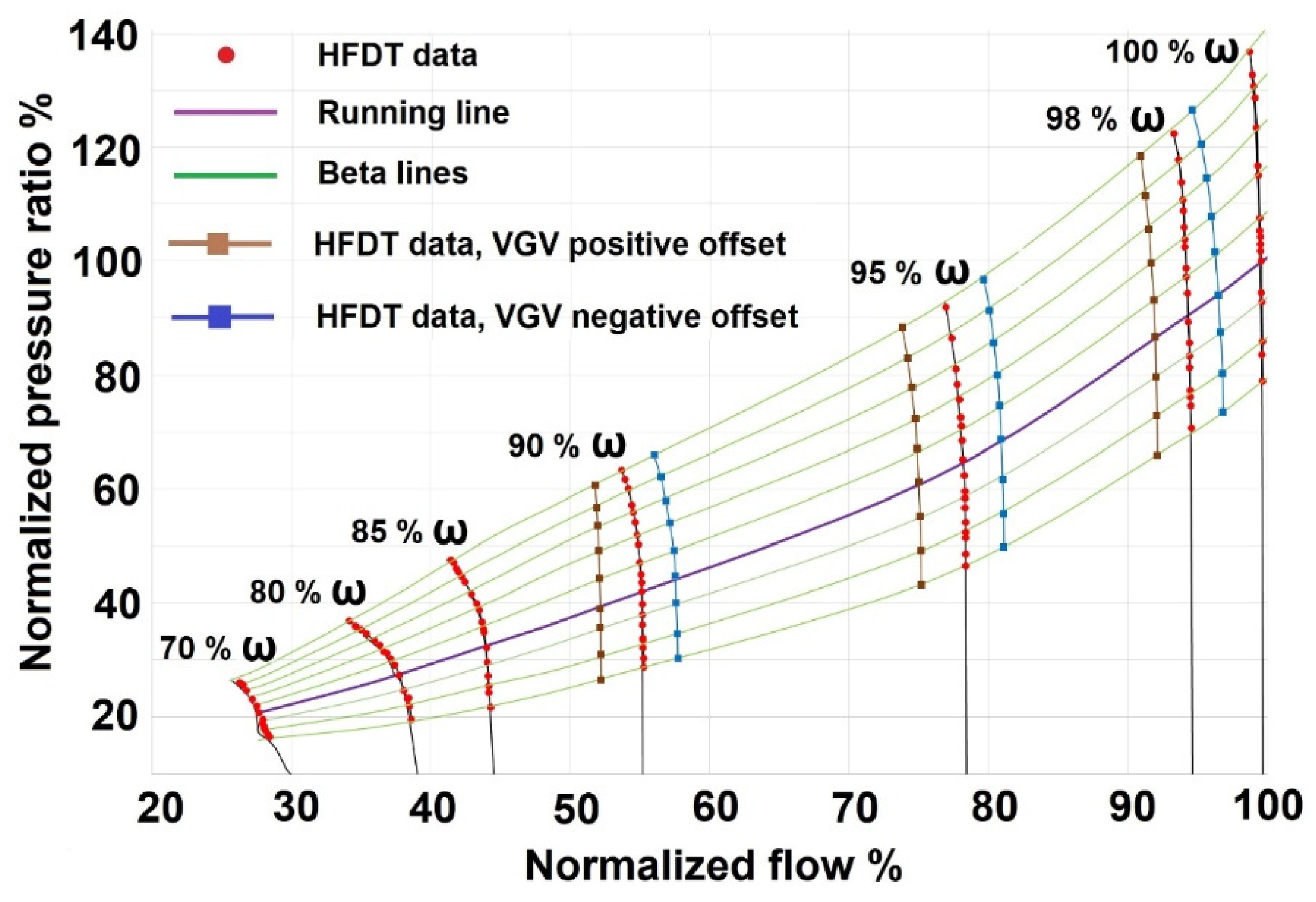
In this study, the pressure ratio for each stage has also been collected from the HFDT during compressor simulation at different rotational speeds and at a different offset in the IGV position. Stagewise pressure ratio collected from the HFDT allows the validation of the compressor model at steady-state conditions. This has been demonstrated in a previous study [21]. The IGV demand angle was scheduled with respect to compressor speed. The position (in degrees) of VGVs is a function of IGV position. An offset in the IGV position is considered as a position of the IGV outside its scheduled position with respect to the GGS. Figure 1 shows the total pressure ratio calculated by the HFDT and represented in the overall compressor performance map of an 11-stage axial compressor. The compressor map was validated with real-world compressor data. The total pressure ratio estimated from the HFDT is calculated by multiplying the individual pressure ratio across the stages comprising the 11-stage axial compressor. The compressor map shown in Figure 1 considers 9 “beta lines” across each speed. These beta lines will allow the interpolation of pressure ratio between different speeds and flow rates during the dynamic compressor simulation. The running line representing the overall operating range of the compressor is shown in Figure 1. It shows the total pressure ratio vs. flow rate at different operational speeds. The pressure ratio and flow rate were normalized with respect to the pressure ratio and flow rate values at 100% speed and at nominal conditions. The operational speed was normalized with respect to the maximum speed ωmax. Figure 1 also shows the pressure ratio calculated by the HFDT and considering an offset in the position of the VGVs outside its nominal scheduled position with respect to GGS.
The 1-D modeling procedure can be executed in the Matlab® environment. It consists of an optimization process to estimate the parameter λ and a calculation process to predict stagewise temperature and pressure ratio. More information about the optimization process and calculation process from the 1-D compressor modeling architecture can be found in the previous study [21]. White et al. [26] presented a flow diagram to depict the 1-D modeling architecture of a multistage axial compressor. Their modeling architecture considers subroutines and estimates the blade angles across the stages in the compressor to predict overall compressor performance maps. This is in contrast to this study in which the geometry of the 11-stage compressor was provided by the compressor manufacturer.
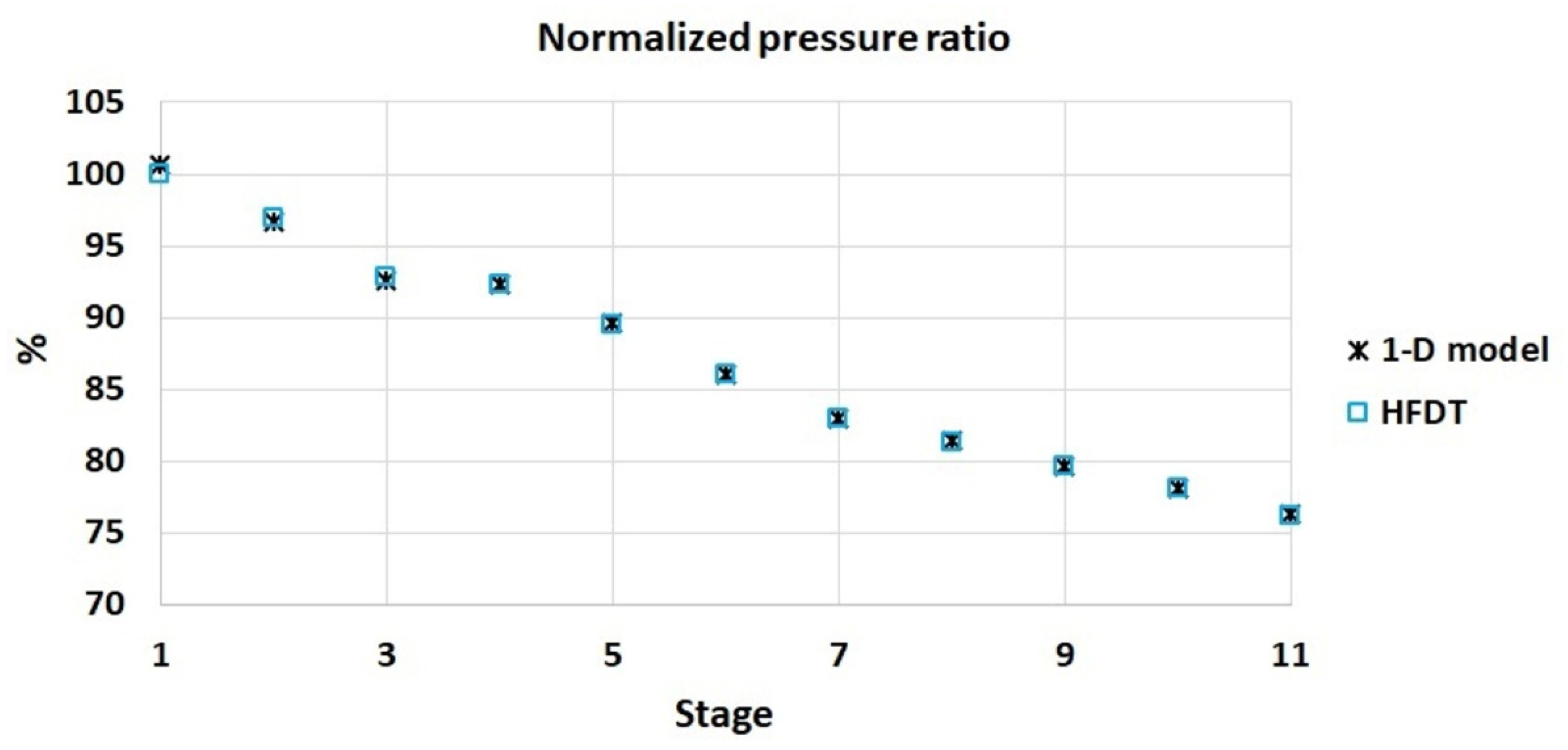
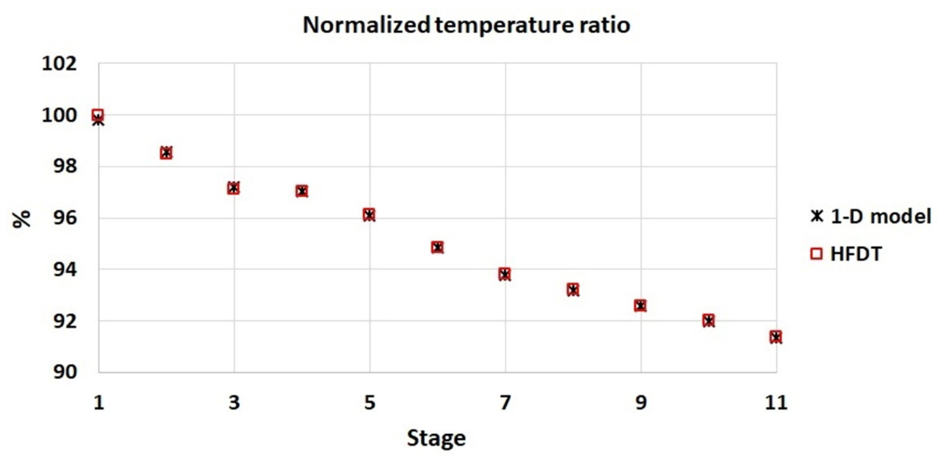
Figure 2 shows the estimation of the parameter λ related to the performance running line (Figure 1) at 100% rotational speed and considering the optimization process from the 1-D compressor modeling architecture [21]. Figure 3 and Figure 4 show the resulting stagewise pressure and temperature ratio calculated from the parameter λ and Equations (1) and (2) and considering the calculation process. The pressure and temperature ratio shown in Figure 3 and Figure 4 were normalized with respect to the maximum value of the HFDT stagewise data from the total pressure ratio of the compressor performance running line (design point) at 100% rotational speed.
3. Engine Modeling Architecture
A 0-D engine model constructed in a Simulink environment [23] was considered for the simulation of the dynamic compressor performance of a twin-shaft IGT system at different load conditions.
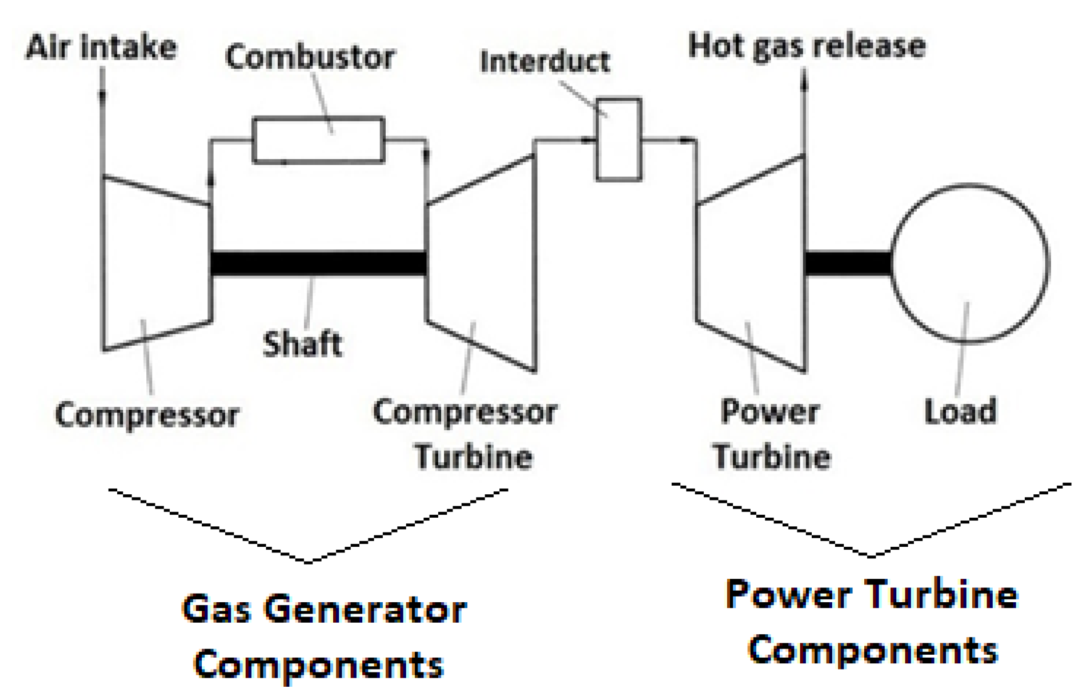
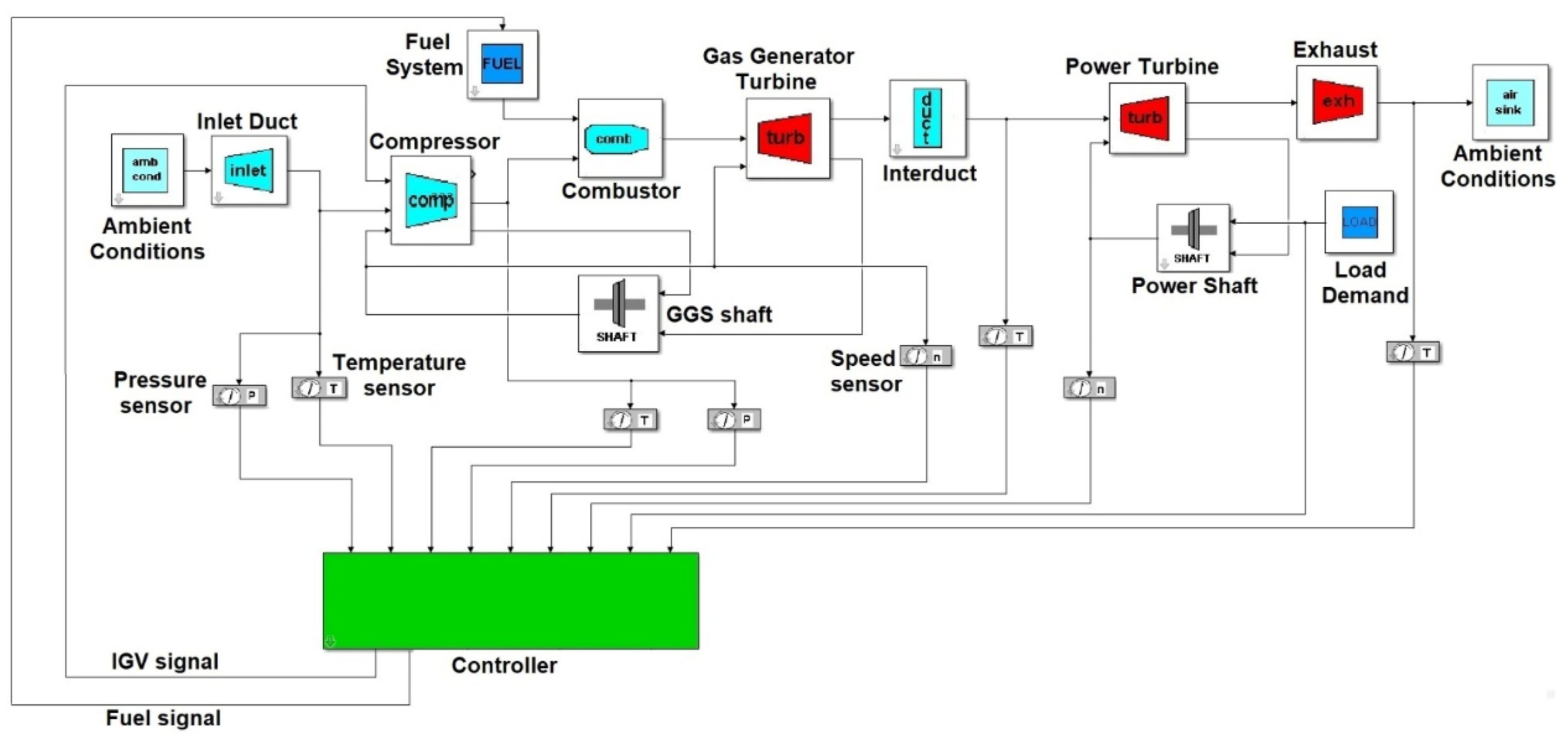
The 0-D twin-shaft engine model comprises gas generator components and power turbine components, and they are connected through an interduct component. The gas generator components comprise the compressor, combustor, gas generator turbine (GGT), and a shaft connecting the compressor and GGT, as shown in Figure 5. Power turbine components comprise the power-turbine (PT), load, and mechanical shaft connecting the PT and load. As inputs, the model requires the load and the temperature and pressure of the air entering the compressor. Conservation of mechanical energy for shafts, heat-soaking effects for metal parts, and conservation of thermodynamic energy are included in the component models. The dynamic model of the gas turbine engine can be expressed with a system of nonlinear differential equations. The following equation is considered to model the dynamic response of pressure in the individual model components:
where ςj is the internal thermodynamic state. The first term on the right-hand side of Equation (3) represents volume gas dynamics, and the second term on the right-hand side describes the behavior of components using nonlinear algebraic equations. More details of Equation (3) and the differential equations representing the dynamic model of the twin-shaft gas turbine were reported in the study of Panov [23].
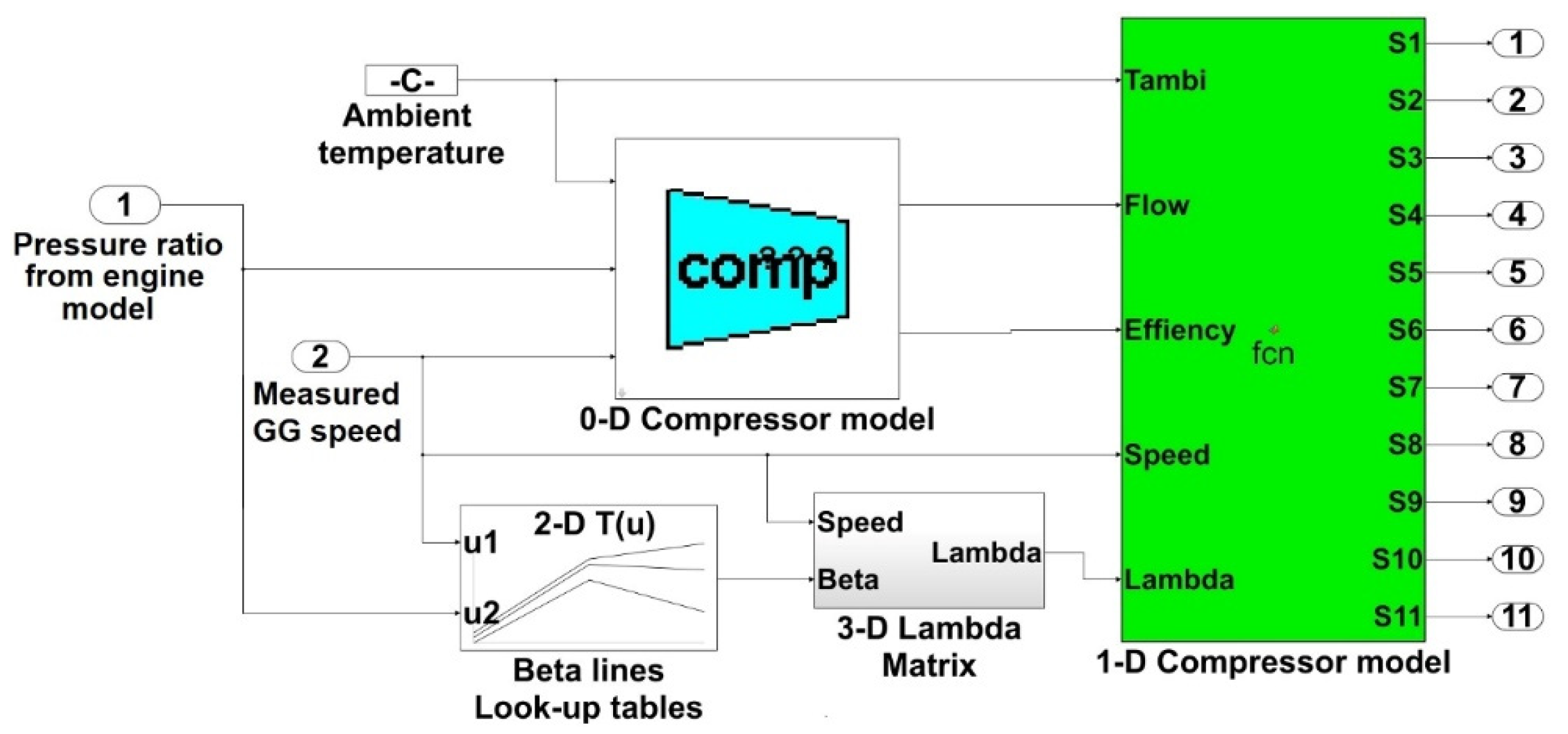
The 0-D modeling architecture comprises a lumped axial compressor model and considers compressor performance maps for flow and efficiency as a function of pressure ratio and rotational speed. The 0-D engine model can predict the total flow, efficiency, pressure and temperature of air discharged by the compressor at steady and transient conditions. The normalized compressor flow map defined in the 0-D compressor model is shown in Figure 1. As discussed in the previous section, the 1-D model requires as inputs the temperature at ambient conditions, the airflow rate, efficiency, speed and lambda (λ work-done factor) values. The 0-D compressor developed in the Simulink environment [23] is interfaced with the 1-D model, as shown in Figure 6. The modeling architecture presented in this study combines the 1-D compressor model reported in a previous study [21] and developed in the Matlab® with the 0-D twin-shaft gas turbine model developed in the Simulink environment and reported by Panov [23]. As shown in Figure 6, both modeling architectures can be interfaced in the Simulink environment by feeding parameters from the 0-D twin-shaft engine model into the 1-D compressor model. The 1-D model requires flow, efficiency, and speed from the 0-D compressor (twin-shaft gas turbine model) and calculates the pressure and temperature rising across the different stages of the multistage axial compressor.
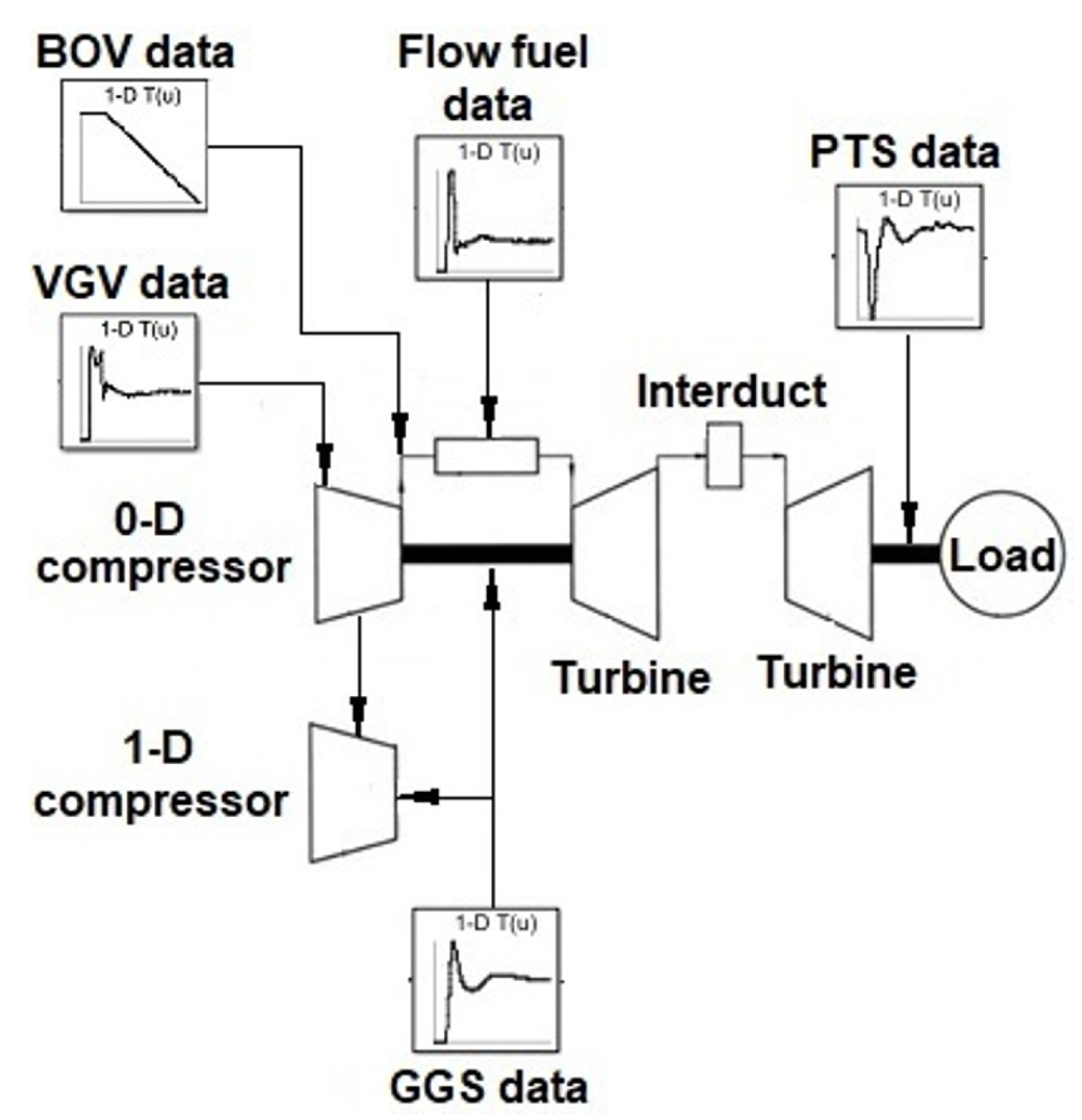
Values of the parameter λ are required in the 1-D compressor model, as discussed in the previous Section 2. A 3-D matrix defined in the Simulink environment was defined to include all the values of the parameter λ. The 3-D matrix calculates 11 values for λ from a given speed, a given value of IGV offset and a defined point on the beta line from the compressor map shown in Figure 1. The calculated vector of λ values is provided to the 1-D model to calculate stagewise pressure and temperature across the 11 stages of the compressor. The overall modeling architecture comprises the 0-D engine model and the 1-D compressor model, as shown in Figure 7.
The gas turbine data measured during the engine test of a twin-shaft IGT are provided to the different components of the 0-D engine model. The deployed gas turbine 0-D model does not contain a control system and mechanical system components such as the GG shaft and the PT shaft. Therefore, GGS, power turbine speed (PTS) and control system variables such as fuel flow demand (FFDEM), VGV demand (VGVDEM) and bleed\blow-off valve demand (BOVDEM) positions are provided to the 0-D gas turbine as a time history obtained from engine test. The engine model calculates the pressure ratio of the 0-D compressor model from the measured engine data and provides the flow to the 1-D compressor model. The 1-D model calculates the dynamic inter-stage compressor performance at different engine load conditions. This will be demonstrated in the results section.
4. Compressor Dynamic Validation
Measured engine data from a twin-shaft gas turbine operated during load acceptance test were considered for the validation of the developed model. The engine test data were logged during a step change in engine load from 13% to 40% of the maximum engine load. Two sets of measurements when increasing engine load from 13% to 40% were considered. The first set of measurements considers engine operation with air bleed from center-casing for the purpose of emission control–CO turndown. The second set of measurements was taken during engine operation without air bleed, which corresponds to natural turndown engine operation. In addition, measurements during engine tests with center-casing air bleed during load acceptance from 26% to 53% of the maximum load have also been considered.
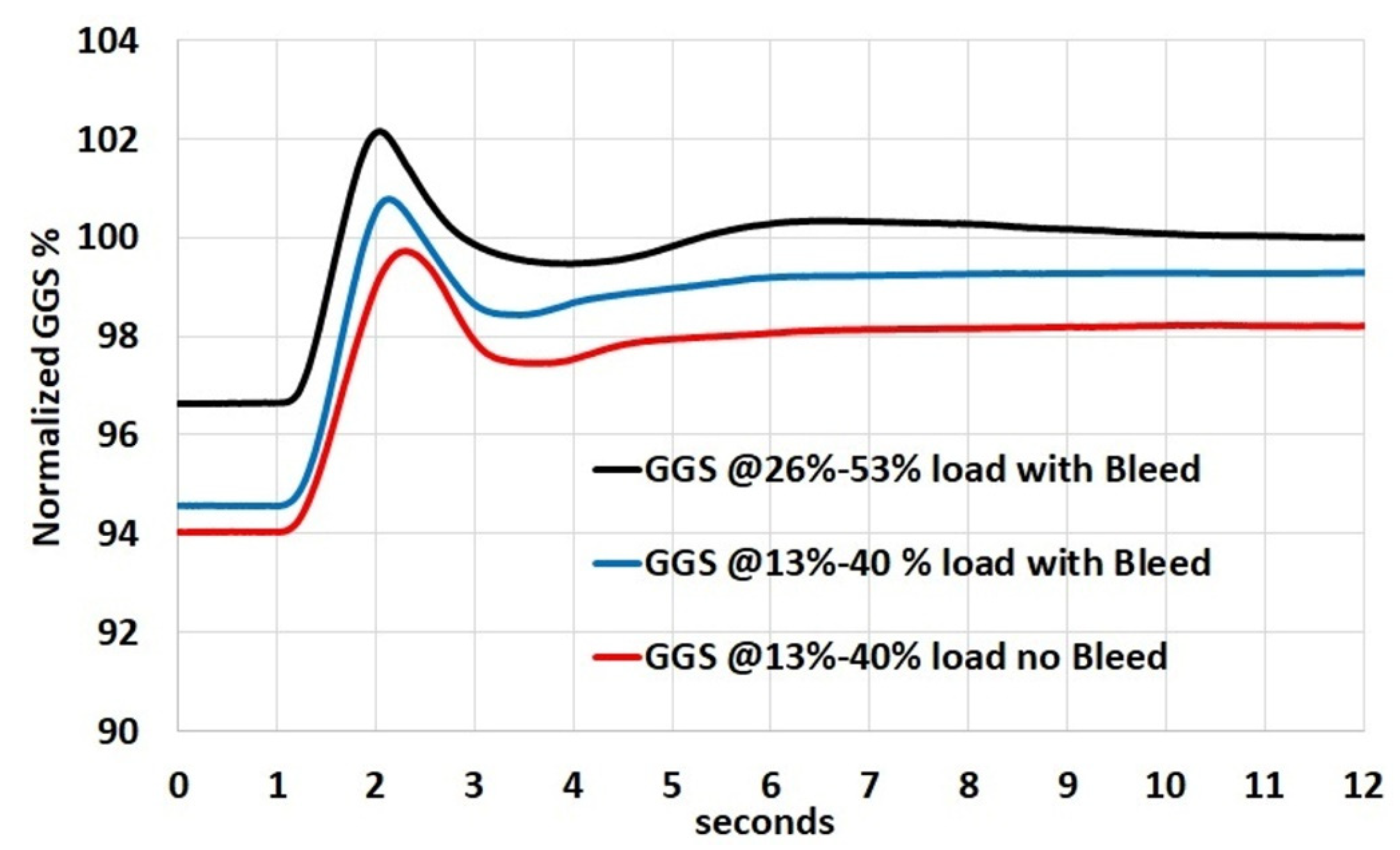
The engine data comprise FFDEM, GGS, PTS, VGVDEM position, BOVDEM position and compressor discharge pressure (CDP). The FFDEM, BOVDEM, VGVDEM, GGS and PTS data are considered as inputs in the modeling architecture as shown in Figure 7. The measured CDP allowed the validation of the compressor model. Figure 8 shows the normalized GGS with respect to the measured GGS at steady-state at 53% load. A decrease in measured GGS is observed when no air bled from center-casing is considered, and with increasing load demand from 13% to 40%.
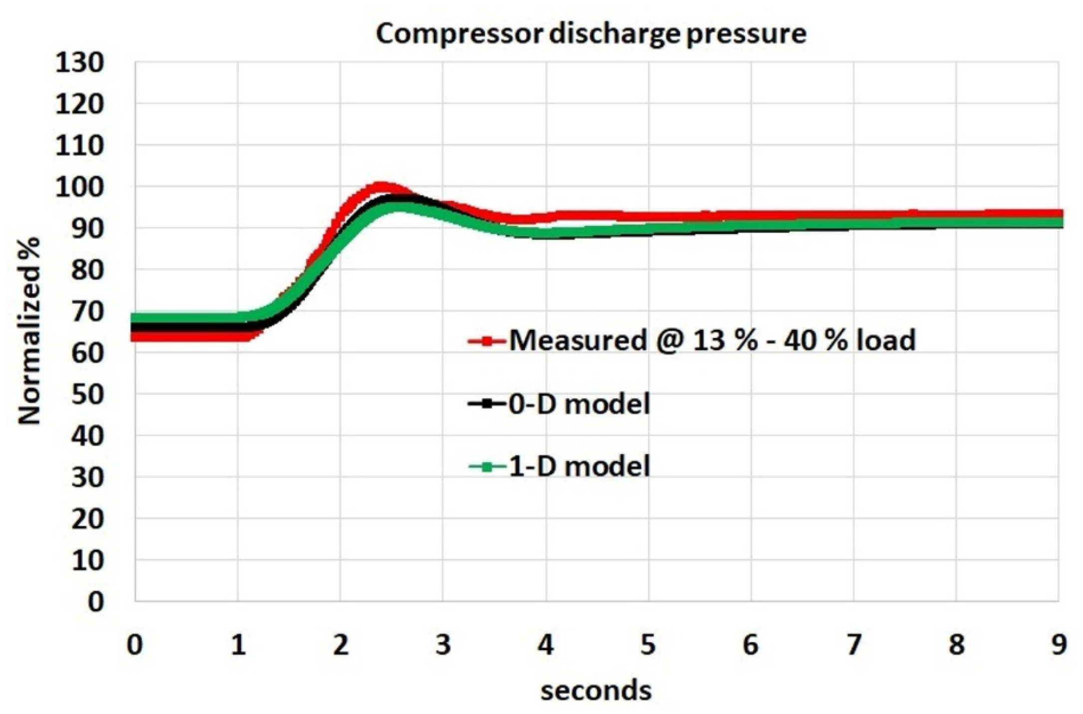
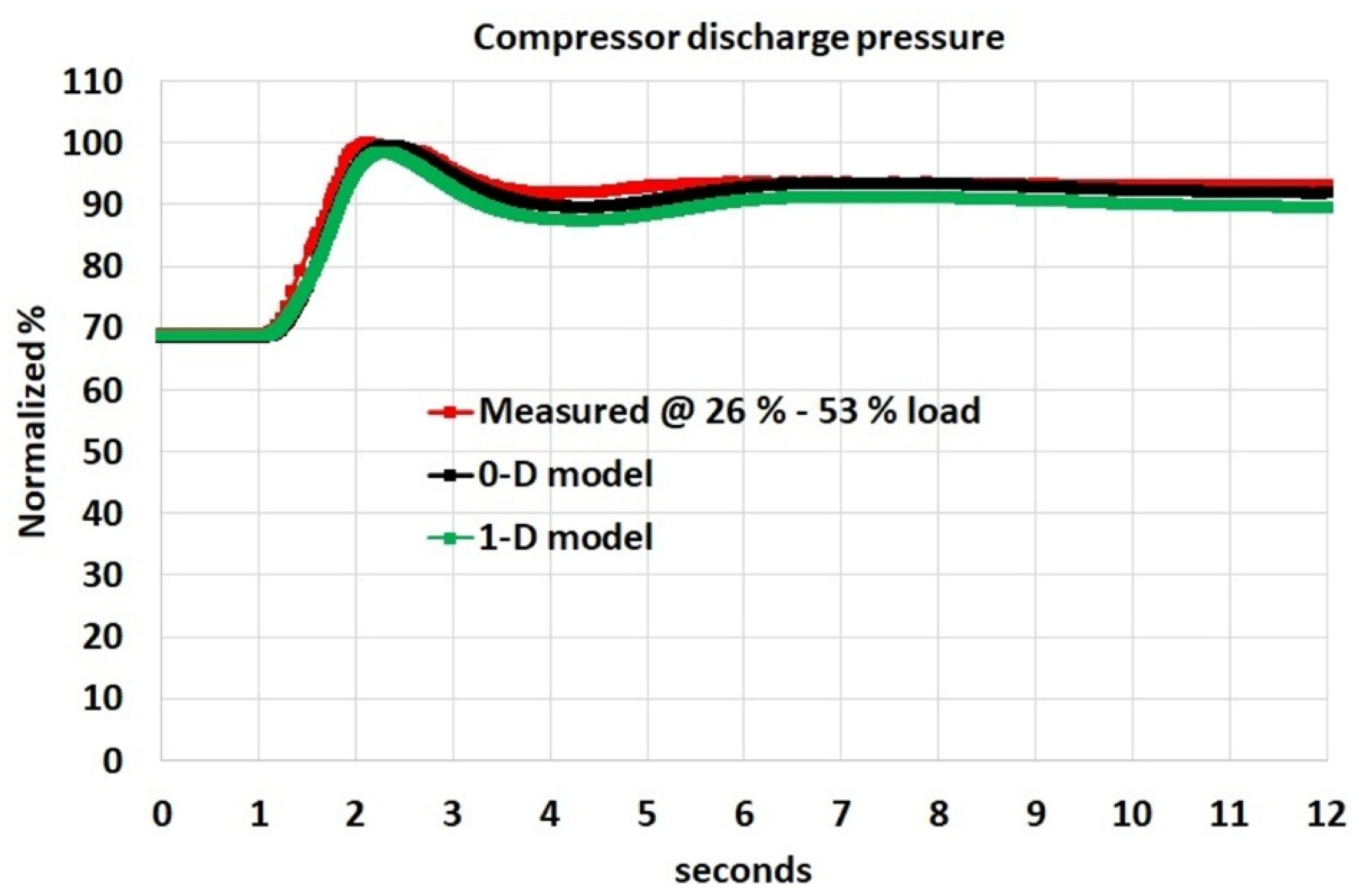
Figure 9 and Figure 10 show a comparison between the measured CDP and the predicted CDP from the 0-D and 1-D compressor models. The volume gas dynamic expressed in Equation (3) was considered in the 0-D compressor model to simulate the transient response of the CDP, as shown in Figure 9 and Figure 10. The interaction between the 0-D and 1-D compressor models is shown in Figure 6. The 1-D compressor model requires as inputs the air mass flow and efficiency calculated by the 0-D compressor model and calculates the stagewise pressure ratio across the 11 stages. The total pressure ratio estimated by the 1-D model is calculated by multiplying all the individual stagewise pressure ratio across the 11 stages. In addition, pressure loss related to the compressor diffuser and outlet guide vanes was considered to approximate the simulated 1-D compressor model response with the measured data.
Table 1 shows the error between the 0-D compressor model and measured data. The error between the 1-D compressor model and measured data are also shown in Table 1. The error in the 1-D compressor model is higher than the error in the 0-D compressor model. From Figure 9 and Figure 10, it can be observed that the biggest discrepancy between the measured data and the 1-D compressor model is during the dynamic response. This is considered to be due to the steady nature of losses predicted by HFDT steady-state calculations. The 1-D compressor model was developed from the HFDT tool, which represents the performance of the multiaxial compressor at steady-state conditions. The increase in error between the simulated data from the 1-D model and the measured data during transient engine performance is mainly attributed to the fact that the 1-D model cannot accurately predict the measured data at transient conditions. The 1-D model was developed using simulated data from the HFDT, as shown in Figure 1. The HFDT data represent the performance of the compressor at steady-state conditions.
5. Results
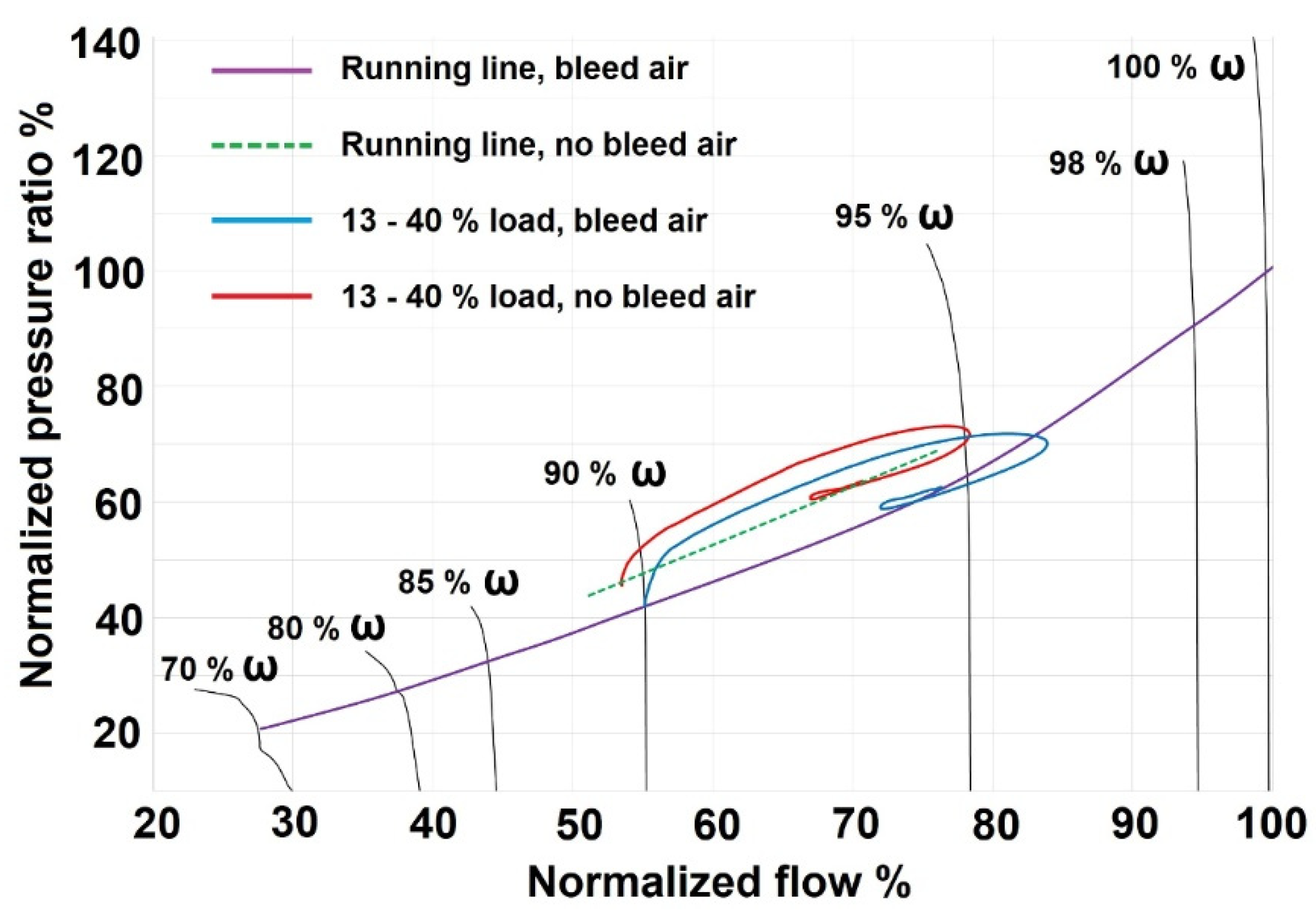
The transient compressor responses previously described in the validation section can be represented on the overall compressor map. Figure 11 shows the compressor transient excursion when the engine load is increased from 13% to 40% of the maximum load with and without center casing bleed. Figure 11 shows the effect of air bleeding during compressor operation on the compressor component map. The compressor transient excursion neglecting the air bleed effect is drifted towards the stability line.
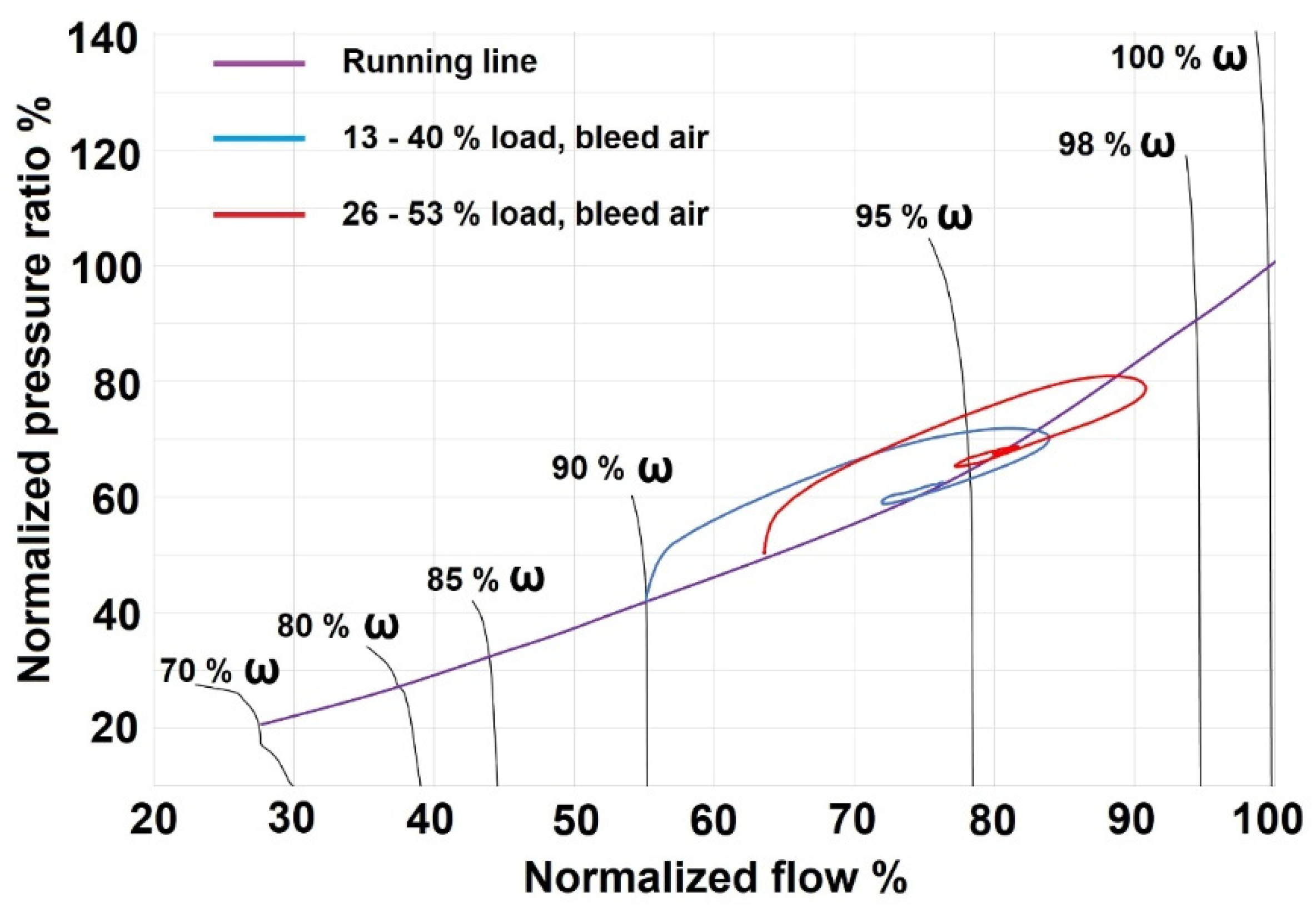
The transient response during load acceptance maneuver from 13–40%, and 26% to 53% with center case bleed effect is shown in Figure 12.
5.1. Offset in IGV Position
The position of the VGVs is a function of the IGV position. An offset in the IGV position is considered as a position outside of its scheduled position with respect to the GGS. A positive IGV offset position closes the VGVs, and a negative IGV offset position opens the VGVs. The engine model, constructed using specialized Simulink library reported by Panov [23], is considered for the simulation of the engine performance with an offset in the IGV position of the axial compressor. A controller implemented within the engine model, as shown in Figure 13, regulates the amount of fuel demand with respect to the temperature and pressure from the different stations of the engine and load demand.
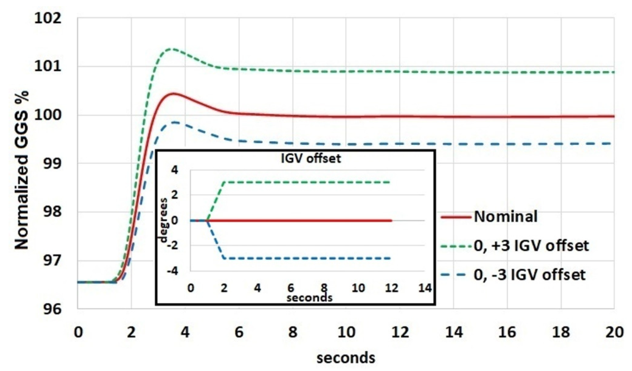
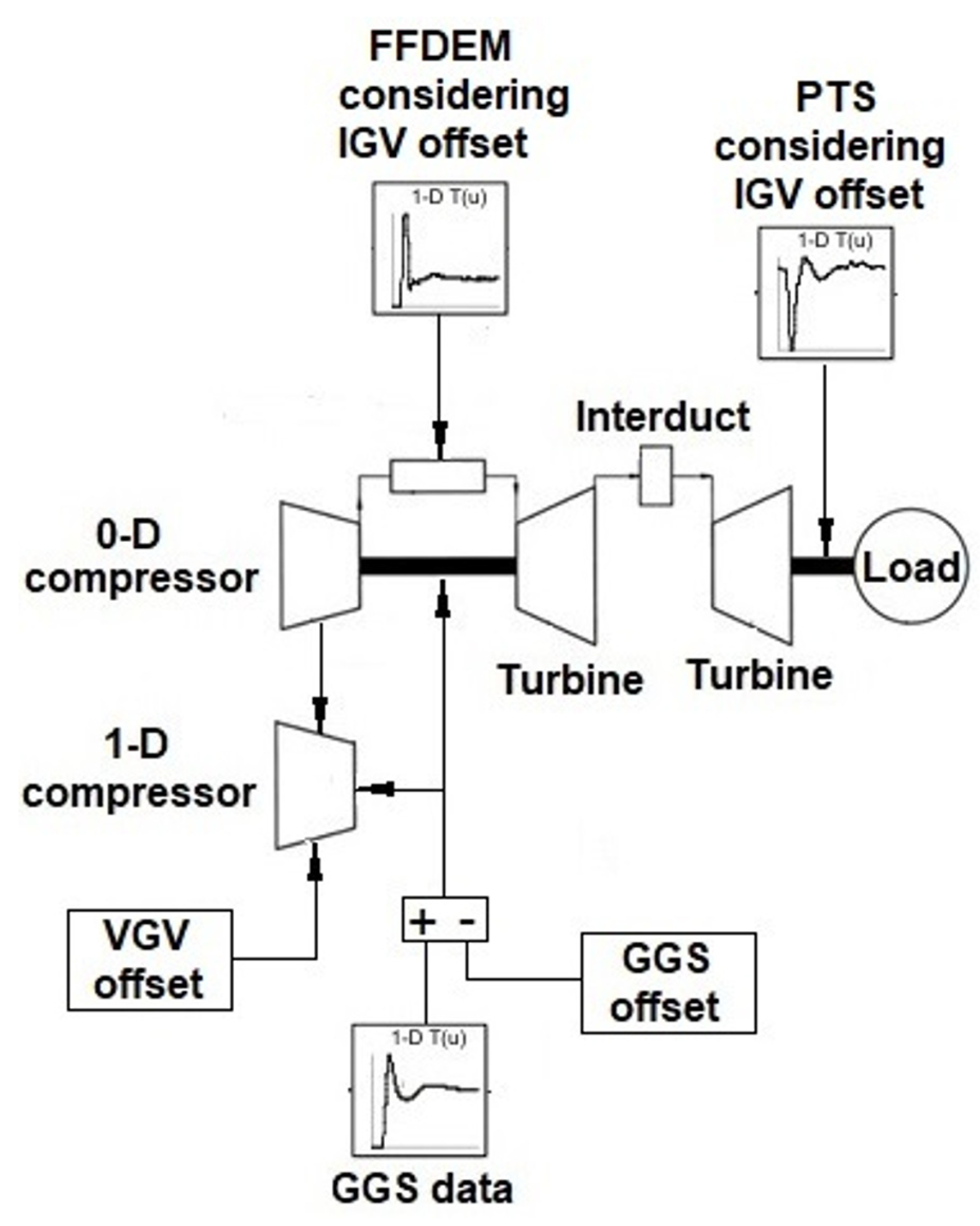
The engine model shown in Figure 13 was tuned to predict the steady-state response of the compressor (start and endpoints of transient excursion) shown in Figure 12 when the engine load was increased from 26–53% of the maximum load. A positive offset of 3 degrees and a negative offset of 3 degrees in the IGV position at 53% of the load was considered during engine simulation. A nominal position in the IGV (scheduled IGV position for that GGS) was considered at 26% load. Figure 14 shows the simulated GGS when the load is increased from 26–53% load and considering the positive and negative offset of 3 degrees in the IGV position at 53% load. The simulated GGS shown in Figure 14 was normalized with respect to the GGS at 53% load and at nominal conditions. Figure 14 shows an increase in the GGS when a positive offset of 3 degrees is considered in the IGV position. A decrease in the GGS is also shown in Figure 14, when a negative offset of 3 degrees is considered in the IGV position. The difference in GGS for negative and positive IGV offset position with respect to the nominal condition shown in Figure 14 is coined as GGS offset. The GGS offset value is implemented in the engine modeling structure previously shown in Figure 7 to simulate the effect of the IGV offset position on the compressor performance map. The engine modeling architecture is constructed in the Simulink environment. It is possible to add or subtract values between the signals connecting the different modules in the Simulink environment. The GGS offset value is added to the signal connecting the look-up table for the measured GGS at nominal conditions and the engine model, as shown in Figure 15. In addition, the simulated signals for FFDEM and PT speed at positive and negative IGV offset are considered in the engine model shown in Figure 15.
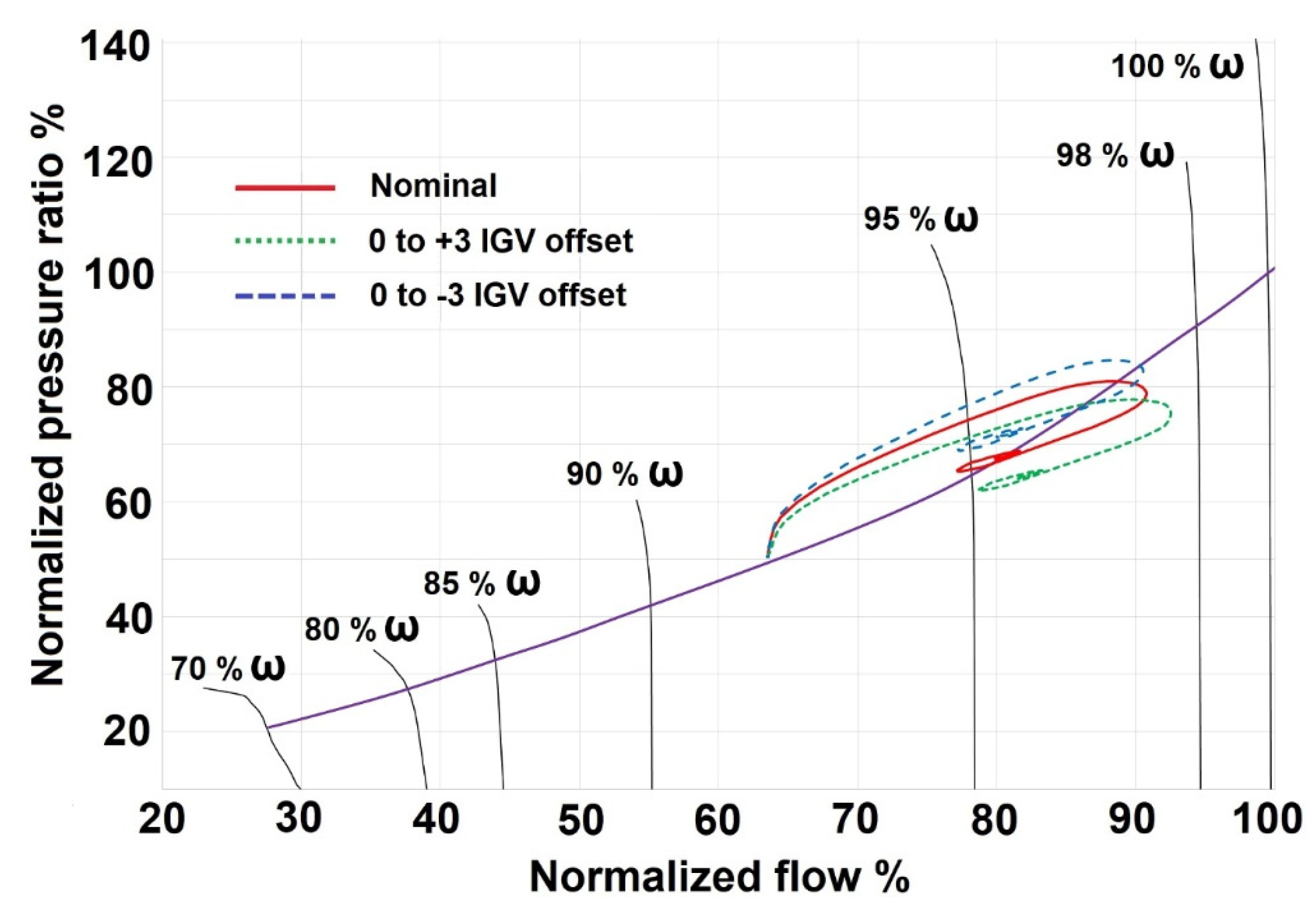
Figure 16 shows the simulated compressor performance considering positive and negative offset of 3 degrees in the IGV position at 53% load. An increase in pressure ratio when considering a negative offset in the IGV position (opening VGVs) is observed in Figure 16. A decrease in pressure ratio when considering a positive IGV offset position (closure of VGVs) is shown in Figure 16 as well. Hashmi et al. [27] simulated the effect of VGV drift in a low-pressure compressor (LPC) on a three-shaft gas turbine (GE LM1600). The results demonstrated that an updrift schedule (positive offset) in the VGV position decreased the pressure discharge by the LPC, and a downdrift schedule (negative offset) increase the LPC pressure discharge. Urasek et al. [28] reported that by closing the IGV and VGVs for a given speed in an axial flow compressor, the total pressure ratio is decreased.
5.2. Inter-Stage Dynamic Performance Simulation
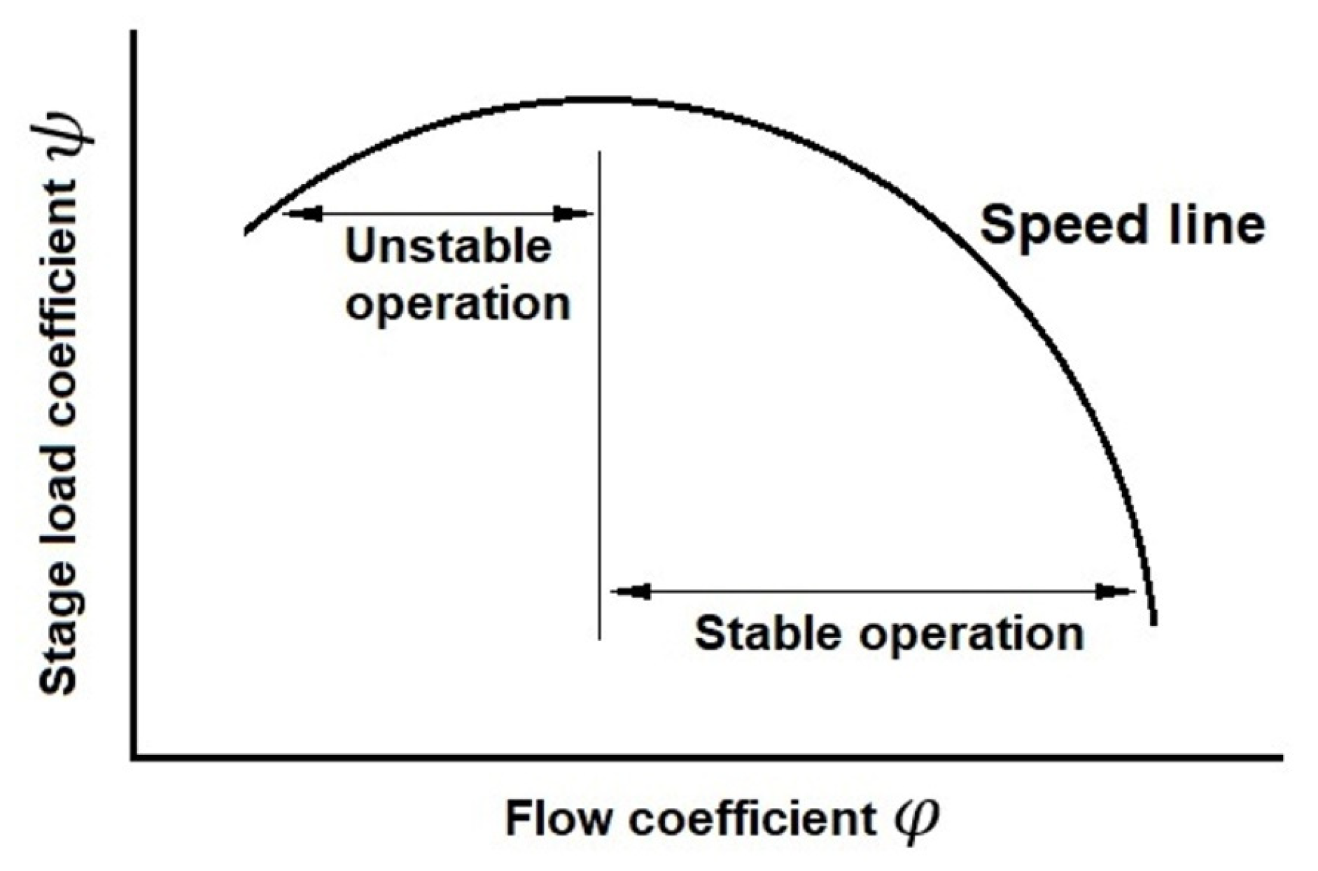
A representation of a stage performance map is shown in Figure 17. The stage performance map is comprised of two regions: stable and unstable operation. Ideally, a compressor is designed to operate on the stable operation region, but under certain conditions, the compressor operation may be drifted towards the stability limit condition. The use of VGVs and air bleed during compressor operation can ensure that compressor can operate with sufficient stability margin. The compressor stage performance map represented in Figure 17 can allow the assessment of the dynamic compressor performance at different engine load conditions. The use of stage-characteristic maps to assess compressor performance was considered in different studies [20,29,30,31].
The equations to predict the flow and load coefficients for the stage performance map shown in Figure 17 are:
where Equation (4) is defined as the flow coefficient
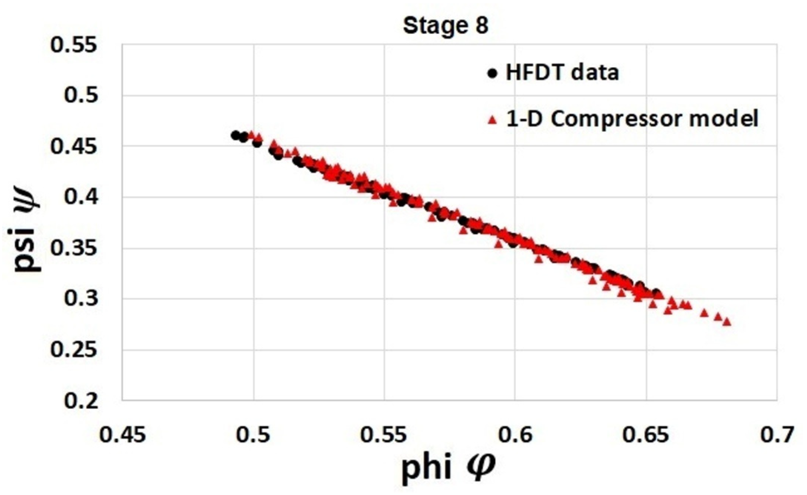
and Equation (5) is the load coefficient. The nomenclature of Equations (4) and (5) was described in Section 2 on theory. The 1-D compressor model can predict the stage-characteristic maps predicted by the HFDT data using Equations (4) and (5) describing the flow and load coefficients. Figure 18 shows a comparison between the stage-performance map (Stage 8) predicted by the HFDT and by the 1-D compressor model. Figure 18 shows that the flow coefficients and load coefficients calculated by Equations (4) and (5) from 70–100% speed follow the same trend [32].
5.2.1. Center-Casing Bleed Effect
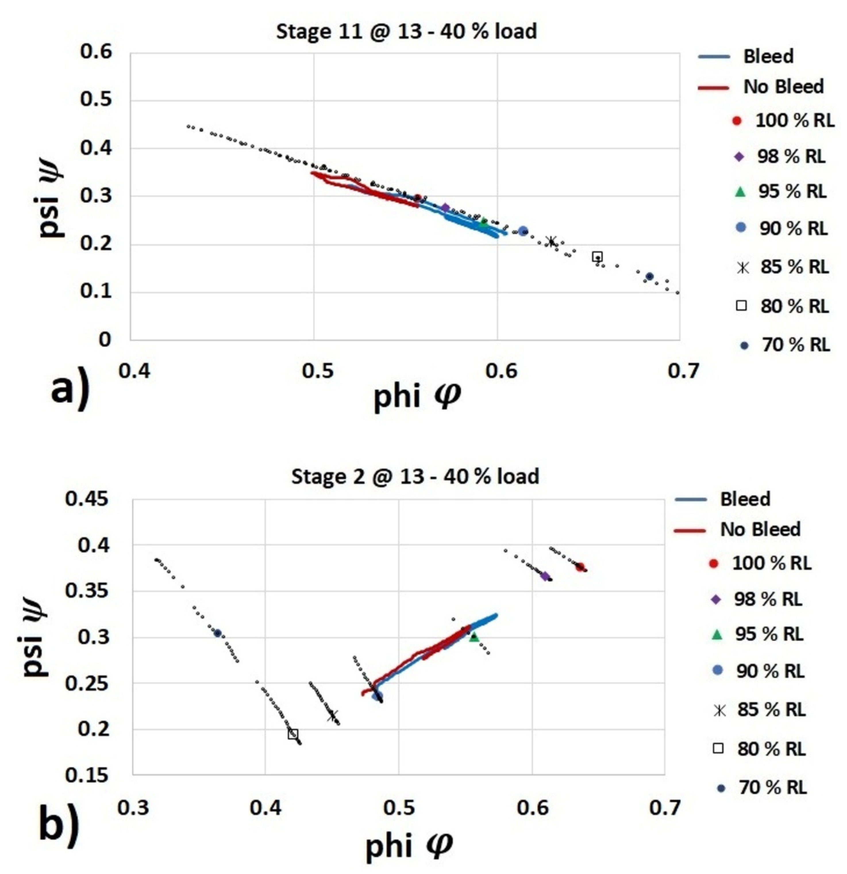
The transient compressor responses shown in Figure 11, Figure 12 and Figure 16 can also be represented in the individual stage performance maps. The transient compressor response on the individual stage-characteristics map does not consider phenomena related to the individual compressor stage, e.g., transient heat transfer [33] and stage tip clearance [34]. Figure 19 shows the transient response of the compressor on the stage characteristic map when the engine load is increased from 13% to 40% of the maximum load with and without center-casing bleed. The 1-D model calculates the stage-characteristic maps predicted by the HFDT, as demonstrated in Figure 18. It can be observed in Figure 19a that the stage performance of stage-11 at all speeds collapse together [32]. The stage-11 performance associated with the running line (RL) considering air bleed and for all speeds is also shown in Figure 19a. This figure demonstrates that the compressor operates on stable conditions when the air bleed effect is considered. As the load is increased from 13 to 40%, the transient compressor response is moving towards the reduced flow coefficient φ and towards the stability limit of the stage characteristic map. The transient compressor response that neglects air bleed approaches closer to the stability limit, as shown in Figure 19a. Figure 19b shows the stage characteristic map associated with the second stage. The calculated flow and load coefficients associated with the second stage are sparse and do not collapse into a single trend. This could be associated with different compressor geometry attributed to the VGVs located at the front-end of the compressor. Figure 19b shows that the transient compressor response is moving towards the increased flow coefficient φ with increasing load from 13–40%. As expected, the transient compressor response that does not consider air bleed moves closer towards the stability limit and above the response that considers air bleed.
5.2.2. Load Effect
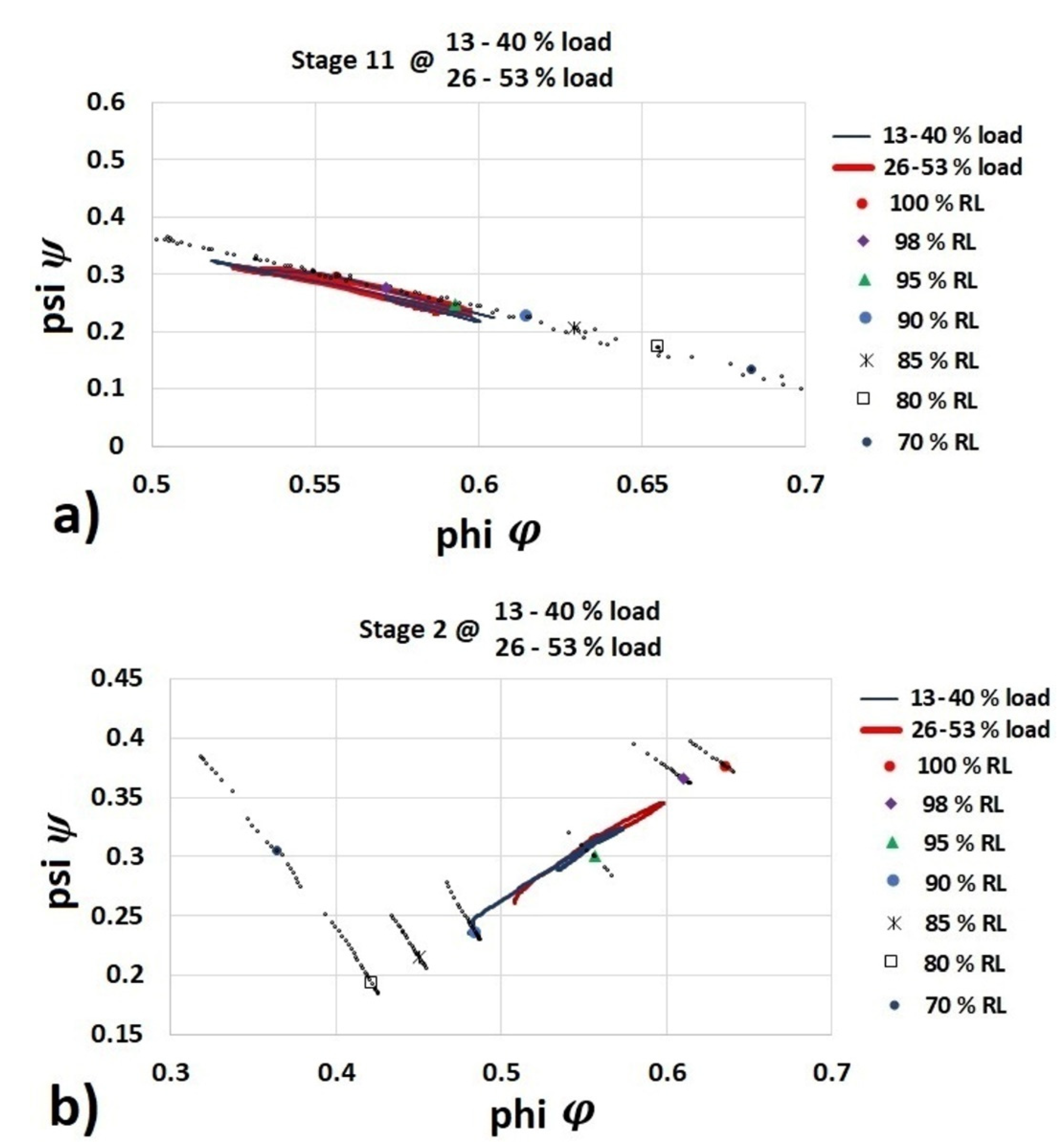
The transient compressor response when the engine load is increased from 13% to 40% and from 26 to 53% load and considering CO Turndown operation effect is shown in Figure 20. Figure 20a shows that the transient compressor response for the case at 13–40% load is moving towards the reduced flow coefficient φ or towards the stability limit of the stage characteristic map compared to the transient compressor response for the case at 26–53% load. Figure 20b shows that the transient compressor response at higher load is shifted towards the increased flow coefficient φ– higher load conditions.
5.2.3. IGV Offset Effect
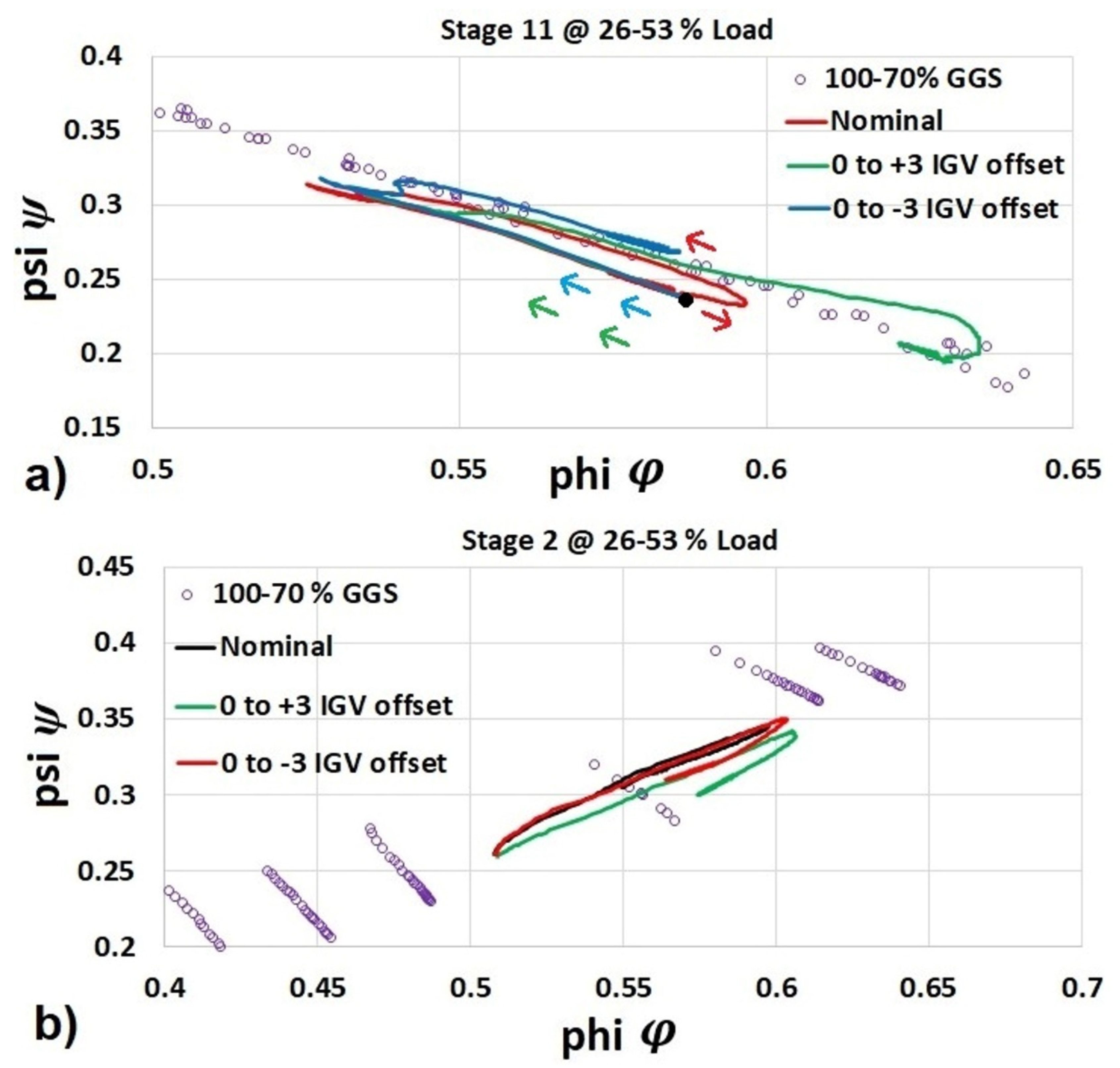
Figure 21 shows the transient response of the compressor on the stage characteristic map when the engine load is increased from 26% to 53% of the maximum load at nominal IGV position and with an offset in the IGV position at 53% load. As the load is increased from 26% to 53%, the transient compressor response is moving towards the reduced flow coefficient φ and towards the stability limit of the stage characteristic map as shown in Figure 21a. The steady-state flow coefficient at 53% load increases when considering a positive IGV offset (endpoint of the green line) and moves away from the stability limit in the stage-performance map. This effect can also be corroborated in the overall compressor map shown in Figure 16, considering the typical compressor stability margin for the case at positive IGV offset. Figure 21b shows the stage characteristic map associated with the second stage. Figure 21b shows that the transient compressor response is moving towards the increased flow coefficient φ with increasing load from 26–53%. As expected, the transient compressor response that considers positive IGV offset moves away from the stability limit and below the nominal transient compressor response.
This study has integrated the 1-D compressor model developed in a previous study [21] within a whole gas turbine model [23] containing 0-D component models to predict the inter-stage dynamic compressor performance at load acceptance maneuvers and with an offset in IGV position. In addition, the effect of the center-casing air bleed was analyzed on the overall compressor map and stage-characteristic maps. At low speeds and considering no center-casing air bleed, a given stage may be performed close to its stability limit, which could cause instability of the whole compressor during the dynamic engine operation. The transient compressor response exhibits operation with a higher stability margin when the center-casing air bleed effect is active. A higher stability margin on the overall compressor map and stage-characteristic maps is also predicted when closing VGVs (positive offset in IGV position) during compressor operation. In the previous study [21], the effect of IGV mal-function and the effect of fouling on stagewise performance at steady-state conditions were demonstrated. The deposition of dirt and dust particles on the compressor blades increases surface roughness on the blades and changes the velocity triangles representing the compressor blades [35]. The dynamic change in flow capacity and efficiency in the compressor during fouling conditions and during VGV malfunction was simulated through a Simulink 0-D gas turbine model [36]. In future work, the developed modeling architecture from this study will simulate and validate the dynamic stagewise performance during compressor fouling conditions and VGV malfunction.
6. Conclusions
A semi-empirical 1-D modeling framework comprising theoretical relations, design parameters, and stagewise data of a multistage axial compressor was integrated with a 0-D engine model developed in the Simulink environment. The overall modeling architecture was validated with engine test data of a twin-shaft gas turbine measured during the load acceptance maneuvers. The engine test data comprise data measured during the load step change and considering natural and CO turndown engine operation. The modeling architecture was able to predict the measured transient response of the compressor discharge pressure with step-change of engine load and considering and neglecting center-casing air bleed effect. The effect of the center-casing air bleed was analyzed on the overall compressor map and stage-characteristic maps. Further analysis by considering an offset in the IGV position with respect to its scheduled position with GGS was carried out. The effect of offset in the IGV position on compressor performance was demonstrated in the overall compressor map and stage-characteristic maps. The transient compressor response exhibits operation with a higher stability margin when the center-casing air bleed effect is active and with closing the VGVs (positive offset in IGV position). This study has demonstrated that it is possible to analyze the dynamic performance of the compressor during the transition between two operating conditions by assessing the stability margin at a given compressor stage. The developed theoretical framework can provide a better prediction of dynamic compressor performance, especially during transient engine operation, at which the compressor running line may get closer to its stability limit.
Author Contributions
Conceptualization, V.P.; formal analysis, S.C.-M.; funding acquisition, C.B.; methodology, V.P., S.K.; supervision, S.K., V.P.; validation, S.C.-M.; writing—original draft, S.C.-M.; writing—review and editing, S.K., V.P. and C.B. All authors have read and agreed to the published version of the manuscript.
Funding
This research was funded by Siemens Energy Industrial Turbomachinery Ltd., Lincoln. The APC was funded by Siemens Energy Industrial Turbomachinery Ltd., Lincoln.
Acknowledgments
The authors would like to thank Siemens Energy Industrial Turbomachinery Ltd., Lincoln, U.K., for providing research support and access to real-world data to support the research outcomes.
Conflicts of Interest
The authors declare no conflict of interest.
Nomenclature
| List of Symbols | |
| A | annulus area (m2) |
| CP | heat capacity at constant pressure (J/kgK) |
| CX | air axial velocity (m/s) |
| air flow rate (kg/s) | |
| PR | pressure ratio (dimensionless) |
| r | radius of the annulus (m) |
| U | blade velocity (m/s) |
| T | temperature (K) |
| Greek | |
| α | air angle from the axial direction |
| λ | work-done factor (dimensionless) |
| η | polytropic efficiency (dimensionless) |
| air density kg/m3 | |
| γ | heat capacity ratio (dimensionless) |
References
- Razak, V.A. Industrial Gas Turbines Performance and Operability; Woodhead Publishing Limited: Cambridge, UK, 2007; ISBN 978-1-84569-205-6. [Google Scholar]
- Muir, D.E.; Saravanamutto, H.I.H.; Marshall, D.J. Health Monitoring of Variable Geometry Gas Turbines for Canadian Navy. J. Eng. Gas Turbines Power 2009, 111, 244–250. [Google Scholar] [CrossRef]
- Tournier, J.-M.; El-Genk, M.S. Axial flow, multi-stage turbine and compressor models. Energy Convers. Manag. 2010, 51, 16–29. [Google Scholar] [CrossRef]
- Johnson, M.S. One-Dimensional, Stage-by-Stage, Axial Compressor Performance Model. In Proceedings of the ASME 1991 International Gas Turbine and Aeroengine Congress and Exposition, Orlando, FL, USA, 3–6 June 1991. Paper No: 91-GT-192, V001T01A070. [Google Scholar] [CrossRef] [Green Version]
- Dong, Y.; Zheng, X.; Li, Q. An 11-stage axial compressor performance simulation considering the change of tip clearance in different operating conditions. Proc. IMechE Part A J. Power Energy 2014, 228, 614–625. [Google Scholar] [CrossRef]
- Alm-Eldien, A.M.; Gawad, A.F.A.; Hafaz, G.; Kreim, M.G.A.E. Design and Optimization of a Multi-Stage Axial-Flow Compressor. In Proceedings of the Eleventh International Conference of Fluid Dynamics, Alexandria, Egypt, 19–21 December 2013. Paper No: ICFD11-EG-4103. [Google Scholar]
- Song, T.W.; Kim, T.S.; Kim, J.H.; Ro, S.T. Performance prediction of axial flow compressors using stage characteristics and simultaneous calculation of interstage parameters. Proc. Inst. Mech. Eng. 2001, 215, 89–98. [Google Scholar] [CrossRef]
- Tsalavoutas, A.; Mathioudakis, K.; Stamatis, A.; Smith, M. Identifying Faults in the Variable Geometry System of a Gas Turbine Compressor. J. Turbomach. 2000, 123, 33–39. [Google Scholar] [CrossRef] [Green Version]
- Hosseini, S.H.R.; Khaledi, H.; Ghofrani, M.B. Model Based Compressor Fault Identification Using Stage Stacking Technique and Nonlinear Diagnostic System. In Proceedings of the ASME Turbo Expo 2008: Power for Land, Sea, and Air, Berlin, Germany, 9–13 June 2008. Paper No: GT2008-51032, 213-221. [Google Scholar]
- Schulte, H.; Schmidt, K.J.; Weckend, A.; Staudacher, S. Multi Stage Compressor Model for Transient Performance Simulations. In Proceedings of the ASME Turbo Expo 2008: Power for Land, Sea, and Air, Berlin, Germany, 9–13 June 2008; Paper No: GT2008-51159. pp. 185–195. [Google Scholar] [CrossRef]
- Tsoutsanis, E.; Meskin, N. Derivative-driven window-based regression method for gas turbine performance prognostics. Energy 2017, 128, 302. [Google Scholar] [CrossRef] [Green Version]
- Tsoutsanis, E.; Meskin, N.; Benammar, M.; Khorasani, K. Dynamic Performance Simulation of an Aeroderivative Gas Turbine Using the Matlab Simulink Environment. In Proceedings of the ASME 2013 International Mechanical Engineering Congress and Exposition, San Diego, CA, USA, 15–21 November 2013. Paper No. IMECE2013-64102, V04AT04A050. [Google Scholar] [CrossRef]
- Patel, V.C.; Kadirkamanathan, V.; Thompson, H.A.; Fleming, P.J. Utilising a Simulink gas turbine engine model for fault diagnosis. In Proceedings of the IFAC Symposium on Control of Power Plants and Power Systems, Cancún, Mexico, 6–8 December 1995; Volume 28, pp. 237–242. [Google Scholar] [CrossRef]
- Asgari, H.; Venturini, M.; Chen, X.; Sainudiin, R. Modeling and Simulation of the Transient Behavior of an Industrial Power Plant Gas Turbine. J. Eng. Gas Turbines Power 2014, 136, 061601. [Google Scholar] [CrossRef]
- Watanabe, M.; Ueno, Y.; Mitani, Y.; Iki, H.; Uriu, Y.; Urano, Y. A dynamical model for customer’s gas turbine generator in industrial power systems. IFAC Proc. 2009, 42, 203–208. [Google Scholar] [CrossRef]
- Yu, Y.; Chen, L.; Sun, F.; Wu, C. Matlab/Simulink-based simulation for digital-control system of marine three-shaft gas-turbine. Appl. Energy 2005, 80, 1–10. [Google Scholar] [CrossRef]
- Gobran, M.H. Off-design performance of solar Centaur-40 gas turbine engine using Simulink. Ain. Shams Eng. J. 2013, 4, 285–298. [Google Scholar] [CrossRef] [Green Version]
- Srikanth, K.S.; Naresh, K.; Narasimha, L.V.; Ramesh, V. Matlab/Simulink Based Dynamic Modeling of Microturbine Generator for Grid and Islanding Modes of Operation. Int. J. Power Syst. 2016, 1, 1–6. [Google Scholar]
- Cruz-Manzo, S.; Panov, V.; Zhang, Y.; Latimer, A.; Agbonzikilo, F. A thermodynamic transient model for performance analysis of a twin shaft Industrial Gas Turbine. In Proceedings of the ASME Turbo Expo 2017, Charlotte, NC, USA, 26–30 June 2017. Paper No. GT2017-64376, V006T05A020. [Google Scholar] [CrossRef]
- Damiani, L.; Crosa, G.; Trucco, A. A Control Oriented Simulation Model of a Multistage Axial Compressor. In Proceedings of the Ecos 2012—The 25th International Conference on Efficiency, Cost, Optimization, Simulation and Environmental Impact of Energy Systems, Perugia, Italy, 26–29 June 2012. [Google Scholar]
- Cruz-Manzo, S.; Krishnababu, S.; Panov, V.; Zhang, Y. Performance calculation of a multi-stage axial compressor through a semi-empirical modelling framework. In Proceedings of the Global Power and Propulsion Society 2019, Beijing, China, 16–18 September 2019. Paper No. GPPS-BJ-2019-123. [Google Scholar]
- Wu, C.H. A General Theory of Three-Dimensional Flow in Subsonic and Supersonic Turbomachines of Axial-, Radial-, and Mixed-Flow Types; NACA TN 2604; National Advisory Committee for Aeronautics: Cleveland, OH, USA, 1952. [Google Scholar]
- Panov, V. GasTurbolib-Simulink Library for Gas Turbine Engine Modelling. In Proceedings of the ASME Turbo Expo 2009, Orlando, FL, USA, 8–12 June 200; Paper No. GT2009-59389. pp. 555–565. [Google Scholar] [CrossRef]
- Saravanamuttoo, H.; Rogers, G.; Cohen, H.; Straznicky, P. Gas Turbine Theory, 6th ed.; Prencice Hall: Upper Jersey River, NJ, USA, 2009. [Google Scholar]
- Schnoes, M.; Voß, C.; Nicke, E. Design optimization of a multi-stage axial compressor using throughflow and a database of optimal airfoils. J. Glob. Power Propuls Soc. 2018, 2, 516–528. [Google Scholar] [CrossRef]
- White, N.M.; Tourlidakis, A.; Elder, R.L. Axial compressor performance modelling with a quasi-one-dimensional approach. Proc. Inst. Mech. Eng. Part A J. Power Energy 2002, 216, 181–193. [Google Scholar] [CrossRef]
- Hashmi, M.B.; Lemma, T.A.; Karim, Z.A.A. Investigation of the combined effect of variable inlet guide vane drift, fouling, and inlet air cooling on gas turbine performance. Entropy 2019, 21, 1186. [Google Scholar] [CrossRef] [Green Version]
- Urasek, D.C.; Steinke, R.J.; Cunnan, W.S. Stalled and Stall-Free Performance of Axial-Flow Compressor Stage with Three Inlet-Guide-Vane and Stator-Blade Settings; NTRS-NASA Technical Reports Server, NASA-TN-D-8457; NASA: Washington, DC, USA, 1977. [Google Scholar]
- Wentong, M.; Yongwen, L.; Ming, S.; Nanhua, Y. Multi-stage axial flow compressors characteristics estimation based on system identification. Energy Convers. Manag. 2008, 49, 143–150. [Google Scholar]
- Howell, A.R.; Bonham, R.P. Overall and stage characteristics of axial flow compressors. Proc. Inst. Mech. Eng. 1950, 163, 235–248. [Google Scholar] [CrossRef]
- Mellor, G.L.; Root, T. Generalized Multistage Axial Compressor Characteristics, ASME. J. Basic Eng. 1961, 83, 709–718. [Google Scholar] [CrossRef]
- Pampreen, R.C. Compressor Surge and Stall; Concepts ETI, Inc.: Norwich, VT, USA, 1993. [Google Scholar]
- Kiss, A.; Spakovszky, Z. Effects of transient heat transfer on compressor stability. J. Turbomach. 2018, 140, 121003. [Google Scholar] [CrossRef] [Green Version]
- Larjola, J. Simulation of Surge Margin Changes Due to Heat Transfer Effects in Gas Turbine Transients. Int. J. Turbo Jet Engines 1985, 2, 81–92. [Google Scholar] [CrossRef]
- Tarabrin, A.P.; Bodrov, A.I.; Schurovsky, V.A.; Stalder, J.-P. Influence of Axial Compressor Fouling on Gas Turbine Unit Performance Based on Different Schemes and with Different Initial Parameters. In Proceedings of the ASME International Gas Turbine and Aeroengine Congress, Stockholm, Sweden, 2–5 June 1998. ASME Paper No. 98-GT-416. [Google Scholar] [CrossRef] [Green Version]
- Cruz-Manzo, S.; Panov, V.; Zhang, Y. Gas Path Fault and Degradation Modelling in Twin-Shaft Gas Turbines. Machines 2018, 6, 43. [Google Scholar] [CrossRef] [Green Version]
Figure 1.
Pressure ratio estimated by high-fidelity design tool (HFDT) in overall compressor performance map.
Figure 1.
Pressure ratio estimated by high-fidelity design tool (HFDT) in overall compressor performance map.

Figure 2.
Estimation of parameter λ from HFDT at design point and 100% ωmax.

Figure 3.
Comparison between stagewise pressure ratio from the 1-D model and HFDT at design point and 100% ωmax.
Figure 3.
Comparison between stagewise pressure ratio from the 1-D model and HFDT at design point and 100% ωmax.

Figure 4.
Comparison between stagewise temperature ratio from the 1-D model and HFDT at design point and 100% ωmax.
Figure 4.
Comparison between stagewise temperature ratio from the 1-D model and HFDT at design point and 100% ωmax.

Figure 5.
Representation of 0-D engine model developed in the Simulink environment.

Figure 6.
Interface between 0-D and 1-D compressor models in the Simulink environment.

Figure 7.
Overall modeling architecture for dynamic simulation of compressor performance.

Figure 8.
Normalized gas generator speed (GGS) considered as input in the engine model.

Figure 9.
Compressor discharge pressure with increasing load from 13% to 40% of the maximum load and with no bleed.
Figure 9.
Compressor discharge pressure with increasing load from 13% to 40% of the maximum load and with no bleed.

Figure 10.
Compressor discharge pressure with increasing load from 26% to 53% of the maximum load and considering bleed.
Figure 10.
Compressor discharge pressure with increasing load from 26% to 53% of the maximum load and considering bleed.

Figure 11.
Representation of transient compressor response on compressor performance map for 13–40% load with/without bleed air.
Figure 11.
Representation of transient compressor response on compressor performance map for 13–40% load with/without bleed air.

Figure 12.
Representation of transient compressor response on compressor performance map for 13–40% load and 26–53% load with bleed air.
Figure 12.
Representation of transient compressor response on compressor performance map for 13–40% load and 26–53% load with bleed air.

Figure 13.
Simulink model for simulation of engine performance with inlet guide vane (IGV) offset position.
Figure 13.
Simulink model for simulation of engine performance with inlet guide vane (IGV) offset position.

Figure 14.
Simulated GGS response for 26–53% load and considering a positive and negative IGV offset of 3 degrees at 53% load.
Figure 14.
Simulated GGS response for 26–53% load and considering a positive and negative IGV offset of 3 degrees at 53% load.

Figure 15.
Engine model considering a GGS change during offset in IGV position.

Figure 16.
Simulated compressor dynamic response for 26–53% load and considering positive and negative IGV offset of 3 degrees at 53% load.
Figure 16.
Simulated compressor dynamic response for 26–53% load and considering positive and negative IGV offset of 3 degrees at 53% load.

Figure 17.
Representation of stage performance map.

Figure 18.
Comparison between stage-performance map (stage 8) predicted by HFDT and predicted by 1-D compressor model from 70–100% speed.
Figure 18.
Comparison between stage-performance map (stage 8) predicted by HFDT and predicted by 1-D compressor model from 70–100% speed.

Figure 19.
Compressor transient response on the stage characteristic map @ 13–40% load and with/without bleed air, (a) stage 11, (b) stage 2.
Figure 19.
Compressor transient response on the stage characteristic map @ 13–40% load and with/without bleed air, (a) stage 11, (b) stage 2.

Figure 20.
Transient compressor response on the stage characteristic map @ 13–40% load and 26–53% load with bleed air, (a) stage 11, (b) stage 2.
Figure 20.
Transient compressor response on the stage characteristic map @ 13–40% load and 26–53% load with bleed air, (a) stage 11, (b) stage 2.

Figure 21.
Simulated compressor dynamic response on stage performance map for 26–53% load and considering positive and negative IGV offset of 3 degrees at 53% load, (a) stage 11, (b) stage 2.
Figure 21.
Simulated compressor dynamic response on stage performance map for 26–53% load and considering positive and negative IGV offset of 3 degrees at 53% load, (a) stage 11, (b) stage 2.


Table 1.
Average error in simulated compressor discharge pressure from 0-D and 1-D compressor models.
Table 1.
Average error in simulated compressor discharge pressure from 0-D and 1-D compressor models.
| Load | % Error Bleed | % Error No Bleed | ||
|---|---|---|---|---|
| 0-D Model | 1-D Model | 0-D Model | 1-D Model | |
| 13–40% | 1.11 | 3.07 | 2.95 | 4.24 |
| 26–53% | 1.13 | 3.05 | - | - |
Publisher’s Note: MDPI stays neutral with regard to jurisdictional claims in published maps and institutional affiliations. |
© 2020 by the authors. Licensee MDPI, Basel, Switzerland. This article is an open access article distributed under the terms and conditions of the Creative Commons Attribution (CC BY) license (http://creativecommons.org/licenses/by/4.0/).
Share and Cite
MDPI and ACS Style
Cruz-Manzo, S.; Krishnababu, S.; Panov, V.; Bingham, C. Inter-Stage Dynamic Performance of an Axial Compressor of a Twin-Shaft Industrial Gas Turbine. Machines 2020, 8, 83. https://doi.org/10.3390/machines8040083
AMA Style
Cruz-Manzo S, Krishnababu S, Panov V, Bingham C. Inter-Stage Dynamic Performance of an Axial Compressor of a Twin-Shaft Industrial Gas Turbine. Machines. 2020; 8(4):83. https://doi.org/10.3390/machines8040083
Chicago/Turabian StyleCruz-Manzo, Samuel, Senthil Krishnababu, Vili Panov, and Chris Bingham. 2020. "Inter-Stage Dynamic Performance of an Axial Compressor of a Twin-Shaft Industrial Gas Turbine" Machines 8, no. 4: 83. https://doi.org/10.3390/machines8040083
Note that from the first issue of 2016, this journal uses article numbers instead of page numbers. See further details here.