Parallel Direct and Iterative Methods for Solving the Time-Fractional Diffusion Equation on Multicore Processors

Abstract

The work is devoted to developing the parallel algorithms for solving the initial boundary problem for the time-fractional diffusion equation. After applying the finite-difference scheme to approximate the basis equation, the problem is reduced to solving a system of linear algebraic equations for each subsequent time level. The developed parallel algorithms are based on the Thomas algorithm, parallel sweep algorithm, and accelerated over-relaxation method for solving this system. Stability of the approximation scheme is established. The parallel implementations are developed for the multicore CPU using the OpenMP technology. The numerical experiments are performed to compare these methods and to study the performance of parallel implementations. The parallel sweep method shows the lowest computing time.

1. Introduction

The last decades have seen the significant rise of interest to the time-fractional differential equations [1,2,3,4,5]. This is due to possibility to use these equations for modeling the multiple phenomena of anomalous diffusion and other processes with memory effects. Multiple experimental researches [6,7,8] showed that the assumption of the Brownian motion in the diffusion processes may not be sufficient for the accurate description of some physical processes. The fractional differential equations are the powerful mathematical tool for adequate description of many real physical processes, and their application field still grows. The qualitive and quantitative aspects of analysis of these nonlocal models are quite complex for researching.

Thus, development of the efficient numerical algorithms for solving the direct and inverse problems for fractional differential equations is of considerable theoretical and practical interest today.

For solving approximately the initial-boundary problems for the time-fractional diffusion equation, one can use various numerical techniques. The sufficient review is presented in works [9,10,11]. The most popular methods are: the finite difference method, finite element method, spectral methods, and meshless techniques. The numerical methods for solving the fractional differential equations are quite expensive due to nonlocal properties of the fractional derivatives. Thus, development of the efficient numerical algorithms is a crucially important problem. The promising way to solve various compute-intensive problems is parallel computing [12,13,14,15,16,17,18]. Several parallel algorithms has been developed specifically for the fractional differential equations and anomalous diffusion problems [19,20].

In work [21], for solving the SLAE with tridiagonal matrix, the parallel direct algorithm was implemented. It is based on: partitioning the matrix into blocks, processing the blocks separately on different processors, and obtaining the final solution by solving the reduced system.

In work [22], the parallel algorithms were constructed for solving a two-dimensional partial differential equation with the Riemann–Liouville time derivatives. For solving the SLAEs arising in this problem, the iterative Krylov subspace methods were used, namely, the generalized method of minimal residuals, quasiminimal residual method, and induced dimension reduction method. Parallelization was performed by distributing the computation between threads.

In our work, we construct the parallel algorithm for solving the one-dimensional time-fractional diffusion equation (TFDE). The implicit finite difference approximation reduces the equation to a large system of linear algebraic equations. Three algorithms are applied to solving this system, namely, the direct Thomas algorithm, the direct parallel sweep method, and the iterative accelerated over-relaxation method. The parallel algorithms are implemented on the multicore processors using the OpenMP technology. To assess the efficiency of the developed parallel algorithms, the numerical experiments are carried out.

The classic Thomas algorithm is widely used for solving the tridiagonal systems arising in various fields. Its main drawback is the limited potential of parallelization. The iterative over-relaxation method was implemented for solving the time-fractional diffusion equation as a serial program in work [23].

In our work, the parallel sweep method is used for the first time to solve the initial boundary problem for the time-fractional diffusion equation. Its main advantage is in reducing the computing time in comparison with the classic Thomas algorithm. It also provides more accurate solution than both Thomas algorithm and the iterative over-relaxation method.

The article is organized as follows. In Section 2, we present: the considered problem, the definitions of fractional-order operators used in the work, construct a discretization of the problem, and show that it can be reduced to solving systems of linear algebraic equations. In Section 3, we describe the numerical algorithms and their convergence properties. In Section 4, we construct and implement the parallel algorithms and present the results of numerical experiments. In Section 5, we discuss these results and highlight the future research directions. Section 6 concludes our work.

2. Problem

2.1. Statement of the Problem

Consider the basis time-fractional parabolic partial differential equation in the following form:

$$\frac{{\partial }^{\alpha }U(x,t)}{\partial t^{\alpha }}=a\left(x\right)\frac{{\partial }^{2}U(x,t)}{\partial x^2}+b\left(x\right)\frac{\partial U(x,t)}{\partial x}+c\left(x\right)U(x,t)+d(x,t),$$

(1)

where $U(x,t)$ is the sought function, $a\left(x\right),b\left(x\right),c\left(x\right),d(x,t)$ are the known functions or constants, $0<\alpha <1$ is the parameter defining the fractional order of the time derivative.

The problem is on the space interval $0\le x\le \ell$ and time interval $0\le t\le T$. The boundary conditions are

$$U(0,t)=g_1\left(t\right),U(\ell ,t)=g_2\left(t\right).$$

The initial condition is

$$U(x,0)=g_0\left(x\right),$$

where $g_0\left(x\right),g_1\left(t\right),g_2\left(t\right)$ are the given functions.

In this work, we use the Caputo fractional partial derivative in the form $D^{\alpha }$ of order $\alpha$ in the form [24]

$$D^{\alpha }f\left(x\right)=\frac{1}{\Gamma (m-\alpha )}\underset{0}{\overset{x}{\int }}\frac{f^{\left(m\right)}\left(t\right)}{{(x-t)}^{\alpha -m+1}}dt,$$

with $\alpha \in (m-1,m)$, $m\in N,x>0$.

To solve problem (1), assume that the solution exists and satisfies the Dirichlet boundary conditions. Then, we can consider the following definition of the Caputo fractional partial derivative:

$$\frac{{\partial }^{\alpha }u(x,t)}{\partial t^{\alpha }}=\frac{1}{\Gamma (1-\alpha )}\underset{0}{\overset{\infty }{\int }}\frac{\partial u(x-s)}{\partial t}{(t-s)}^{-\alpha }ds.$$

(2)

2.2. Discretization of Equation and Difference Scheme

To construct the discretization of Equation (1) let us introduce the partitioning of the solution domain. The space interval $[0,\ell ]$ is uniformly split into the grid of m points with step $h=\Delta x=\ell /m$. The time interval $[0,T]$ is split into the grid of N points with step $\tau =\Delta t=T/N$. Then, we can denote the grid points for space and time as $x_i=ih,i\in \left\{0,1,...,m\right\}$ and $t_j=j\tau ,j\in \left\{0,1,...,N\right\}$, respectively; and we can denote the values of the sought function $U(x,t)$ at the grid points as $U_{i,j}=U(x_i,t_j)$.

In this work, the first-order approximation [25] is used for computing the Caputo fractional partial derivative in the left-hand part of Equation (1)

$$\begin{array}{cc}\hfill & D_t^{\alpha }{U}_{i,n}\cong {\sigma }_{\alpha ,\tau }\sum _{j=1}^n{w}_j^{\left(\alpha \right)}(U_{i,n-j+1}-U_{i,n-j}),\hfill \\ \hfill & {\sigma }_{\alpha ,\tau }=\frac{1}{\Gamma (1-\alpha )(1-\alpha ){\tau }^{\alpha }},w_j^{\left(\alpha \right)}=j^{1-\alpha }-{(j-1)}^{1-\alpha }.\hfill \end{array}$$

(3)

For the right-hand part, we use the fully implicit finite difference approximation scheme of the second order. Then, for the grid point $(x_i,t_n)$, the approximated Equation (1) is given as

$$\begin{array}{cc}\hfill & {\sigma }_{\alpha ,\tau }\sum _{j=1}^n{w}_j^{\left(\alpha \right)}(U_{i,n-j+1}-U_{i,n-j})=\hfill \\ \hfill & =a_i\frac{U_{i-1,n}-2U_{i,n}+U_{i+1,n}}{h^2}+b_i\frac{U_{i+1,n}-U_{i-1,n}}{2h}+c_i{U}_{i,n}+d_{i,n}.\hfill \end{array}$$

(4)

2.3. Obtaining the SLAE

Then, we transform this equation in the following way:

$$\begin{array}{cc}\hfill & {\sigma }_{\alpha ,\tau }(U_{i,n}-U_{i,n-1})+{\sigma }_{\alpha ,\tau }\sum _{j=2}^n{w}_j^{\left(\alpha \right)}(U_{i,n-j+1}-U_{i,n-j})=\hfill \\ \hfill & =\left(\frac{a_i}{h^2}-\frac{b_i}{2h}\right)U_{i-1,n}+\left(c_i-\frac{2a_i}{h^2}\right)U_{i,n}+\left(\frac{a_i}{h^2}+\frac{b_i}{2h}\right)U_{i+1,n}+d_{i,n};\hfill \end{array}$$

$$\begin{array}{c}\hfill -p_i{U}_{i-1,n}+q_i{U}_{i,n}-r_i{U}_{i+1,n}={\sigma }_{\alpha ,\tau }\left(U_{i,n-1}-\sum _{j=2}^n{w}_j^{\left(\alpha \right)}(U_{i,n-j+1}-U_{i,n-j})\right)+d_{i,n},\end{array}$$

(5)

where

$$p_i=\frac{a_i}{h^2}-\frac{b_i}{2h},q_i={\sigma }_{\alpha ,\tau }-c_i+\frac{2a_i}{h^2},r_i=\frac{a_i}{h^2}+\frac{b_i}{2h}.$$

(6)

Let us denote

$$\begin{array}{cc}\hfill & f_{i,n}={\sigma }_{\alpha ,\tau }\left(U_{i,n-1}-\sum _{j=2}^n{w}_j^{\left(\alpha \right)}(U_{i,n-j+1}-U_{i,n-j})\right)+d_{i,n},n>1,\hfill \\ \hfill & f_{i,1}={\sigma }_{\alpha ,\tau }{U}_{i,0}+d_{i,0}.\hfill \end{array}$$

(7)

Thus, we obtain the following equation for the point $(x_i,t_n)$:

$$-p_i{U}_{i-1,n}+q_i{U}_{i,n}-r_i{U}_{i+1,n}=f_{i,n}.$$

(8)

Note that the values $U_{0,n}$ and $U_{m,n}$ at the boundary points are given. Then, for all inner points $x_i,i\in \left\{1,2,...,m-1\right\}$, we can combine equations (8) into the system of linear algebraic equations

$$A\widetilde{U_n}=\widetilde{f_n},$$

(9)

where

$$\begin{array}{cc}\hfill & A=\left[\begin{array}{ccccc}{q}_1& -r_1& & & \\ -p_2& q_2& -r_2& & \\ & \ddots & \ddots & \ddots & & \\ & & -p_{m-2}& q_{m-2}& -r_{m-2}\\ & & & -p_{m-1}& q_{m-1}\end{array}\right],\hfill \end{array}$$

$$\begin{array}{cc}\hfill & \widetilde{U_n}=[U_{1,n},U_{2,n},...,U_{m-1,n}],\hfill \\ \hfill & \widetilde{f_n}=[f_{1,n}+p_1{U}_{0,n},f_{2,n},...,f_{m-2,n},...,f_{m-1,n}+r_{m-1}{U}_{m,n}].\hfill \end{array}$$

Matrix A is a square tridiagonal matrix of $(m-1)\times (m-1)$ dimension. Thus, to numerically solve problem (1), we need to solve systems (9) sequentially at each time level.

2.4. Stability Analysis

Let us prove stability of the finite-difference approximation in Equation (4). To simplify our proof, we consider the case of $d(x,t)=0$.

Theorem 1.

The fully implicit finite difference approximation in Equation (4) for $0<\alpha <1$ and finite domain $0\le x\le 1$, with boundary conditions $U(0,t)=0$ and $U(1,t)=0$ for $t\ge 0$ is unconditionally stable.

Proof. 

Suppose the solution of Equation (1) has the form $U_j^n={\xi }_n{e}^{i\omega jh}$, where i is the imaginary unit, $\omega \in \mathbb{R}$.

Let us substitute it to Equation (5)

$$\begin{array}{cc}\hfill & -p_i{\xi }_n{e}^{i\omega (j-1)h}+q_i{\xi }_n{e}^{i\omega jh}-r_i{\xi }_n{e}^{i\omega (j+1)h}=\hfill \\ \hfill & ={\sigma }_{\alpha ,\tau }\left({\xi }_{n-1}{e}^{i\omega jh}-\sum _{j=2}^N{w}_j^{\alpha }({\xi }_{n-j+1}{e}^{i\omega jh}-{\xi }_{n-j}{e}^{i\omega jh})\right).\hfill \end{array}$$

After transforms, we obtain

$$\begin{array}{cc}\hfill & {\xi }_n\left((-p_i-r_i)cos\left(\omega h\right)+q_i\right)=\hfill \\ \hfill & ={\sigma }_{\alpha ,\tau }\left({\xi }_{n-1}-\sum _{j=2}^N{w}_j^{\alpha }({\xi }_{n-j+1}-{\xi }_{n-j})\right).\hfill \end{array}$$

Now, let us find ${\xi }_n$

$${\xi }_n=\left({\xi }_{n-1}+\sum _{j=2}^N{w}_j^{\alpha }({\xi }_{n-j}-{\xi }_{n-j+1})\right)/\left(\frac{(-p_i-r_i)}{{\sigma }_{\alpha ,\tau }}cos\left(\omega h\right)+\frac{q_i}{{\sigma }_{\alpha ,\tau }}\right).$$

Consider the denominator. Apparently,

$$\frac{(-p_i-r_i)}{{\sigma }_{\alpha ,\tau }}cos\left(\omega h\right)+\frac{q_i}{{\sigma }_{\alpha ,\tau }}\ge 1$$

for all $\alpha ,\omega ,h,\tau$. Therefore,

$$\begin{array}{cc}\hfill {\xi }_n& \le {\xi }_{n-1}+\sum _{j=2}^N{w}_j^{\alpha }({\xi }_{n-j}-{\xi }_{n-j+1}),n\ge 2,\hfill \\ \hfill {\xi }_1& \le {\xi }_0.\hfill \end{array}$$

Since ${\xi }_j\le {\xi }_{j-1}\left(j\in \left\{2,3,\dots ,n\right\}\right) \Rightarrow \sum _{j=2}^N{w}_j^{\alpha }({\xi }_{n-j}-{\xi }_{n-j+1})\le 0$, we can, by mathematical induction method, say that

$$\begin{array}{c}\hfill {\xi }_n\le {\xi }_{n-1}\le ...\le {\xi }_1\le {\xi }_0,\end{array}$$

or

$$\begin{array}{c}\hfill |U_j^n|\le |U_j^{n-1}|\le ...\le |U_j^1|\le |U_j^0|=|f_j|,j\in \left\{1,2,...,m\right\}.\end{array}$$

The approximate solutions converge to exact solution, i.e., the numerical approximation scheme (4) is stable.    □

3. Numerical Methods for Solving the Problem

There is a wide variety of numerical methods for solving SLAEs. In this work, for solving the tridiagonal SLAE (9) we will use the direct Thomas algorithm, direct parallel sweep method, and iterative accelerated over-relaxation method.

3.1. Thomas Algorithm

Thomas algorithm (in Russian literature also known as sweep method) [26] for solving the tridiagonal systems was elaborated and investigated independently by many researchers (I. M. Gelfand and O. V. Lokutsievskii in USSR, and L. H. Thomas in USA).

It is a direct method, that is a simplified form of Gaussian elimination for a systems with a special matrices. For the system (9) the algorithm may be written as follows:

• The forward elimination phase

  $$\begin{array}{cc}\hfill & {\alpha }_1=r_1/q_1,{\beta }_1=\widetilde{f_1}/q_1,\hfill \\ \hfill & {\alpha }_{i+1}=r_i/(q_i-p_i{\alpha }_i),{\beta }_{i+1}=(\widetilde{f_i}+p_i{\beta }_i)/(q_i-p_i{\alpha }_i),\hfill \\ \hfill & i\in \left\{1,2,...,m-1\right\}.\hfill \end{array}$$

  (10)
• The backward substitution phase

  $$\begin{array}{cc}\hfill & U_{m-1,n}={\beta }_m,\hfill \\ \hfill & U_{i,n}={\alpha }_{i+1}{U}_{i+1,n}+{\beta }_{i+1},\hfill \\ \hfill & i\in \left\{m-1,m-2,...,1\right\}.\hfill \end{array}$$

  (11)

The algorithm is applicable to the diagonally dominant systems. In our case, this means that the following property must hold:

$$|q_i|\ge |p_i|+|r_i|,i\in \left\{1,2,...,m-1\right\}.$$

(12)

This property holds in the numerical experiments presented below.

While the Thomas algorithm is extremely simple to implement and is very cache-friendly (since data is read and stored sequentially), it is essentially a serial algorithm. The flow dependency (meaning that the next coefficient must be calculated using the previous one) does not permit to use most forms of parallelization or vectorization. Thus, the parallel tridiagonal solvers are usually based on other methods [27].

3.2. Parallel Sweep Method

In our work, we implement the parallel direct sweep method. It was proposed and researched in works [28,29].

The idea of parallelization consists in decomposing the interval $\left\{1,2,...,m-1\right\}$ into L equal subintervals split by the points $m_k,k\in \left\{1,2,...,L-1\right\}$. Let us denote $m_0=0$, $m_L=m$ for convenience. Then, the subintervals are

$$\begin{array}{cc}\hfill & \left\{m_0+1,m_0+2,...,m_1-1\right\},\hfill \\ \hfill & \left\{m_1+1,m_1+2,...,m_2-1\right\},\hfill \\ \hfill & \left\{m_2+1,m_2+2,...,m_3-1\right\},\hfill \\ \hfill & \dots ,\hfill \\ \hfill & \left\{m_{L-1}+1,m_{L-1}+2,...,m_L-1\right\}.\hfill \end{array}$$

Let us introduce the operator

$${\Lambda }_h{U}_i=-p_i{U}_{i-1}+q_i{U}_i-r_i{U}_{i+1},i\in \left\{1,2,...,m-1\right\}.$$

The auxillary subtasks may be solved independently for each subinterval $i\in \left\{m_k+1,m_k+2,...,m_{k+1}-1\right\}$

$$\begin{array}{ccc}{\Lambda }_h{Y}_i=0,& Y_{m_k}=1,& Y_{m_{k+1}}=0,\\ {\Lambda }_h{V}_i=0,& V_{m_k}=0,& V_{m_{k+1}}=1,\\ {\Lambda }_h{W}_i=\widetilde{f_i},& W_{m_k}=0,& W_{m_{k+1}}=0.\end{array}$$

(13)

To solve them, the sweep method may be used in the following form:

• The forward elimination phase

  $$\begin{array}{cc}\hfill & {\alpha }_{m_k+1}=r_{m_k+1}/q_{m_k+1},{\alpha }_i=r_i/(q_i-p_i{\alpha }_{i-1}),\hfill \\ \hfill & {\beta }_{m_k+1}=p_{m_k+1}/q_{m_k+1},{\beta }_i=p_i{\beta }_{i-1}/(q_i-p_i{\alpha }_{i-1}),\hfill \\ \hfill & {\gamma }_{m_k+1}={\tilde{f}}_{m_k+1}/q_{m_k+1},{\gamma }_i=(\widetilde{f_i}+p_i{\gamma }_{i-1})/(q_i-p_i{\alpha }_{i-1}),\hfill \\ \hfill & i\in \left\{m_k+2,m_k+3,...,m_{k+1}-1\right\}.\hfill \end{array}$$

  (14)
• The backward substitution phase

  $$\begin{array}{cc}\hfill & V_{m_{k+1}-1}={\alpha }_{m_{k+1}-1},Y_{m_{k+1}-1}={\beta }_{m_{k+1}-1},W_{m_{k+1}-1}={\gamma }_{m_{k+1}-1},\hfill \\ \hfill & V_i={\alpha }_i{V}_{i+1},Y_i={\alpha }_i{Y}_{i+1}+{\beta }_i,W_i={\alpha }_i{W}_{i+1}+{\gamma }_i,\hfill \\ \hfill & i\in \left\{m_{k+1}-2,m_{k+1}-3,...,m_k+1\right\}.\hfill \end{array}$$

The values $U_{i,n}$ in the inner points the interval may be found by superposition

$$\begin{array}{c}{U}_{i,n}=U_{m_k,n}{Y}_i+U_{m_{k+1},n}{V}_i+W_i,i\in \left\{m_k+1,m_k+2,...,m_{k+1}-1\right\}.\end{array}$$

(15)

If we substitute the Formula (15) into the system (9) for points $i\in \left\{m_0,m_1,...,m_L\right\}$, we will obtain the reduced system for the values $U_{m_k},k\in \left\{1,2,...,L-1\right\}$

$$\begin{gathered} \left[\begin{array}{ccccc}\overline{q_0}& -\overline{r_0}& & & \\ & \ddots & \ddots & & \\ & -\overline{p_k}& \overline{q_k}& -\overline{r_k}& \\ & & \ddots & \ddots & \\ & & & -\overline{p_L}& \overline{q_L}\end{array}\right]·\left[\begin{array}{c}{U}_{m_0,n}\\ ⋮\\ U_{m_k,n}\\ ⋮\\ U_{m_L,n}\end{array}\right]=\left[\begin{array}{c}\overline{F_0}\\ ⋮\\ \overline{F_k}\\ ⋮\\ \overline{F_L}\end{array}\right], \\ \begin{array}{c}\overline{q_0}=q_{m_0}-r_{m_0}{Y}_{m_0+1},\overline{r_0}=r_{m_0}{V}_{m_0+1},\hfill \\ \overline{p_k}=p_{m_k}{Y}_{m_k-1},\overline{q_k}=q_{m_k}-p_{m_k}{V}_{m_k-1}-r_{m_k}{Y}_{m_k+1},\overline{r_k}=r_{m_k}{V}_{m_k+1},\hfill \\ \overline{p_L}=p_{m_L}{Y}_{m_L-1},\overline{q_L}=q_{m_L}-p_{m_L}{V}_{m_L-1}.\hfill \end{array} \end{gathered}$$

(16)

The parallel sweep algorithm for solving system (9) is summed up in Listing 1.

Listing 1. Parallel sweep algorithm for solving SLAE.

Solve the auxillary subtasks (13) on individual subintervals using method (14). This step may be executed in parallel. Construct the reduced system (16). This step may by executed in parallel, but requires synchronization or communications because the coefficients of the reduced systems require values from two adjacent subintervals. Solve the reduced system. Note that its dimension L is much lower than dimension $(m-2)$ of the basis system. Thus, we can solve it by the classic serial Thomas algorithm. After this step, another synchronization or communication is needed to store or transfer the computed values at the boundary points of the subintervals. Compute the solution of the basis system using Formula (15). This step may also be executed in parallel.

Listing 1. Parallel sweep algorithm for solving SLAE.

Solve the auxillary subtasks (13) on individual subintervals using method (14). This step may be executed in parallel. Construct the reduced system (16). This step may by executed in parallel, but requires synchronization or communications because the coefficients of the reduced systems require values from two adjacent subintervals. Solve the reduced system. Note that its dimension L is much lower than dimension $(m-2)$ of the basis system. Thus, we can solve it by the classic serial Thomas algorithm. After this step, another synchronization or communication is needed to store or transfer the computed values at the boundary points of the subintervals. Compute the solution of the basis system using Formula (15). This step may also be executed in parallel.

Essentially, steps 1 and 4 of the algorithm may be performed independently in parallel, while steps 2 and 3 require communications and synchronization.

3.3. Correctness and Stability of the Parallel Sweep Method

The sufficient correctness and stability conditions for the parallel sweep methods are

$$\begin{array}{cc}\hfill & A.\frac{|q_i|-|p_i|-|r_i|}{|q_i|+|p_i|+|r_i|}\ge \theta ,\theta >0,max\left\{|q_i|,|p_i|,|r_i|\right\}\ge C,C>0.\hfill \\ \hfill & B.|q_i|\ge |p_i|+|r_i|+\delta ,\delta >0.\hfill \end{array}$$

(17)

Note that $A\to B$.

The following theorem is valid.

Theorem 2.

If either condition A or B (17) holds for the basis system (9), then both conditions A and B are satisfied for the reduced system (16):

• If condition A holds for (9) for some θ, then condition A holds for (16) with larger $\overline{\theta }>\theta$.
• If condition B holds for (9), then stronger condition A holds for (16).

Proof. 

The proof is constructed in work [29].    □

3.4. Accelerated Over-Relaxation Iterative Method

The accelerated over-relaxation (AOR) iterative method was developed for the systems with the general dense matrices [30,31].

To formulate this method for Equation (9), let us represent the matrix A as a sum of three matrices

$$A=D-L-V,$$

where D is the diagonal matrix, L is the lower triangular matrix, and V is the upper triangular matrix. Then, the iterative process is defined as follows:

$$(D-\beta L){\widetilde{U_n}}^{l+1}=[\gamma V+(\gamma -\beta )L+(1-\gamma )D]{\widetilde{U_n}}^l+\gamma \widetilde{f_n},$$

(18)

where $\beta$ is the acceleration parameter, $\gamma$ is the over-relaxation parameter, and ${\widetilde{U_n}}^l$ is the sought vector at the l-th iteration.

Specific values of this parameters reduce the AOR method to other well-known methods:

• $\beta =0,\gamma =1$ is the Jacobi method;
• $\beta =1,\gamma =1$ is the Gauss-Seidel method;
• $\beta =\gamma$ is the successive over-relaxation method.

The algorithm for solving system (9) by the AOR method is executed as in Listing 2.

Listing 2. AOR algorithm for solving SLAE.

Initialize the vector ${\widetilde{U_n}}^0\leftarrow 0$ and iteration counter $l\leftarrow 0$.  Do (a) Compute the approximate solution ${\widetilde{U_n}}^{l+1}$ for the next iteration using Formula (18). (b) Check if the convergence criterion ${∥{\widetilde{U_n}}^{l+1}-{\widetilde{U_n}}^l∥}_{\infty }\le \epsilon$. If the criterion is satisfied, then finish the process. Otherwise, set $l\leftarrow l+1$ and repeat (a–b).

Listing 2. AOR algorithm for solving SLAE.

Initialize the vector ${\widetilde{U_n}}^0\leftarrow 0$ and iteration counter $l\leftarrow 0$.  Do (a) Compute the approximate solution ${\widetilde{U_n}}^{l+1}$ for the next iteration using Formula (18). (b) Check if the convergence criterion ${∥{\widetilde{U_n}}^{l+1}-{\widetilde{U_n}}^l∥}_{\infty }\le \epsilon$. If the criterion is satisfied, then finish the process. Otherwise, set $l\leftarrow l+1$ and repeat (a–b).

3.5. Convergence of the AOR Method

The necessary condition for convergence of AOR method is formulated in work [32].

Let us rewrite method (18) in the form

$${\widetilde{U_n}}^{l+1}=L_{\beta ,\gamma }{\widetilde{U_n}}^l+\gamma {(D-\beta L)}^{-1}\widetilde{f_n},$$

(19)

where

$$L_{\beta ,\gamma }={(D-\beta L)}^{-1}[(1-\gamma )D+(\gamma -\beta )L+\gamma V]=D-\gamma {(D-\beta L)}^{-1}A,$$

(20)

is the iteration matrix of method.

The following theorem is true:

Theorem 3.

If the AOR method (19) converges (i.e., the spectral radius $\rho \left(L_{\beta ,\gamma }\right)<1$) for some $\beta ,\gamma \ne 0$, then exactly one of the following statements holds:

• $\gamma \in (0,2)$ and $\beta \in (-\infty ,0)\cup (0,+\infty )$,
• $\gamma \in (-\infty ,0)\cup [2,+\infty )$ and $\beta \in (2\gamma /(2-\gamma ),0)\cup (0,2)$.

Proof. 

The proof is constructed similarly as in works [23,32].    □

Thus, in the numerical experiments, we select the values of parameters $\beta ,\gamma$ to satisfy these neccessary conditions.

4. Parallel Implementation and Numerical Experiments

4.1. Parallel Implementation of Algorithms for Solving the TFDE

Numerical simulations for processes described by TFDEs require a lot of computing time. This is due to a fact of non-local properties of the fractional derivative. For the time-fractional equations, the computational complexity increases quadratically with the number of time steps.

Consider the numerical algorithm for solving the initial boundary problem for TFDE (1) that is presented in Listing 3.

Listing 3. Numerical algorithm for solving the TFDE.

Initialize the vectors $U_{i,j}\leftarrow 0$ for $i\in \left\{1,2,\dots ,m-1\right\},j\in \left\{1,2,\dots ,N\right\}$. Initialize the boundary conditions $U_{0,j}=g_1\left(j\tau \right)$, $U_{m,j}=g_2\left(j\tau \right)$ for $j\in \left\{1,2,\dots ,N\right\}$ and initial condition: $U_{i,0}=g_0\left(ih\right)$ for $i\in \left\{0,1,\dots ,m\right\}$. Initialize the time steps counter $n\leftarrow 1$. Compute the coefficients of matrix A using Formula (6). Do while $(n\le N)$ (a) Compute the right-hand part of the SLAE using Formula (7). (b) Find the approximate solution $U_n$. This can be achieved by either the Thomas algorithm (Formulas (10)–(11)), the parallel sweep algorithm (Listing 1), or the AOR method (Listing 2). (c) Set $n\leftarrow n+1$ and repeat (a–c) for the next time step.

Listing 3. Numerical algorithm for solving the TFDE.

Initialize the vectors $U_{i,j}\leftarrow 0$ for $i\in \left\{1,2,\dots ,m-1\right\},j\in \left\{1,2,\dots ,N\right\}$. Initialize the boundary conditions $U_{0,j}=g_1\left(j\tau \right)$, $U_{m,j}=g_2\left(j\tau \right)$ for $j\in \left\{1,2,\dots ,N\right\}$ and initial condition: $U_{i,0}=g_0\left(ih\right)$ for $i\in \left\{0,1,\dots ,m\right\}$. Initialize the time steps counter $n\leftarrow 1$. Compute the coefficients of matrix A using Formula (6). Do while $(n\le N)$ (a) Compute the right-hand part of the SLAE using Formula (7). (b) Find the approximate solution $U_n$. This can be achieved by either the Thomas algorithm (Formulas (10)–(11)), the parallel sweep algorithm (Listing 1), or the AOR method (Listing 2). (c) Set $n\leftarrow n+1$ and repeat (a–c) for the next time step.

Let us formulate the costliest subroutines of this algorithm.

• Calculation of the right-hand parts using Formula (7). This procedure requires storing and processing the whole history of the process. The number of terms in Formula (7) increases for each subsequent time level, which increase the amount of calculations.
• Solving SLAE (9) for each subsequent time level.

One way to speed up the computations is applying the parallel computing. In this work, we develop a parallel implementation of the algorithm for solving the time-fractional diffusion equation for the superscalar multicore processors using the OpenMP technology [33] and automatic vectorization by the Intel C++ Compiler.The parallelization is performed as follows.

• The elements $f_{i,n}$ for the individual points i can be calculated independently. Thus, to parallelize this process, we can distribute the spatial fragments between OpenMP threads. We decompose the index range $i\in \left\{0,1,\dots ,m\right\}$ into chunks of length s, and each thread calculates it’s own set of chunks. This means that if we denote number of threads $\mathtt{o}\mathtt{m}\mathtt{p}\_\mathtt{n}\mathtt{u}\mathtt{m}\_\mathtt{t}\mathtt{h}\mathtt{r}\mathtt{e}\mathtt{a}\mathtt{d}\mathtt{s}=L$, the thread identifier $\mathtt{o}\mathtt{m}\mathtt{p}\_\mathtt{t}\mathtt{h}\mathtt{r}\mathtt{e}\mathtt{a}\mathtt{d}\_\mathtt{n}\mathtt{u}\mathtt{m}=l\in \left\{0,1\dots ,L-1\right\}$, the thread l computes $f_{i,n}$ for $i\in \left\{ls,ls+1,\dots ,ls+s\right\}\cup$$\cup \left\{Ls+ls,Ls+ls+1,\dots ,Ls+ls+s\right\}\cup \left\{2Ls+ls,2Ls+ls+1,\dots ,2Ls+ls+s\right\}\cup \dots$.
  The corresponding C++ code fragment would look like this
  for (int i = 0; i < m; i++)
     f[i] = sigma * U[n - 1][i] + d(n,i);
  #pragma omp for schedule(static,1)
  for (int i2 = 0; i2 < m; i2 += s)
     for (int j = 2; j < n; j++)
        for (int i = i2; i < i2 + s; i++)
  #pragma vector
           f[i] += -sigma * w(j) * (U[n - j + 1][i] - U[n - j][i]);
  In this loops’ kernel, all memory pointers are accessed either uniformly (the same memory from iteration to iteration), or with unit stride, changing by one element for the next iteration. This ensures the highest efficiency for the superscalar architectures with the SIMD instruction sets (AVX2+FMA3 or AVX-512 for modern Intel CPUs). The experiments show that the optimal value is $s=512$ for double precision (8 bytes). This is probably due to the fact that $512\times 8$ (bytes) $=4$ KB, which is exactly one memory page and also fits into the L1d cache (which is 32 KB per core for the i7-10700k CPU used in experiments).
• The Thomas algorithm is inherently serial. Thus, its implementation is executed in the OpenMP single section.
• The parallel sweep algorithm is parallel by design. In Listing 1, steps 1 and 4 are performed by each OpenMP thread on its own subinterval. To perform steps 2 and 3, we need synchronization by ‘#pragma omp barrier’ command, which introduces additional overhead. We will investigate this in the numerical experiments.
• Computing the next iteration in the AOR method. This process requires the matrix-vector multiplications, which are parallelized in the same way as described above for computation of the right-hand parts $\widetilde{f_{i,n}}$. The elements of new estimation vector ${\widetilde{U_n}}^{l+1}$ must be calculated sequentially. This fact reduces the efficiency of parallelization.

4.2. Reducing the Cost of Computation of the Right-Hand Parts

Several techniques can be applied for reducing the computational cost for the right-hand parts. Formula (7) requires $O\left(n\right)$ operations at each time level n and $O\left(N^2\right)$ operations for the entire process. The cost of SLAE solver at the time level n does not depend on n, thus, its cost is $O\left(N\right)$ overall.

One technique for reducing the cost of computing the right-hand parts is described in work [34]. Instead of using the uniform grid for computing the approximation of the fractional derivative, a nested grid is used. The finer mesh is used for the latest history with successively coarser meshes for the more distant history. This approach utilized the fading memory property of the fractional derivative, i.e., the fact that the coefficients $w_j^{\left(\alpha \right)}$ in Formula (3) gradually decrease with the increase of the index j.

To implement this approach, we modify Formula (7) in the following way:

$$\begin{array}{cc}\hfill & f_{i,1}={\sigma }_{\alpha ,\tau }{U}_{i,0}+d_{i,0},\hfill \\ \hfill & f_{i,n}={\sigma }_{\alpha ,\tau }{U}_{i,n-1}-\sum _{(j,k)}{\sigma }_{\alpha ,\tau }^{(j,k)}{w}_{j,k}^{\left(\alpha \right)}(U_{i,n-j+1}-U_{i,n-k})+d_{i,n},n>1,\hfill \\ \hfill & (j,k)\in \left\{(2,2+{\theta }^0),(2+{\theta }^0,2+{\theta }^1),(2+{\theta }^1,2+{\theta }^2),...,(2+{\theta }^{\lfloor {log}_{\theta }n\rfloor },n)\right\},\hfill \\ \hfill & {\sigma }_{\alpha ,\tau }^{(j,k)}=\frac{1}{\Gamma (1-\alpha )(1-\alpha ){\theta }^{k-j}{\tau }^{\alpha }},w_{j,k}^{\left(\alpha \right)}={\left(k\right)}^{1-\alpha }-{(j-1)}^{1-\alpha },0<\alpha <1,\hfill \end{array}$$

(21)

where $\theta \in \mathbb{N}$ is the stretching coefficient, $\lfloor {log}_{\theta }n\rfloor$ is the integer part.

This approach has complexity $O(N·logN)$, in contrast of $O\left(N^2\right)$ of the full memory. In work [34], it was shown that this nested mesh approach preserves the order of approximation for the fractional derivative.

4.3. Results of the Numerical Experiments

In this section, we apply our parallel implementations of Listing 3 to numerical solution of the time-fractional diffusion equations. The experiments were performed on 8-core Intel i7-10700k CPU. This section presents the results of the experiments.

4.3.1. Problem 1

Consider the initial boundary value problem for the following equation:

$$\frac{{\partial }^{\alpha }U(x,t)}{\partial t^{\alpha }}=\frac{{\partial }^{2}U(x,t)}{\partial x^2},0<\alpha <1,0\le x\le 1,0\le t\le 1,$$

with the boundary conditions

$$U(0,t)=\frac{2t^{\alpha }}{\Gamma (\alpha +1)},U(1,t)=1+\frac{2t^{\alpha }}{\Gamma (\alpha +1)},$$

and the initial condition

$$U(x,0)=x^2.$$

The exact solution of this problem is given in paper [35], it is

$$U(x,t)=x^2+\frac{2t^{\alpha }}{\Gamma (\alpha +1)}.$$

The numerical experiments were performed for the order $\alpha =0.5$ on the grid $m=256$, N = 16,384. The following combinations of parameters $\beta ,\gamma$ were used for Formula (18) giving various iterative methods:

• Gauss-Seidel method (GS): $\beta =1,\gamma =1$;
• Successive over-relaxation method (SOR): $\beta =1.9,\gamma =1.9$;
• Accelerated over-relaxation method (AOR): $\beta =1.99,\gamma =1.8$.

The problem was also solved by the direct algorithms, namely, the Thomas algorithm (Formulas (10) and (11)) and the parallel sweep algorithm (Formulas (13)–(16)).

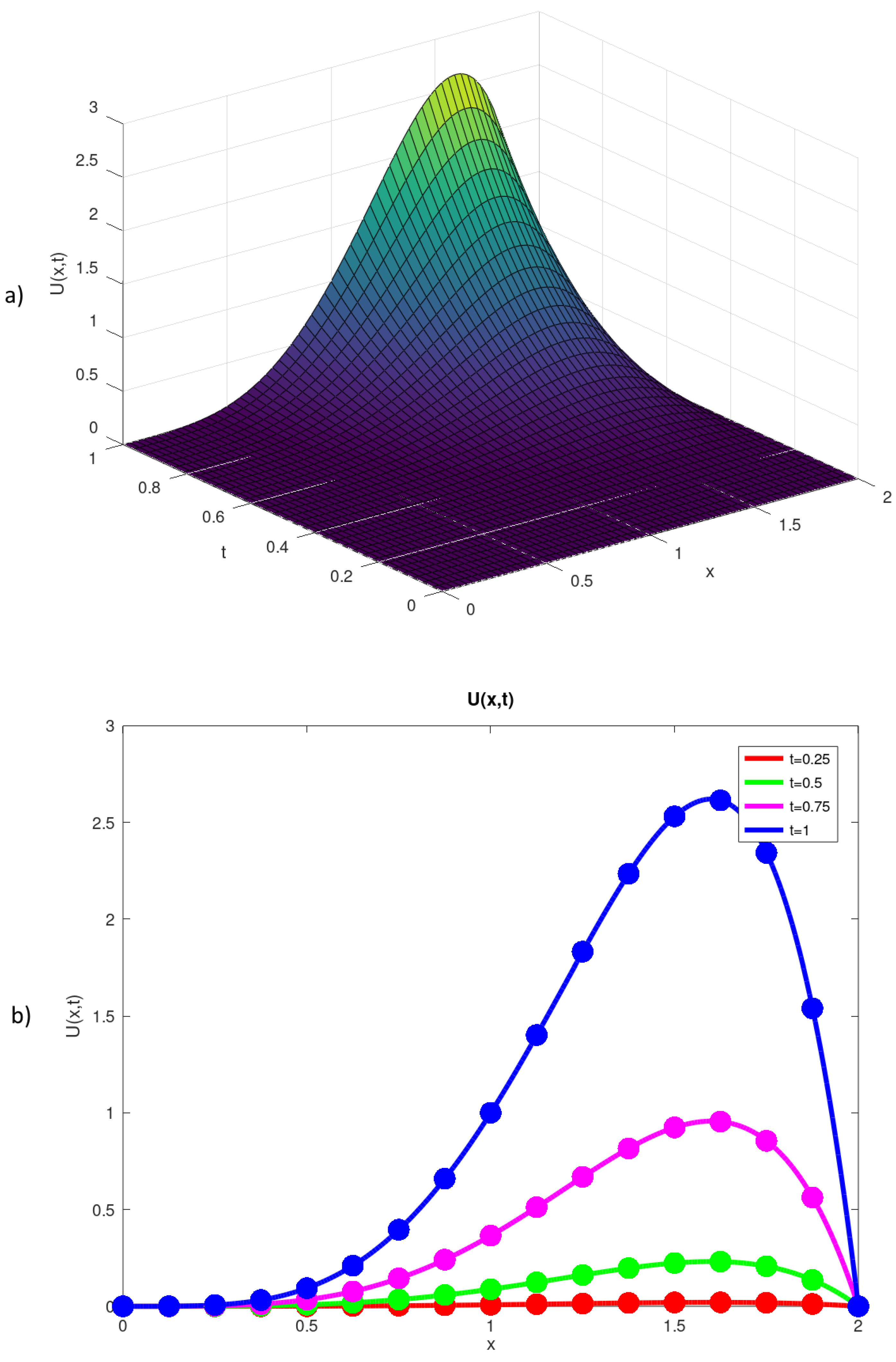
Figure 1 shows the approximate solution for Problem 1 obtained by the Thomas algorithm.

Table 1. Results of experiments for Problem 1.

Method	${\mathit{T}}_1$ [s]	${\mathit{T}}_8$ [s]	${\mathit{S}}_8$	K	${\mathit{K}}_{\mathit{n}}$	$\mathit{\delta }$
GS	271	255	1.06	$102.7·{10}^6$	6300	$1·{10}^{-3}$
SOR	132	74	1.78	$13.3·{10}^6$	800	$1·{10}^{-3}$
AOR	121	58	2.08	$6.3·{10}^6$	400	$1·{10}^{-3}$
Thomas Algorithm	8	2.3	3.5			$2.4·{10}^{-7}$
Parallel Sweep Method	8	2.5	3.2			$2.4·{10}^{-7}$

presents the results of numerical experiments. It contains the computing times of solving the Problem 1 by five methods described above. $T_1$ is the computing time by a single OpenMP thread, i.e., of the serial program implementing the given method. $T_8$ is the time by a parallel program for the same method run by 8 threads. To assess the efficiency of the parallel implementation, the speedup coefficient $S_L=T_1/T_L$ is presented, where L is the number of threads. The table also contains the total number K of iterations required to solve the problem by the iterative methods, as well as, the average number $K_n$ of iterations at a single time level. The last column presents the error $\delta ={∥\tilde{U}-U∥}_{\infty }$ of the solution obtained by a given method.

4.3.2. Problem 2

This test problem is based on the equation [36]

$$\frac{{\partial }^{\alpha }U(x,t)}{\partial t^{\alpha }}=\frac{{\partial }^{2}U(x,t)}{\partial x^2}+\frac{\Gamma (4+\alpha )}{6}{x}^2(2-x)t^3-4x^2(6-5x)t^{3+\alpha },$$

$$0<\alpha <1,0\le x\le 2,0\le t\le 1,$$

with the boundary conditions

$$U(0,t)=0,U(2,t)=0,$$

and the initial condition

$$U(x,0)=0.$$

The exact solution of this problem is given in work [37], it is

$$U(x,t)=x^4(2-x)t^{3+\alpha }.$$

The numerical experiments were performed for the order $\alpha =0.5$ on the grid $m=8192$, $N=8192$. The combination of parameters $\beta ,\gamma$ for the AOR method is $\beta =1.99,\gamma =1.9$.

Figure 2 shows the approximate solution for Problem 2 obtained by the Thomas algorithm.

Table 2. Results of experiments for Problem 2 with grid $m=8192,N=8192$.

Method	${\mathit{T}}_1$ [s]	${\mathit{T}}_2$ [s]	${\mathit{T}}_4$ [s]	${\mathit{T}}_8$ [s]	K	${\mathit{K}}_{\mathit{n}}$	$\mathit{\delta }$
AOR	144	117	96	92	$3.3·{10}^6$	400	$1·{10}^{-3}$
Thomas	89	64	49	47			$1·{10}^{-6}$
Parallel Sweep	89	64	49	47			$1·{10}^{-6}$

presents the results of numerical experiments for Problem 2 on the grid $m=8192,N=8192$.

For the next experiments, we use the large spatial grid $m=32\times 2^{20}$ for the same problem. The time grid in this experiment is just $N=64$. Thus, the program requires about 20 GB of memory out of 32 GB available on the PC used in tests.

Table 3. Results of experiments for Problem 2 using the full memory approach with grid $m=32\times 2^{20},N=64$.

Method and Subroutine	${\mathit{T}}_1$ [s]	${\mathit{T}}_2$ [s]	${\mathit{T}}_4$ [s]	${\mathit{T}}_8$ [s]	$\mathit{\delta }$
Thomas Algorithm					$0.5·{10}^{-2}$
(full memory)
Total	39.5	29.3	25.2	24
Right-hand parts	28	17.8	13.7	12.5
SLAE solver	11.5	11.5	11.5	11.5
Parallel Sweep Method					$0.8·{10}^{-2}$
(full memory)
Total	40.3	27.5	19.1	17.9
Right-hand parts	28	17.8	13.7	12.5
SLAE solver	12.3	9.3	5.4	5.4

and

Table 4. Results of experiments for Problem 2 using the logarithmic memory approach with grid $m=32\times 2^{20},N=64$.

Method and Subroutine	${\mathit{T}}_1$ [s]	${\mathit{T}}_2$ [s]	${\mathit{T}}_4$ [s]	${\mathit{T}}_8$ [s]	$\mathit{\delta }$
Thomas Algorithm					$0.5·{10}^{-2}$
(logarithmic memory)
Total	18.2	16.3	15.9	15.5
Right-hand parts	6.7	4.8	4.4	4
SLAE solver	11.5	11.5	11.5	11.5
Parallel Sweep Method					$1.5·{10}^{-2}$
(logarithmic memory)
Total	19	14.1	9.8	9.4
Right-hand parts	6.7	4.8	4.4	4
SLAE solver	12.3	9.3	5.4	5.4

present the results of numerical experiments for Problem 2 on this grid using the full memory (7) and logarithmic memory (21) approaches for computing the right-hand parts respectively. It also contains the execution times for separate subroutines of the parallel program obtained by profiling with the Intel VTune Profiler.

5. Discussion

The experiments show that for both problems, the iterative AOR method is clearly inferior to the much simpler direct methods, such as Thomas algorithm and parallel sweep method, in terms of both accuracy and computing time. For Problem 1, the AOR method with tuned parameters requires less iterations and shorter computing time that the Gauss-Seidel and SOR methods. But its computing time is still 15 to 25 times lower than the direct methods.

For coarser spatial grids, such as $m=256$ for Problem 1 and $m=8192$ for Problem 2, the parallel sweep method is slightly slower than the serial Thomas algorithm. This is caused by too much parallel overhead (time required for synchronizing the threads) for the small sizes of the SLAE. The results are more indicative for the large spatial grid $m=32\times 2^{20}$ (roughly 32 millions) in the last experiment. Here, the parallel sweep algorithm for solving the SLAE shows better time than the classic serial Thomas algorithm.

We also note that the percentage of computing the right-hand parts for each time step is up to two times larger than for solving the SLAE when we use the full memory approach (see Table 3). The computation complexity of the right-hand parts computing is quadratic, while direct methods for SLAE are linear. Using the logarithmic memory approach (see Table 4) reduces the time of computing the right-hand parts 3 to 4 times. Total computing time reduces up to twofold. The error of the solution remain of the same order than for the full memory.

Now, the SLAE solver takes more time than right-hand computation. This makes the effect of using the parallel solver more prominent. The parallel implementation on the basis of the parallel sweep method reduces the total computing time from 19 to 9.4 s. In contrast, the implementation which uses the classic serial Thomas algorithm reduces the computing time from 18 to 15.5 s. Thus, the parallel implementations run on 8 threads, gives the computing times of 15.5 and 9.4 s for the classic Thomas algorithms and the parallel sweep method, respectively, a speedup of 1.65 times.

Let us investigate the performance of the procedure of computing the right-hand parts deeper.

Table 5. Memory bandwidth utilization for computing the right-hand parts.

Number of Threads	DRAM Bandwidth Utilization [GB/s]
1	32
2	50
4	55
8	56
Maximum bandwidth	57

presents the memory bandwidth utilization for the parallel implementation of this procedure (for the full memory approach) for various number of the OpenMP threads measured by the Intel VTune Profiler for the grid size $m=8192,N=8192$.

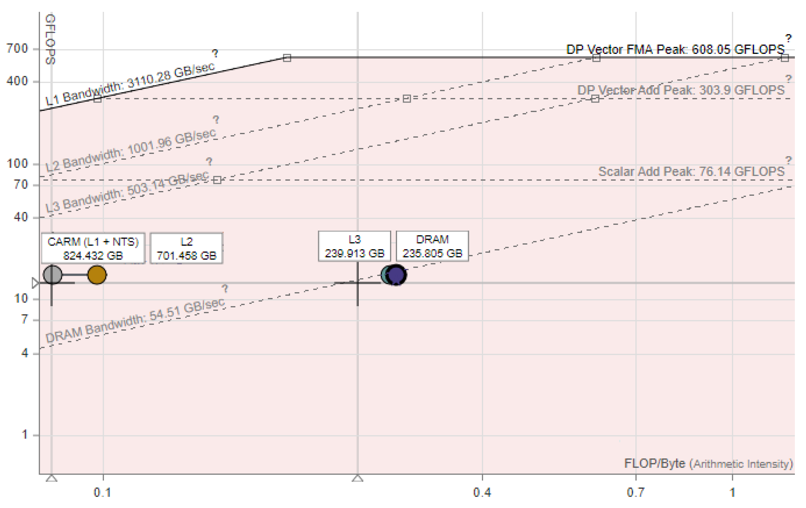
The table shows that even two threads saturate the memory bandwidth and further increase of the number of the threads produces miniscule improvement. This is confirmed by the results in Table 2, Table 3 and Table 4. The largest speedup is about 2 times, regardless of using the full or logarithmic memory. This is caused by the fact that the calculating the right-hand parts by Formulas (7) and (21) has low arithmetical intensity. Essentially, we perform one multiplication and one addition per 3 numbers read from memory. The roofline analysis by the Intel Advisor [38] confirms that this implementation is memory bound (see Figure 3).

There are several ways to get around this problem. One way is to use the hardware with higher memory bandwidth. Modern GPUs’ memory bandwidth is dozens of times higher than CPUs. For example, the NVIDIA RTX 3080 has memory bandwidth of 760 GB/s in comparison with the Intel i7-10700k with DDR4-4133 used in our experiments, which has 57 GB/s (with a comparable performance in the double precision arithmetic of about 450–500 GFLOPS).

The computing cluster systems with distributed memory allow the effective summation of the memory bandwidthes of the individual nodes. It also allows one to solve much larger problems when the total data would not fit into a memory of a single node. This makes the parallel sweep algorithm more viable for such systems.

The other way is to increase the arithmetic intensity and efficiency of memory access. Reusing the data in caches or shared memory can significantly improve the performance. Several methods for optimizing the computational procedures for fractional derivatives are proposed in works [39,40]. An algorithm for automatical optimization of the similar procedure of the matrix-vector multiplication for a multicore processor is presented in work [41].

In future, the Authors plan to develop the efficient numerical algorithms for the forward and inverse 2D and 3D problems for TFDEs. This would require a larger amount of computations, as well as, larger memory requirements. To obtain more efficient parallelization, various techniques may be implemented, such as using red-black partitioning, conjugate gradient type methods, preconditioning, higher-order schemes, etc. One of the promising ways to solve large time-fractional problems is the Parareal method [42]. Currently, it is widely used for numerical solving the initial boundary problems for classical differential equations with integer orders. Its main idea is the time domain decomposition using two grids (a coarse one and a fine one). The coarse grid is used to construct the initial approximations for the subtasks solved on a fine grid and for correcting the solution of the subtasks. The subtasks on a fine grid may be solved independently for each time subinterval. This allows one to implement the efficient parallel algorithms for various high-performance architectures.

6. Conclusions

In this work, the parallel algorithms for solving the initial boundary problem for the time-fractional diffusion equation are constructed. The algorithms are based on the finite-difference scheme for approximating the differential equation and the Thomas algorithm, parallel sweep algorithm, and accelerated over-relaxation method for solving the systems of linear algebraic equations. The algorithms are implemented for the multicore processors using the OpenMP technology. The numerical experiments were performed to investigate the efficiency of the developed parallel algorithms. The Thomas algorithm and parallel sweep algorithm reduce the total computing time for solving the example problems up to 25 times in comparison with the over-relaxation method and provides better accuracy. For the large spatial grids, using the parallel sweep method speed up the computations up to 2 times on the 8-core CPU in comparison with the classic serial Thomas algorithm. In future, the Authors plan to implement more elaborate algorithms to circumvent the limits of memory bandwidth. This would allow one to solve the larger problems.

References

- Kilbas, A.A.; Srivastava, H.M.; Trujillo, J.J. Theory and Applications of Fractional Differential Equations; Elsevier: Amsterdam, The Netherlands, 2006; Volume 204. [Google Scholar]
- Cui, M. Convergence analysis of high-order compact alternating direction implicit schemes for the two-dimensional time fractional diffusion equation. Numer. Algorithms 2013, 62, 383–409. [Google Scholar] [CrossRef]
- Jin, B.; Rundell, W. A tutorial on inverse problems for anomalous diffusion processes. Inverse Probl. 2015, 31, 035003. [Google Scholar] [CrossRef] [Green Version]
- Machado, J.T.; Galhano, A.; Trujillo, J. Science metrics on fractional calculus development since 1966. Fract. Calc. Appl. Anal. 2013, 16, 479–500. [Google Scholar] [CrossRef] [Green Version]
- Sultanov, M.A.; Durdiev, D.K.; Rahmonov, A.A. Construction of an Explicit Solution of a Time-Fractional Multidimensional Differential Equation. Mathematics 2021, 9, 2052. [Google Scholar] [CrossRef]
- Scher, H.; Montroll, E.W. Anomalous transit-time dispersion in amorphous solids. Phys. Rev. B 1975, 12, 2455–2477. [Google Scholar] [CrossRef]
- Kou, S.C. Stochastic modeling in nanoscale biophysics: Subdiffusion within proteins. Ann. Appl. Stat. 2008, 2, 501–535. [Google Scholar] [CrossRef]
- Metzler, R.; Jeon, J.H.; Cherstvy, A.G.; Barkai, E. Anomalous diffusion models and their properties: Non-stationarity, non-ergodicity, and ageing at the centenary of single particle tracking. Phys. Chem. Chem. Phys. 2014, 16, 24128–24164. [Google Scholar] [CrossRef] [Green Version]
- Diethelm, K.; Ford, N.; Freed, A.; Luchko, Y. Algorithms for the fractional calculus: A selection of numerical methods. Comput. Methods Appl. Mech. Eng. 2005, 194, 743–773. [Google Scholar] [CrossRef] [Green Version]
- Baleanu, D.; Diethelm, K.; Scalas, E.; Trujillo, J.J. Fractional Calculus: Models and Numerical Methods; World Scientific: Singapore, 2012; Volume 3. [Google Scholar]
- Li, C.; Zeng, F. Numerical Methods for Fractional Calculus; Chapman and Hall/CRC: London, UK, 2019. [Google Scholar]
- Gong, C.; Bao, W.; Tang, G.; Jiang, Y.; Liu, J. A parallel algorithm for the two-dimensional time fractional diffusion equation with implicit difference method. Sci. World J. 2014, 2014, 219580. [Google Scholar] [CrossRef]
- Akimova, E.N.; Martyshko, P.S.; Misilov, V.E.; Kosivets, R.A. An Efficient Numerical Technique for Solving the Inverse Gravity Problem of Finding a Lateral Density. Appl. Math. Inf. Sci. 2016, 10, 1681–1688. [Google Scholar] [CrossRef]
- Akimova, E.N.; Misilov, V.E.; Tretyakov, A.I. Optimized Algorithms for Solving Structural Inverse Gravimetry and Magnetometry Problems on GPUs. In Communication in Computer and Information Sciences; Springer International Publishing: Cham, Switzerland, 2017; pp. 144–155. [Google Scholar] [CrossRef]
- Akimova, E.N.; Filimonov, M.Y.; Misilov, V.E.; Vaganova, N.A. Simulation of thermal processes in permafrost: Parallel implementation on multicore CPU. In Proceedings of the 4th International Workshop on Radio Electronics and Information Technologies (REIT-Autumn 2018), Yekaterinburg, Russia, 16 November 2018; Volume 2274, pp. 1–9. Available online: http://ceur-ws.org/Vol-2274/paper-01.pdf (accessed on 1 December 2021).
- Akimova, E.N.; Misilov, V.E.; Sultanov, M.A. Parallel Implementation of the Conjugate Gradient Method for Solving the Inverse Gravimetry Problem on GPU. In Proceedings of the 18th International Conference on Geoinformatics—Theoretical and Applied Aspects, Kyiv, Ukraine, 13–16 May 2019; European Association of Geoscientists and Engineers: Houten, The Netherlands, 2019; pp. 1–5. [Google Scholar] [CrossRef]
- Akimova, E.N.; Misilov, V.E.; Sultanov, M.A. Regularized gradient algorithms for solving the nonlinear gravimetry problem for the multilayered medium. Math. Methods Appl. Sci. 2020, 11, 21. [Google Scholar] [CrossRef]
- Li, X.; Su, Y. A parallel in time/spectral collocation combined with finite difference method for the time fractional differential equations. J. Algorithms Comput. Technol. 2021, 15, 17483026211008409. [Google Scholar] [CrossRef]
- De Luca, P.; Galletti, A.; Ghehsareh, H.; Marcellino, L.; Raei, M. A GPU-CUDA framework for solving a two-dimensional inverse anomalous diffusion problem. Parallel Comput. Technol. Trends 2020, 36, 311. [Google Scholar]
- Yang, X.; Wu, L. A New Kind of Parallel Natural Difference Method for Multi-Term Time Fractional Diffusion Model. Mathematics 2020, 8, 596. [Google Scholar] [CrossRef] [Green Version]
- Wang, Q.; Liu, J.; Gong, C.; Tang, X.; Fu, G.; Xing, Z. An efficient parallel algorithm for Caputo fractional reaction-diffusion equation with implicit finite-difference method. Adv. Differ. Equ. 2016, 2016, 207. [Google Scholar] [CrossRef] [Green Version]
- Alimbekova, N.; Berdyshev, A.; Baigereyev, D. Parallel Implementation of the Algorithm for Solving a Partial Differential Equation with a Fractional Derivative in the Sense of Riemann-Liouville. In Proceedings of the 2021 IEEE International Conference on Smart Information Systems and Technologies (SIST), Nur-Sultan, Kazakhstan, 28–30 April 2021; pp. 1–6. [Google Scholar] [CrossRef]
- Sunarto, A.; Agarwal, P.; Sulaiman, J.; Chew, J.V.L.; Aruchunan, E. Iterative method for solving one-dimensional fractional mathematical physics model via quarter-sweep and PAOR. Adv. Differ. Equ. 2021, 2021, 147. [Google Scholar] [CrossRef]
- Zhang, Y. A finite difference method for fractional partial differential equation. Appl. Math. Comput. 2009, 215, 524–529. [Google Scholar] [CrossRef]
- Sunarto, A.; Sulaiman, J.; Saudi, A. Implicit finite difference solution for time-fractional diffusion equations using AOR method. In Proceedings of the 2014 International Conference on Science & Engineering in Mathematics, Chemistry and Physics (ScieTech 2014), Jakarta, Indonesia, 13–14 January 2014; Journal of Physics: Conference Series. IOP Publishing: Bristol, UK, 2014; Volume 495, p. 012032. [Google Scholar] [CrossRef] [Green Version]
- Samarskii, A.A.; Nikolaev, E.S. Numerical Methods for Grid Equations, Volume I: Direct Methods; Birkhäuser: Basel, Switzerland, 1989. [Google Scholar] [CrossRef]
- Stone, H.S. An Efficient Parallel Algorithm for the Solution of a Tridiagonal Linear System of Equations. J. ACM 1973, 20, 27–38. [Google Scholar] [CrossRef]
- Yanenko, N.; Konovalov, A.; Bugrov, A.; Shustov, G. Organization of Parallel Computing and the Thomas Algorithm Parallelization (in Russian). Numer. Methods Contin. Mech. (Comput. Cent. Sib. Branch USSR Acad. Sci. Novosib. 1978) 1978, 9, 139–146. [Google Scholar]
- Akimova, E.N. Parallel Algorithms for Solving the Gravimetry, Magnetometry, and Elastisity Problems on Multiprocessor Systems with Distributed Memory (in Russian). Thesis for the Degree of Doctor of Physical and Mathematical Sciences, Institute of Mathematics and Mechanics, Ural Branch of Russian Academy of Sciences, Ekaterinburg, Russia, 2009; 255p. Available online: https://www.dissercat.com/content/parallelnye-algoritmy-resheniya-zadach-gravi-magnitometrii-i-uprugosti-na-mnogoprotsessornyk (accessed on 1 December 2021).
- Hadjidimos, A. Accelerated overrelaxation method. Math. Comput. 1978, 32, 149–157. [Google Scholar] [CrossRef]
- Hughes-Hallett, A. The convergence of accelerated overrelaxation iterations. Math. Comput. 1986, 47, 219–223. [Google Scholar] [CrossRef] [Green Version]
- Yeyios, A. A necessary condition for the convergence of the accelerated overrelaxation (AOR) method. J. Comput. Appl. Math. 1989, 26, 371–373. [Google Scholar] [CrossRef] [Green Version]
- Chapman, B.; Jost, G.; Van Der Pas, R. Using OpenMP: Portable Shared Memory Parallel Programming; MIT Press: Cambridge, MA, USA; London, UK, 2007. [Google Scholar]
- Ford, N.J.; Simpson, A.C. The numerical solution of fractional differential equations: Speed versus accuracy. Numer. Algorithms 2001, 26, 333–346. [Google Scholar] [CrossRef]
- El-Sayed, A.; Gaber, M. The Adomian decomposition method for solving partial differential equations of fractal order in finite domains. Phys. Lett. A 2006, 359, 175–182. [Google Scholar] [CrossRef]
- Ferrás, L.L.; Ford, N.J.; Morgado, M.L.; Rebelo, M. A Numerical Method for the Solution of the Time-Fractional Diffusion Equation. In Computational Science and Its Applications—ICCSA 2014; Murgante, B., Misra, S., Rocha, A.M.A.C., Torre, C., Rocha, J.G., Falcão, M.I., Taniar, D., Apduhan, B.O., Gervasi, O., Eds.; Springer International Publishing: Cham, Switzerland, 2014; pp. 117–131. [Google Scholar]
- Murio, D.A. Implicit finite difference approximation for time fractional diffusion equations. Comput. Math. Appl. 2008, 56, 1138–1145. [Google Scholar] [CrossRef]
- Intel Corporation. Memory-Level Roofline Analysis in Intel Advisor. Available online: https://www.intel.com/content/www/us/en/developer/articles/technical/memory-level-roofline-model-with-advisor.html (accessed on 1 December 2021).
- Gong, C.; Bao, W.; Tang, G.; Yang, B.; Liu, J. An efficient parallel solution for Caputo fractional reaction–diffusion equation. J. Supercomput. 2014, 68, 1521–1537. [Google Scholar] [CrossRef]
- Liu, J.; Gong, C.; Bao, W.; Tang, G.; Jiang, Y. Solving the Caputo fractional reaction-diffusion equation on GPU. Discret. Dyn. Nat. Soc. 2014, 2014, 820162. [Google Scholar] [CrossRef]
- Gareev, R.A.; Akimova, E.N. Analytical modeling of matrix–vector multiplication on multicore processors. Math. Meth. Appl. Sci. 2021, 1–31. [Google Scholar] [CrossRef]
- Lions, J.L.; Maday, Y.; Turinici, G. Résolution d’EDP par un schéma en temps «pararéel». C. R. L’Académie Des Sci.-Ser. I-Math. 2001, 332, 661–668. [Google Scholar] [CrossRef] [Green Version]
Figure 1.
(a) Approximate solution of Problem 1 obtained by the Thomas algorithm; (b) exact (solid line) and approximate (dots) solutions at several time levels.
Figure 2.
(a) Approximate solution of Problem 2 obtained by the Thomas algorithm; (b) exact (solid line) and approximate (dots) solutions at several time levels.
Figure 3.
Roofline analysis for implementation of the right-hand parts computation procedure.