Enhanced Parallel Sine Cosine Algorithm for Constrained and Unconstrained Optimization

Abstract

The sine cosine algorithm’s main idea is the sine and cosine-based vacillation outwards or towards the best solution. The first main contribution of this paper proposes an enhanced version of the SCA algorithm called as ESCA algorithm. The supremacy of the proposed algorithm over a set of state-of-the-art algorithms in terms of solution accuracy and convergence speed will be demonstrated by experimental tests. When these algorithms are transferred to the business sector, they must meet time requirements dependent on the industrial process. If these temporal requirements are not met, an efficient solution is to speed them up by designing parallel algorithms. The second major contribution of this work is the design of several parallel algorithms for efficiently exploiting current multicore processor architectures. First, one-level synchronous and asynchronous parallel ESCA algorithms are designed. They have two favors; retain the proposed algorithm’s behavior and provide excellent parallel performance by combining coarse-grained parallelism with fine-grained parallelism. Moreover, the parallel scalability of the proposed algorithms is further improved by employing a two-level parallel strategy. Indeed, the experimental results suggest that the one-level parallel ESCA algorithms reduce the computing time, on average, by 87.4% and 90.8%, respectively, using 12 physical processing cores. The two-level parallel algorithms provide extra reductions of the computing time by 91.4%, 93.1%, and 94.5% with 16, 20, and 24 processing cores, including physical and logical cores. Comparison analysis is carried out on 30 unconstrained benchmark functions and three challenging engineering design problems. The experimental outcomes show that the proposed ESCA algorithm behaves outstandingly well in terms of exploration and exploitation behaviors, local optima avoidance, and convergence speed toward the optimum. The overall performance of the proposed algorithm is statistically validated using three non-parametric statistical tests, namely Friedman, Friedman aligned, and Quade tests.

1. Introduction

Metaheuristic optimization methods are widely used. Many of these algorithms are based on populations that evolve towards the optimal through an iterative process. In many cases, this iterative process is governed by rules based on natural phenomena, physical processes, or mathematical functions. Depending on both the evolutionary process of the populations (i.e., the algorithm used) and the characteristics of the function to be optimized (single-objective or multi-objective), the use of these methods may not be feasible, either because of the high computing cost or because of the poor quality of the result.

Some of the well-known metaheuristic optimization algorithms are based on natural phenomena. The most common algorithms are the ant colony optimization (ACO) algorithm [1], which imitates the foraging behavior of ant colonies; the evolutionary strategy (ES) algorithm [2], which is based on the processes of mutation and selection seen in evolution; the evolutionary programming [3] uses techniques for evolving programs based on the selection of individuals for reproduction (crossover) and mutation, as well the genetic programming [4]; the particle swarm optimization (PSO) algorithm [5], which is based on the social behavior of fish schooling or bird flocking; the shuffled frog leaping [6] algorithm, which imitates the collaborative behavior of frogs; and the artificial bee colony (ABC) algorithm [7], which was inspired by the foraging behavior of honey bees. Some algorithms are based on physical phenomena, for instance, the simulated annealing (SA) algorithm [8], which is based on the annealing process in metallurgy. Some algorithms based on human or non-human physiological processes have been proposed, such as genetic algorithms (GA) [9], which reflects the process of natural selection; the differential evolution (DE) [10,11,12] optimizes a problem by iteratively working to promote an agent concerning a given measure of quality; and the artificial immune algorithm (AIA) [13], which is based on the behavior of the human immune system. Some algorithms based on human social processes have also been proposed, such as the harmony search algorithm (HSA) [14] inspired by the process of musical performance. Finally, there are proposed algorithms based on mathematical processing, such as the SCA algorithm [15], which is based on the sine and cosine trigonometric functions.

Almost all of the algorithms mentioned require configuration parameters for an optimal optimization process. An incorrect setting of these parameters can cause either a poor quality solution or that the computational cost drastically increases as more generations are required to be processed. For example, ABC needs the number of bees and limits to be defined, HSA needs the harmony memory consideration rate, the number of improvisations, etc., to be adjusted. However, some of these algorithms do not require parameter tunings, such as teaching-learning based optimization algorithm (TLBO), Jaya, and SCA algorithms. The latter is employed in this paper.

The SCA algorithm has been proven to be efficient in various applications. In [16], SCA is used to train feed foreword neural network to breast cancer classification. Authors in [17] employ SCA algorithm to improve an adaptive fuzzy logic PID (proportional integral derivative) controller for the load frequency control of an autonomous power generation system. In addition, it is used to optimize the parameters of a fractional-order proportional integral differential controller for coordinated control of power consumption in heat pumps [18]. In [19], the unified power quality conditioner is formulated as a single objective problem optimized using SCA. The application spectrum of the SCA algorithm is too large, see for example [20,21,22,23,24,25,26,27]. However, its convergence speed is a bit slow, especially when considered multimodal objectives functions. Indeed, it maintains high global searchability even at the end of iterations. This paper aims to improve the SCA algorithm optimization behavior by intensifying the current solution’s refinement with a promising diversification level during the course of the algorithm, speeding it up both in terms of optimization and computational cost.

The major findings of the work are:

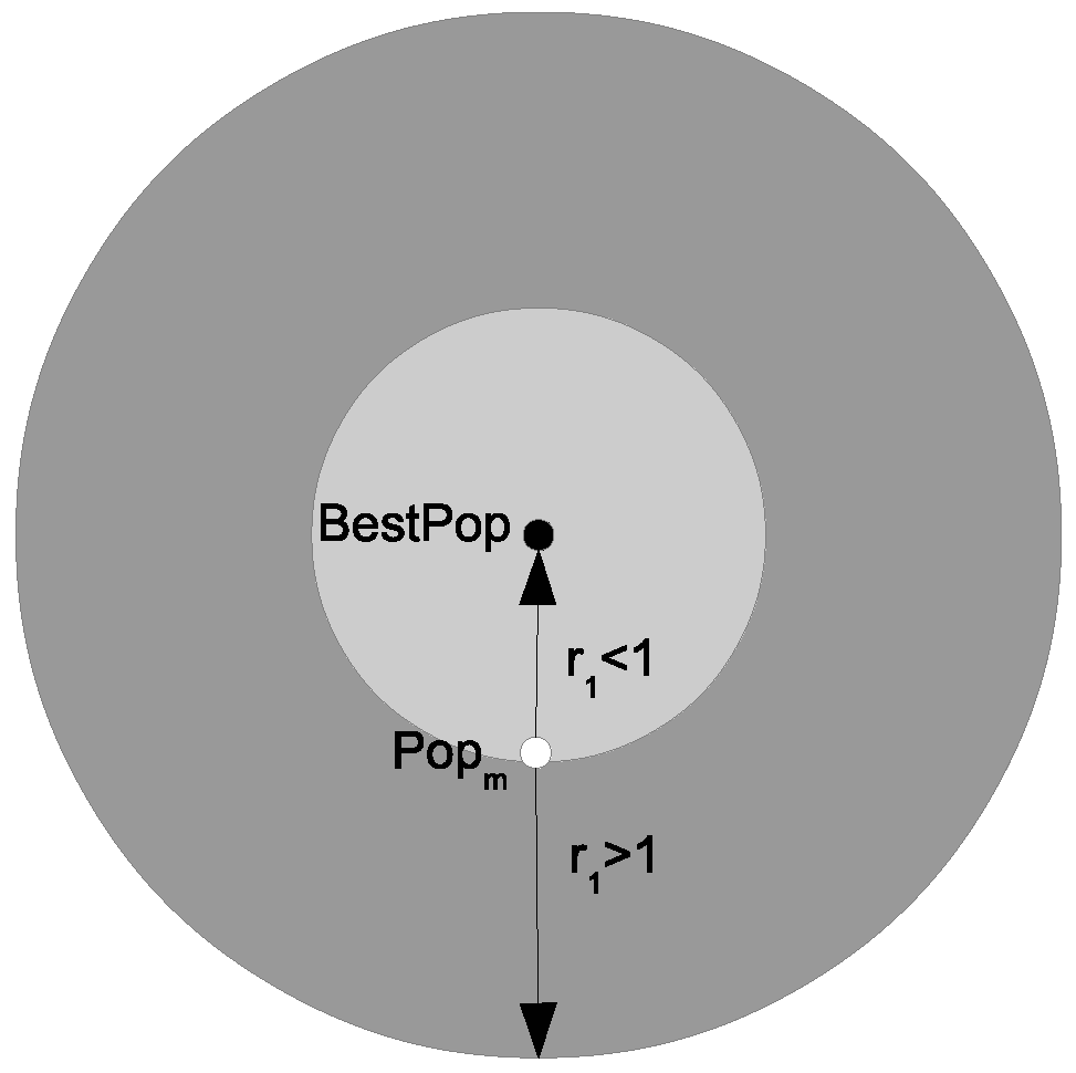
• A new optimization algorithm is proposed, dubbed the Enhanced Sine Cosine Algorithm (ESCA), which improves the SCA algorithm and offers better performance than a set of state-of-the-art algorithms. The outstanding optimization performance of the ESCA algorithm is based on the embedding of a best-guided approach along with the local search capability already existing in the SCA algorithm, leading to a decrease in the diversification behavior at the end of the iterations.
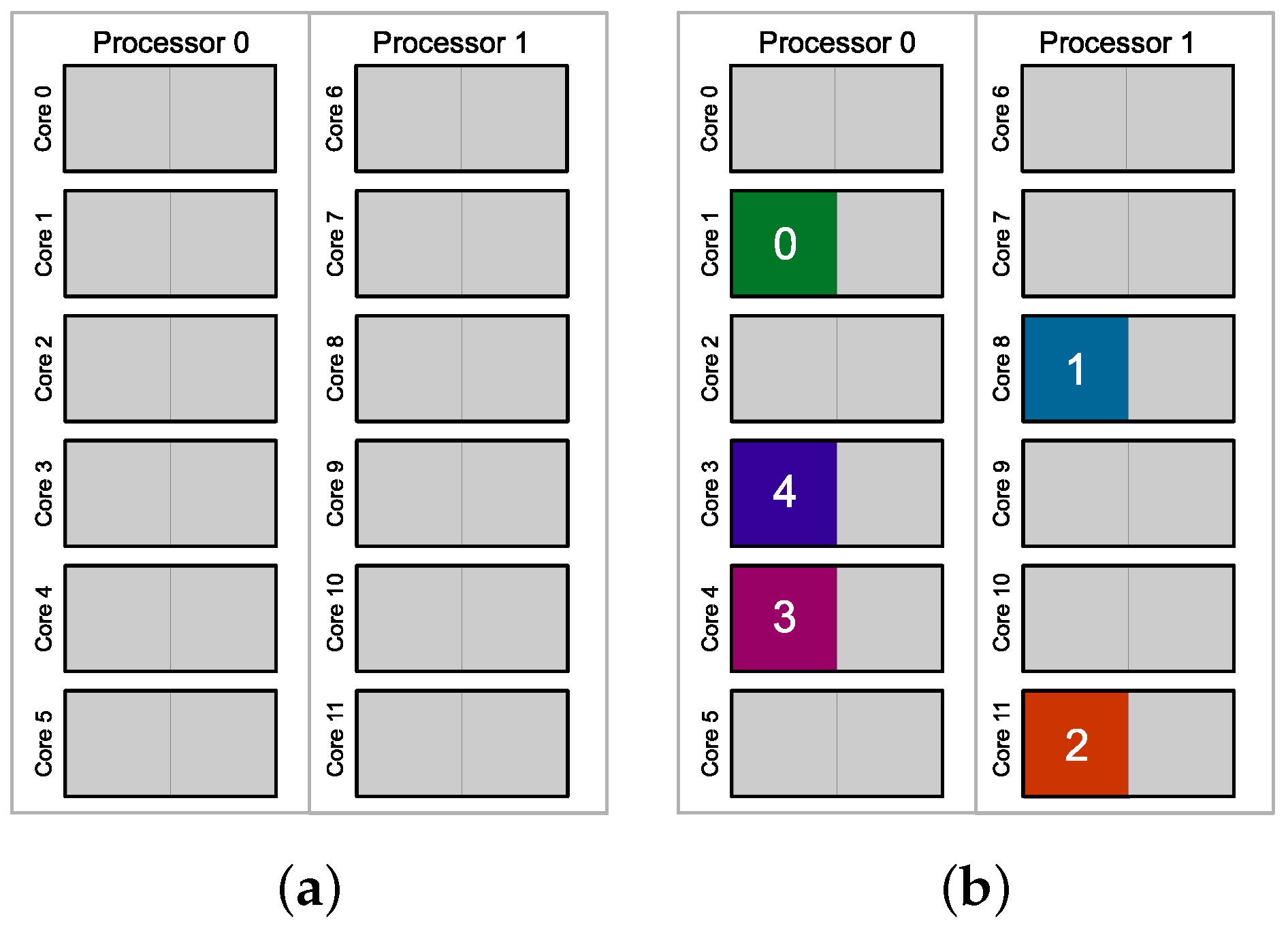
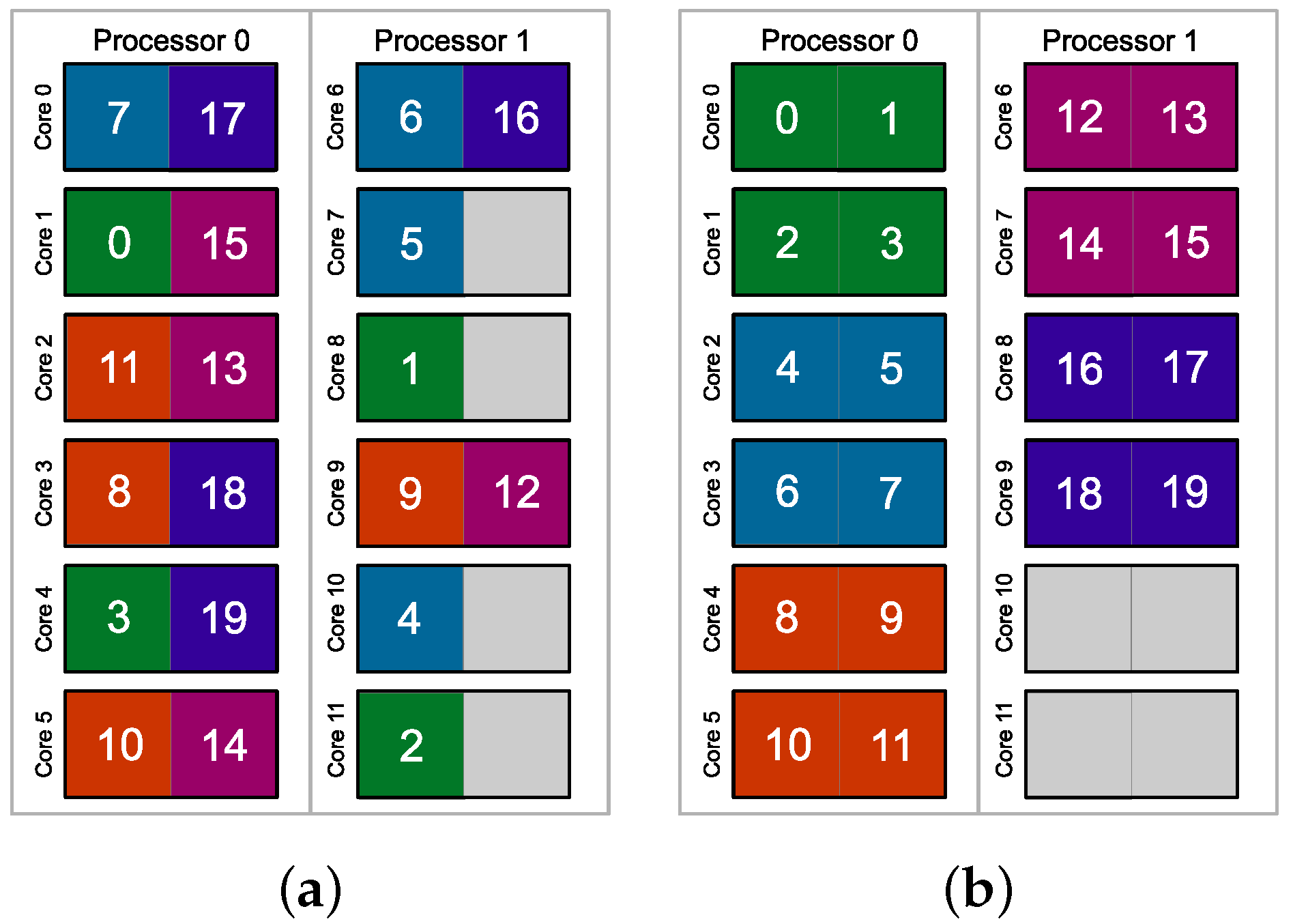
• To improve the computational performance of the proposed algorithm, synchronous and asynchronous parallel algorithms have been designed based on parallelization, initially at an outer, i.e., at a coarse-grained level. Since this level of parallelization is related to subpopulations, the number of subpopulations cannot increase indefinitely. These synchronous and asynchronous one-level parallel ESCA algorithms decrease the computing time by 87.4% and 90.8%, respectively, using 12 processing cores.
• To improve parallel scalability without harming the optimization performance and increasing the number of processes, two-level parallel algorithms have been designed. The parallel strategy includes two levels, namely the outer level and the internal level. The outer level corresponds to coarse-grained parallelization, while the internal level corresponds to fine-grained parallelization. Accordingly, the parallel scalability of the proposed algorithms is extremely improved. The experimental results show significant reductions in the computing time of 91.4%, 93.1%, and 94.5% with 16, 20, and 24 processes mapped on 12 physical cores. These time reductions correspond to speed-ups of $x12.5$, $x15.9$, and $x19.0$ with 16, 20, and 24 processes correctly mapped on 12 physical cores, i.e., using hyperthreading.

The rest of the paper is organized as follows. The preliminaries, including the sine cosine algorithm (SCA) and the related works, are provided in Section 2. The proposed enhanced SCA algorithm (ESCA) along with the proposed parallel algorithms based on multi-population are described in Section 3. Section 4 lists the benchmark functions and the engineering problems employed for testing the performance of the proposed algorithm. The experimental results of these algorithms are discussed in Section 5. Finally, Section 6 concludes the paper.

2. Related Work

The SCA algorithm, on which our ESCA proposal is based, is described in Section 2.1. Other proposals based on the SCA algorithm are listed and briefly described in Section 2.2.

2.1. Sine Cosine Algorithm

The SCA algorithm is an optimization algorithm based on an initial population that evolves in search of a function’s optimum, called a cost function. This evolution, i.e., the generation of consecutive new populations (the typical procedure of population-based algorithms), is mainly based on (1) and (2).

$$Po{p}_m^k=Po{p}_m^k+(r_1\ast sin\left(r_2^k\right)\left|r_3^k\ast BestPo{p}^k-Po{p}_m^k\right|)$$

(1)

$$Po{p}_m^k=Po{p}_m^k+(r_1\ast cos\left(r_2^k\right)\left|r_3^k\ast BestPo{p}^k-Po{p}_m^k\right|)$$

(2)

As can be seen, (1) and (2) differ only in the use of the mathematical functions sine or cosine. In these equations, it has been adopted that each population is composed of m individuals, each individual consists of k variables (this parameter depends on the cost function), and finally, the best current individual is denoted by $BestPop$. Each individual is generated based on both the current individual ($Po{p}_m$) and the current best individual ($BestPop$). However, the generation of each variable of each new individual is tuned by using three random values that define the magnitude of the sine or cosine range ($r_1$), the sine or cosine domain ($r_2^k$), and the magnitude of the contribution of the target ($BestPop$) in defining the new position of the solution ($r_3^k$).

In practice, the random numbers $r_1$ divide the search space into two sub-spaces based on the current individual and the best individual in the current population. Thus, if $r_1$ is greater than 1, the candidate solutions vacillate outwards the destination, else they fluctuate inwards the destination (see Figure 1).

Both exploration and exploitation phases of the SCA optimization algorithm depend on the capabilities provided by (1) and (2). This selection is decided at random with the same probability.

In heuristic optimization algorithms, which are iterative, the exploration phase is usually more decisive in the iterative procedure’s final phase. The SCA algorithm prioritizes the exploration phase as more iterations are performed through $r_1$ (see Equation (3)).

$$\begin{array}{c}\hfill r_1=iniValu{e}_{r_1}-curren{t}_{IT}\frac{iniValu{e}_{r_1}}{ma{x}_{ITs}}\end{array}$$

(3)

From an initial value ($iniValue\_r_1$), the value of $r_1$ decreases as the number of iterations performed increases, towards the $r_1$ minimum value when the last iteration is performed ($max\_ITs$). The initial value of $r_1$ is set to 2. The number of iterations to be performed ($max\_ITs$) is necessary for all population-based heuristic optimization algorithms. In practice, the value of $r_1$ modifies the range of values of the terms associated with the sine and cosine, from the original range $\left[-1,1\right]$ to the decreasing variable range, this variables range starts at $\left[-iniValue\_r_1,iniValue\_r_1\right]$. These variables’ contribution can be seen in Algorithm 1, which shows the steps of the SCA algorithm. The computed new individual is $newPo{p}_m$, the number of individuals in the population is $popSize$ and the number of cost function design variables is $numDesignVars$.

Algorithm 1 The SCA optimization algorithm.

1: Set $iniValu{e}_{r_1}=2$ 2: Set $ma{x}_{ITs}$ variable 3: Set population size (m - iterator for individuals) 4: Define function cost (k - iterator for design variables) 5: Generate initial population $Po{p}_0$ 6: for$iterator=1$ to $ma{x}_{ITs}$ do 7:    Search for the current $BestPop$ 8:    $r_1=iniValu{e}_{r_1}-iterator\frac{iniValu{e}_{r_1}}{ma{x}_{ITs}}$ 9:    for $m=0$ to $popSize$ do 10:      for $k=1$ to $numDesignVars$ do 11:         $r_2=2\ast \pi \ast ran{d}_{0..1}$ 12:         $r_3=2\ast ran{d}_{0..1}$ 13:         $r_4=ran{d}_{0..1}$ 14:         if $r_4<0.5$ then 15:           $newPo{p}_m^k=Po{p}_m^k+\left(r_1\ast sin\left(r_2\right)\left|r_3\ast BestPo{p}^k-Po{p}_m^k\right|\right)$ 16:         else 17:           $newPo{p}_m^k=Po{p}_m^k+\left(r_1\ast cos\left(r_2\right)\left|r_3\ast BestPo{p}^k-Po{p}_m^k\right|\right)$ 18:         end if 19:      end for 20:      $Po{p}_m=newPo{p}_m$ 21:    end for 22: end for 23: Search for the current $BestPop$

2.2. SCA-Based Proposals

Thanks to its simplicity, the SCA algorithm was widely adopted and refined in many research proposals. In [28], the authors proposed a modified SCA algorithm in which the linear transition rule was substituted by a non-linear transition to guarantee a better transition from exploration to exploitation. Second, the best guidance based on the elite candidate solution was entered in the SCA’s search equations. Third, to escape from local optimums, a mutation operator is utilized to produce a new position during the course of the algorithm. An improved alternative of SCA named HSCA for train multilayer perceptrons was reported in [29]. The HSCA adjusted the search mechanism of SCA by combining the leading guidance and the simulated quenching algorithm. In [30], a novel SCA based on orthogonal parallel information was presented. It is based on two approaches; multiple-orthogonal parallel information and experience-based opposition direction strategy. The former enabled the algorithm to save the solution diversification and search around promising regions simultaneously. The latter serves to guard the exploration ability of the SCA algorithm. Authors in [31] proposed an improved sine cosine algorithm (ISCA) for feature selection of text categorization. In addition to the position of the leading solution, the ISCA worked with random positions from the search space. That alteration of the solution’s position mitigated premature convergence and submitted adequate performance. Ref. [32] suggested an improved sine cosine algorithm in which a couple of new mechanisms are provided. One is the mixing of the exploitation abilities of crossover with the personal lead position of individual solutions. The other is the combination of self-learning and global search tools. Zhiliu et al. proposed a modified SCA algorithm based on vicinity search and greedy levy mutation [33]. It suggests three optimization tactics. Firstly, it mixed the exponential decreasing of conversion parameter and the linear decreasing of inertia weight, which yielded an equilibrium between the algorithm’s global and local search abilities. Secondly, to escape from local optimums, a random strategy for search agents around the best one is performed. Thirdly, the greedy Levy mutation strategy is adopted for the best individuals to intensify the algorithm’s local searchability. A hybrid modified SCA algorithm was studied in [34]. It was benefited from the ability of random populations through the Latin hypercube sampling method. Next, it was used for hybridization with the cuckoo search algorithm. The algorithm showed sufficient local and global search skills. Mohamed et al. presented an improved SCA algorithm based on opposition-based learning (OBL) [35]. Indeed, OBL is a machine learning approach usually utilized to boost the performance of metaheuristic optimization algorithms. It allowed better accuracy of the obtained solutions by promoting the exploration skills of the algorithm. Since OBL elected the leading element falling between a given solution and its opposite, better solutions are afforded accordingly. An enhanced SCA algorithm for feature selection was described in [36]. It embedded an elitism strategy and a new strategy of best solution updating, yielding better accuracy for pattern classification. In [37], the authors proposed an improved SCA algorithm for solving high-dimensional global optimization problems. The equation for renovating the position of the current solution and the linearly decreasing parameter were modified. In the former, inertia weight was introduced to speed up the convergence rate and avoid local optimums. The latter was replaced by a Gaussian function-based strategy that enabled a non-linear decrease of the parameter. Therefore, a promising exploration-exploitation balance was yielded. Other good attempts for improving the SCA algorithm can be found in [38,39,40,41,42]. In this subsection, some SCA-based algorithms have been reviewed. The motivation for the improvements in each of them is briefly described.

3. Proposed Work

In Section 3.1 our proposed optimization algorithm based on the SCA algorithm, called ESCA, is presented. Then in Section 3.2, the parallel algorithms developed to computationally accelerate the ESCA algorithm are presented.

3.1. Enhanced Sine Cosine Algorithm

The proposed enhanced sine cosine algorithm (ESCA) aims to improve the optimization behavior of the original SCA algorithm. For this purpose, we enhance the exploration and exploitation phases of the SCA optimization algorithm. Indeed, they depend on the capabilities provided by (1) and (2). These capacities are boosted by introducing a new alternative, defined by (4), to generate each new individual.

$$Po{p}_m^k=BestPo{p}^k+r_5^2(Po{p}_m^k-r_6\ast BestPo{p}^k)$$

(4)

When using (4), the new individual is generated based on the current individual and the distance between that individual and the best individual in the current population. Both the magnitude of the best individual and the magnitude of the distance are tuned using two random numbers, $r_5$ (which is squared) and $r_6$ respectively, as shown in (4).

The probability of using the sine-based equation, i.e., (1), remains at 50%. While the probability of using the cosine-based equation, i.e., (2), decreases to only 20%. The new equation uses neither sine nor cosine, and it has a 30% chance of being used. The proposed enhanced sine cosine algorithm (ESCA) is described in Algorithm 2.

Algorithm 2 Enhanced SCA (ESCA) optimization algorithm

1: Set $iniValu{e}_{r_1}=2$ 2: Set $ma{x}_{ITs}$ variable 3: Set population size (m - iterator for individuals) 4: Define function cost (k - iterator for design variables) 5: Generate initial population $Po{p}_0$ 6: for$iterator=1$ to $ma{x}_{ITs}$ do 7:    Search for the current $BestPop$ 8:    $r_1=iniValu{e}_{r_1}-iterator\frac{iniValu{e}_{r_1}}{ma{x}_{ITs}}$ 9:    for $m=0$ to $popSize$ do 10:      for $k=1$ to $numDesignVars$ do 11:         $r_2=2\ast \pi \ast ran{d}_{0..1}$ 12:         $r_3=2\ast ran{d}_{0..1}$ 13:         $r_4=ran{d}_{0..1}$ 14:         if $r_4<0.5$ then 15:           $newPo{p}_m^k=Po{p}_m^k+\left(r_1\ast sin\left(r_2\right)\left|r_3\ast BestPo{p}^k-Po{p}_m^k\right|\right)$ 16:         else if $r_4<0.7$ then 17:           $newPo{p}_m^k=Po{p}_m^k+\left(r_1\ast cos\left(r_2\right)\left|r_3\ast BestPo{p}^k-Po{p}_m^k\right|\right)$ 18:         else 19:           $r_5=ran{d}_{0..1}$ 20:           $r_6=round(1+ran{d}_{0..1})$ 21:           $newPo{p}_m^k=BestPo{p}^k+r_5^2(Po{p}_m^k-r_6\ast BestPo{p}^k)$ 22:         end if 23:      end for 24:      $Po{p}_m=newPo{p}_m$ 25:    end for 26: end for 27: Search for the current $BestPop$

In more detail, in the SCA algorithm two equations can be used to obtain a new individual, as can be seen in Algorithm 1 (lines 14–18), the first based on the sine function and the second based on the cosine function. Both equations have the same probability of being used, as can be seen in line 14 of Algorithm 1. In contrast, in our proposal up to three equations can be used, the first two coincide with the functions of the SCA algorithm, and the third is shown in Equation (4). The probability of using the equation based on the sine of the SCA algorithm remains unchanged.The probability of using the cosine-based equation of the SCA algorithm is reduced to 20%, while the new equation proposed in the ESCA algorithm has a 30% probability of being used, as can be seen in Algorithm 1 (lines 18–22).

To compare search agents’ behavior of the SCA and ESCA algorithms, the two-dimensional versions of the benchmark functions are solved by 30 search agents. The search maps of the search agents under 300 function evaluation times are shown in Figure 2, Figure 3 and Figure 4. Similarly, the distributions of all possible solutions over the entire search space are depicted in Figure 5, Figure 6 and Figure 7. These figures reveal that the ESCA algorithm searches around thoroughly narrow regions from the promising regions of the search space, which means reaching the optimum faster. In contrast, the SCA algorithm searches in dispersed areas of the entire space, so more time is required to attain the promising regions. In addition, the obtained solutions by the ESCA algorithm are almost distributed around the global optimum. This proves that it efficiently exploits the previous solutions to improve the current one and bypass significant jumps in the search space. The SCA algorithm’s weakness is that it favors exploration even at the end of iterations. An efficient optimization algorithm should hit an equilibrium of exploitation and exploration. Indeed, it should maintain a high level of diversification at the beginning and a lower one at its end to avoid falling on local optimums. Simultaneously, the algorithm refines the current solution progressively. Briefly, the algorithm should promote exploration in the beginning and exploitation at the end. In this context, the ESCA algorithm is guided by the current best solution (see Equation (4)) to converge toward the optimum and sustain a high level of intensification at the end of the algorithm. Accordingly, a better balance between local search and global search is guaranteed over the course of iterations.

3.2. Proposed Parallel Algorithms

Almost all newer computing platforms, regardless of their computing power, are parallel. The main trends to increase the platforms’ computing power are (i) increasing the number of processing units (physical cores and/or logical threads) and (ii) including hardware accelerators (GPUs, FPGAs, etc.). We propose parallel algorithms based on multicore platforms to efficiently use the computational resources available on shared memory parallel platforms.

First, two parallel coarse-grained algorithms based on multi-population are developed. Similar strategies applied to different heuristic optimization are presented in [43,44] and some other well-known algorithms. In both, the SCA and the proposed ESCA algorithms, only the population size and the stop criterion need to be established. Since the proposed parallel algorithms are based on multi-populations, the selected population size is that of the initial population, i.e., before it is partitioned. The stop criterion is the number of new generations to be computed. Note that the number of generations and the population’s size implicitly determine the number of cost function evaluations to be performed.

The initial population is divided into subpopulations of equal or similar size. The size of the subpopulations depends on the number of used processing units as shown in Algorithm 3 (line 4). If the size of the initial population is not divisible by the number of processing units, the sizes of some subpopulations are increased by one as exhibited in lines 5–9 of Algorithm 3.

Algorithm 3 Multi-population sizes computing

1: Initial population size: $popInitSize$ 2: Number of cores (or processes): $NoCs$ 3: Process ID: $idPr\in [0,NoCs-1]$ 4: $subpopSize=\frac{popInitSize}{NoCs}$ 5: if$(subpopSize\%NoCs)!=0$then 6:    if $idPr<(PopulationSize\%NoCs)$ then 7:      $subpopSize=subpopSize+1$ 8:    end if 9: end if

Once the size of the subpopulations is determined according to the size of the initial population and the number of processes, as can be seen in Algorithm 3, each subpopulation is processed by a single process. The required communications between these concurrent processes depend on the operating algorithm. The asynchronous approach reduces these communications with respect to the synchronous algorithm. Note that when hyperthreading is not used, each core runs only one process. In our case, hyperthreading is used when more than 12 processes are required.

As stated, the proposed parallel algorithms are suitable for shared memory platforms. In both algorithms, to efficiently exploit shared-memory platforms, private memory has been used preferably. The first proposed parallel algorithm, shown in Algorithm 4, is asynchronous, i.e., communications between processes are not needed. Algorithm 4 shows the parallel processing implemented in the asynchronous parallel method, i.e., the processing performed once each sequential thread has spawned the parallel region. A new subpopulation individual ($newS{P}_m$) is computed based on the current subpopulation individual ($S{P}_m$) and the best subpopulation individual ($subpopBest$).

It is worth mentioning that the concurrent processing shown in Algorithm 4 lacks synchronization points. This strategy allows having populations of significantly different sizes and leads to balancing the computing load through the number of generations processed by each thread and thus not degrading parallel efficiency.

Algorithm 5 presents the second parallel strategy in which the concurrent processes share data to obtain the best individual from the whole population, i.e., the best of all subpopulations. This process is done both at the beginning (line 7) and after computing each new generation by each parallel process (line 29). To ensure that all concurrent processes use the best individual from the whole population ($wholepopBest$) in each new generation, a synchronization point is needed after the critical section (line 35).

As shown in Algorithms 4 and 5, the population size assigned to each process depends on the size of the whole population ($popInitSize$) and the number of computing processes $NoCs$ (see Algorithm 3). That is, as the number of processes increases, the size of the subpopulations decreases. When tiny populations are used in population-based heuristic optimization algorithms, the optimization behavior can be significantly degraded. To further increase the number of processes and thus further reduce the computing time without drastically reducing the subpopulation sizes, we propose a two-level parallel algorithm. The parallel second level (fine-grained level) is applied to obtain a new generation of each subpopulation (see lines 10 and 26 of Algorithm 4).

Algorithm 4 Asynchronous parallel algorithm.

1: Allocate private memory for subpopulation: $S{P}_{[0,subpopSize]}$ 2: Allocate private memory for best individual: $subpopBest$ 3: Set $iniValu{e}_{r_1}=2$ 4: Generation counter: $genIt=0$ 5: Generate initial subpopulation $S{P}_0$ 6: while$genIt<numGenerations$do 7:    Search for the current subpop best $subpopBest$ 8:    $genIt=genIt+1$ 9:    $r_1=iniValu{e}_{r_1}-genIt\frac{iniValu{e}_{r_1}}{numGenerations}$ 10:    for $m=1$ to $subpopSize$ do 11:      for $k=1$ to $numDesignvars$ do 12:         $r_2=2\ast \pi \ast ran{d}_{0..1}$ 13:         $r_3=2\ast ran{d}_{0..1}$ 14:         $r_4=ran{d}_{0..1}$ 15:         if $r_4<0.5$ then 16:           $newS{P}_m^k=S{P}_m^k+\left(r_1\ast sin\left(r_2\right)\left|r_3\ast subpopBes{t}^k-S{P}_m^k\right|\right)$ 17:         else if $r_4<0.7$ then 18:           $newS{P}_m^k=S{P}_m^k+\left(r_1\ast cos\left(r_2\right)\left|r_3\ast subpopBes{t}^k-S{P}_m^k\right|\right)$ 19:         else 20:           $r_5=ran{d}_{0..1}$ 21:           $r_6=round(1+ran{d}_{0..1})$ 22:           $newS{P}_m^k=subpopBes{t}^k+r_5^2(S{P}_m^k-r_6\ast subpopBes{t}^k)$ 23:         end if 24:      end for 25:      $S{P}_m=newS{P}_m$ 26:    end for 27: end while

In the two-level algorithm the subpopulations are not calculated as a function of the total number of processes, since a single process will not process each subpopulation. The total number of processes in the two-level algorithm is equal to the number of subpopulations multiplied by the number of processes that will process each subpopulation. The number of subpopulations will be equal to the number of external processes ($NoCs$), while the number of processes that will process each subpopulation will be denoted by $inCs$. Therefore, the total number of processes equals to $NoCs\times inCs$.

Important modifications in Algorithm 4 are required that could degrade the parallel performance of the two-level parallel algorithm given in Algorithm 6. Since several threads will process each subpopulation, it must be stored in shared memory (line 1 of Algorithm 6), instead of being stored in private memory as in Algorithm 4. Moreover, before processing each subpopulation, the best individual must be available for all the processes involved in processing each subpopulation. This implies a synchronization point (line 9 of Algorithm 6) that determine the best individual. Thereafter each process checks if the current best individual stored in its private memory ($subpopBest$) should be updated.

Algorithm 5 Parallel algorithm with data sharing.

1: Shared memory: $wholepopBest$ 2: Allocate private memory for: $S{P}_{[0,subpopSize]}$ and $subpopBest$ 3: Set $iniValu{e}_{r_1}=2$ 4: Generation counter: $genIt=1$ 5: Generate initial subpopulation $S{P}_0$ 6: Search for the current subpopulation best $subpopBest$ 7: $wholepopBest=Bestof\left(subpopBes{t}_{NoCs}\right)$ 8: while$genIt<numGenerations$do 9:    $genIt=genIt+1$ 10:    $r_1=iniValu{e}_{r_1}-genIt\frac{iniValu{e}_{r_1}}{numGenerations}$ 11:    for $m=1$ to $subpopSize$ do 12:      for $k=1$ to $numDesignvars$ do 13:         $r_2=2\ast \pi \ast ran{d}_{0..1}$ 14:         $r_3=2\ast ran{d}_{0..1}$ 15:         $r_4=ran{d}_{0..1}$ 16:         if $r_4<0.5$ then 17:           $newS{P}_m^k=S{P}_m^k+\left(r_1\ast sin\left(r_2\right)\left|r_3\ast subpopBes{t}^k-S{P}_m^k\right|\right)$ 18:         else if $r_4<0.7$ then 19:           $newS{P}_m^k=S{P}_m^k+\left(r_1\ast cos\left(r_2\right)\left|r_3\ast subpopBes{t}^k-S{P}_m^k\right|\right)$ 20:         else 21:           $r_5=ran{d}_{0..1}$ 22:           $r_6=round(1+ran{d}_{0..1})$ 23:           $newS{P}_m^k=subpopBes{t}^k+r_5^2(S{P}_m^k-r_6\ast subpopBes{t}^k)$ 24:         end if 25:      end for 26:      $S{P}_m=newS{P}_m$ 27:    end for 28:    Search for the current subpopulation best $subpopBest$ 29:    CRITICAL parallel section: 30:      if $F_{eval}\left(subpopBest\right)<F_{eval}\left(wholepopBest\right)$ then 31:         $wholepopBest=subpopBest$ 32:      else 33:         $subpopBest=wholepopBest$ 34:      end if 35:    end CRITICAL 36: end while

Note that, in Algorithm 6 the total number of processes is increased from $NoCs$ to $NoCs\times inCs$, using the same subpopulation size. There are several options to implement the second level of parallelism (lines 13–29 of Algorithm 6), which will be discussed in Section 5.

Algorithm 6 Two-level parallel algorithm.

1: Allocate shared memory for $NoCs$ subpopulations: $S{P}_{[0,subpopSize]}$ 2: Total number of processes: $NoCs\times inCs$ processes. 3: Allocate private memory for best individual: $subpopBest$ 4: Set $iniValu{e}_{r_1}=2$ 5: Generation counter: $genIt=0$ 6: Generate initial subpopulation $S{P}_0$ 7: while$genIt<numGenerations$do 8:    Search for the current subpopulation best $subpopBest$ 9:    {Synchronization point} 10:    $genIt=genIt+1$ 11:    $r_1=iniValu{e}_{r_1}-genIt\frac{iniValu{e}_{r_1}}{numGenerations}$ 12:    {FOR processed in PARALLEL using $inCs$ processes} 13:    for $m=1$ to $subpopSize$ do 14:      for $k=1$ to $numDesignvars$ do 15:         $r_2=2\ast \pi \ast ran{d}_{0..1}$ 16:         $r_3=2\ast ran{d}_{0..1}$ 17:         $r_4=ran{d}_{0..1}$ 18:         if $r_4<0.5$ then 19:           $newS{P}_m^k=S{P}_m^k+\left(r_1\ast sin\left(r_2\right)\left|r_3\ast subpopBes{t}^k-S{P}_m^k\right|\right)$ 20:         else if $r_4<0.7$ then 21:           $newS{P}_m^k=S{P}_m^k+\left(r_1\ast cos\left(r_2\right)\left|r_3\ast subpopBes{t}^k-S{P}_m^k\right|\right)$ 22:         else 23:           $r_5=ran{d}_{0..1}$ 24:           $r_6=round(1+ran{d}_{0..1})$ 25:           $newS{P}_m^k=subpopBes{t}^k+r_5^2(S{P}_m^k-r_6\ast subpopBes{t}^k)$ 26:         end if 27:      end for 28:      $S{P}_m=newS{P}_m$ 29:    end for 30: end while

4. Benchmark Test

The benchamark test used in this work is composed of 30 well-known unconstrained functions shown in Section 4.1, and three constrained engineering design problems shown in Section 4.2.

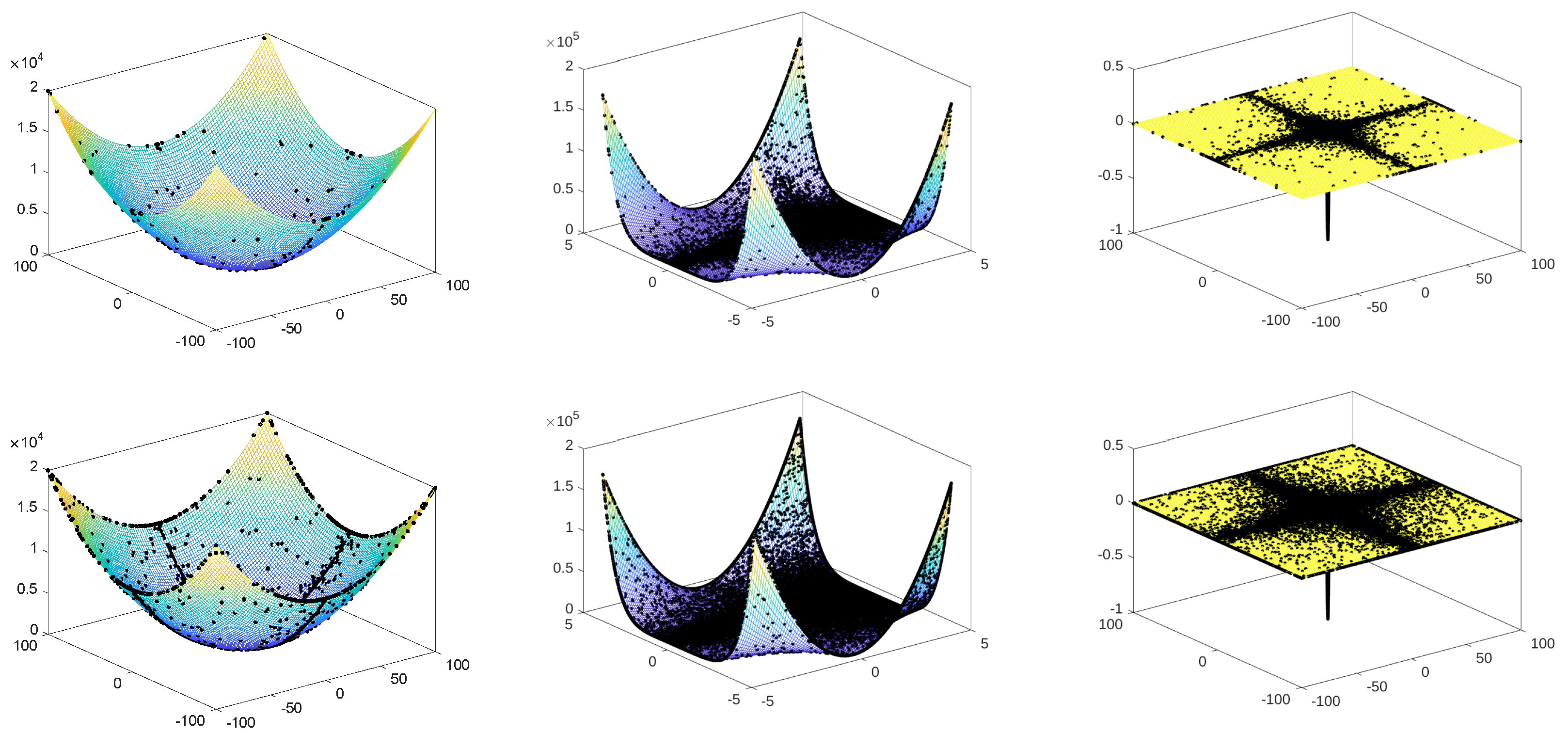
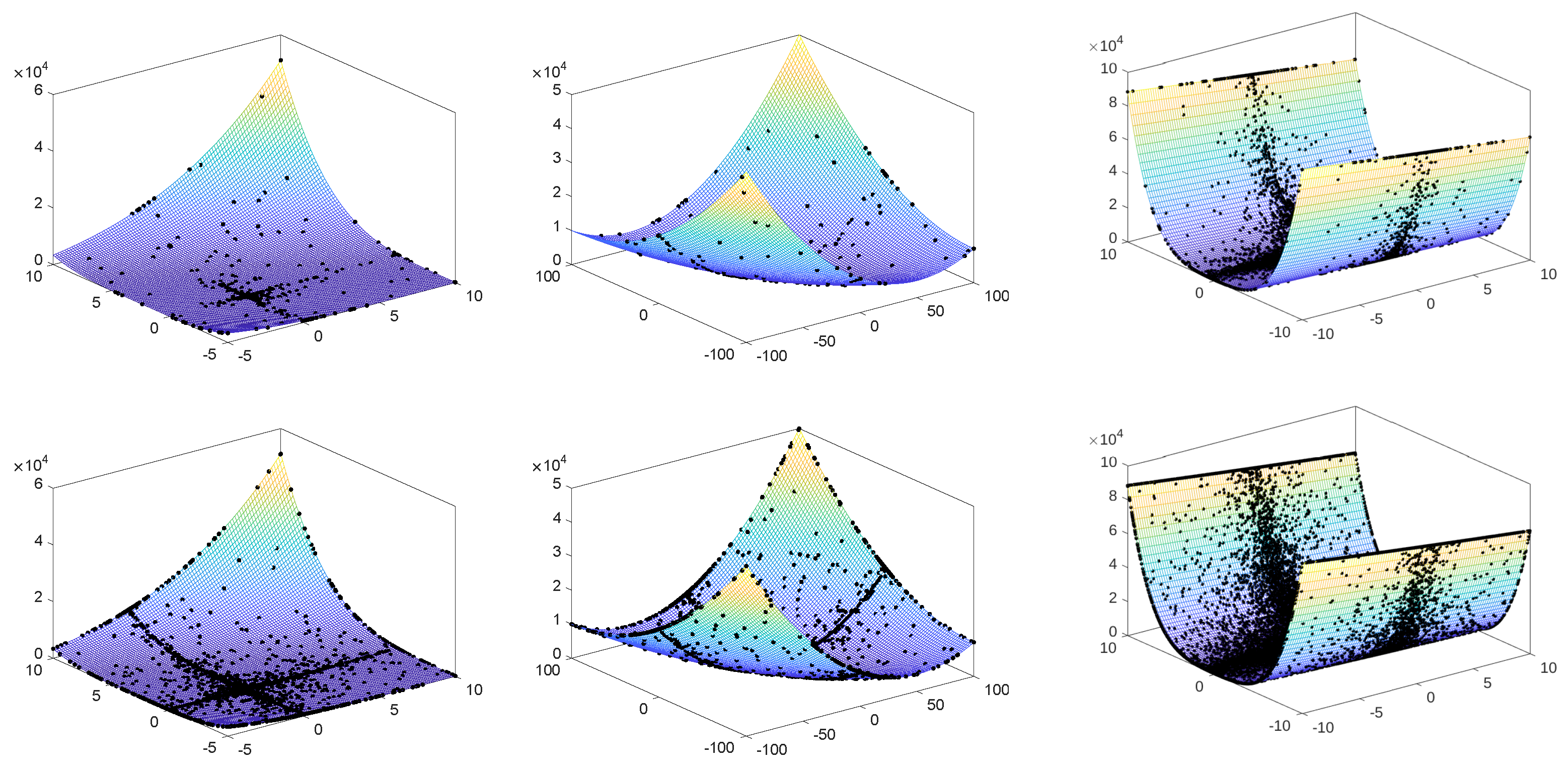
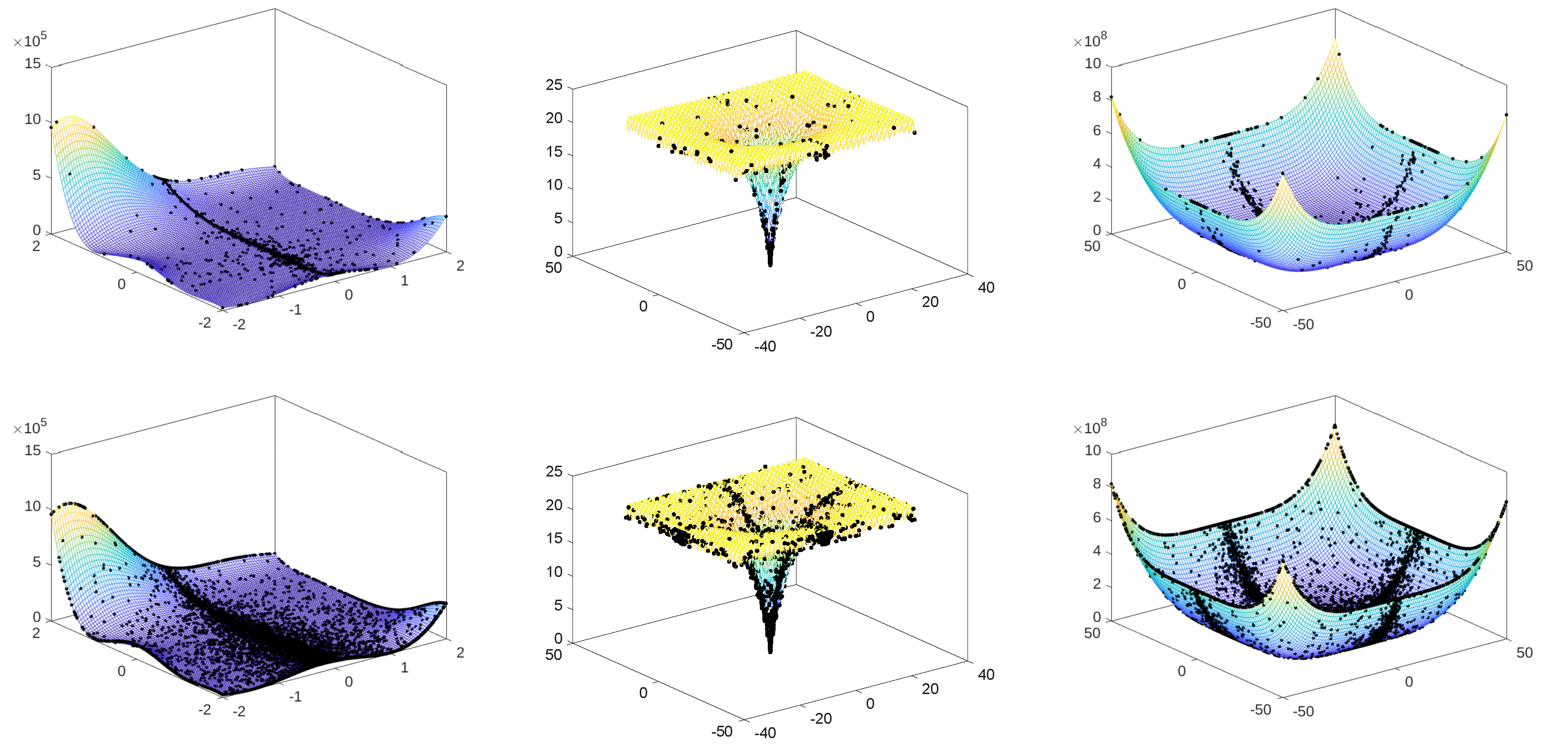
4.1. Benchmark Functions

A total of 30 well-known unconstrained functions used for the performance analysis are listed and described in

Table 1. Benchmark functions: dimensions and domain.

Id.	Name	Dim. (V)	Domain (Min, Max)
$f_1$	Sphere	30	$-100,100$
$f_2$	SumSquares	30	$-10,10$
$f_3$	Beale	2	$-4.5,4.5$
$f_4$	Easom	2	$-100,100$
$f_5$	Matyas	2	$-10,10$
$f_6$	Colville	4	$-10,10$
$f_7$	Trid 6	6	$-V^2,V^2$
$f_8$	Trid 10	10	$-V^2,V^2$
$f_9$	Zakharov	10	$-5,10$
$f_{10}$	Schwefel_1.2	30	$-100,100$
$f_{11}$	Rosenbrock	30	$-30,30$
$f_{12}$	Dixon-Price	5	$-10,10$
$f_{13}$	Foxholes	2	$-2^{16},2^{16}$
$f_{14}$	Branin	2	$x_1:-5,10$ $x_2:0,15$
$f_{15}$	Bohachevsky_1	2	$-100,100$
$f_{16}$	Booth	2	$-10,10$
$f_{17}$	Michalewicz_2	2	$0,\pi$
$f_{18}$	Michalewicz_5	5	$0,\pi$
$f_{19}$	Bohachevsky_2	2	$-100,100$
$f_{20}$	Bohachevsky_3	2	$-100,100$
$f_{21}$	GoldStein-Price	2	$-2,2$
$f_{22}$	Perm	4	$-V,V$
$f_{23}$	Hartman_3	3	$0,1$
$f_{24}$	Ackley	30	$-32,32$
$f_{25}$	Penalized_2	30	$-50,50$
$f_{26}$	Langermann_2	2	$0,10$
$f_{27}$	Langermann_5	5	$0,10$
$f_{28}$	Langermann_10	10	$0,10$
$f_{29}$	Fletcher-Powell_5	5	$x_i,{\alpha }_i:-\pi ,\pi$ $a_{ij},b_{ij}:-100,100$
$f_{30}$	Fletcher-Powell_10	10	$x_i,{\alpha }_i:-\pi ,\pi$ $a_{ij},b_{ij}:-100,100$

and

Table 2. Benchmark functions: Definitions.

Id.	Function
$f_1$	${\displaystyle f=\sum _{i=1}^V{x}_i^2}$
$f_2$	${\displaystyle f=\sum _{i=1}^{V}i{x}_i^2}$
$f_3$	$f={(1.5-x_1+x_1{x}_2)}^2+{(2.25-x_1+x_1{x}_2^2)}^2$ $+{(2.625-x_1+x_1{x}_2^3)}^2$
$f_4$	$f=-cos\left(x_1\right)cos\left(x_2\right)exp\left(-{(x_1-\pi )}^2-{(x_2-\pi )}^2\right)$
$f_5$	$f=0.26(x_1^2+x_2^2)-0.48x_1{x}_2$
$f_6$	$f=100{(x_1^2-x_2)}^2+{(x_1-1)}^2+{(x_3-1)}^2+90{(x_3^2-x_4)}^2$ $+10.1\left({(x_2-1)}^2+{(x_4-1)}^2\right)+19.8(x_2-1)(x_4-1)$
$f_7$	${\displaystyle f=\sum _{i=1}^V{(x_i-1)}^2-\sum _{i=2}^V{x}_i{x}_{i-1}}$
$f_8$
$f_9$	${\displaystyle f=\sum _{i=1}^V{x}_i^2+{\left({\displaystyle \sum _{i=1}^{V}0.5i{x}_i}\right)}^2+{\left({\displaystyle \sum _{i=1}^{V}0.5i{x}_i}\right)}^4}$
$f_{10}$	${\displaystyle f=\sum _{i=1}^V{\left({\displaystyle \sum _{j=1}^i{x}_j}\right)}^2}$
$f_{11}$	${\displaystyle f=\sum _{i=1}^{V-1}\left(100{(x_{i+1}-x_i^2)}^2+{(x_i-1)}^2\right)}$
$f_{12}$	${\displaystyle f={(x_1-1)}^2+\sum _{i=2}^{V}i{\left(2x_i^2-x_{i-1}\right)}^2}$
$f_{13}$	$f={\left[{\displaystyle \frac{1}{500}+\sum _{j=1}^{25}\frac{1}{{\displaystyle j+\sum _{i=1}^2{(x_i-a_{ij})}^6}}}\right]}^{-1}$
$f_{14}$	$f={\left(x_2-\frac{5.1}{4{\pi }^2}{x}_1^2+\frac{5}{\pi }{x}_1-6\right)}^2+10\left(1-\frac{1}{8\pi }\right)cos{x}_1+10$
$f_{15}$	$f=x_1^2+2x_2^2-0.3cos\left(3\pi x_1\right)-0.4cos\left(4\pi x_2\right)+0.7$
$f_{16}$	$f={(x_1-2x_2-7)}^2+{(2x_1+x_2-5)}^2$
$f_{17}$	${\displaystyle f=-\sum _{i=1}^{V}sin{x}_i{\left(sin\left(\frac{i{x}_i^2}{\pi }\right)\right)}^{20}}$
$f_{18}$
$f_{19}$	$f=x_1^2+2x_2^2-0.3cos\left(3\pi x_1\right)cos\left(4\pi x_2\right)+0.3$
$f_{20}$	$f=x_1^2+2x_2^2-0.3cos(3\pi x_1+4\pi x_2)+0.3$
$f_{21}$	$f=\left[1+{(x_1+x_2+1)}^2(19-14x_1+3x_1^2-14x_2+6x_1{x}_2+3x_2^2)\right]$ $\left[30+{(2x_1-3x_2)}^2(18-32x_1+12x_1^2+48x_2-36x_1{x}_2+27x_2^2)\right]$
$f_{22}$	${\displaystyle f=\sum _{j=1}^V{\left[{\displaystyle \sum _{i=1}^i(i^j+\beta )\left({\left(\frac{x_i}{i}\right)}^j-1\right)}\right]}^2}$
$f_{23}$	${\displaystyle f=-\sum _{i=1}^4{c}_{i}exp\left[{\displaystyle -\sum _{j=1}^3{a}_{ij}{(x_j-p_{ij})}^2}\right]}$
$f_{24}$	$f=-20exp\left(-0.2\sqrt{{\displaystyle \frac{1}{V}\sum _{i=1}^V{x}_i^2}}\right)-exp\left({\displaystyle \frac{1}{V}\sum _{i=1}^{V}cos\left(2\pi x_i\right)}\right)+20+e$
$f_{25}$	${\displaystyle f=0.1\{{sin}^2\left(3\pi x_1\right)+\sum _{i=1}^{V-1}{(x_i-1)}^2\left[1+{sin}^2\left(3\pi x_{i+1}\right)\right]+{(x_V-1)}^2\left[1+{sin}^2\left(2\pi x_V\right)\right]\}}$ ${\displaystyle +\sum _{i=1}^{V}u(x_i,5,100,4),}$ $u(x_i,a,k,m)=k{(x_i-a)}^m,x_i>a;0,-a\le x_i\le a;k{(-x_i-a)}^m,x_i<-a.$
$f_{26}$	${\displaystyle f=-\sum _{i=1}^5{c}_i\left[exp\left({\displaystyle -\frac{1}{\pi }\sum _{j=1}^V{(x_j-a_{ij})}^2}\right)cos\left({\displaystyle \pi \sum _{j=1}^V{(x_j-a_{ij})}^2}\right)\right]}$
$f_{27}$
$f_{28}$
$f_{29}$	${\displaystyle f=\sum _{i=1}^V{\left(A_i-B_i\right)}^2;}$${\displaystyle A_i=\sum _{j=1}^V\left(a_{ij}sin{\alpha }_j+bijcos{\alpha }_j\right),}$${\displaystyle B_i=\sum _{j=1}^V\left(a_{ij}sin{x}_j+bijcos{x}_j\right)}$
$f_{30}$

.

4.2. Engineering Optimization Problems

The proposed algorithms’ optimization performance will be further examined through three constrained engineering design problems.

4.2.1. Pressure Vessel Design Problem

The structural design problem of pressure vessels is shown in Figure 8. In this design problem, four variables have to be computed: the thickness of the shell ($d_s$), the thickness of the heads ($d_h$), the internal radius (R), and the length (L) of the cylindrical section. These variables should minimize the financial cost by meeting the non-linear stress constraints and yield criteria. Note that $d_s$ and $d_h$ are not continuous variables. Indeed, from 0.0625 inches, the possible values are calculated in steps of 0.0625 inches. The pressure vessel design problem is formulated as in (5).

$$\begin{array}{cc}\hfill & \mathrm{Pressure}\mathrm{vessel}\mathrm{design}\mathrm{problem}:\hfill \\ \hfill f=& 0.6224x_1{x}_3{x}_4+1.7781x_2{x}_3^2+\hfill \\ \hfill & 3.1661x_1^2{x}_4+19.84x_1^2{x}_3\hfill \\ \hfill & x_1=d_s,x_2=d_h,x_3=R,x_4=L\hfill \\ \hfill & \mathrm{Constraints}:\hfill \\ \hfill g_1& =-x_1+0.0193x_3\le 0\hfill \\ \hfill g_2& =-x_2+0.00954x_3\le 0\hfill \\ \hfill g_3& =-\pi x_3^2{x}_4-(4/3)\pi x_3^3+1296000\le 0\hfill \\ \hfill g_4& =x_4-240\le 0\hfill \\ \hfill & 0.0625\le x_1,x_2\le 99\ast 0.0625\hfill \\ \hfill & 10\le x_3,x_4\le 240\hfill \end{array}$$

(5)

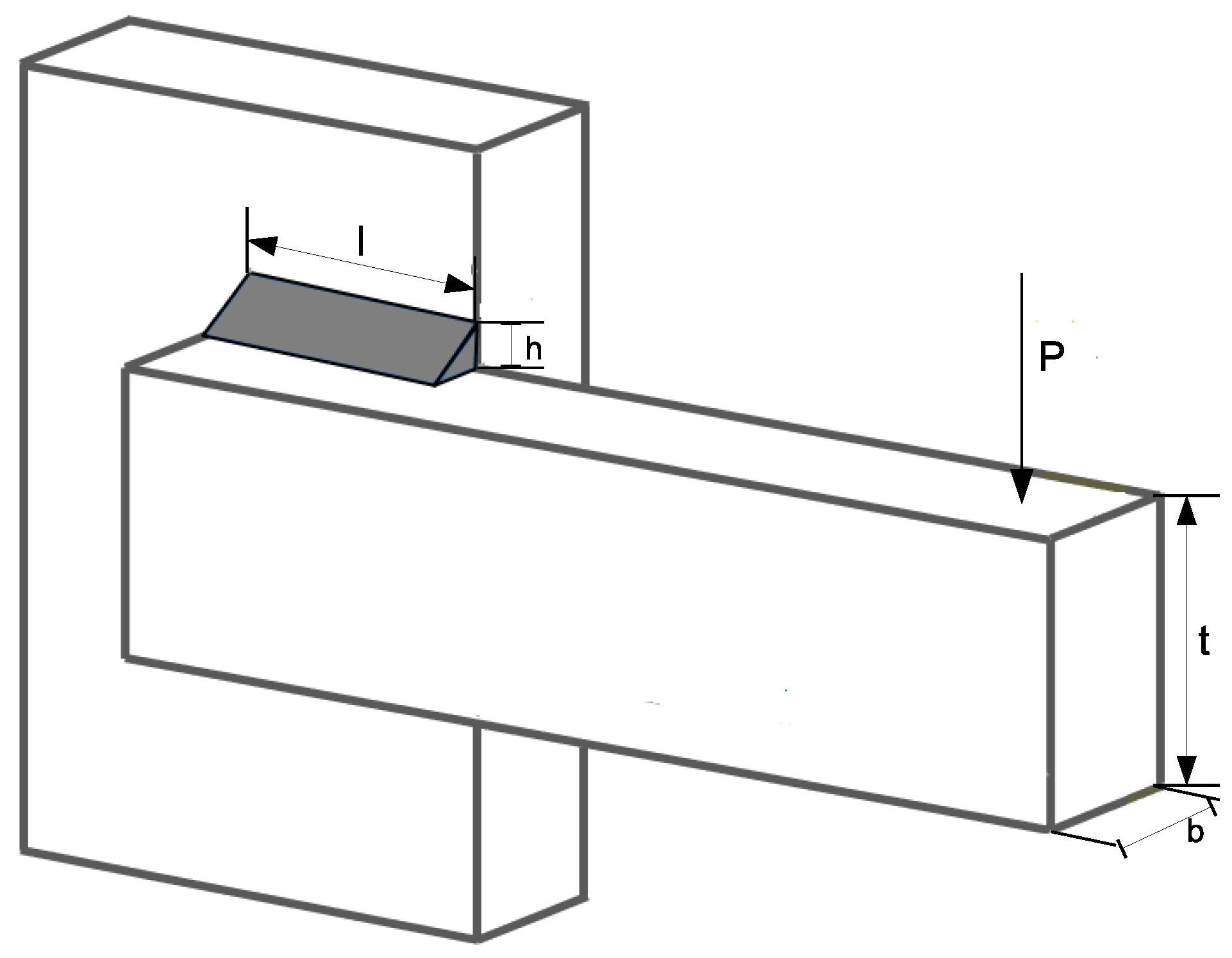
4.2.2. Welded Beam Design Problem

The welded beam design problem is depicted in Figure 9. The cost of manufacturing and assembling the welded beams must be minimized by considering the welding work, material, and labor cost. The variables to be computed are the thickness of the weld (h), the length of the welded joint (l), the width of the beam (t), and the thickness of the beam (b). The optimization problem is formulated as in (6), where $\tau \left(x\right)$ is the shear stress in the weld, ${\tau }_{max}$ is the allowable shear stress of the weld, $\sigma \left(x\right)$ is the normal stress in the beam, ${\sigma }_{max}$ is the allowable normal stress for the beam material, $P_c\left(x\right)$ is the bar buckling load, P is the load, $\delta \left(x\right)$ is the beam end deflection, and ${\delta }_{max}$ is the allowable beam end deflection. Some auxiliary functions and constant values used to solve the welded beam design problem are given in (7).

$$\begin{array}{cc}\hfill & \mathrm{Welded}\mathrm{beam}\mathrm{design}\mathrm{problem}:\hfill \\ \hfill F& =1.10471x_1^2{x}_2+0.04811x_3{x}_4(14.0+x_2)\hfill \\ \hfill & x_1=h,x_2=l,x_3=t,x_4=b\hfill \\ \hfill & \mathrm{Constraints}:\hfill \\ \hfill g_1& =\tau \left(x\right)-{\tau }_{max}\le 0\hfill \\ \hfill g_2& =\sigma \left(x\right)-{\sigma }_{max}\le 0\hfill \\ \hfill g_3& =x_1-x_4\le 0\hfill \\ \hfill g_4& =0.10471x_1^2+0.04811x_3{x}_4(14.0+x_2)-5.0\le 0\hfill \\ \hfill g_5& =0.125-x_1\le 0\hfill \\ \hfill g_6& =\delta \left(x\right)-{\delta }_{max}\le 0\hfill \\ \hfill g_7& =P\left(x\right)-P_c\left(x\right)\le 0\hfill \\ \hfill & 0.1\le x_1,x_4\le 2.0\hfill \\ \hfill & 0.1\le x_2,x_3\le 10.0\hfill \end{array}$$

(6)

$$\begin{array}{cc}\hfill & \mathrm{Functions}\mathrm{and}\mathrm{constants}\mathrm{of}\mathrm{welded}\mathrm{beam}\mathrm{problem}:\hfill \\ \hfill \tau \left(x\right)& =\sqrt{{\left({\tau }^{\prime }\right)}^2+2{\tau }^{\prime }{\tau }^{″}\frac{x_2}{2R}+{\left({\tau }^{″}\right)}^2};\hfill \\ \hfill {\tau }^{\prime }& =\frac{P}{\sqrt{2}{x}_1{x}_2};{\tau }^{″}=\frac{MR}{J}\hfill \\ \hfill M& =P\left(L+\frac{x_2}{2}\right);R=\sqrt{\frac{x_2^2}{4}+{\left(\frac{x_1+x_3}{2}\right)}^2}\hfill \\ \hfill J& =2\left\{\sqrt{2}{x}_1{x}_2\left[\frac{x_2^2}{12}+{\left(\frac{x_1+x_3}{2}\right)}^2\right]\right\}\hfill \\ \hfill \sigma \left(x\right)& =\frac{6PL}{x_4{x}_3^2}\hfill \\ \hfill \delta \left(x\right)& =\frac{4P{L}^3}{E{x}_3^3{x}_4}\hfill \\ \hfill P_c\left(x\right)& =\frac{4.013E\sqrt{\frac{x_3^2{x}_4^6}{36}}}{L^2}\left(1-\frac{x_3}{2L}\sqrt{\frac{E}{4G}}\right)\hfill \\ \hfill P& =6000lb;L=14in;{\delta }_{max}=0.25in\hfill \\ \hfill E& =30e^{+6}psi;G=12e^{+6}psi\hfill \\ \hfill {\tau }_{max}& =13,600psi;{\sigma }_{max}=30,000psi\hfill \end{array}$$

(7)

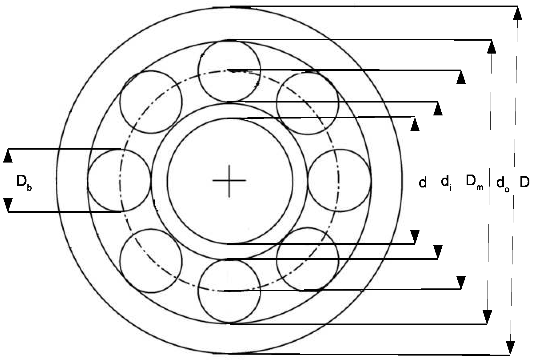
4.2.3. Rolling Element Bearing Design Problem

The rolling element bearing design problem is a maximization problem aimed to maximize the dynamic load capacity of a rolling element bearing. This problem, depicted in Figure 10, has five decision variables, namely pitch diameter ($D_m$), ball diameter ($D_b$), number of balls (Z), curvature radius coefficient of inner raceway groove ($f_i=r_i/D_b$), curvature radius coefficient of outer raceway groove ($f_o=r_o/D_b$), and the inner and outer ring groove curvature ratio $r_i$ and $r_o$, respectively. In addition, it has five constraints constants, $K_{Dmin}$, $K_{Dmax}$, $ϵ$, e and $\psi$. This problem can be formulated as in (8).

$$\begin{array}{cc}\hfill & \mathrm{Rolling}\mathrm{element}\mathrm{bearing}\mathrm{design}\mathrm{problem}:\hfill \\ \hfill f& =f_c{x}_3^{2/3}{x}_2^{1.8};\mathrm{if}{x}_2\le 25.4\hfill \\ \hfill f& =3.647f_c{x}_3^{2/3}{x}_2^{1.4};\mathrm{if}{x}_2>25.4\hfill \\ \hfill & x_1=D_m,x_2=D_b,x_3=Z,x_4=f_i,x_5=f_o\hfill \\ \hfill & \mathrm{Constraints}:\hfill \\ \hfill g_1& =\frac{{\varphi }_0}{2{sin}^{-1}\frac{x_2}{x_1}}-x_3+1\ge 0\hfill \\ \hfill g_2& =2.0x_2-x_6(D-d)\ge 0\hfill \\ \hfill g_3& =x_7(D-d)-2.0x_2\ge 0\hfill \\ \hfill g_4& =x_{10}{B}_w-x_2\ge 0\hfill \\ \hfill g_5& =x_1-0.5(D+d)\ge 0\hfill \\ \hfill g_6& =(0.5+x_9)(D+d)-x_1\ge 0\hfill \\ \hfill g_7& =0.5(D-x_1-x_2)-x_8{x}_2\ge 0\hfill \\ \hfill g_8& =x_4-0.515\ge 0\hfill \\ \hfill g_9& =x_5-0.515\ge 0\hfill \\ \hfill & x_6=K_{Dmin},x_7=K_{Dmax},x_8=ϵ,x_9=e,x_5=\psi \hfill \end{array}$$

(8)

$$\begin{array}{cc}\hfill & \mathrm{Auxiliary}\mathrm{functions}\mathrm{and}\mathrm{constant}\mathrm{values}\mathrm{of}\mathrm{rolling}\mathrm{problem}:\hfill \\ \hfill \gamma & =\frac{D_{b}cos\alpha }{D_m}\hfill \\ \hfill f_c=& 37.91\times {\left\{1+{\left[1.04{\left(\frac{1-\gamma }{1+\gamma }\right)}^{1.72}{\left(\frac{f_i(2f_o-1)}{f_o(2f_i-1)}\right)}^{0.41}\right]}^{10/3}\right\}}^{-0.3}\times \left\{\left(\frac{{\gamma }^{0.3}{(1-\gamma )}^{1.39}}{{(1+\gamma )}^{1/3}}\right){\left(\frac{2f_i}{2f_i-1}\right)}^{0.41}\right\}\hfill \\ \hfill T& =D-d-\left(2.0x_2\right)\hfill \\ \hfill {\varphi }_0& =2\pi -2{cos}^{-1}\left(\frac{{\left(\frac{D-d}{2}-\frac{3T}{4}\right)}^2+{\left(\frac{D}{2}-\frac{T}{4}-x_2\right)}^2-{\left(\frac{d}{2}+\frac{T}{4}\right)}^2}{2\left(\frac{D-d}{3}-\frac{3T}{4}\right)\left(\frac{D}{2}-\frac{T}{4}-x_2\right)}\right)\hfill \\ \hfill D& =160;d=90;B_w=30;\alpha =0\hfill \\ \hfill & 90.0\le x_1\le 150.0\hfill \\ \hfill & 10.5\le x_2\le 31.5\hfill \\ \hfill & 4\le x_3\le 50\hfill \\ \hfill & 0.515\le x_4,x_5\le 0.6\hfill \\ \hfill & 0.4\le x_6\le 0.5\hfill \\ \hfill & 0.6\le x_7\le 0.7\hfill \\ \hfill & 0.3\le x_8\le 0.4\hfill \\ \hfill & 0.02\le x_9\le 1.0\hfill \\ \hfill & 0.6\le x_{10}\le 0.85\hfill \end{array}$$

(9)

5. Numerical Experiments

All the numerical experiments have been obtained in Fujitsu Server PRIMERGY TX300 S8 Tower Server. This platform is a multicore platform equipped with a D2949-B1 motherboard with two CPU sockets. In each CPU the processor installed is an Intel(R) Xeon(R) CPU E5-2620 v2 @ 2.10 GHz, with 15 MB Intel Smart Cache. Each processor is composed of 6 physical cores, resulting in a total number of 12 physical cores in the system. The Intel Hyper-Threading Technology is enabled, the number of threads per physical core is 2, therefore the maximum number of processes (or threads) should not exceed 24, in order to obtain the best possible computational performance. The main memory size is 32 GB of DDR3. All the developments, both sequential and parallel, were implemented in the C programming language, using the GCC v.4.4.7 [45]. The OpenMP API v3.1 [46] has been used to develop parallel algorithms. Therefore, all the data in tables and figures included in this section have been obtained running simulations in this platform. In addition, for the computational results to be reliable, the Sun Grid Engine queuing system has been used.

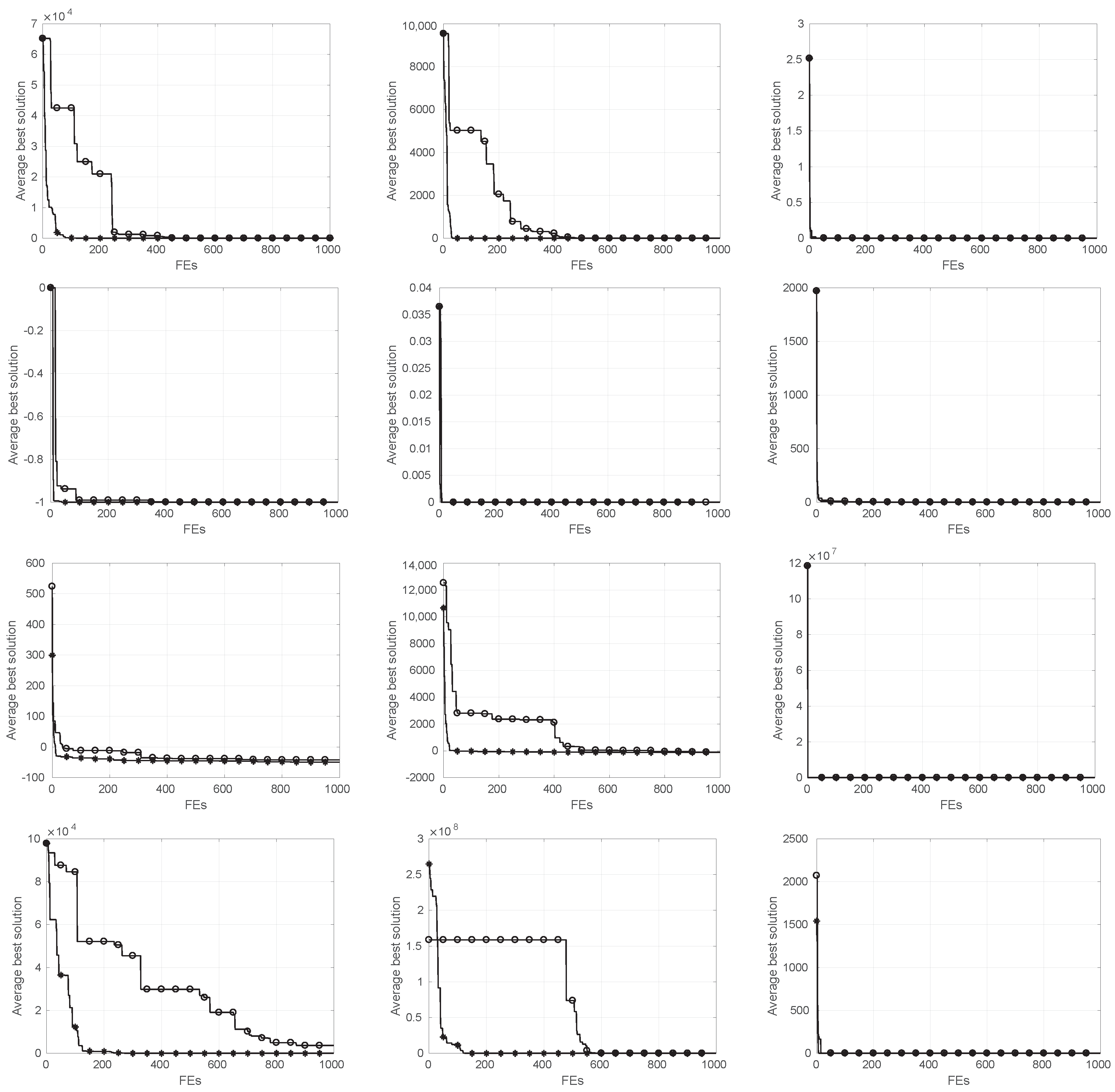
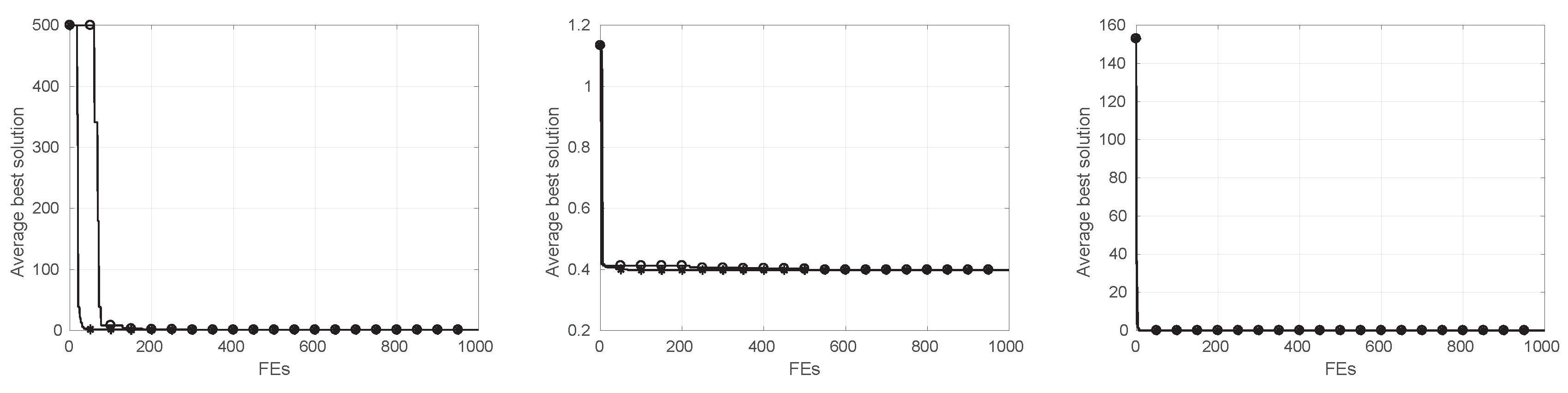
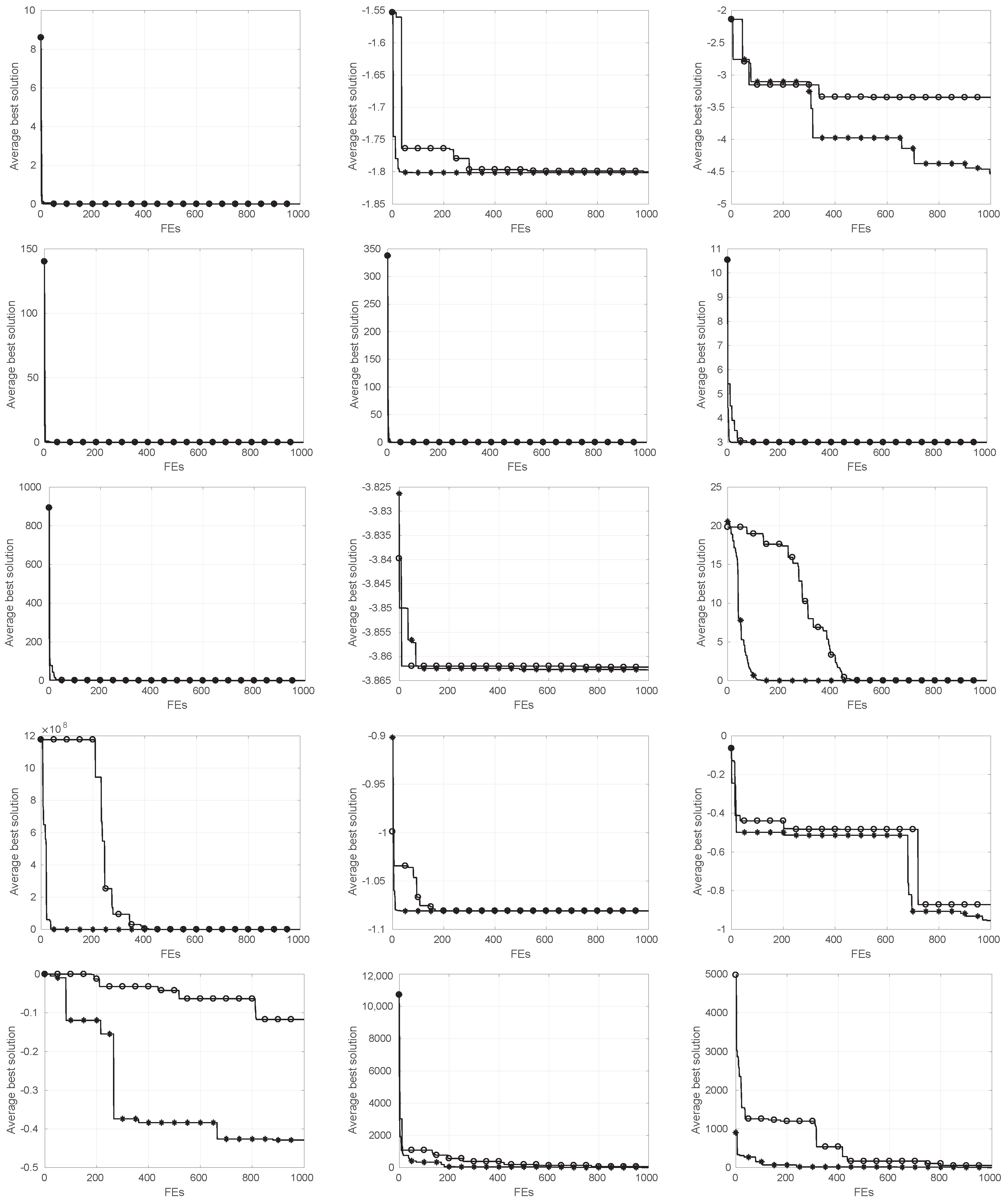
5.1. Comparative Analysis ESCA vs. SCA

First, the computational costs of the SCA algorithm and the proposed ESCA algorithm are examined in

Table 3. Computational times (s.) for sequential SCA and ESCA algorithms.

	Population Size
	60		120		240
	SCA	ESCA	SCA	ESCA	SCA	ESCA
$f_1$	349.3	308.8	683.5	711.5	1432.5	1325.7
$f_2$	388.5	312.9	739.0	668.4	1474.9	1405.0
$f_3$	25.2	23.4	50.4	46.8	100.6	93.6
$f_4$	27.8	26.4	55.6	52.8	111.2	105.6
$f_5$	33.9	31.4	68.8	70.2	131.7	138.5
$f_6$	31.3	28.6	62.4	57.1	124.7	114.1
$f_7$	48.6	44.1	96.9	87.9	193.7	179.3
$f_8$	80.5	69.8	160.0	140.8	321.4	279.2
$f_9$	144.7	132.7	280.6	268.0	558.3	530.3
$f_{10}$	374.5	413.7	773.6	815.8	1562.5	1657.5
$f_{11}$	223.1	208.3	442.6	416.4	884.5	833.1
$f_{12}$	38.4	36.4	77.9	72.5	154.9	145.5
$f_{13}$	461.7	466.7	923.8	933.9	1845.8	1867.0
$f_{14}$	19.7	18.9	39.5	37.8	79.1	75.6
$f_{15}$	17.8	17.1	33.9	33.9	70.7	68.0
$f_{16}$	15.5	14.6	31.2	29.1	62.0	58.1
$f_{17}$	72.3	55.6	144.7	111.0	291.4	221.9
$f_{18}$	174.7	125.1	309.0	280.3	620.4	493.1
$f_{19}$	18.7	16.5	36.1	32.2	72.2	70.2
$f_{20}$	17.6	16.8	35.2	31.2	69.9	59.7
$f_{21}$	16.3	15.3	32.6	30.6	65.1	61.0
$f_{22}$	105.5	101.8	212.0	205.5	419.7	409.7
$f_{23}$	36.3	36.5	72.0	73.2	146.1	146.3
$f_{24}$	125.6	123.2	251.6	246.3	501.5	493.8
$f_{25}$	406.4	321.7	812.3	674.4	1707.8	1321.8
$f_{26}$	56.4	57.1	113.3	113.5	225.6	227.2
$f_{27}$	82.0	82.0	164.3	164.1	331.8	328.8
$f_{28}$	130.6	118.5	262.2	236.1	523.4	473.2
$f_{29}$	174.0	168.7	346.9	339.4	700.0	675.1
$f_{30}$	583.4	568.9	1165.5	1134.6	2334.1	2290.9

. This table shows the computing time cost when optimizing the benchmark test reported in Section 4 with population sizes of 240, 120, and 60. The number of generations was 50,000, and the number of independent runs was 30. The results in Table 3 point that the proposed ESCA algorithm does not increase the computing cost compared to the SCA algorithm. On the contrary, in more than 80% of the experiments conducted, the computational cost decreases.

Once it has been proven that the proposed method decreases the computational cost of the SCA algorithm, the optimization behavior is investigated by comparing both methods in

Table 4. Number of function evaluations for an error < 1 $\times {10}^{-3}$ (* < 1 $\times {10}^2$).

	Population Size
	240		120		60
	SCA	ESCA	SCA	ESCA	SCA	ESCA
$f_1$	3,639,144	75,384	1,842,864	48,504	971,802	28,074
$f_2$	3,596,880	73,464	1,808,004	43,500	988,380	24,888
$f_3$	24,000	2136	24,888	3072	13,878	2082
$f_4$	306,912	4152	218,220	3432	239,166	2088
$f_5$	1584	840	756	564	540	312
$f_6$	–	9,627,227	–	4,450,577	–	2,654,280
$f_7$ *	3888	960	5724	612	3222	354
$f_8$ *	5,031,792	317,376	2,684,760	190,053	1,565,184	196,337
$f_9$	1,528,656	16,848	848,544	9708	490,854	6420
$f_{10}$	5,048,616	739,296	2,623,800	462,456	1,400,712	311,640
$f_{11}$ *	3,677,160	78,720	1,906,380	45,828	–	32,424
$f_{12}$	–	6,186,240	–	4,982,240	–	2,624,640
$f_{13}$	571,008	14,088	547,320	6288	236,148	36,126
$f_{14}$	70,392	1920	118,296	2256	52,782	1998
$f_{15}$	5928	2352	2964	1380	2262	762
$f_{16}$	187,560	3120	236,952	2508	131,712	2400
$f_{17}$	401,688	3888	419,220	1812	236,400	2910
$f_{18}$ *	480	480	240	240	120	120
$f_{19}$	6120	2448	3624	1392	1896	882
$f_{20}$	5160	2112	4560	1296	2340	834
$f_{21}$	26,856	2040	28,596	1080	15,924	912
$f_{22}$	–	3,966,264	–	3,528,912	–	1,907,900
$f_{23}$	7920	57,090	3,739,200	81,345	123,720	27,760
$f_{24}$	2,290,464	30,408	1,207,956	17,940	668,790	8304
$f_{25}$ *	3,591,960	46,032	1,952,616	33,756	951,708	17,022
$f_{26}$	20,400	9672	21,744	4848	10,193	2208
$f_{27}$	–	6,840,528	–	5,366,040	–	2,930,112
$f_{28}$	480	480	252	252	120	120
$f_{29}$ *	1,127,832	24,168	1,148,604	27,672	840,288	26,940
$f_{30}$ *	–	9,787,467	–	5,338,960	–	2,939,910

. This table shows the number of function evaluations for an error of less than <1 $\times {10}^{-3}$(for functions marked with * an error less than <1 $\times {10}^2$), with population sizes of 240, 120, and 60. Fewer function evaluations are required when the ESCA method is used instead of the SCA method. The dramatic decrease, particularly for the functions that require more evaluations, is higher than 100×, demonstrating the significant improvement of the SCA’s optimization behavior.

To perform a parallel efficiency analysis of both parallel proposals, experimental tests are conducted using the same parameters as those used so far, i.e., population sizes of 240, 120, and 60. The number of generations is equal to 50,000, and the number of independent runs is 30. The parallel speed-up values for the data sharing parallel algorithm, depending on the total population size ($popInitSize$) and the number of processes ($NoCs$), are exhibited in

Table 5. Parallel speed-up for parallel data sharing algorithm.

	Population Size
	240			120			60
	$\mathit{NoCs}$
	2	6	12	2	6	12	2	6	12
$f_1$	2.0	5.7	10.4	2.0	5.7	11.4	1.8	5.0	9.7
$f_2$	2.0	5.8	10.9	1.8	5.5	10.5	2.0	4.9	9.3
$f_3$	1.9	4.9	6.9	1.9	4.6	4.5	1.9	3.7	2.5
$f_4$	2.0	5.5	10.9	1.9	5.5	10.3	1.6	5.3	3.8
$f_5$	1.9	5.0	9.0	1.8	4.9	7.4	1.6	4.2	3.7
$f_6$	2.0	5.5	10.9	1.9	5.4	10.4	1.9	5.4	3.6
$f_7$	1.3	3.3	4.5	1.9	4.7	5.1	1.9	4.1	3.4
$f_8$	2.0	5.4	9.9	2.0	5.3	9.0	1.9	5.1	6.8
$f_9$	1.9	5.2	10.2	1.8	5.3	10.1	1.9	5.1	9.2
$f_{10}$	2.0	5.5	11.0	1.9	5.4	10.6	2.0	5.5	10.4
$f_{11}$	2.0	5.5	11.0	2.0	5.5	10.9	2.0	5.5	10.9
$f_{12}$	2.0	5.3	9.1	1.9	5.1	7.2	1.9	4.6	4.0
$f_{13}$	2.0	5.5	11.1	2.0	5.5	11.0	2.0	5.5	10.8
$f_{14}$	2.0	5.5	10.7	2.0	5.4	8.8	1.9	5.2	2.4
$f_{15}$	1.9	5.4	10.2	2.0	5.7	6.3	2.0	5.2	2.2
$f_{16}$	1.9	5.5	10.4	1.9	5.3	5.2	1.9	5.1	1.8
$f_{17}$	2.0	5.4	9.5	2.0	5.2	8.2	1.9	4.8	5.8
$f_{18}$	1.9	5.4	9.3	1.9	6.0	8.7	1.7	4.8	6.0
$f_{19}$	2.0	5.1	7.1	1.7	4.3	3.8	1.5	3.7	1.9
$f_{20}$	1.7	4.8	6.4	1.8	4.5	3.8	1.6	4.1	1.9
$f_{21}$	1.9	5.1	6.4	1.9	4.6	3.5	1.9	3.6	1.7
$f_{22}$	1.9	5.2	10.2	1.9	5.3	9.9	1.9	5.1	8.8
$f_{23}$	2.0	5.5	10.6	2.0	5.4	10.2	1.9	5.4	8.9
$f_{24}$	2.0	5.5	10.4	1.9	5.4	9.6	2.0	5.2	8.5
$f_{25}$	2.0	5.6	10.4	2.0	5.5	10.0	2.0	5.2	9.1
$f_{26}$	2.0	5.2	8.4	1.9	5.0	7.2	1.9	4.8	5.6
$f_{27}$	2.0	5.4	9.8	2.0	5.1	8.7	2.0	5.0	6.9
$f_{28}$	2.0	5.5	10.9	1.9	5.5	10.9	1.9	5.4	10.8
$f_{29}$	2.0	5.5	11.0	2.0	5.5	10.6	2.0	5.4	10.4
$f_{30}$	2.0	5.6	11.1	2.0	5.5	11.0	2.0	5.5	10.9

. The obtained speed-up values are close to ideal ones for the largest population size. These values slightly decrease, in most cases, as the population size decreases. However, the values significantly degrade when 12 parallel processes are used for the smaller population size and lower computing cost functions.

The parallel asynchronous algorithm’s speed-up values, shown in

Table 6. Parallel speed-up for asynchronous parallel algorithm.

	Population Size
	240			120			60
	$\mathit{NoCs}$
	2	6	12	2	6	12	2	6	12
$f_1$	2.0	5.7	11.6	2.0	5.8	11.6	1.9	5.7	11.2
$f_2$	1.9	5.5	11.4	1.9	5.6	11.2	1.9	5.2	10.5
$f_3$	1.9	5.5	11.0	1.9	5.5	11.0	1.9	5.5	8.2
$f_4$	1.9	5.5	11.0	2.0	5.5	11.0	2.0	5.5	11.0
$f_5$	1.9	5.5	11.0	2.0	5.5	11.1	1.8	5.5	11.0
$f_6$	1.9	5.5	11.0	2.0	5.5	11.1	2.0	5.5	11.0
$f_7$	1.3	3.6	7.3	2.0	5.5	11.0	1.9	5.5	11.0
$f_8$	1.9	5.5	11.0	2.0	5.5	11.1	2.0	5.5	11.1
$f_9$	1.9	5.6	11.1	2.1	5.3	10.6	1.9	5.2	10.7
$f_{10}$	1.9	5.4	10.9	2.0	5.6	11.1	2.0	5.5	10.9
$f_{11}$	1.9	5.5	10.9	2.0	5.5	11.1	1.9	5.5	11.1
$f_{12}$	1.9	5.5	10.7	2.0	5.5	11.0	2.0	5.5	10.9
$f_{13}$	1.9	5.5	11.0	2.0	5.5	11.0	2.0	5.5	11.1
$f_{14}$	1.9	5.5	10.9	2.0	5.5	11.0	1.9	5.5	10.9
$f_{15}$	1.9	5.4	10.9	1.8	5.2	10.3	1.8	5.4	10.9
$f_{16}$	1.9	5.5	11.0	1.9	5.5	10.9	1.9	5.5	10.8
$f_{17}$	1.9	5.5	11.1	2.0	5.5	10.7	2.0	5.5	10.9
$f_{18}$	1.9	5.6	11.3	2.0	5.6	11.1	2.0	5.6	11.3
$f_{19}$	1.8	5.1	9.9	1.9	5.4	10.5	1.9	5.0	9.9
$f_{20}$	1.9	5.3	10.4	2.0	5.5	11.0	1.9	5.5	10.9
$f_{21}$	1.9	5.5	11.0	2.0	5.5	10.2	1.9	5.5	10.9
$f_{22}$	1.9	5.2	10.4	1.9	5.2	10.5	1.9	5.3	10.3
$f_{23}$	1.9	5.4	10.7	2.0	5.5	10.9	2.0	5.5	10.8
$f_{24}$	1.9	5.5	11.0	2.0	5.6	11.2	2.0	5.5	11.0
$f_{25}$	1.9	5.4	10.9	2.0	5.5	11.1	1.9	5.6	11.0
$f_{26}$	1.9	5.5	11.0	2.0	5.5	11.0	1.9	5.5	11.0
$f_{27}$	1.9	5.5	10.9	2.0	5.4	11.0	2.0	5.5	11.0
$f_{28}$	1.9	5.5	11.0	2.0	5.5	11.1	1.9	5.6	11.1
$f_{29}$	1.9	5.5	11.0	2.0	5.5	11.0	2.0	5.5	11.0
$f_{30}$	1.9	5.5	10.9	2.0	5.6	11.0	2.0	5.6	11.1

, remain close to the ideal values when the number of concurrent processes is increased or when the population size is decreased. Note that this behavior implies outstanding parallel scalability.

Considering the outstanding parallel performance results obtained for the parallel asynchronous algorithm using the 12 available physical cores (see Table 6), it can be concluded that the parallel scalability of the asynchronous algorithm allows increasing the number of processes efficiently. However, the results shown in Table 4 confirm that the size of the subpopulations requires a minimum dimension, which depends on the optimization algorithm and the problem under consideration. Algorithm 6 has been proposed to increase the number of processes without reducing the size of the subpopulations. To implement the inner level of parallelism of Algorithm 6, nested parallelism can be applied using OpenMP features. This strategy has been discarded due to poor experimental results that excessively degrade parallel scalability. When using nested parallelism the generation of each nested parallel region involves computational overhead [47]. The poor experimental results are due to many nested regions ($numGenerations\times NoCs$) and the insufficient computational cost of each nested parallel region. Note that this computational cost depends on the considered algorithm (quasi-non-variable cost) and the objective function.

The two-level parallel algorithm generates a parallel region of $NoCs\times inCs$ processes, organized into $NoCs$ groups of $inCs$ processes each. In each group, only one process works outside the inner parallel region, while all the processes in the group cooperate in the processing associated with the inner level of parallelism (lines 13–29 of Algorithm 6).

As mentioned above, the used parallel platform has two processors with six physical cores each. Hyperthreading can be enabled, allowing to run two processes (or threads) per core efficiently. Thus, it can be run up to 24 concurrent processes without excessively degrading the computer platform’s efficiency. Using hyperthreading and fine-grained parallelism, such as the proposed two-level algorithm, the strategy of thread placement on the cores may be relevant. To control the strategy of process placement in the cores, OpenMP affinity features are used. Figure 11a shows that the platform’s architecture is equipped with two processors of six physical cores and twelve logical cores each. An example of thread placement of 5 processes when no affinity is used is shown in Figure 11b, in which the operating system decides the process placement. There is no problem in this thread placement if neither hyperthreading nor fine-grained parallelism are used.

For instance, using 20 processes organized into 5 groups of 4 processes, a thread placement option without using affinity features is displayed in Figure 12a. To optimize parallel performance, the optimal thread placement can be forced using OpenMP affinity features as shown in Figure 12b.

Table 7. Parallel speed-up for the two-level parallel algorithm using groups of processes. Population size = 240.

	16 Processes			20 Processes
$\mathit{NoCs};\mathit{inCs}$	8;2	4;4	2;8	10;2	5;4	4;5	2;10
$f_1$	12.5	12.5	12.1	15.9	15.0	15.2	15.2
$f_2$	12.5	12.1	11.6	14.4	14.8	15.0	14.7
$f_{10}$	11.9	11.8	11.8	14.7	14.7	14.7	14.7
$f_{13}$	10.1	10.0	9.7	12.7	12.4	12.3	11.7
$f_{30}$	12.2	12.1	12.2	15.3	15.2	15.1	15.1

shows the parallel speed-up when more than 12 processes are used, i.e., using hyperthreading for the highest computational cost functions. Results manifested in Table 7 have been obtained using 16 and 20 processes by varying the number of groups ($NoCs$) and consequently varying the number of processes per group ($inCs$). Important conclusions can be drawn by analyzing the results of this table: remarkable scalability is obtained through the two-level parallel algorithm, even using logical cores (hyperthreading); although the parallel performance allows setting the $NoCs$ value (i.e., number of groups) according to the desired size of the subpopulations, i.e., according to the optimization performance rather than parallel behavior. All efficiency values are above 72%, except for the Foxholes function ($f_{13}$), characterized by having only two design variables (see Table 1), which penalizes fine-grained parallelism. Although both fine-grained parallelism and hyperthreading slightly penalize parallel efficiency, a remarkable average greater than 75% parallel efficiency is obtained. The average efficiency barely decreases as the number of processes increases from 16 to 20, resulting in a slight fall of the average efficiency from 75.6% to 74.9%, i.e., the outstanding parallel scalability is maintained.

This outstanding behavior is confirmed by the results shown in

Table 8. Parallel speed-up for the two-level parallel algorithm using groups of processes. Population size = 240. Number of processes = 24.

	24 Processes
$\mathit{NoCs};\mathit{inCs}$	12;2	6;4	4;6	2;12
$f_1$	19.0	18.3	18.7	17.4
$f_2$	18.0	17.4	16.9	18.0
$f_{10}$	17.6	17.6	17.4	17.4
$f_{30}$	18.2	18.0	18.1	17.8

, which are the results conducted on all the available threads (24) when hyperthreading is activated. It is found that the two-level parallel algorithm has remarkable parallel scalability with an average parallel efficiency of 74.4%.

Table 9. Sharing data parallel algorithm: number of function evaluations for error <1 $\times {10}^{-3}$ (* < 1 $\times {10}^2$). $popInitSize=240$.

	$\mathit{NoCs}$
	1	2	6	12
$f_1$	75,384	80,657	83,776	76,385
$f_2$	73,464	70,135	73,034	60,717
$f_3$	2136	2120	2128	2200
$f_4$	4152	4889	4005	3507
$f_5$	840	842	687	312
$f_6$	9,627,227	9,966,401	9,430,103	9,876,351
$f_7$ *	960	762	722	583
$f_8$ *	317,376	374,307	255,284	324,357
$f_9$	16,848	16,516	17,853	17,829
$f_{10}$	739,296	854,471	780,928	743,569
$f_{11}$ *	78,720	65,643	75,129	76,902
$f_{12}$	6,186,240	7,359,497	8,535,793	5,457,901
$f_{13}$	14,088	9603	7294	11,392
$f_{14}$	1920	2042	3831	2259
$f_{15}$	2352	2144	2453	1722
$f_{16}$	3120	3342	3328	4471
$f_{17}$	3888	3517	3275	2470
$f_{18}$ *	480	456	453	373
$f_{19}$	2448	2259	2192	1990
$f_{20}$	2112	2262	2031	1892
$f_{21}$	2040	1732	1601	974
$f_{22}$	3,966,264	3,298,233	5,086,208	7,588,192
$f_{23}$	57,090	3134	4069	3396
$f_{24}$	30,408	28,982	30,281	30,248
$f_{25}$ *	46,032	56,975	35,157	41,468
$f_{26}$	9672	15,605	13,573	10,713
$f_{27}$	6,840,528	10,618,500	3,333,940	8,731,516
$f_{28}$	480	440	462	164
$f_{29}$ *	24,168	30,604	25,408	26,676
$f_{30}$ *	9,787,467	8,810,661	8,232,263	10,546,564

and

Table 10. Sharing data parallel algorithm: number of function evaluations for error <1 $\times {10}^{-3}$ (* < 1 $\times {10}^2$). popInitSize = 60.

	$\mathit{NoCs}$
	1	2	6	12
$f_1$	28,074	32,624	28,419	28,128
$f_2$	24,888	24,323	25,030	22,209
$f_3$	2082	2361	1867	1670
$f_4$	2088	2319	1762	2220
$f_5$	312	314	250	173
$f_6$	2,654,280	1,896,252	2,914,210	1,951,487
$f_7$ *	354	325	430	262
$f_8$ *	196,337	279,480	347,191	238,579
$f_9$	6420	7143	6844	7113
$f_{10}$	311,640	262,261	308,376	310,209
$f_{11}$ *	32,424	28,081	28,738	32,903
$f_{12}$	2,624,640	2,353,703	2,680,174	2,202,838
$f_{13}$	36,126	18,554	6345	34,818
$f_{14}$	1998	1944	1917	2689
$f_{15}$	762	820	753	520
$f_{16}$	2400	2503	3393	2781
$f_{17}$	2910	1271	2745	2865
$f_{18}$ *	120	114	105	63
$f_{19}$	882	762	879	604
$f_{20}$	834	807	812	629
$f_{21}$	912	691	743	543
$f_{22}$	1,907,900	1,110,490	1,874,520	2,209,849
$f_{23}$	27,760	3956	2633	3782
$f_{24}$	8304	9840	10,120	9041
$f_{25}$ *	17,022	21,353	28,550	17,609
$f_{26}$	2208	2626	9685	1920
$f_{27}$	2,930,112	2,842,249	2,925,193	2,806,709
$f_{28}$	120	113	113	37
$f_{29}$ *	26,940	12,415	17,103	17,228
$f_{30}$ *	2,939,910	2,650,149	2,863,317	2,815,149

show the number of functions evaluations required by the data sharing parallel algorithm to obtain an error of less than $1\times {10}^{-3}$ ($1\times {10}^2$ for functions marked with an asterisk), when the total population size is 240 ($popInitSize=240$) and 60 ($popInitSize=60$), respectively. These results show that the number of concurrent processes does not modify the optimization behavior. The heuristic nature of the proposed optimization algorithm results in different evaluations for the same function depending on the concurrent processes.

Table 11. Asynchronous parallel algorithm: number of function evaluations for error <1 $\times {10}^{-3}$ (* < 1 $\times {10}^2$). $popInitSize=240$.

	$\mathit{NoCs}$
	1	2	6	12
$f_1$	80,136	83,277	90,626	84,218
$f_2$	73,824	72,792	73,927	74,209
$f_3$	2568	2578	2989	3313
$f_4$	3264	5795	5436	5963
$f_5$	816	633	750	410
$f_6$	8,974,650	10,097,595	10,025,662	11,314,284
$f_7$ *	1032	759	897	481
$f_8$ *	253,920	34,7465	61,2221	86,7391
$f_9$	17,184	16,644	23,193	25,164
$f_{10}$	71,4336	85,8736	1,078,127	1,252,559
$f_{11}$ *	64,656	77,582	88,175	10,3109
$f_{12}$	8,937,680	7,699,045	10,565,357	11,289,390
$f_{13}$	46,872	10,347	17,452	20,750
$f_{14}$	1992	3554	4702	5277
$f_{15}$	2256	2277	2656	1922
$f_{16}$	4896	4869	6881	6861
$f_{17}$	3264	3640	4408	5952
$f_{18}$ *	480	411	413	306
$f_{19}$	2256	2204	2452	2353
$f_{20}$	2304	2441	2661	1826
$f_{21}$	1896	1590	2347	2041
$f_{22}$	4,256,610	7,094,932	7,742,422	6,726,769
$f_{23}$	10,1640	49,884	14,750	30,406
$f_{24}$	31,152	32,214	32,039	33,949
$f_{25}$ *	37,752	47,883	46,427	41,350
$f_{26}$	8592	3266	2386	3399
$f_{27}$	8,689,680	9,215,379	10,203,567	10,787,817
$f_{28}$	528	456	444	199
$f_{29}$ *	21,624	29,572	58,600	46,029
$f_{30}$ *	10,729,470	10,103,632	10,519,594	9,802,382

and

Table 12. Asynchronous parallel algorithm: number of function evaluations for error <1 $\times {10}^{-3}$ (* < 1 $\times {10}^2$). $popInitSize=60$.

	$\mathit{NoCs}$
	1	2	6	12
$f_1$	28,308	25,754	37,605	33,407
$f_2$	24,684	25,346	26,985	26,891
$f_3$	1644	1163	1876	3188
$f_4$	2778	2239	4294	4816
$f_5$	378	307	228	308
$f_6$	2,742,830	2,918,138	2,936,681
$f_7$ *	402	415	376	156
$f_8$ *	216,387	314,711	495,643	602,778
$f_9$	6822	6827	9873	11,370
$f_{10}$	314,562	316,765	415,446	413,730
$f_{11}$ *	28,338	26,143	29,280	35,931
$f_{12}$	2,444,835	2,056,447	2,802,878	2,993,886
$f_{13}$	52,848	35,565	30,404	63,877
$f_{14}$	1680	2625	7972	5786
$f_{15}$	732	926	851	583
$f_{16}$	2736	6429	4814	8359
$f_{17}$	2790	3023	5588	9495
$f_{18}$ *	120	101	105	46
$f_{19}$	630	846	877	563
$f_{20}$	792	736	878	732
$f_{21}$	858	914	930	1437
$f_{22}$	1,089,000	1,850,238	2,757,559
$f_{23}$	1980	11,291	20,030	21,210
$f_{24}$	8940	9557	8676	11,540
$f_{25}$ *	17,652	21,631	17,447	17,945
$f_{26}$	3342	1151	2377	3869
$f_{27}$	2,918,580	2,865,679	2,970,869	2,779,579
$f_{28}$	120	116	105	30
$f_{29}$ *	23,586	22,921	42,961	59,068
$f_{30}$ *	2,782,130	2,885,935	2,631,535	2,801,275

listed the number of functions evaluations required by the asynchronous parallel algorithm for population sizes 240 ($popInitSize=240$) and 60 ($popInitSize=60$), respectively. It is clear that, unlike the sharing data-parallel algorithm, the ratio of convergence depends on the number of concurrent processes used for the asynchronous parallel algorithm. In addition, the convergence ratio slightly worsens as the number of concurrent processes increases, but the outstanding parallel scalability offsets this behavior. Note that this behavior depends on the subpopulation sizes, which depend on the population size.

As earlier recorded, the parallel asynchronous algorithm allows each thread to have its population size without sacrificing parallel performance and thus exploring populations of different characteristics, which could improve the optimization’s performance.

Table 13. Asynchronous parallel algorithm: number of function evaluations for error <1 $\times {10}^{-3}$, 6 processes and homogeneous and heterogeneous subpopulation sizes. $popInitSize=240$.

	Thread Id.
	0	1	2	3	4	5
	Subpopulation Sizes						# FEs
$f_6$	40	40	40	40	40	40	10,025,662
	80	60	40	30	20	10	8,365,248
$f_{22}$	40	40	40	40	40	40	7,742,422
	80	60	40	30	20	10	6,341,866
$f_{27}$	40	40	40	40	40	40	10,203,567
	80	60	40	30	20	10	9,941,450

compares the number of function evaluations (# FEs) for functions $f_6$, $f_{22}$, and $f_{27}$ when using homogeneous and heterogeneous subpopulation sizes. The latter improving the optimization performance. Moreover, not reaching a good solution due to small populations can be avoided by increasing the number of processes. For instance, 12 processes are used for $f_6$ and $f_{27}$ (see Table 12).

It is settled that the proposed parallel algorithms achieve a remarkable parallel performance without disordering the optimization behavior. Figure 13 and Figure 14 point the significant improvement in the convergence speed of the proposed ESCA algorithm compared to the SCA algorithm.

The last analysis discusses the optimization’s behavior when solving the engineering design problems described in Section 4.2.

Table 14. Convergence ratio for ESCA and SCA algorithms with different population sizes.

	Population Size
	60	120	240
	Pressure Vessel Problem
ESCA-10000	6060.2070	6060.7420	6059.9340
SCA-10000	6079.0610	6091.4340	6068.5540
ESCA-20000	6060.0950	6059.8290	6059.8000
SCA-20000	6065.7460	6066.9530	6069.2260
	Welded beam problem
ESCA-10000	1.728844	1.726625	1.726300
SCA-10000	1.748143	1.749394	1.747236
ESCA-20000	1.726585	1.726704	1.725514
SCA-20000	1.751480	1.747207	1.738482
	Rolling element bearing problem
ESCA-10000	81,706.17	81,798.38	81,832.05
SCA-10000	80,673.58	81,333.65	80,318.50
ESCA-20000	81,803.87	81,774.60	81,836.77
SCA-20000	80,224.49	80,335.60	81,086.44

compares the convergence ratio of the SCA and ESCA methods when only 10,000 and 20,000 generations are processed. As can be observed from this table, the ESCA outperforms the SCA algorithm in terms of convergence ratio. Similar results are obtained when optimizing the 30 benchmark functions. This behavior confirms that our proposal significantly boosts the SCA algorithm.

As for solution accuracy, the results on benchmark functions and challenging engineering problems are listed in

Table 15. Average values for unconstrained and constrained problems obtained by ESCA and SCA.

	Population Size
	60		120		240
	SCA	ESCA	SCA	ESCA	SCA	ESCA
$f_1$	2.757179 × ${10}^{-64}$	0.000000	1.712496 × ${10}^{-79}$	0.000000	4.457065 × ${10}^{-94}$	0.000000
$f_2$	8.616185 × ${10}^{-65}$	0.000000	1.046044 × ${10}^{-80}$	0.000000	1.112510 × ${10}^{-92}$	0.000000
$f_3$	6.811942 × ${10}^{-6}$	5.491076 × ${10}^{-9}$	4.783583 × ${10}^{-6}$	3.114413 × ${10}^{-9}$	1.401307 × ${10}^{-6}$	7.104723 × ${10}^{-10}$
$f_4$	−9.999516 ×${10}^{-1}$	−1.000000	−9.999736 ×${10}^{-1}$	−1.000000	−9.999892 ×${10}^{-1}$	−1.000000
$f_5$	0.000000	0.000000	0.000000	0.000000	0.000000	0.000000
$f_6$	9.900274 × ${10}^{-2}$	8.185273 × ${10}^{-3}$	9.765063 × ${10}^{-2}$	2.929811 × ${10}^{-3}$	6.404594 × ${10}^{-2}$	2.334942 × ${10}^{-3}$
$f_7$	−4.845251 ×${10}^1$	−4.990339 ×${10}^1$	−4.877389 ×${10}^1$	−4.995156 ×${10}^1$	−4.896195 ×${10}^1$	−4.996917 ×${10}^1$
$f_8$	−1.262160 ×${10}^2$	−1.539732 ×${10}^2$	−1.339290 ×${10}^2$	−1.787089 ×${10}^2$	−1.501428 ×${10}^2$	−1.862011 ×${10}^2$
$f_9$	8.721680 × ${10}^{-202}$	0.000000	3.156447 × ${10}^{-257}$	0.000000	2.251127 × ${10}^{-315}$	0.000000
$f_{10}$	8.175285 × ${10}^{-1}$	0.000000	1.361425 × ${10}^{-3}$	0.000000	2.200964 × ${10}^{-8}$	0.000000
$f_{11}$	2.701419 × ${10}^1$	2.643757 × ${10}^1$	2.699064 × ${10}^1$	2.614943 × ${10}^1$	2.663097 × ${10}^1$	2.585579 × ${10}^1$
$f_{12}$	3.584155 × ${10}^{-1}$	5.114134 × ${10}^{-1}$	3.100522 × ${10}^{-1}$	4.890716 × ${10}^{-1}$	2.815470 × ${10}^{-1}$	4.889729 × ${10}^{-1}$
$f_{13}$	1.064141	1.196414	9.980039 × ${10}^{-1}$	1.064141	9.980038 × ${10}^{-1}$	9.980038 × ${10}^{-1}$
$f_{14}$	3.979373 × ${10}^{-1}$	3.978874 × ${10}^{-1}$	3.979186 × ${10}^{-1}$	3.978874 × ${10}^{-1}$	3.979079 × ${10}^{-1}$	3.978874 × ${10}^{-1}$
$f_{15}$	0.000000	0.000000	0.000000	0.000000	0.000000	0.000000
$f_{16}$	2.880073 × ${10}^{-5}$	3.813791 × ${10}^{-9}$	1.142770 × ${10}^{-5}$	7.944414 × ${10}^{-10}$	6.238591 × ${10}^{-6}$	1.858303 × ${10}^{-10}$
$f_{17}$	−1.774460	−1.801303	−1.801248	−1.801303	−1.801272	−1.801303
$f_{18}$	−3.187932	−3.700737	−3.375650	−4.044260	−3.610325	−4.071782
$f_{19}$	0.000000	0.000000	0.000000	0.000000	0.000000	0.000000
$f_{20}$	0.000000	0.000000	0.000000	0.000000	0.000000	0.000000
$f_{21}$	3.000000	3.000000	3.000000	3.000000	3.000000	3.000000
$f_{22}$	3.214731 × ${10}^{-2}$	6.673788 × ${10}^{-3}$	1.718025 × ${10}^{-2}$	3.599778 × ${10}^{-3}$	1.316666 × ${10}^{-2}$	2.510527 × ${10}^{-3}$
$f_{23}$	−3.855633	−3.858840	−3.855658	−3.859628	−3.857749	−3.860941
$f_{24}$	4.588922 × ${10}^{-15}$	3.996803 × ${10}^{-15}$	4.233650 × ${10}^{-15}$	3.878379 × ${10}^{-15}$	4.115227 × ${10}^{-15}$	3.996803 × ${10}^{-15}$
$f_{25}$	1.888945	1.585867	1.787761	1.515388	1.698389	1.389630
$f_{26}$	−1.069455	−1.080938	−1.080930	−1.080938	−1.080936	−1.080938
$f_{27}$	−5.685987 ×${10}^{-1}$	−6.957021 ×${10}^{-1}$	−6.135416 ×${10}^{-1}$	−8.465688 ×${10}^{-1}$	−7.018316 ×${10}^{-1}$	−8.571367 ×${10}^{-1}$
$f_{28}$	−3.945496 ×${10}^{-2}$	−1.893884 ×${10}^{-1}$	−8.203238 ×${10}^{-2}$	−2.315995 ×${10}^{-1}$	−1.025653 ×${10}^{-1}$	−2.631384 ×${10}^{-1}$
$f_{29}$	3.258800 × ${10}^1$	3.224237	1.912760 × ${10}^1$	1.364237	1.720010 × ${10}^1$	7.855821 × ${10}^{-1}$
$f_{30}$	3.745441 × ${10}^1$	2.581768	2.071528 × ${10}^1$	1.359673	1.765572 × ${10}^1$	9.444320 × ${10}^{-1}$
Vessel	6.213857 × ${10}^3$	6.097895 × ${10}^3$	6.176765 × ${10}^3$	6.067191 × ${10}^3$	6.150466 × ${10}^3$	6.062122 × ${10}^3$
Beam	1.792532	1.733833	1.783172	1.731625	1.770235	1.729274
Bearing	7.303758 × ${10}^4$	8.116530 × ${10}^4$	7.449770 × ${10}^4$	8.147987 × ${10}^4$	7.689757 × ${10}^4$	8.162418 × ${10}^4$

. These results are acquired from 30 independent runs on each function, 10,000 iterations, and three population sizes, i.e., 60, 120, and 240. As can be observed from this table, the ESCA algorithm performs better than SCA in almost all functions. These outcomes are statistically compared in

Table 16. Comparison of solution accuracy for ESCA and SCA algorithms. The average ranking results by Friedman, Friedman aligned, and Quade tests.

	Population Size
	60			120			240
	Ranking
	Friedman	F. aligned	Quad	Friedman	F. aligned	Quad	Friedman	F. aligned	Quad
ESCA	1.1970	22.7121	1.1738	1.2273	23.3485	1.1934	1.2273	22.8333	1.1783
SCA	1.8030	44.2879	1.8262	1.7727	43.6515	1.8066	1.7727	44.1667	1.8217

. Indeed, to measure the overall performance of the ESCA algorithm respect to its original counterpart SCA, the non-parametric statistical tests of Friedman, Friedman aligned, and Quade test are employed. The Friedman test or Friedman rank test is a non-parametric test developed by Milton Friedman [48] consisting of arranging the data by blocks, replacing them by their respective order, considering the existence of identical data. Therefore, in the Friedman test the performance of the analyzed algorithms are ranked separately for each data set. This ranking scheme only allows comparisons between sets, since comparisons between sets are meaningless. When the number of algorithms to be compared is small, this can be a disadvantage, in this case inter-dataset comparison may be desirable and we can employ the Friedman aligned or Friedman aligned rank method [49]. The Quade or Quade rank test [50] is also a non-parametric test, which shows its robustness for small data sets. Regardless of the population size, the ESCA is ranked first under all tests.

5.2. Further Comparison with Numerous State-of-the-Art Algorithms

In this section, we compare the sequential version of the ESCA algorithms to several well-known algorithms. Firstly, the comparison algorithms are benchmarked on a set of 30 unconstrained problems. Then, we test these algorithms in solving three challenging engineering problems with constrained and unknown search spaces.

5.2.1. Benchmarking of the Comparison Algorithms

The ESCA algorithm is benchmarked on 30 unconstrained functions that are listed in Table 1 and Table 2. The ESCA algorithm runs on each benchmark function 30 times. A comparison to grey wolf algorithm (GWO) [51], whale optimization algorithm (WOA) [52] and Harris hawk optimization algorithm (HHO) [53] is provided as well. To ensure a fair comparison, the individuals are replaced only if there is an improvement of the objective function over the course of iterations of each algorithm, i.e the selection operator used in ESCA was “rank selection” also used by GWO, WOA and HHO.

Table 17. Number of function evaluations for error <1 $\times {10}^{-3}$ (* <1 $\times {10}^2$).

	ESCA	GWO	HHO	WOA
$f_1$	14,502	6920	2635	7567
$f_2$	12,399	6261	2024	5877
$f_3$	1051	1461	535	829
$f_4$	1582	6352	3020	2123
$f_5$	282	400	307	346
$f_6$	1,121,028	1,019,746	1,404,298	1,173,481
$f_7$ *	307	281	214	268
$f_8$ *	17,545	3946	1329	1165
$f_9$	7543	3501	2219	149,835
$f_{10}$	77,362	22,158	6625	1,058,019
$f_{11}$ *	10,727	4732	1054	4077
$f_{12}$	853,399	1,088,983	11,311	7280
$f_{13}$	204,227	563,262	46,084	22,772
$f_{14}$	2043	7718	4079	2882
$f_{15}$	856	1012	1286	1701
$f_{16}$	1330	2758	5191	6688
$f_{17}$	1142	28,240	3073	1279
$f_{18}$	799,483	1,198,708	1,385,561	1,015,650
$f_{19}$	880	1046	1227	3460
$f_{20}$	866	1029	1606	8337
$f_{21}$	1214	1961	1597	1634
$f_{22}$	1,058,023	1,142,825	1,481,119	228
$f_{23}$	1415	96,594	20,375	83,281
$f_{24}$	15,322	8510	4928	11,575
$f_{25}$ *	7537	2275	674	1708
$f_{26}$	10,031	11,503	421,650	321,426
$f_{27}$	822,131	1,128,604	583,872	927,182
$f_{28}$	962,612	968,637	1,171,682	942,952
$f_{29}$ *	6955	11,138	131,846	33,285
$f_{30}$ *	7654	55,073	158,831	59,033

, compares the convergence speed in terms of the number of functions evaluations (# FEs) required to obtain an error of less than 1 $\times {10}^{-3}$ and (1 $\times {10}^2$ for functions marked with an asterisk), for a population size of 120. As can be observed from this table, the ESCA algorithm exhibits the lowest # FEs values for almost all functions. Accordingly, the ESCA algorithm can early converge to a feasible solution for almost all benchmark functions.

The statistical data (best cost function, and corresponding average, worst, and standard deviation) are summarized in

Table 18. Statistical data for 30 runs with a population of 120 and 10,000 iterations for $f_1$ to $f_{30}$.

		ESCA	GWO	HHO	WOA
$f_1$	Best	0.000000	0.000000	0.000000	0.000000
	Avg.	0.000000	0.000000	0.000000	0.000000
	Worst	0.000000	0.000000	0.000000	0.000000
	SD	0.000000	0.000000	0.000000	0.000000
$f_2$	Best	0.000000	0.000000	0.000000	0.000000
	Avg.	0.000000	0.000000	0.000000	0.000000
	Worst	0.000000	0.000000	0.000000	0.000000
	SD	0.000000	0.000000	0.000000	0.000000
$f_3$	Best	3.262152 × ${10}^{-18}$	5.547644 × ${10}^{-13}$	0.000000	1.203238 × ${10}^{-19}$
	Avg.	8.895248 × ${10}^{-11}$	1.170037 × ${10}^{-10}$	0.000000	6.586553 × ${10}^{-16}$
	Worst	6.298503 × ${10}^{-10}$	3.953307 × ${10}^{-10}$	0.000000	1.233480 × ${10}^{-14}$
	SD	1.412547 × ${10}^{-10}$	9.315382 × ${10}^{-11}$	0.000000	2.205548 × ${10}^{-15}$
$f_4$	Best	−1.000000	−1.000000	−1.000000	−1.000000
	Avg.	−1.000000	−1.000000	−1.000000	−1.000000
	Worst	−1.000000	−1.000000	−1.000000	−1.000000
	SD	6.943355 × ${10}^{-13}$	4.337546 × ${10}^{-10}$	8.599751 × ${10}^{-17}$	9.634141 × ${10}^{-13}$
$f_5$	Best	0.000000	0.000000	0.000000	0.000000
	Avg.	0.000000	0.000000	0.000000	0.000000
	Worst	0.000000	0.000000	0.000000	0.000000
	SD	0.000000	0.000000	0.000000	0.000000
$f_6$	Best	1.807347 × ${10}^{-6}$	4.686073 × ${10}^{-8}$	4.023087 × ${10}^{-5}$	8.462644 × ${10}^{-4}$
	Avg.	6.913877 × ${10}^{-4}$	4.435400 × ${10}^{-2}$	3.457026 × ${10}^{-3}$	1.179321 × ${10}^{-2}$
	Worst	2.241546 × ${10}^{-3}$	1.330605	6.863861 × ${10}^{-3}$	2.110537 × ${10}^{-2}$
	SD	6.032768 × ${10}^{-4}$	2.388509 × ${10}^{-1}$	1.911670 × ${10}^{-3}$	5.070219 × ${10}^{-3}$
$f_7$	Best	−5.000000 ×${10}^1$	−5.000000 ×${10}^1$	−5.000000 ×${10}^1$	−5.000000 ×${10}^1$
	Avg.	−4.999999 ×${10}^1$	−5.000000 ×${10}^1$	−5.000000 ×${10}^1$	−5.000000 ×${10}^1$
	Worst	−4.999997 ×${10}^1$	−5.000000 ×${10}^1$	−5.000000 ×${10}^1$	−5.000000 ×${10}^1$
	SD	7.486059 × ${10}^{-6}$	9.662948 × ${10}^{-8}$	5.492594 × ${10}^{-11}$	2.403252 × ${10}^{-10}$
$f_8$	Best	−2.099980 ×${10}^2$	−2.100000 ×${10}^2$	−2.100000 ×${10}^2$	−2.100000 ×${10}^2$
	Avg.	−2.099872 ×${10}^2$	−2.063305 ×${10}^2$	−2.100000 ×${10}^2$	−2.100000 ×${10}^2$
	Worst	−2.099745 ×${10}^2$	−1.549028 ×${10}^2$	−2.100000 ×${10}^2$	−2.100000 ×${10}^2$
	SD	7.246266 × ${10}^{-3}$	1.372988 × ${10}^1$	5.265073 × ${10}^{-8}$	2.197536 × ${10}^{-7}$
$f_9$	Best	0.000000	0.000000	0.000000	5.909506 × ${10}^{-178}$
	Avg.	0.000000	0.000000	0.000000	4.294324 × ${10}^{-82}$
	Worst	0.000000	0.000000	0.000000	6.977677 × ${10}^{-81}$
	SD	0.000000	0.000000	0.000000	1.580556 × ${10}^{-81}$
$f_{10}$	Best	0.000000	2.470328 × ${10}^{-323}$	0.000000	3.725891 × ${10}^{-8}$
	Avg.	0.000000	7.905050 × ${10}^{-323}$	0.000000	1.000874 × ${10}^{-2}$
	Worst	0.000000	1.729230 × ${10}^{-322}$	0.000000	2.032146 × ${10}^{-1}$
	SD	0.000000	0.000000	0.000000	3.734209 × ${10}^{-2}$
$f_{11}$	Best	2.481895 × ${10}^1$	2.522460 × ${10}^1$	2.489752 × ${10}^1$	2.486321 × ${10}^1$
	Avg.	4.935104 × ${10}^3$	2.685818 × ${10}^1$	4.932600 × ${10}^3$	2.612374 × ${10}^4$
	Worst	1.003584 × ${10}^4$	2.889938 × ${10}^1$	1.002894 × ${10}^4$	9.002408 × ${10}^4$
	SD	4.931226 × ${10}^3$	7.683004 × ${10}^{-1}$	4.928556 × ${10}^3$	3.000263 × ${10}^4$
$f_{12}$	Best	1.019230 × ${10}^{-8}$	4.395919 × ${10}^{-9}$	4.827285 × ${10}^{-17}$	6.442491 × ${10}^{-13}$
	Avg.	3.333334 × ${10}^{-1}$	4.000000 × ${10}^{-1}$	2.551869 × ${10}^{-12}$	3.430491 × ${10}^{-10}$
	Worst	6.666667 × ${10}^{-1}$	6.666667 × ${10}^{-1}$	2.321049 × ${10}^{-11}$	2.552220 × ${10}^{-9}$
	SD	3.333332 × ${10}^{-1}$	3.265986 × ${10}^{-1}$	5.095444 × ${10}^{-12}$	7.470906 × ${10}^{-10}$
$f_{13}$	Best	9.980038 × ${10}^{-1}$	9.980038 × ${10}^{-1}$	9.980038 × ${10}^{-1}$	9.980038 × ${10}^{-1}$
	Avg.	1.588057	1.923918	9.980038 × ${10}^{-1}$	9.980038 × ${10}^{-1}$
	Worst	1.076318 × ${10}^1$	2.982105	9.980038 × ${10}^{-1}$	9.980038 × ${10}^{-1}$
	SD	1.831761	9.898436 × ${10}^{-1}$	4.309420 × ${10}^{-16}$	6.214605 × ${10}^{-16}$
$f_{14}$	Best	3.978874 × ${10}^{-1}$	3.978874 × ${10}^{-1}$	3.978874 × ${10}^{-1}$	3.978874 × ${10}^{-1}$
	Avg.	3.978874 × ${10}^{-1}$	3.978878 × ${10}^{-1}$	3.978874 × ${10}^{-1}$	3.978874 × ${10}^{-1}$
	Worst	3.978874 × ${10}^{-1}$	3.978987 × ${10}^{-1}$	3.978874 × ${10}^{-1}$	3.978874 × ${10}^{-1}$
	SD	2.664066 × ${10}^{-10}$	2.044411 × ${10}^{-6}$	3.707297 × ${10}^{-15}$	7.625589 × ${10}^{-12}$
$f_{15}$	Best	0.000000	0.000000	0.000000	0.000000
	Avg.	0.000000	0.000000	0.000000	0.000000
	Worst	0.000000	0.000000	0.000000	0.000000
	SD	0.000000	0.000000	0.000000	0.000000
$f_{16}$	Best	7.032691 × ${10}^{-16}$	4.176314 × ${10}^{-12}$	1.053336 × ${10}^{-17}$	1.518097 × ${10}^{-10}$
	Avg.	8.501715 × ${10}^{-11}$	2.991300 × ${10}^{-10}$	9.229996 × ${10}^{-16}$	1.061443 × ${10}^{-9}$
	Worst	6.188203 × ${10}^{-10}$	1.038909 × ${10}^{-9}$	1.010500 × ${10}^{-14}$	4.095840 × ${10}^{-9}$
	SD	1.224357 × ${10}^{-10}$	2.805821 × ${10}^{-10}$	2.016184 × ${10}^{-15}$	7.755945 × ${10}^{-10}$
$f_{17}$	Best	−1.801303	−1.801303	−1.801303	−1.801303
	Avg.	−1.801303	−1.801303	−1.801303	−1.801303
	Worst	−1.801303	−1.801303	−1.801303	−1.801303
	SD	3.984603 × ${10}^{-12}$	3.073081 × ${10}^{-9}$	1.314259 × ${10}^{-15}$	1.115984 × ${10}^{-12}$
$f_{18}$	Best	−4.687657	−4.687658	−4.687658	−4.687658
	Avg.	−4.687651	−4.567539	−4.599323	−4.359473
	Worst	−4.687640	−3.749195	−4.332021	−3.573593
	SD	3.945663 × ${10}^{-6}$	1.662246 × ${10}^{-1}$	7.870435 × ${10}^{-2}$	3.986633 × ${10}^{-1}$
$f_{19}$	Best	0.000000	0.000000	0.000000	0.000000
	Avg.	0.000000	0.000000	0.000000	0.000000
	Worst	0.000000	0.000000	0.000000	0.000000
	SD	0.000000	0.000000	0.000000	0.000000
$f_{20}$	Best	0.000000	0.000000	0.000000	0.000000
	Avg.	0.000000	0.000000	0.000000	0.000000
	Worst	0.000000	0.000000	0.000000	0.000000
	SD	0.000000	0.000000	0.000000	0.000000
$f_{21}$	Best	3.000000	3.000000	3.000000	3.000000
	Avg.	3.000000	3.000000	3.000000	3.000000
	Worst	3.000000	3.000000	3.000000	3.000000
	SD	3.827852 × ${10}^{-13}$	5.764236 × ${10}^{-9}$	1.924979 × ${10}^{-14}$	9.407358 × ${10}^{-11}$
$f_{22}$	Best	2.100529 × ${10}^{-5}$	6.233180 × ${10}^{-7}$	2.762363 × ${10}^{-4}$	2.471215 × ${10}^{-3}$
	Avg.	1.123810 × ${10}^{-3}$	1.300996 × ${10}^{-1}$	6.401639 × ${10}^{-3}$	6.126825 × ${10}^{-2}$
	Worst	2.974472 × ${10}^{-3}$	1.035930	3.782117 × ${10}^{-2}$	3.768746 × ${10}^{-1}$
	SD	1.050413 × ${10}^{-3}$	3.277276 × ${10}^{-1}$	9.226831 × ${10}^{-3}$	7.362338 × ${10}^{-2}$
$f_{23}$	Best	−3.862780	−3.862780	−3.862780	−3.862780
	Avg.	−3.862780	−3.862255	−3.862780	−3.862254
	Worst	−3.862780	−3.854902	−3.862780	−3.854902
	SD	1.061189 × ${10}^{-10}$	1.965115 × ${10}^{-3}$	5.382464 × ${10}^{-15}$	1.965074 × ${10}^{-3}$
$f_{24}$	Best	3.996803 × ${10}^{-15}$	3.996803 × ${10}^{-15}$	4.440892 × ${10}^{-16}$	4.440892 × ${10}^{-16}$
	Avg.	3.996803 × ${10}^{-15}$	7.312669 × ${10}^{-15}$	4.440892 × ${10}^{-16}$	2.575717 × ${10}^{-15}$
	Worst	3.996803 × ${10}^{-15}$	7.549517 × ${10}^{-15}$	4.440892 × ${10}^{-16}$	7.549517 × ${10}^{-15}$
	SD	0.000000	8.862025 × ${10}^{-16}$	0.000000	1.967404 × ${10}^{-15}$
$f_{25}$	Best	1.099003 × ${10}^{-3}$	4.167573 × ${10}^{-8}$	2.110681 × ${10}^{-7}$	1.097794 × ${10}^{-7}$
	Avg.	9.811139 × ${10}^{-2}$	9.347600 × ${10}^{-2}$	4.397173 × ${10}^{-3}$	3.273148 × ${10}^{-7}$
	Worst	3.014981 × ${10}^{-1}$	3.999622 × ${10}^{-1}$	1.098999 × ${10}^{-2}$	1.083257 × ${10}^{-6}$
	SD	1.046370 × ${10}^{-1}$	9.982078 × ${10}^{-2}$	5.381619 × ${10}^{-3}$	2.209943 × ${10}^{-7}$
$f_{26}$	Best	−1.080938	−1.080938	−1.080938	−1.080938
	Avg.	−1.080938	−1.080938	−1.075192	−1.075192
	Worst	−1.080938	−1.080938	−1.056311	−1.056311
	SD	1.216749 × ${10}^{-10}$	4.717320 × ${10}^{-10}$	1.041639 × ${10}^{-2}$	1.041639 × ${10}^{-2}$
$f_{27}$	Best	−9.649998 ×${10}^{-1}$	−9.649999 ×${10}^{-1}$	−9.649999 ×${10}^{-1}$	−9.649999 ×${10}^{-1}$
	Avg.	−9.426906 ×${10}^{-1}$	−9.350842 ×${10}^{-1}$	−9.355537 ×${10}^{-1}$	−7.696397 ×${10}^{-1}$
	Worst	−9.079998 ×${10}^{-1}$	−7.367849 ×${10}^{-1}$	−7.035660 ×${10}^{-1}$	−4.828707 ×${10}^{-1}$
	SD	2.065763 × ${10}^{-2}$	4.201816 × ${10}^{-2}$	6.553091 × ${10}^{-2}$	1.953920 × ${10}^{-1}$
$f_{28}$	Best	−9.649623 ×${10}^{-1}$	−9.649673 ×${10}^{-1}$	−5.170000 ×${10}^{-1}$	−9.079987 ×${10}^{-1}$
	Avg.	−5.700238 ×${10}^{-1}$	−4.854299 ×${10}^{-1}$	−3.504035 ×${10}^{-1}$	−3.186518 ×${10}^{-1}$
	Worst	−5.317959 ×${10}^{-2}$	−5.317959 ×${10}^{-2}$	−5.317959 ×${10}^{-2}$	−2.813614 ×${10}^{-2}$
	SD	2.867891 × ${10}^{-1}$	2.743351 × ${10}^{-1}$	1.736198 × ${10}^{-1}$	2.090066 × ${10}^{-1}$
$f_{29}$	Best	2.498726 × ${10}^{-4}$	1.093726 × ${10}^{-5}$	9.178611 × ${10}^{-13}$	4.883815 × ${10}^{-8}$
	Avg.	5.554048 × ${10}^{-3}$	1.419868 × ${10}^{-1}$	2.459967 × ${10}^1$	1.769584 × ${10}^{-1}$
	Worst	5.564318 × ${10}^{-2}$	3.434501	3.684844 × ${10}^2$	3.925457
	SD	9.949693 × ${10}^{-3}$	6.288349 × ${10}^{-1}$	9.190723 × ${10}^1$	7.128277 × ${10}^{-1}$
$f_{30}$	Best	1.696582 × ${10}^{-4}$	9.049588 × ${10}^{-6}$	5.440372 × ${10}^{-11}$	4.601300 × ${10}^{-8}$
	Avg.	4.315053 × ${10}^{-3}$	1.263696 × ${10}^1$	3.685149 × ${10}^1$	2.656585 × ${10}^1$
	Worst	2.657023 × ${10}^{-2}$	3.684844 × ${10}^2$	3.684844 × ${10}^2$	7.966935 × ${10}^2$
	SD	5.023689 × ${10}^{-3}$	6.609445 × ${10}^1$	1.105443 × ${10}^2$	1.430091 × ${10}^2$

. These results are derived from 30 independent runs on each function, a population size of 120 individuals, and 10,000 iterations. It can be seen from this table that the ESCA algorithm holds a competitive performance in terms of solution accuracy as opposed to the comparison algorithms.

Inferential statistics prove how well a sample of data sustains a particular hypothesis and whether the outcomes can be generalized for other data samples. To evaluate the overall performance of the ESCA algorithm and determine the significance of data in Table 17 (average) and Table 18, non-parametric statistical tests dubbed Friedman, Friedman aligned, and Quade test are employed [54].

Table 19. Comparison of convergence speed for the assessed algorithms. The average ranking outcomes through Friedman, Friedman aligned, and Quade tests.

	Ranking
Algorithm	Friedman	Friedman Aligned	Quade
ESCA	2.1667	54.4667	2.2000
GWO	2.9000	65.8000	2.8387
HHO	2.3667	60.7667	2.5376
WOA	2.5667	60.9667	2.4237

and

Table 20. Comparison of solution accuracy for the assessed algorithms. The average ranking outcomes through Friedman, Friedman aligned, and Quade tests.

	Ranking
Algorithm	Friedman	Friedman Aligned	Quade
ESCA	2.2000	53.7000	2.0613
GWO	2.8333	66.2000	2.8828
HHO	2.2000	53.0000	2.2065
WOA	2.7667	69.1000	2.8495

statistically compare the assessed algorithms in terms of convergence speed and solution accuracy, respectively.

Table 21. Comparison of convergence speed for the assessed algorithms. Contrast Estimation based on medians.

	ESCA	GWO	HHO	WOA
ESCA	0	865.5	159.6	398.9
GWO	−865.5	0	−705.9	−466.6
HHO	−159.6	705.9	0	239.3
WOA	−398.9	466.6	−239.3	0

and

Table 22. Comparison of solution accuracy for the assessed algorithms. Contrast Estimation based on medians.

	ESCA	GWO	HHO	WOA
ESCA	0	8.290 × ${10}^{-16}$	4.145 × ${10}^{-16}$	4.145 × ${10}^{-16}$
GWO	−8.290 ×${10}^{-16}$	0	−4.145 ×${10}^{-16}$	−4.145 ×${10}^{-16}$
HHO	−4.145 ×${10}^{-16}$	4.145 × ${10}^{-16}$	0	0
WOA	−4.145 ×${10}^{-16}$	4.145 × ${10}^{-16}$	0	0

estimate the contrast between medians of data in Table 17 (average) and Table 18, respectively, while considering all pairwise comparisons [54]. As can be observed from Table 19, the ESCA algorithm is ranked first under all statistical tests in terms of convergence speed. Similar results are obtained in Table 21 in which the ESCA algorithm always obtain a positive difference value with respect to the comparison algorithms. That is, the ESCA algorithm performs better than others. As for the solution accuracy, the ESCA and HHO algorithms are ranked first with a competitive performance, as shown in Table 20. However, according to the outcomes in Table 22, the proposed algorithm is slightly better than the HHO algorithm. Unlike this latter, the ESCA algorithm always has a positive contrast compared to the other tested algorithms.

The effectiveness of the proposed ESCA algorithm in solving high-dimensional problems is validated in

Table 23. Statistical data for 30 runs with a population of 120 and 10,000 iterations for high-dimensional functions.

	# N. var.		ESCA	GWO	HHO	WOA
$f_1$	100	Best	0.000000	0.000000	0.000000	0.000000
		Avg.	0.000000	0.000000	0.000000	0.000000
		Worst	0.000000	0.000000	0.000000	0.000000
		SD	0.000000	0.000000	0.000000	0.000000
	300	Best	0.000000	1.472678 × ${10}^{-269}$	0.000000	0.000000
		Avg.	0.000000	1.195492 × ${10}^{-267}$	0.000000	0.000000
		Worst	0.000000	9.890031 × ${10}^{-267}$	0.000000	0.000000
		SD	0.000000	0.000000	0.000000	0.000000
	500	Best	0.000000	6.492796 × ${10}^{-216}$	0.000000	0.000000
		Avg.	0.000000	2.937464 × ${10}^{-214}$	0.000000	0.000000
		Worst	0.000000	5.611286 × ${10}^{-213}$	0.000000	0.000000
		SD	0.000000	0.000000	0.000000	0.000000
$f_2$	100	Best	0.000000	0.000000	0.000000	0.000000
		Avg.	0.000000	0.000000	0.000000	0.000000
		Worst	0.000000	0.000000	0.000000	0.000000
		SD	0.000000	0.000000	0.000000	0.000000
	300	Best	0.000000	2.664037 × ${10}^{-269}$	0.000000	0.000000
		Avg.	0.000000	1.078682 × ${10}^{-267}$	0.000000	0.000000
		Worst	0.000000	1.117063 × ${10}^{-266}$	0.000000	0.000000
		SD	0.000000	0.000000	0.000000	0.000000
	500	Best	0.000000	4.427418 × ${10}^{-216}$	0.000000	0.000000
		Avg.	0.000000	3.940111 × ${10}^{-214}$	0.000000	0.000000
		Worst	0.000000	2.032876 × ${10}^{-213}$	0.000000	0.000000
		SD	0.000000	0.000000	0.000000	0.000000
$f_{10}$	100	Best	8.324341 × ${10}^{-149}$	1.977371 × ${10}^{-107}$	0.000000	2.360440 × ${10}^2$
		Avg.	7.974122 × ${10}^{-116}$	5.051906 × ${10}^{-92}$	0.000000	7.941213 × ${10}^3$
		Worst	2.391764 × ${10}^{-114}$	1.513262 × ${10}^{-90}$	0.000000	3.263596 × ${10}^4$
		SD	4.293318 × ${10}^{-115}$	2.716247 × ${10}^{-91}$	0.000000	7.423773 × ${10}^3$
	300	Best	1.527654 × ${10}^{-82}$	9.975385 × ${10}^{-35}$	0.000000	5.113928 × ${10}^5$
		Avg.	1.566300 × ${10}^{-55}$	4.698595 × ${10}^{-7}$	0.000000	2.324814 × ${10}^6$
		Worst	4.212831 × ${10}^{-54}$	1.409572 × ${10}^{-5}$	0.000000	3.178554 × ${10}^6$
		SD	7.582484 × ${10}^{-55}$	2.530258 × ${10}^{-6}$	0.000000	5.939182 × ${10}^5$
	500	Best	1.617417 × ${10}^{-70}$	4.140184 × ${10}^{-14}$	0.000000	8.236708 × ${10}^6$
		Avg.	2.137194 × ${10}^{-27}$	1.223006 × ${10}^{-2}$	0.000000	1.223004 × ${10}^7$
		Worst	6.411583 × ${10}^{-26}$	3.383713 × ${10}^{-1}$	0.000000	1.470168 × ${10}^7$
		SD	1.150914 × ${10}^{-26}$	6.061667 × ${10}^{-2}$	0.000000	1.446876 × ${10}^6$
$f_{11}$	100	Best	9.417182 × ${10}^1$	9.409247 × ${10}^1$	9.460401 × ${10}^1$	9.267136 × ${10}^1$
		Avg.	9.690864 × ${10}^1$	9.618143 × ${10}^1$	9.501840 × ${10}^1$	9.309575 × ${10}^1$
		Worst	9.839476 × ${10}^1$	9.827330 × ${10}^1$	9.538590 × ${10}^1$	9.337289 × ${10}^1$
		SD	1.214620	8.735442 × ${10}^{-1}$	1.739057 × ${10}^{-1}$	1.907979 × ${10}^{-1}$
	300	Best	2.958073 × ${10}^2$	2.957236 × ${10}^2$	2.951796 × ${10}^2$	5.714967
		Avg.	2.976425 × ${10}^2$	2.970865 × ${10}^2$	2.957244 × ${10}^2$	2.828332 × ${10}^2$
		Worst	2.981833 × ${10}^2$	2.978485 × ${10}^2$	2.959295 × ${10}^2$	2.928548 × ${10}^2$
		SD	6.213829 × ${10}^{-1}$	7.024913 × ${10}^{-1}$	1.326191 × ${10}^{-1}$	5.145973 × ${10}^1$
	500	Best	4.973285 × ${10}^2$	4.950355 × ${10}^2$	4.935614 × ${10}^2$	4.904825 × ${10}^2$
		Avg.	4.978877 × ${10}^2$	4.969489 × ${10}^2$	4.939061 × ${10}^2$	4.910578 × ${10}^2$
		Worst	4.981244 × ${10}^2$	4.976162 × ${10}^2$	4.939489 × ${10}^2$	4.913822 × ${10}^2$
		SD	2.206418 × ${10}^{-1}$	6.608382 × ${10}^{-1}$	9.846602 × ${10}^{-2}$	2.614029 × ${10}^{-1}$
$f_{24}$	100	Best	3.996803 × ${10}^{-15}$	1.110223 × ${10}^{-14}$	4.440892 × ${10}^{-16}$	4.440892 × ${10}^{-16}$
		Avg.	3.996803 × ${10}^{-15}$	1.453652 × ${10}^{-14}$	4.440892 × ${10}^{-16}$	2.338870 × ${10}^{-15}$
		Worst	3.996803 × ${10}^{-15}$	1.820766 × ${10}^{-14}$	4.440892 × ${10}^{-16}$	7.549517 × ${10}^{-15}$
		SD	0.000000	1.117208 × ${10}^{-15}$	0.000000	1.995713 × ${10}^{-15}$
	300	Best	3.996803 × ${10}^{-15}$	2.176037 × ${10}^{-14}$	4.440892 × ${10}^{-16}$	4.440892 × ${10}^{-16}$
		Avg.	3.996803 × ${10}^{-15}$	2.614205 × ${10}^{-14}$	4.440892 × ${10}^{-16}$	2.457294 × ${10}^{-15}$
		Worst	3.996803 × ${10}^{-15}$	2.886580 × ${10}^{-14}$	4.440892 × ${10}^{-16}$	7.549517 × ${10}^{-15}$
		SD	0.000000	3.135436 × ${10}^{-15}$	0.000000	2.186836 × ${10}^{-15}$
	500	Best	3.996803 × ${10}^{-15}$	2.886580 × ${10}^{-14}$	4.440892 × ${10}^{-16}$	4.440892 × ${10}^{-16}$
		Avg.	4.825769 × ${10}^{-15}$	3.158955 × ${10}^{-14}$	4.440892 × ${10}^{-16}$	2.457294 × ${10}^{-15}$
		Worst	7.549517 × ${10}^{-15}$	3.597123 × ${10}^{-14}$	4.440892 × ${10}^{-16}$	7.549517 × ${10}^{-15}$
		SD	1.502629 × ${10}^{-15}$	1.985144 × ${10}^{-15}$	0.000000	2.371435 × ${10}^{-15}$
$f_{25}$	100	Best	4.955085	2.624674	4.766665 × ${10}^{-5}$	3.631265 × ${10}^{-5}$
		Avg.	6.169643	4.123167	4.122016 × ${10}^{-3}$	1.910465 × ${10}^{-3}$
		Worst	7.315961	5.184571	2.124806 × ${10}^{-2}$	1.105270 × ${10}^{-2}$
		SD	5.111456 × ${10}^{-1}$	5.124575 × ${10}^{-1}$	5.953081 × ${10}^{-3}$	4.083615 × ${10}^{-3}$
	300	Best	2.643887 × ${10}^1$	2.282209 × ${10}^1$	2.212745 × ${10}^{-3}$	3.726640 × ${10}^{-3}$
		Avg.	2.697167 × ${10}^1$	2.376806 × ${10}^1$	8.795785 × ${10}^{-3}$	8.291253 × ${10}^{-3}$
		Worst	2.757999 × ${10}^1$	2.474629 × ${10}^1$	1.782640 × ${10}^{-2}$	2.452580 × ${10}^{-2}$
		SD	3.359007 × ${10}^{-1}$	4.596044 × ${10}^{-1}$	4.937780 × ${10}^{-3}$	5.300295 × ${10}^{-3}$
	500	Best	4.658280 × ${10}^1$	4.243303 × ${10}^1$	8.669046 × ${10}^{-3}$	2.174499 × ${10}^{-2}$
		Avg.	4.724426 × ${10}^1$	4.391827 × ${10}^1$	2.089506 × ${10}^{-2}$	3.314949 × ${10}^{-2}$
		Worst	4.807043 × ${10}^1$	4.471744 × ${10}^1$	2.799315 × ${10}^{-2}$	5.016311 × ${10}^{-2}$
		SD	3.648753 × ${10}^{-1}$	5.330605 × ${10}^{-1}$	4.269011 × ${10}^{-3}$	7.169631 × ${10}^{-3}$

. The outcomes show that the proposed algorithm exhibits promising and competitive performance compared to the state-of-the-art algorithms.

5.2.2. Optimization Outcomes for Classical Engineering Problems

The results for the pressure vessel design problem are compared in

Table 24. Design variables and comparison of the best solutions obtained for pressure vessel problem.

	Variables
Algorithm	ds	dh	R	L	Function Cost
ESCA	0.8125	0.4375	42.0983	176.6385	6059.7344
SCA	0.8125	0.4375	42.0799	177.0465	6066.1710
MSCA	0.7793	0.3996	40.3255	199.9213	5935.7161
IHS	1.1250	0.6250	58.2902	43.6927	7197.7300
GSA	1.1250	0.6250	55.9887	84.4542	8538.8359
PSO	0.8125	0.4375	42.0913	176.7465	6061.0777
GA_1	0.8125	0.4345	40.3239	200.0000	6288.7445
GA_2	0.8125	0.4375	42.0974	176.6541	6059.9463
GA_3	0.9375	0.5000	48.3290	112.6790	6410.3811
ES	0.8125	0.4375	42.0981	176.6405	6059.7456
DE	0.8125	0.4375	42.0984	176.6377	6059.7340
ACO	0.8125	0.4375	42.1036	176.5727	6059.0888
GWO	0.8125	0.4375	42.0892	176.7587	6061.0135
HHO	0.8176	0.4073	42.0917	176.7196	6000.4626
WOA	0.8125	0.4375	42.0983	176.6390	6059.7410

and

Table 25. Constraints of the best solutions obtained for the pressure vessel problem.

	Constraints
Algorithm	${\mathit{g}}_1$	${\mathit{g}}_2$	${\mathit{g}}_3$	${\mathit{g}}_4$
ESCA	−2.81 ×${10}^{-6}$	−3.59 ×${10}^{-2}$	−5.57 ×${10}^{-1}$	−6.34 ×${10}^1$
SCA	−3.59 ×${10}^{-4}$	−3.61 ×${10}^{-2}$	−9.97 ×${10}^2$	−6.30 ×${10}^1$
MSCA	−9.75 ×${10}^{-4}$	−1.49 ×${10}^{-2}$	−1.26 ×${10}^1$	−4.01 ×${10}^1$
IHS	−1.05 ×${10}^{-7}$	−6.89 ×${10}^{-2}$	6.57 × ${10}^{-2}$	−1.96 ×${10}^2$
GSA	−4.44 ×${10}^{-2}$	−9.09 ×${10}^{-2}$	−2.71 ×${10}^5$	−1.56 ×${10}^2$
PSO	−1.39 ×${10}^{-4}$	−3.59 ×${10}^{-2}$	−1.16 ×${10}^2$	−6.33 ×${10}^1$
GA_1	−3.42 ×${10}^{-2}$	−4.98 ×${10}^{-2}$	−3.04 ×${10}^2$	−4.00 ×${10}^1$
GA_2	−2.02 ×${10}^{-5}$	−3.59 ×${10}^{-2}$	−2.49 ×${10}^1$	−6.33 ×${10}^1$
GA_3	−4.75 ×${10}^{-3}$	−3.89 ×${10}^{-2}$	−3.65 ×${10}^3$	−1.27 ×${10}^2$
ES	−6.92 ×${10}^{-6}$	−3.59 ×${10}^{-2}$	2.90	−6.34 ×${10}^1$
DE	−6.68 ×${10}^{-7}$	−3.59 ×${10}^{-2}$	−3.71	−6.34 ×${10}^1$
ACO	9.99 × ${10}^{-5}$	−3.58 ×${10}^{-2}$	−1.22	−6.34 ×${10}^1$
GWO	−1.79 ×${10}^{-4}$	−3.60 ×${10}^{-2}$	−4.06 ×${10}^1$	−6.32 ×${10}^1$
HHO	−5.21 ×${10}^{-3}$	−5.74 ×${10}^{-3}$	−6.57 ×${10}^{-6}$	−6.33 ×${10}^1$
WOA	−3.39 ×${10}^{-6}$	−3.59 ×${10}^{-2}$	−1.25	−6.34 ×${10}^1$

. The multi-strategy enhanced SCA (MSCA) was presented in [55], which also provides numerical results. The numerical results for the improved harmony search algorithm (IHS) [56], gravitational search algorithm (GSA) [57], DE [10], and HSA [14] were provided in [55]. Moreover, results for PSO [5] were taken from [58]. Results for GA [9] are provided in [59,60,61] for GA_1, GA_2 and GA_3 respectively. In [62], results for evolutionary strategy ES were provided, while those of the ACO algorithm were reported in [63]. GWO, WOA, WOA [52], and HHO [53] algorithms are included in the comparative study of classical engineering problems, i.e., pressure vessel problem, welded beam design problem, and rolling element bearing design.

The comparison for the pressure vessel problem is exhibited in Table 24 and Table 25. The former shows both the variables and the cost function’s optimal value, while the latter provides the constraints’ value. The proposed ESCA algorithm and the DE algorithm achieve the best feasible results. It should be noted that the solution provided by MSCA and HHO methods are not feasible since both variables $d_s$ and $d_h$ have been considered as continuous variables, which is not correct as they are actually discrete variables. In particular, they must be multiples of $0.0625$ inches. The IHS and ACO methods are not feasible because they do not meet the $g_3$ and $g_1$ constraints, respectively, as shown in Table 25.

The results of the welded beam design problem are reported in

Table 26. Welded beam problem. Function cost and variables.

	Variables
Algorithm	h	l	t	b	Function Cost
ESCA	0.205727	3.470570	9.036625	0.205730	1.724862
SCA	0.205661	3.471731	9.037817	0.205742	1.725213
GSA	0.182129	3.856979	10.000000	0.202376	1.879952
RO	0.203687	3.528467	9.004233	0.207241	1.735344
IHS	0.203687	3.528467	9.004233	0.207241	1.735344
GA_3	0.248900	6.173000	8.178900	0.253300	2.433100
GWO	0.205676	3.478377	9.03681	0.205778	1.726240
HHO	0.204039	3.531061	9.027463	0.206147	1.731990
WOA	0.205396	3.484293	9.037426	0.206276	1.730499

and

Table 27. Welded Beam problem. Constraints.

	Constraints
Algorithm	${\mathit{g}}_1$	${\mathit{g}}_2$	${\mathit{g}}_3$	${\mathit{g}}_4$	${\mathit{g}}_5$	${\mathit{g}}_6$	${\mathit{g}}_7$
ESCA	−7.80 ×${10}^{-2}$	−5.98 ×${10}^{-2}$	−3.00 ×${10}^{-6}$	−3.43	−8.07 ×${10}^{-2}$	−2.36 ×${10}^{-1}$	−3.20 ×${10}^{-2}$
SCA	−0.699753	−9.721939	−0.000081	−3.432575	−0.080661	−0.235547	−1.602377
GSA	−5.35 ×${10}^2$	−5.10 ×${10}^3$	−2.02 ×${10}^{-2}$	−3.26	−5.71 ×${10}^{-2}$	−2.39 ×${10}^{-1}$	−1.33 ×${10}^4$
RO	−2.24	−4.13	−3.55 ×${10}^{-3}$	−3.42	−7.87 ×${10}^{-2}$	−2.35 ×${10}^{-1}$	−1.24 ×${10}^4$
IHS	−2.24	−4.13	−3.55 ×${10}^{-3}$	−3.42	−7.87 ×${10}^{-2}$	−2.35 ×${10}^{-1}$	−1.24 ×${10}^4$
GA_3	−5.76 ×${10}^3$	−2.56 ×${10}^2$	−4.40 ×${10}^{-3}$	−2.98	−1.24 ×${10}^{-1}$	−2.34 ×${10}^{-1}$	−2.39 ×${10}^4$
GWO	−2.12 ×${10}^1$	−8.29	−1.02 ×${10}^{-4}$	−3.43	−8.07 ×${10}^{-2}$	−2.36 ×${10}^{-1}$	−4.31
HHO	−6.21 ×${10}^1$	5.72 × ${10}^{-2}$	−2.11 ×${10}^{-3}$	−3.43	−7.90 ×${10}^{-2}$	−2.36 ×${10}^{-1}$	−3.26 ×${10}^1$
WOA	−2.15 ×${10}^1$	−8.48 ×${10}^1$	−8.80 ×${10}^{-4}$	−3.43	−8.04 ×${10}^{-2}$	−2.36 ×${10}^{-1}$	−4.83 ×${10}^1$

. Table 26 exhibits the optimal cost of the function and its variables for several state-of-the-art algorithms, including; GSA algorithm [57], the ray optimization (RO) algorithm [64], IHS algorithm [56], genetic algorithm (GA_3) [61], the GWO algorithm, the WOA algorithm, and the HHO algorithm. Outcomes reveal that the ESCA algorithm outperforms the state-of-the-art algorithms in solving the welded beam design problem. The constraints of the leading solutions are listed in Table 27. It worth mentioning that the solution provided by HHO algorithm is not feasible as it does not meet the $g_2$ constraint.

The results for the rolling element bearing design problem are compared in

Table 28. Design variables and comparison of the best solutions obtained for the rolling element bearing design problem.

	Algorithm
Design Variables	SCA	GA_4	TLBO	MBA	SDO	HHO	ESCA
$D_m$	125.719015	125.717100	125.719100	125.715300	125.700000	125.000000	125.718960
$D_b$	21.425557	21.423000	21.425590	21.423300	21.424905	21.000000	21.425563
Z	11.000000	11.000000	11.000000	11.000000	11.000000	11.090000	11.000000
$f_i$	0.515000	0.515000	0.515000	0.515000	0.515002	0.515000	0.515000
$f_o$	0.515000	0.515000	0.515000	0.515000	0.515930	0.515000	0.515000
$K_{Dmin}$	0.490213	0.415900	0.424266	0.488805	0.487755	0.400000	0.465124
$K_{Dmax}$	0.672451	0.651000	0.633948	0.627829	0.629992	0.600000	0.653542
$ϵ$	0.300000	0.300043	0.300000	0.300149	0.300039	0.300000	0.300000
e	0.070763	0.022300	0.068858	0.097305	0.053510	0.050474	0.020149
$\psi$	0.760058	0.751000	0.799498	0.646095	0.665982	0.600000	0.736634
Function cost	81,859.508	81,841.511	81,859.738	81,843.686	81,575.185	83,011.883	81,859.552

. In addition to the SCA algorithm, the proposed ESCA algorithm is compared to the genetic algorithm (GA_4) [65], the TLBO algorithm [66], the mine blasting algorithm (MBA) [67], the supply demand-based optimization algorithm (SDO) [68], and the HHO algorithm. Note that, as shown in

Table 29. Constraints of the best solutions obtained for the rolling element bearing design problem.

	Algorithm
Constraints	SCA	GA_4	TLBO	MBA	SDO	HHO	ESCA
$g_1$	0.000009	0.000822	0.000004	0.000564	−0.001272	0.013477	0.000003
$g_2$	8.536204	13.733000	13.152560	8.630250	8.706960	14.000000	10.292446
$g_3$	4.220456	2.724000	1.525180	1.101430	1.249630	0.000000	2.896814
$g_4$	1.376183	1.107000	2.559350	−2.040450	−1.445445	−3.000000	0.673457
$g_5$	0.719015	0.717100	0.719100	0.715300	0.700000	0.000000	0.718960
$g_6$	16.971735	4.857900	16.495400	23.610950	12.677500	12.618500	4.318290
$g_7$	0.000047	0.002129	−0.000022	0.000518	0.009240	0.700000	0.000070
$g_8$	0.000000	0.000000	0.000000	0.000000	0.000002	0.000000	0.000000
$g_9$	0.000000	0.000000	0.000000	0.000000	0.000930	0.000000	0.000000

, neither TLBO nor MBA, nor SDO, nor HHO obtain feasible solutions. Indeed, the TLBO violates the $g_7$ constraint, while MBA, SDO and HHO violate the $g_4$ constraint. As shown in these tables, ESCA also carries the best feasible result on this constrained maximization problem.

Concisely, the outcomes on the assessed engineering problems prove that ESCA is high-performing in solving challenging problems as opposed to the comparison algorithms.

6. Conclusions

This paper proposed an enhanced SCA algorithm dubbed the ESCA algorithm in which the diversification behavior of the SCA algorithm is reduced at the end of the optimization course. Indeed, the SCA algorithm’s exploitation abilities are strengthened with a best-guided strategy that refines the current solution and leads the algorithm to converge swiftly toward the optimum. Experimental tests on benchmark functions and challenging engineering problems prove the supremacy of the proposed algorithm in overall performance, i.e., solution accuracy and convergence speed, compared to a set of state-of-the-art algorithms. This domination is confirmed through statistical tests. The proposed ESCA algorithms are ranked first according to Friedman, Friedman aligned, and Quade tests in terms of convergence speed and solution accuracy. Furthermore, one-level parallel ESCA algorithms that work synchronously and asynchronously are designed as well. They efficiently utilize multicore architectures by joining coarse-grained and fine-grained parallel techniques. The parallel scalability of these algorithms yields an efficient use of the physical and logical cores when hyperthreading is enabled, which increases the total number of threads that are efficiently used when the two-level parallel algorithm is executed. It was identified that the one-level parallel ESCA algorithms diminish the computing time, on average, by 87.4% and 90.8%, respectively, using 12 processing cores. Moreover, it has been shown that parallel performance can be improved by affinity techniques that permit mapping processes over the cores of multicore processors. In fact, the two-level parallel algorithms provide extra reductions of the computing time by 91.4%, 93.1%, and 94.5% with 16, 20, and 24 processing cores. Considering its outstanding optimization performance and computational behavior capability of extracting the maximum performance from the available computational resources, the proposed algorithm is particularly fitting for high computational complexity problems.

References

1. Dorigo, M.; Di Caro, G. The Ant Colony Optimization Meta-heuristic. In New Ideas in Optimization; McGraw-Hill Ltd.: Maidenhead, UK, 1999; pp. 11–32. [Google Scholar]
2. Schwefel, H.P. Evolutionsstrategie Und Numerische Optimierung. Ph.D. Thesis, Department of Process Engineering, Technical University of Berlin, Berlin, Germany, 1975. [Google Scholar]
3. Bäck, T.; Rudolph, G.; Schwefel, H.P. Evolutionary Programming and Evolution Strategies: Similarities and Differences. In Proceedings of the Second Annual Conference on Evolutionary Programming, La Jolla, CA, USA, 25–26 February 1993; pp. 11–22. [Google Scholar]
4. Koza, J.R. Genetic Programming: A Paradigm for Genetically Breeding Populations of Computer Programs to Solve Problems; Technical Report; Stanford University: Stanford, CA, USA, 1990. [Google Scholar]
5. Poli, R.; Kennedy, J.; Blackwell, T. Particle swarm optimization. Swarm Intell. 2007, 1, 33–57. [Google Scholar] [CrossRef]
6. Eusuff, M.; Lansey, K.; Pasha, F. Shuffled frog-leaping algorithm: A memetic meta-heuristic for discrete optimization. Eng. Optim. 2006, 38, 129–154. [Google Scholar] [CrossRef]
7. Karaboga, D.; Basturk, B. On the Performance of Artificial Bee Colony (ABC) Algorithm. Appl. Soft Comput. 2008, 8, 687–697. [Google Scholar] [CrossRef]
8. Ingber, L. Simulated annealing: Practice versus theory. Math. Comput. Model. 1993, 18, 29–57. [Google Scholar] [CrossRef] [Green Version]
9. Holland, J.H. Adaptation in Natural and Artificial Systems: An Introductory Analysis with Applications to Biology, Control, and Artificial Intelligence; MIT Press: Cambridge, MA, USA, 1992. [Google Scholar]
10. Price, K.V. An Introduction to Differential Evolution. In New Ideas in Optimization; McGraw-Hill Ltd.: Maidenhead, UK, 1999; pp. 79–108. [Google Scholar]
11. Storn, R. On the usage of differential evolution for function optimization. In Proceedings of the North American Fuzzy Information Processing, Berkeley, CA, USA, 19–22 June 1996; pp. 519–523. [Google Scholar]
12. Pant, M.; Zaheer, H.; Garcia-Hernandez, L.; Abraham, A. Differential evolution: A review of more than two decades of research. Eng. Appl. Artif. Intell. 2020, 90, 103479. [Google Scholar]
13. Farmer, J.D.; Packard, N.H.; Perelson, A.S. The Immune System, Adaptation, and Machine Learning. Phys. D 1986, 2, 187–204. [Google Scholar] [CrossRef]
14. Kim, J.H. Harmony Search Algorithm: A Unique Music-inspired Algorithm. Procedia Eng. 2016, 154, 1401–1405. [Google Scholar] [CrossRef] [Green Version]
15. Mirjalili, S. SCA: A Sine Cosine Algorithm for solving optimization problems. Knowl.-Based Syst. 2016, 96, 120–133. [Google Scholar] [CrossRef]
16. Kumar-Majhi, S. An Efficient Feed Foreword Network Model with Sine Cosine Algorithm for Breast Cancer Classification. Int. J. Syst. Dyn. Appl. (IJSDA) 2018, 7, 202397. [Google Scholar] [CrossRef] [Green Version]
17. Rajesh, K.; Dash, S. Load frequency control of autonomous power system using adaptive fuzzy based PID controller optimized on improved sine cosine algorithm. J. Ambient. Intell. Humaniz. Comput. 2019, 10, 2361–2373. [Google Scholar] [CrossRef]
18. Khezri, R.; Oshnoei, A.; Tarafdar Hagh, M.; Muyeen, S. Coordination of Heat Pumps, Electric Vehicles and AGC for Efficient LFC in a Smart Hybrid Power System via SCA-Based Optimized FOPID Controllers. Energies 2018, 11, 420. [Google Scholar] [CrossRef] [Green Version]
19. Ramanaiah, M.L.; Reddy, M.D. Sine cosine algorithm for loss reduction in distribution system with unified power quality conditioner. i-Manag. J. Power Syst. Eng. 2017, 5, 10. [Google Scholar]
20. Dhundhara, S.; Verma, Y.P. Capacitive energy storage with optimized controller for frequency regulation in realistic multisource deregulated power system. Energy 2018, 147, 1108–1128. [Google Scholar] [CrossRef]
21. Singh, V.P. Sine cosine algorithm based reduction of higher order continuous systems. In Proceedings of the 2017 International Conference on Intelligent Sustainable Systems (ICISS), Palladam, India, 7–8 December 2017; pp. 649–653. [Google Scholar] [CrossRef]
22. Das, S.; Bhattacharya, A.; Chakraborty, A.K. Solution of short-term hydrothermal scheduling using sine cosine algorithm. Soft Comput. 2018, 22, 6409–6427. [Google Scholar] [CrossRef]
23. Kumar, V.; Kumar, D. Handbook of Research on Machine Learning Innovations and Trends; IGI Global: Hershey, PA, USA, 2017; pp. 715–726. [Google Scholar] [CrossRef] [Green Version]
24. Yıldız, B.S.; Yıldız, A.R. Comparison of grey wolf, whale, water cycle, ant lion and sine-cosine algorithms for the optimization of a vehicle engine connecting rod. Mater. Test. 2018, 60, 311–315. [Google Scholar] [CrossRef]
25. Elfattah, M.A.; Abuelenin, S.; Hassanien, A.E.; Pan, J.S. Handwritten Arabic Manuscript Image Binarization Using Sine Cosine Optimization Algorithm. In Proceedings of the International Conference on Genetic and Evolutionary Computing, Fuzhou, Fujian, China, 7–9 November 2016; Volume 536, pp. 273–280. [Google Scholar]
26. Mirjalili, S.M.; Mirjalili, S.Z.; Saremi, S.; Mirjalili, S. Studies in Computational Intelligence; Springer: Berlin, Germany, 2020; Volume 811, pp. 201–217. [Google Scholar] [CrossRef]
27. Ewees, A.A.; Abd Elaziz, M.; Al-Qaness, M.A.A.; Khalil, H.A.; Kim, S. Improved Artificial Bee Colony Using Sine-Cosine Algorithm for Multi-Level Thresholding Image Segmentation. IEEE Access 2020, 8, 26304–26315. [Google Scholar] [CrossRef]
28. Gupta, S.; Deep, K.; Mirjalili, S.; Kim, J.H. A modified sine cosine algorithm with novel transition parameter and mutation operator for global optimization. Expert Syst. Appl. 2020, 154, 113395. [Google Scholar] [CrossRef]
29. Gupta, S.; Deep, K. A novel hybrid sine cosine algorithm for global optimization and its application to train multilayer perceptrons. Appl. Intell. 2020, 50, 993–1026. [Google Scholar] [CrossRef]
30. Rizk-Allah, R.M. An improved sine–cosine algorithm based on orthogonal parallel information for global optimization. Soft Comput. 2019, 23, 7135–7161. [Google Scholar] [CrossRef]
31. Belazzoug, M.; Touahria, M.; Nouioua, F.; Brahimi, M. An improved sine cosine algorithm to select features for text categorization. J. King Saud-Univ.-Comput. Inf. Sci. 2020, 32, 454–464. [Google Scholar] [CrossRef]
32. Gupta, S.; Deep, K. Improved sine cosine algorithm with crossover scheme for global optimization. Knowl.-Based Syst. 2019, 165, 374–406. [Google Scholar] [CrossRef]
33. Qu, C.; Zeng, Z.; Dai, J.; Yi, Z.; He, W. A modified sine-cosine algorithm based on neighborhood search and greedy levy mutation. Comput. Intell. Neurosci. 2018, 2018, 4231647. [Google Scholar] [CrossRef] [PubMed]
34. Rosli, S.J.; Rahim, H.A.; Abdul Rani, K.N.; Ngadiran, R.; Ahmad, R.B.; Yahaya, N.Z.; Abdulmalek, M.; Jusoh, M.; Yasin, M.N.M.; Sabapathy, T.; et al. A Hybrid Modified Method of the Sine Cosine Algorithm Using Latin Hypercube Sampling with the Cuckoo Search Algorithm for Optimization Problems. Electronics 2020, 9, 1786. [Google Scholar] [CrossRef]
35. Abd Elaziz, M.; Oliva, D.; Xiong, S. An improved opposition-based sine cosine algorithm for global optimization. Expert Syst. Appl. 2017, 90, 484–500. [Google Scholar] [CrossRef]
36. Sindhu, R.; Ngadiran, R.; Yacob, Y.M.; Zahri, N.A.H.; Hariharan, M. Sine–cosine algorithm for feature selection with elitism strategy and new updating mechanism. Neural Comput. Appl. 2017, 28, 2947–2958. [Google Scholar] [CrossRef]
37. Long, W.; Wu, T.; Liang, X.; Xu, S. Solving high-dimensional global optimization problems using an improved sine cosine algorithm. Expert Syst. Appl. 2019, 123, 108–126. [Google Scholar] [CrossRef]
38. Issa, M.; Hassanien, A.E.; Oliva, D.; Helmi, A.; Ziedan, I.; Alzohairy, A. ASCA-PSO: Adaptive sine cosine optimization algorithm integrated with particle swarm for pairwise local sequence alignment. Expert Syst. Appl. 2018, 99, 56–70. [Google Scholar] [CrossRef]
39. Chegini, S.N.; Bagheri, A.; Najafi, F. PSOSCALF: A new hybrid PSO based on Sine Cosine Algorithm and Levy flight for solving optimization problems. Appl. Soft Comput. 2018, 73, 697–726. [Google Scholar] [CrossRef]
40. Nenavath, H.; Jatoth, R.K.; Das, S. A synergy of the sine-cosine algorithm and particle swarm optimizer for improved global optimization and object tracking. Swarm Evol. Comput. 2018, 43, 1–30. [Google Scholar] [CrossRef]
41. Singh, N.; Singh, S. A novel hybrid GWO-SCA approach for optimization problems. Eng. Sci. Technol. Int. J. 2017, 20, 1586–1601. [Google Scholar] [CrossRef]
42. Nenavath, H.; Jatoth, R.K. Hybridizing sine cosine algorithm with differential evolution for global optimization and object tracking. Appl. Soft Comput. 2018, 62, 1019–1043. [Google Scholar] [CrossRef]
43. Migallón, H.; Jimeno-Morenilla, A.; Sánchez-Romero, J.L.; Rico, H.; Rao, R.V. Multipopulation-based multi-level parallel enhanced Jaya algorithms. J. Supercomput. 2019, 75, 1697–1716. [Google Scholar] [CrossRef] [Green Version]
44. García-Monzó, A.; Migallón, H.; Jimeno-Morenilla, A.; Sánchez-Romero, J.L.; Rico, H.; Rao, R.V. Efficient Subpopulation Based Parallel TLBO Optimization Algorithms. Electronics 2018, 8, 19. [Google Scholar] [CrossRef] [Green Version]
45. Free Software Foundation, Inc. GCC, the GNU Compiler Collection. Available online: https://www.gnu.org/software/gcc/index.html (accessed on 15 October 2021).
46. OpenMP Architecture Review Board. OpenMP Application Program Interface, Version 3.1. 2011. Available online: http://www.openmp.org (accessed on 15 October 2021).
47. Dimakopoulos, V.V.; Hadjidoukas, P.E.; Philos, G.C. A Microbenchmark Study of OpenMP Overheads under Nested Parallelism. In OpenMP in a New Era of Parallelism; Eigenmann, R., de Supinski, B.R., Eds.; Springer: Berlin/Heidelberg, Germany, 2008; pp. 1–12. [Google Scholar] [CrossRef]
48. Friedman, M. The use of ranks to avoid the assumption of normality implicit in the analysis of variance. J. Am. Stat. Assoc. 1937, 32, 675–701. [Google Scholar] [CrossRef]
49. Hodges, J.; Lehmann, E.L. Rank methods for combination of independent experiments in analysis of variance. In Selected Works of EL Lehmann; Springer: Berlin/Heidelberg, Germany, 2012; pp. 403–418. [Google Scholar]
50. Quade, D. On analysis of variance for the k-sample problem. Ann. Math. Stat. 1966, 37, 1747–1758. [Google Scholar] [CrossRef]
51. Mirjalili, S.; Mirjalili, S.M.; Lewis, A. Grey wolf optimizer. Adv. Eng. Softw. 2014, 69, 46–61. [Google Scholar] [CrossRef] [Green Version]
52. Mirjalili, S.; Lewis, A. The whale optimization algorithm. Adv. Eng. Softw. 2016, 95, 51–67. [Google Scholar] [CrossRef]
53. Heidari, A.A.; Mirjalili, S.; Faris, H.; Aljarah, I.; Mafarja, M.; Chen, H. Harris hawks optimization: Algorithm and applications. Future Gener. Comput. Syst. 2019, 97, 849–872. [Google Scholar] [CrossRef]
54. García, S.; Fernández, A.; Luengo, J.; Herrera, F. Advanced nonparametric tests for multiple comparisons in the design of experiments in computational intelligence and data mining: Experimental analysis of power. Inf. Sci. 2010, 180, 2044–2064. [Google Scholar] [CrossRef]
55. Chen, H.; Wang, M.; Zhao, X. A multi-strategy enhanced sine cosine algorithm for global optimization and constrained practical engineering problems. Appl. Math. Comput. 2020, 369, 124872. [Google Scholar] [CrossRef]
56. Mahdavi, M.; Fesanghary, M.; Damangir, E. An improved harmony search algorithm for solving optimization problems. Appl. Math. Comput. 2007, 188, 1567–1579. [Google Scholar] [CrossRef]
57. Rashedi, E.; Nezamabadi-pour, H.; Saryazdi, S. GSA: A Gravitational Search Algorithm. Inf. Sci. 2009, 179, 2232–2248. [Google Scholar] [CrossRef]
58. He, Q.; Wang, L. An effective co-evolutionary particle swarm optimization for constrained engineering design problems. Eng. Appl. Artif. Intell. 2007, 20, 89–99. [Google Scholar] [CrossRef]
59. Coello, C.A.C. Theoretical and numerical constraint-handling techniques used with evolutionary algorithms: A survey of the state of the art. Comput. Methods Appl. Mech. Eng. 2002, 191, 1245–1287. [Google Scholar] [CrossRef]
60. Coello, C.A.C.; Montes, E.M. Constraint-handling in genetic algorithms through the use of dominance-based tournament selection. Adv. Eng. Inform. 2002, 16, 193–203. [Google Scholar] [CrossRef]
61. Deb, K. GeneAS: A robust optimal design technique for mechanical component design. In Evolutionary Algorithms in Engineering Applications; Springer: Berlin/Heidelberg, Germany, 1997; pp. 497–514. [Google Scholar]
62. Mezura-Montes, E.; Coello, C.A.C. An empirical study about the usefulness of evolution strategies to solve constrained optimization problems. Int. J. Gen. Syst. 2008, 37, 443–473. [Google Scholar] [CrossRef]
63. Kaveh, A.; Talatahari, S. An improved ant colony optimization for constrained engineering design problems. Eng. Comput. 2010, 27, 155–182. [Google Scholar] [CrossRef]
64. Kaveh, A.; Khayatazad, M. A new meta-heuristic method: Ray Optimization. Comput. Struct. 2012, 112–113, 283–294. [Google Scholar] [CrossRef]
65. Rajeswara Rao, B.; Tiwari, R. Optimum design of rolling element bearings using genetic algorithms. Mech. Mach. Theory 2007, 42, 233–250. [Google Scholar] [CrossRef]
66. Rao, R.V.; Savsani, V.; Vakharia, D. Teaching-learning-based optimization: A novel method for constrained mechanical design optimization problems. Comput.-Aided Des. 2011, 43, 303–315. [Google Scholar] [CrossRef]
67. Sadollah, A.; Bahreininejad, A.; Eskandar, H.; Hamdi, M. Mine blast algorithm: A new population based algorithm for solving constrained engineering optimization problems. Appl. Soft Comput. 2013, 13, 2592–2612. [Google Scholar] [CrossRef]
68. Zhao, W.; Wang, L.; Zhang, Z. Supply-Demand-Based Optimization: A Novel Economics-Inspired Algorithm for Global Optimization. IEEE Access 2019, 7, 73182–73206. [Google Scholar] [CrossRef]
Figure 1. Searching spaces of SCA depending on r 1 .
Mathematics 10 01166 g001
Figure 2. Search maps of search agents when solving functions f 1 , f 3 , and f 4 ; by the ESCA algorithm (first row); and the SCA algorithm (second row).
Mathematics 10 01166 g002
Figure 3. Search maps of search agents when solving functions f 9 , f 10 , and f 12 ; by the ESCA algorithm (first row); and the SCA algorithm (second row).
Mathematics 10 01166 g003
Figure 4. Search maps of search agents when solving functions f 21 , f 24 , and f 25 ; by the ESCA algorithm (first row); and the SCA algorithm (second row).
Mathematics 10 01166 g004
Figure 5. Obtained solutions in the search space of functions f 1 , f 3 , and f 4 ; by the ESCA algorithm (first row); and the SCA algorithm (second row).
Mathematics 10 01166 g005
Figure 6. Obtained solutions in the search space of functions f 9 , f 10 , and f 12 ; by the ESCA algorithm (first row); and the SCA algorithm (second row).
Mathematics 10 01166 g006
Figure 7. Obtained solutions in the search space of functions f 21 , f 24 , and f 25 ; by the ESCA algorithm (first row); and the SCA algorithm (second row).
Mathematics 10 01166 g007
Figure 8. Pressure vessel design problem.
Mathematics 10 01166 g008
Figure 9. Welded beam design problem.
Mathematics 10 01166 g009
Figure 10. Rolling element bearing design problem.
Mathematics 10 01166 g010
Figure 11. Thread placement when no affinity is used. (a) Platform’s architecture. (b) Example of thread placement without control.
Mathematics 10 01166 g011
Figure 12. Optimal thread placement. (a) Example of thread group placement without control. (b) Example of thread group placement with affinity control.
Mathematics 10 01166 g012
Figure 13. Convergence curves for the benchmark functions f 1 f 15 in row-major order. Optimization algorithms are SCA [∘], ESCA [∗].
Mathematics 10 01166 g013aMathematics 10 01166 g013b
Figure 14. Convergence curves for the benchmark functions f 16 f 30 in row-major order. Optimization algorithms are SCA [∘], ESCA [∗].
Mathematics 10 01166 g014