
An Improved Wild Horse Optimizer for Solving Optimization Problems
by
 , , , ,
Rong Zheng
1 ,
,
Abdelazim G. Hussien
2,3,* ,
,
He-Ming Jia
1,* ,
,
Laith Abualigah
4,5 ,
,
Shuang Wang
1 and
Di Wu
6 1
School of Information Engineering, Sanming University, Sanming 365004, China
2
Department of Computer and Information Science, Linköping University, 581 83 Linköping, Sweden
3
Faculty of Science, Fayoum University, Faiyum 63514, Egypt
4
Faculty of Computer Sciences and Informatics, Amman Arab University, Amman 11953, Jordan
5
School of Computer Science, Universiti Sains Malaysia, Gelugor 11800, Malaysia
6
School of Education and Music, Sanming University, Sanming 365004, China
*
Authors to whom correspondence should be addressed.
Mathematics 2022, 10(8), 1311; https://doi.org/10.3390/math10081311
Submission received: 30 March 2022
/
Revised: 10 April 2022
/
Accepted: 13 April 2022
/
Published: 14 April 2022
(This article belongs to the Special Issue Optimisation Algorithms and Their Applications)
Abstract
:Wild horse optimizer (WHO) is a recently proposed metaheuristic algorithm that simulates the social behavior of wild horses in nature. Although WHO shows competitive performance compared to some algorithms, it suffers from low exploitation capability and stagnation in local optima. This paper presents an improved wild horse optimizer (IWHO), which incorporates three improvements to enhance optimizing capability. The main innovation of this paper is to put forward the random running strategy (RRS) and the competition for waterhole mechanism (CWHM). The random running strategy is employed to balance exploration and exploitation, and the competition for waterhole mechanism is proposed to boost exploitation behavior. Moreover, the dynamic inertia weight strategy (DIWS) is utilized to optimize the global solution. The proposed IWHO is evaluated using twenty-three classical benchmark functions, ten CEC 2021 test functions, and five real-world optimization problems. High-dimensional cases (D = 200, 500, 1000) are also tested. Comparing nine well-known algorithms, the experimental results of test functions demonstrate that the IWHO is very competitive in terms of convergence speed, precision, accuracy, and stability. Further, the practical capability of the proposed method is verified by the results of engineering design problems.
Keywords:
wild horse optimizer; metaheuristic; optimization; exploration and exploitation; engineering design problemMSC:
491. Introduction
Optimization is a research field that aims to maximize or minimize specific objective functions [1,2,3]. Most real-world engineering problems found in nature are classified as NP optimization problems [4,5]. Optimization exists in nearly every field, such as economics [6], text clustering [7], pattern recognition [8], chemistry [9], engineering design [10], feature selection [11,12], face detection and recognition [13], and information technology [14]. Classical and traditional mathematical approaches cannot solve these problems accurately or adequately. Recently, many researchers have tried to solve these problems using a new kind of approximation algorithm known as metaheuristics. In the last two decades, an enormous amount of development and work regarding metaheuristics algorithms have been done. Metaheuristics algorithms have received much attention and have become more popular due to their flexibility, simplicity, and their avoidance of local optima. Metaheuristics algorithms simulate natural phenomena or physical law and can be generally categorized into four different classes: (1) swarm intelligence algorithms, (2) evolution algorithms, (3) physics and chemistry algorithms, and (4) human-based algorithms.
Swarm intelligence algorithms contain algorithms which simulate collective or social behavior of specific creatures. Creatures in the real world can interact with each other to achieve intelligent behavior. Examples of such algorithms include particle swarm optimization (PSO) [15], ant colony optimization (ACO) [16], cuckoo search (CS) [17], grasshopper optimization algorithm (GOA) [18], virus colony search (VCS) [19], dolphin echolocation (DE) algorithm [20], Harris Hawk optimization [21], whale optimization algorithm (WOA) [22], ant lion optimization (ALO) [23], crow search algorithm (CSA) [24], salp swarm algorithm (SSA) [25], moth–flame optimization (MFO) [26], snake optimizer (SO) [27], coot bird [28], and squirrel search algorithm (SSA) [29].
Evolution algorithms are population-based and stochastic algorithms which maintain biological evolution processes such as selection, mutation, elimination, and migration [12,13]. This class contains genetic algorithm (GA) [30], evolutionary programming (EP) [31], differential evolution (DE) [32], bacterial foraging optimization (BFO) [33], and memetic algorithm (MA) [34].
Physics and chemistry algorithms mimic chemical laws or physical phenomena in the universe. Examples of such algorithms are simulated annealing (SA) [35], gravitational search algorithm (GSA) [36], electromagnetism mechanism (EM) algorithm [37], ion motion algorithm (IMA) [38], lightning search algorithm (LSA) [39], and vortex search algorithm (VSA) [40].
Human-based algorithms: Humans are the most intelligent creature in the universe as they can easily find the best way to fix their problems and issues. Human-based algorithms contain algorithms that simulate physical or nonphysical activities such as thinking and physical activities. Examples of this class of algorithms include teaching–learning-based optimization (TLBO) [41], imperialist competitive algorithm (ICA) [42], and social-based algorithm (SBA) [43].
Although several metaheuristic techniques have been proposed, no free lunch (NFL) [44] encourages researchers to research more. NFL mentioned that no algorithm works efficiently in all optimization problems. If the algorithm can solve a specific type of problem efficiently, it may not solve other optimization problem classes. Therefore, many researchers devote themselves to proposing new algorithms or improving existing methods. For instance, Ning improved the whale optimization algorithm using Gaussian mutation [45]. Nautiyal and Tubishat enhanced the basic salp swarm algorithm by applying mutation schemes and opposition-based learning, respectively [46,47]. Moreover, Pelusi proposed a hybrid phase between exploration and exploitation using a fitness dependent weight factor to strengthen the balance between exploration and exploitation for moth–flame optimization [48]. Recently, a new optimization algorithm called wild horse optimizer (WHO) [49] was proposed by Naruei and Keynia. WHO simulates horse behavior in which they leave their group and join another group before becoming adults to prevent mating between siblings or daughters. However, WHO may fall in local optima regions or have a slow convergence in high-dimensional and complex problems.
In this paper, an improved version of WHO, called “IWHO”, is proposed to enhance the original algorithm’s effectiveness and performance. IWHO improved the original algorithm by using three different operators: random running strategy (RRS), dynamic inertia weight strategy (DIWS), and competition of waterhole mechanism (CWHM). In order to evaluate the performance of the WHO algorithm, we compared it with the classical WHO algorithm and eight other different algorithms: grey wolf optimizer (GWO) [50], moth–flame optimization (MFO) [51], salp swarm algorithm (SSA) [52], whale optimization algorithm (WOA) [53], particle swarm optimizer (PSO) [15], hybridizing sine–cosine algorithm with harmony search (HSCAHS) [54], dynamic sine–cosine algorithm (DSCA) [55], and modified ant lion optimizer (MALO) [56] using thirty-three benchmark functions. Moreover, five different constrained engineering problems were used: welded beam design, tension/compression spring design, three-bar truss design, car crashworthiness design, and speed reducer design. The main contributions of this paper are:
- The random running strategy is proposed to balance the exploration and exploitation phases.
- The dynamic inertia weight strategy is applied to the waterhole to achieve the optimal global solution.
- The competition for waterhole mechanism is introduced to stallion position calculations to boost exploitation behavior.
This paper is organized as follows: Section 2 describes WHO and other used operators, whereas Section 3 describes the improved algorithm. Section 4 and Section 5 show the experimental study and discussion using benchmark functions and five real-world engineering problems, whereas Section 6 concludes the paper.
2. Wild Horse Optimizer
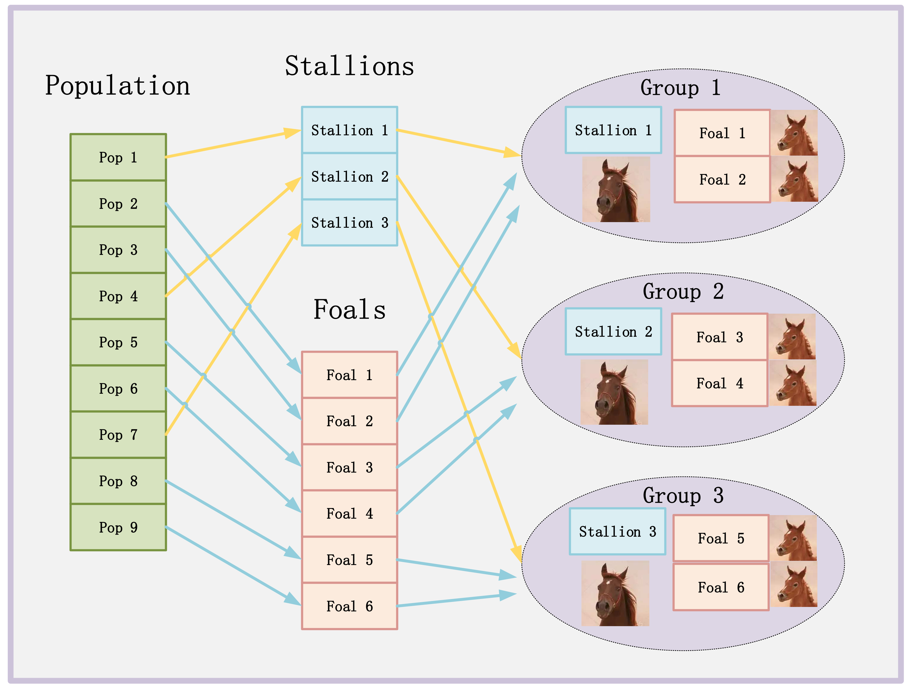
Generally, horses can be divided into two classes based on their social organization (territorial and non-territorial). They live in groups of different ages, such as offspring, stallions, and mares (see Figure 1). Both stallions and mares live together and interact with each other in grazing. Foals leave their groups after they grow up and join other groups to establish their own families. This behavior prevents mating between stallions and siblings.
The wild horse optimization (WHO) algorithm is a metaheuristic swarm-based algorithm inspired by the social behavior of horses, such as grazing, domination, leadership hierarchy, and mating.
The WHO algorithm consists of five different steps, described below:
2.1. Creating Initial Populations, Horse Groups, Determining Leaders
If N individuals and G groups exist, then the number of non-leaders (mares and foals) is N–G, and the number of leaders is G. The proportion of stallions is defined as PS, which is G/N. Figure 1 shows how leaders are determined from the basic generation to create various groups.
2.2. Grazing Behavior
As stated previously, most of a foal’s life is spent grazing near its group. In order to simulate the grazing phase, we assume that the stallion position existed in the grazing area center. The following formula is used to enable other individuals to move.
where and StallionG,j are the positions of the ith group member and stallion in the jth group, respectively, R is a random number between −2 and 2, and Z is an adaptive parameter computed by Equation (2):
where P is a vector containing 0 and 1, and its dimension equals the dimension of the problem, and are random vectors between 0 and 1, and R2 is a random number between 0 and 1. TDR is a linearly decreasing parameter computed by Equation (3).
where t and T are the current and maximum iterations, respectively.
2.3. Horse Mating Behavior
As stated previously, one of the unique behaviors of horses compared to other animals is separating foals from their original groups prior to their reaching puberty and mating. To be able to simulate the behavior of mating between horses, the following formula is used:
where is the position of horse p in group k, which is formed by positions of horse q in group i and horse z in group j. In the basic WHO, the probability of crossover is set to a constant named PC.
2.4. Group Leadership
Group leaders (stallions) will lead other group members to a suitable area (waterhole). Group leaders (stallions) will also compete for the waterhole, leading the dominant group to employ the waterhole first. The following formula is used to simulate this behavior:
where and StallionG,j are the candidate position and the current leader position in the jth group, respectively, and WH is the position of the waterhole.
2.5. Exchange and Selection of Leaders
At first, leaders are selected randomly. After that, leaders are selected based on their fitness values. To simulate the exchange between leader positions and other individuals, the following formula is used:
where f() and f(StallionG,j) are the fitness values of foal and stallion, respectively.
3. Improved Wild Horse Optimizer
In this section, the IWHO is introduced in detail. To enhance the optimizing capability of the basic algorithm, three methods are added. Firstly, wild horses in nature tend to chase and run. Thus, a random running strategy is applied to the foals and stallions. Then, a dynamic inertia weight strategy is introduced to the waterhole, which is from DSCA [50] and beneficial to balance exploration and exploitation. At last, the competition for waterhole mechanism is proposed for stallions, which is inspired by artificial gorilla troops optimizer (GTO) [57] and further improves the solution quality.
3.1. Random Running Strategy (RRS)
In nature, wild horses are very fond of running or chasing each other. Inspired by this, the random running strategy is proposed for both foals and stallions. The position-updating formula is presented as follow:
where lb and ub are the lower boundary and upper boundary, respectively.
When conducting the RRS, search agents may appear anywhere in the search space. Thus, this method can help search agents jump out of the local optima. Note that to balance exploration and exploitation, the probability of random running (PRR) is set to a small value of 0.1.
3.2. Dynamic Inertia Weight Strategy (DIWS)
The dynamic weight strategy has been applied in much research [55,58,59] and is helpful to find the optimal global solution when introduced into algorithms. Thus, to help the stallions find a better waterhole, a dynamic inertia weight is added to the waterhole in the first formula of Equation (5). The weight and modified formula are calculated as follows:
where wmin and wmax are the upper and lower boundary values, respectively, f(t)i is the fitness value of the current stallion at tth iteration, f(t)avg is the average fitness value of all stallions, and f(t)min is the minimum fitness value of the population.
3.3. Competition for Waterhole Mechanism (CWHM)
Moreover, the waterhole can be found by two stallions simultaneously. Then there may be rivalry between stallions over the waterhole. Thus, to further improve the solution quality, the competition for the waterhole mechanism, which is similar to the competition for adult females in GTO [53], is proposed to replace the second formula of Equation (5). The position updating formula is as follows:
where Q1 and Q2 are random numbers between −1 and 1.
3.4. Improved Wild Horse Optimizer
By combining the DIWS and CWHM, the following formula is used to replace Equation (5) in WHO:
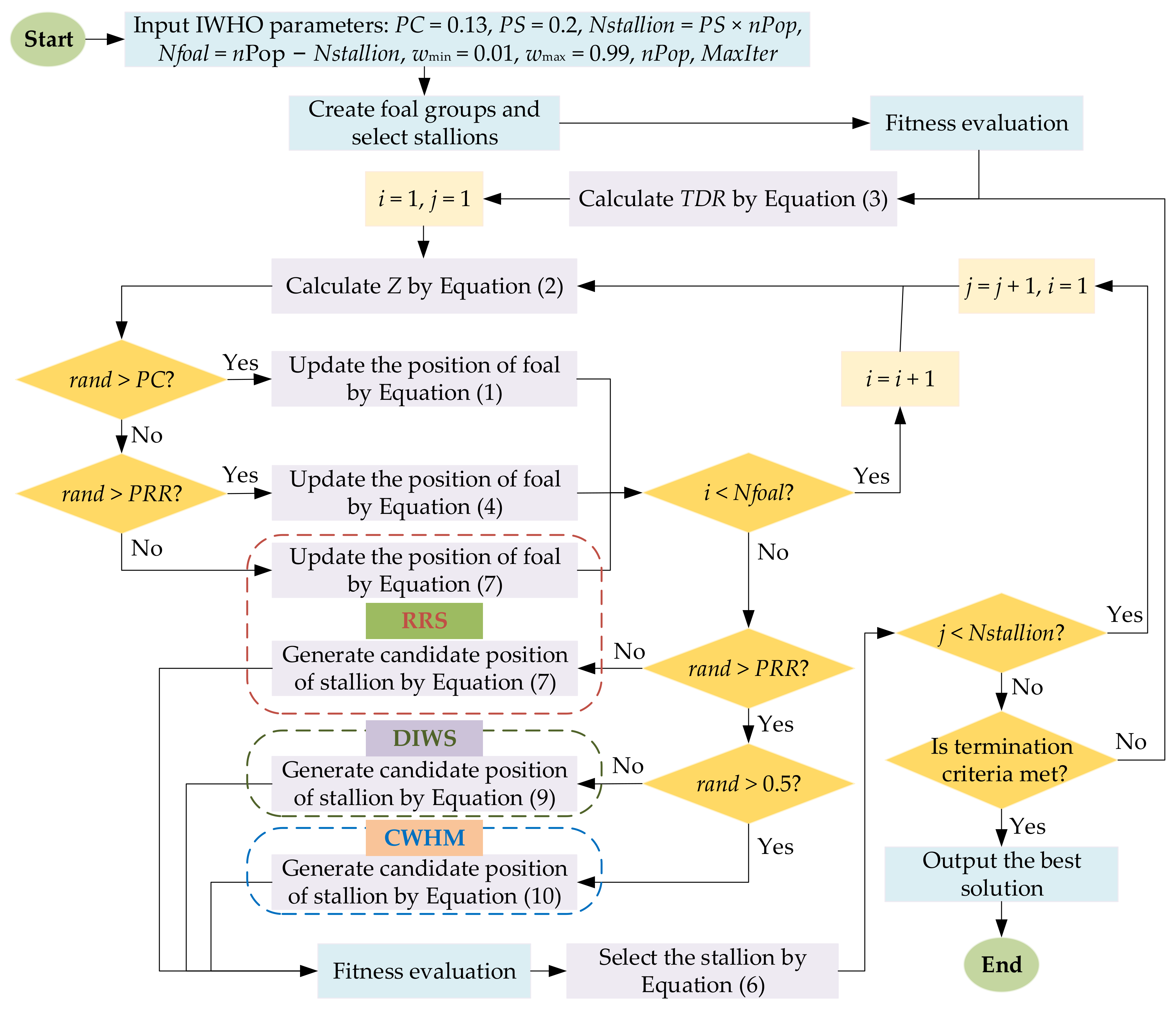
In IWHO, foals and stallions have a more flexible method to update their positions. The RRS helps search agents achieve a better balance between exploration and exploitation. At the same time, DIWS and CWHM enable the method to obtain high-quality solutions and improve the convergence speed. The pseudocode of IWHO is shown in Algorithm 1, and the flowchart of the proposed IWHO is shown in Figure 2.
| Algorithm 1 Pseudocode of IWHO |
| Start IWHO. 1. Input IWHO parameters: PC = 0.13, PS = 0.2, wmin = 0.01, wmax = 0.99, PRR = 0.1. 2. Set population size (N) and the maximum number of iterations (T). 3. Initialize the population of horses at random. 4. Create foal groups and select stallions. 5. While (t ≤ T) 6. Calculate TDR using Equation (3). 7. Calculate Z using Equation (2). 8. For the number of stallions 9. For the number of foals 10. If rand > PC 11. Update the position of the foal using Equation (1). 12. Else if rand > PRR 13. Update the position of the foal using Equation (4). 14. Else 15. Update the position of the foal using Equation (7). 16. End 17. End for 18. If rand > PRR 19. If rand > 0.5 20. Generate the candidate position of stallion using Equation (10). 21. Else 22. Generate the candidate position of stallion using Equation (9). 23. End if 24. Else 25. Generate the candidate position of stallion using Equation (7). 26. End if 27. If the candidate position of the stallion is better 28. Replace the position of the stallion using the candidate position. 29. End if 30. End for 31. Exchange foals and stallions position using Equation (6). 32. t = t + 1 33. End While 34. Output the best solution obtained by IWHO. End IWHO. |
3.5. Analysis of Algorithm Computational Complexity
The computational complexity of IWHO is related to the population size (N), the maximum number of iterations (T), and problem dimensions (D). In the basic WHO, the computational complexity of initializing population is O(N × D). Then, the computational complexity of updating positions for foals and stallions is O(N × D × T). In addition, consider the worst-case scenario: all foals conduct the grazing behavior. The computational complexity of calculating Z is O(N × D × T). The computational complexity of the exchange and selection of leaders is O(Nfoal × T). Thus, the overall computational complexity of WHO is O(2 × N × D × T + N × D + Nfoal × T). In IWHO, it should be noted that the proposed RRS and CWHM would not increase the computational complexity.
Similarly, considering the worst-case scenario, all stallions conduct the DIWS. Then, the computational complexity of calculating weight is O(Nstallion × T). Therefore, the overall computational complexity of IWHO is O(2 × N × D × T + N × D + N × T), which is only a little higher than the basic algorithm.
4. Experimental Study
To be able to show the significant performance and superiority of IWHO, a variety of experiments were carried out. IWHO was tested over 33 mathematical functions taken from two well-known benchmark function datasets: CEC2005 [60] and CEC2021 [61]. IWHO performance was compared to classical WHO and eight different algorithms. The parameter settings of these experiments are discussed in the following subsection.
4.1. Optimization of Functions and Parameter Settings
Thirty-three mathematical functions of different types (unimodal, multimodal, fixed-dimension multimodal functions) were implemented from two different benchmark datasets: CEC2005 and CEC2021. Table 1 shows each mathematical function used to carry out these experiments, including its type, range of the search space, and its global optimal value.
IWHO has been compared to WHO and eight other algorithms: grey wolf optimizer (GWO) [50], moth–flame optimization (MFO) [51], salp swarm algorithm (SSA) [52], whale optimization algorithm (WOA) [53], particle swarm optimizer (PSO) [15], hybrid sine–cosine algorithm with harmony search (HSCAHS) [54], dynamic sine–cosine algorithm (DSCA) [55], and modified ant lion optimizer (MALO) [56]. The parameter settings of each algorithm are shown in Table 2. These comparative algorithms have shown certain optimizing capability to the benchmark functions. However, for some optimization problems, they cannot get satisfactory optimization solutions. Hence, the advantages of the improved algorithm can be revealed through the extensive comparison between the improved algorithm and other algorithms.
The experiments were carried out in Windows 10 with 16 GB RAM and an Intel (R) i5-9500 CPU. All simulations were executed using MATLAB R2016a. Moreover, the maximum number of iterations was set at 500, and the number of individuals was set to 30. In contrast, the number of dimensions was different according to each function, as shown in Table 1.
4.2. Analysis of Performance for the CEC 2005 Test Suite
Improved WHO (IWHO) results with other comparative algorithms are listed in Table 3. This table shows that the suggested approach achieves the best results in almost all unimodal functions (F1–F7) in all mentioned dimensions (30, 200, 500, and 1000). On the other hand, IWHO also ranked first in almost multimodal functions (F8–F13), and in almost functions regarding fixed-dimension multimodal functions (F14–F23). Compared to basic WHO and other algorithms, it can be seen that the improved algorithm has better exploration and exploitation capability as a result of the three improvements.
Moreover, a non-parametric test known as Wilcoxon signed test was used to give evidence of the performance of our suggested approach. Table 4 shows the Wilcoxon results of IWHO vs. other algorithms with 5% significance [62]. From this table, we can see that IWHO is better than many other metaheuristics algorithms in most cases.
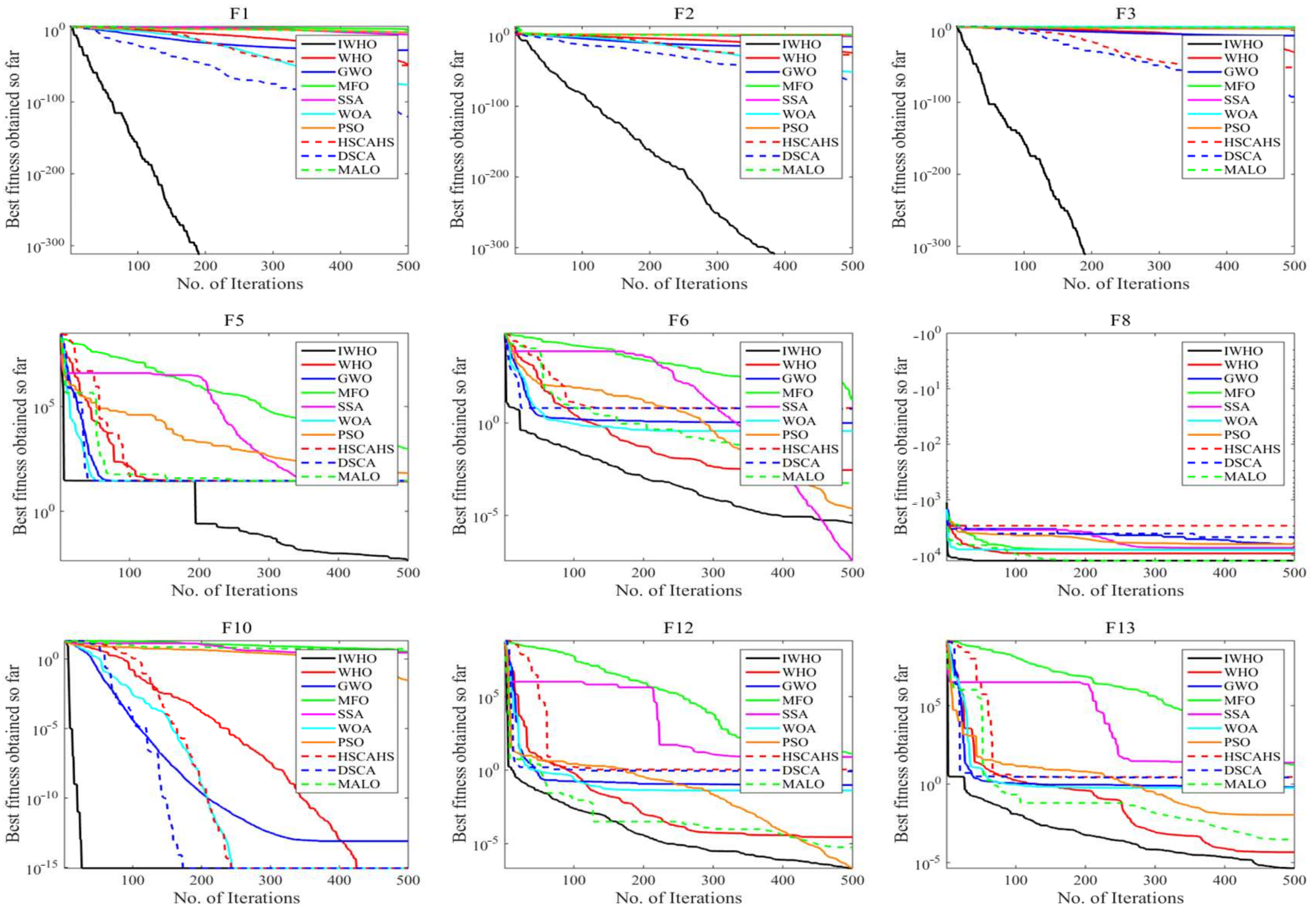
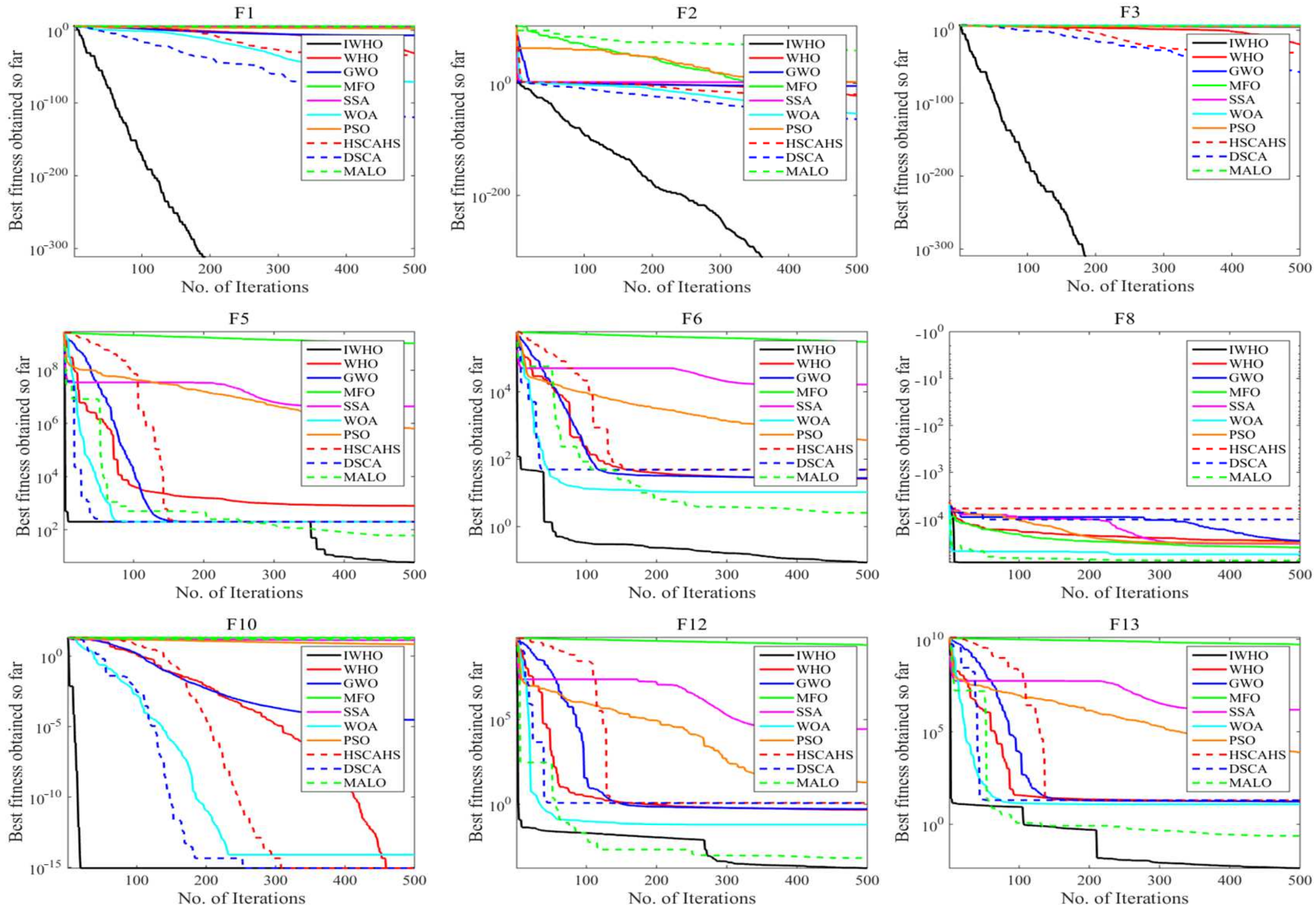
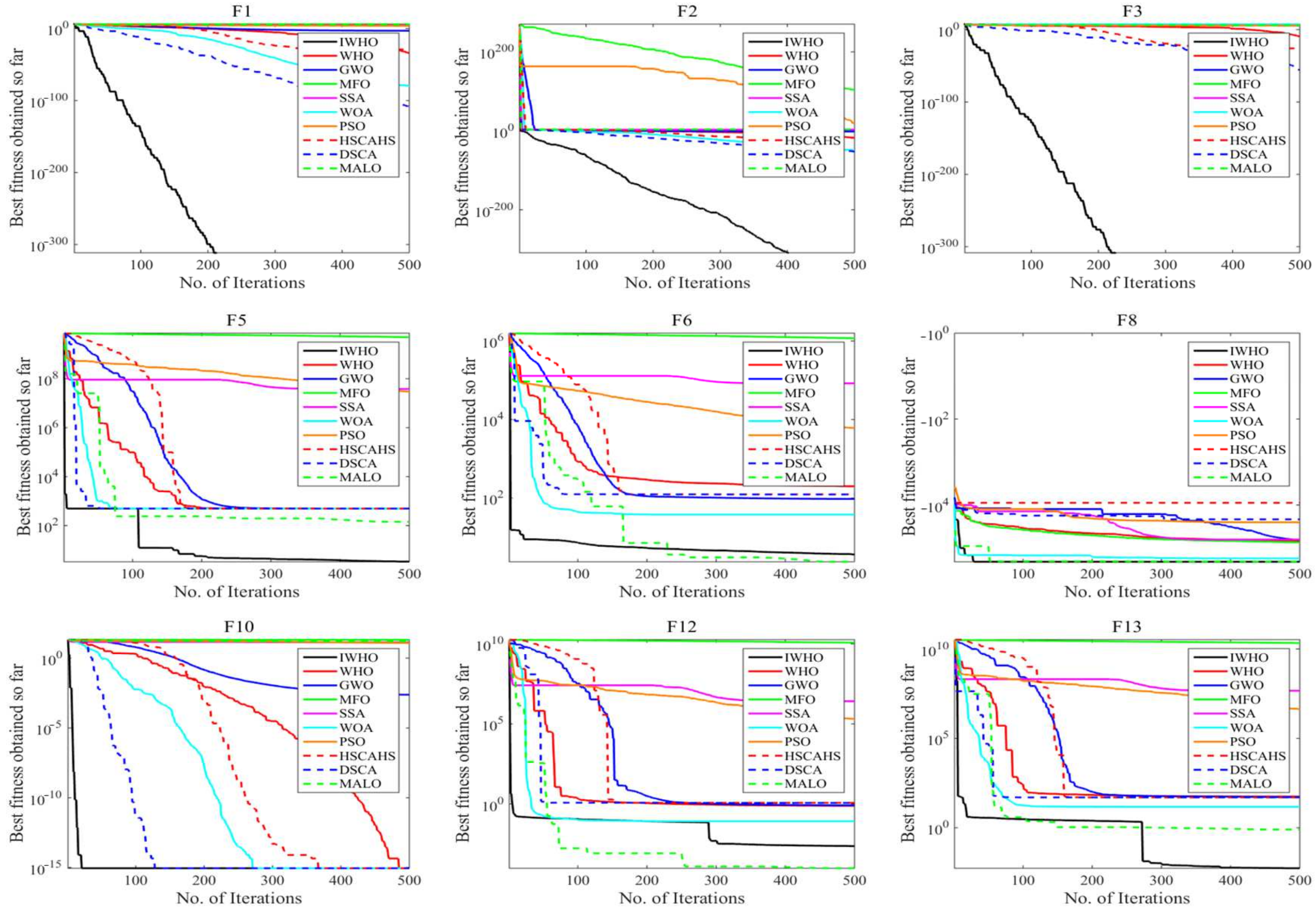
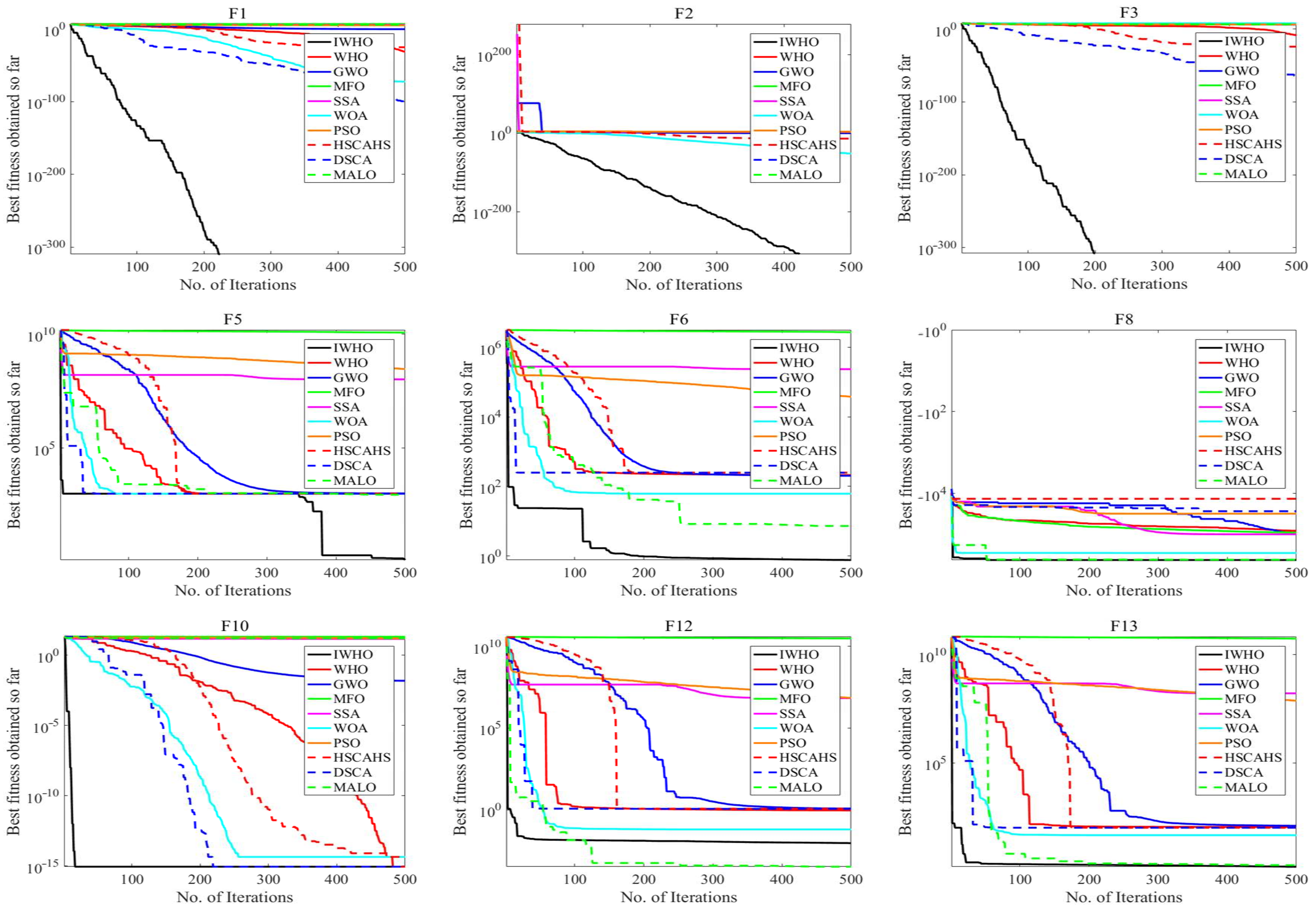
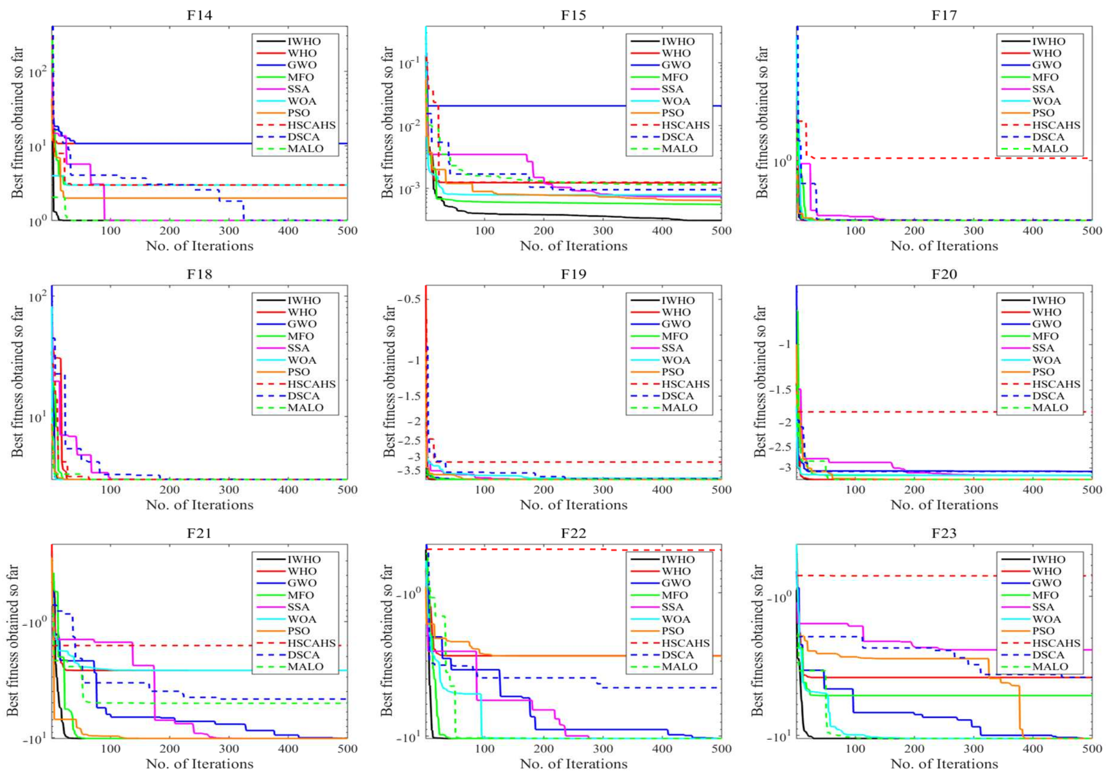
Furthermore, Figure 3 shows the convergence curves of some functions (F1–F3, F5, F6, F8, F10, F12, F13) with 30 dimensions. It is clear from this figure that IWHO has powerful convergence. Further, Figure 4, Figure 5 and Figure 6 show the convergence curves of the same functions (F1–F3, F5, F6, F8, F10, F12, F13) with dimensions of 200, 500, and 1000, respectively. Figure 7 shows the convergence curves for some fixed-dimension multimodal functions (F14, F15, F17–F23). It is obvious that the suggested algorithm has good convergence even in these multimodal functions.
4.3. Statistical Analysis of Performance for the CEC 2021 Test Suite
In this subsection, the performance of IWHO is tested using ten mathematical functions from IEEE CEC 2021, and it is compared using the same comparative metaheuristics algorithms.
The results of CEC2021 test functions are given in Table 5 in terms of mean and standard deviation. Table 5 also shows the results of Friedman ranking test [63]. It can be seen that the proposed IWHO is ranked first in CEC_02 and CEC_06 and the second-best in the other two functions (CEC_05 and CEC_08). Overall, it is also ranked first.
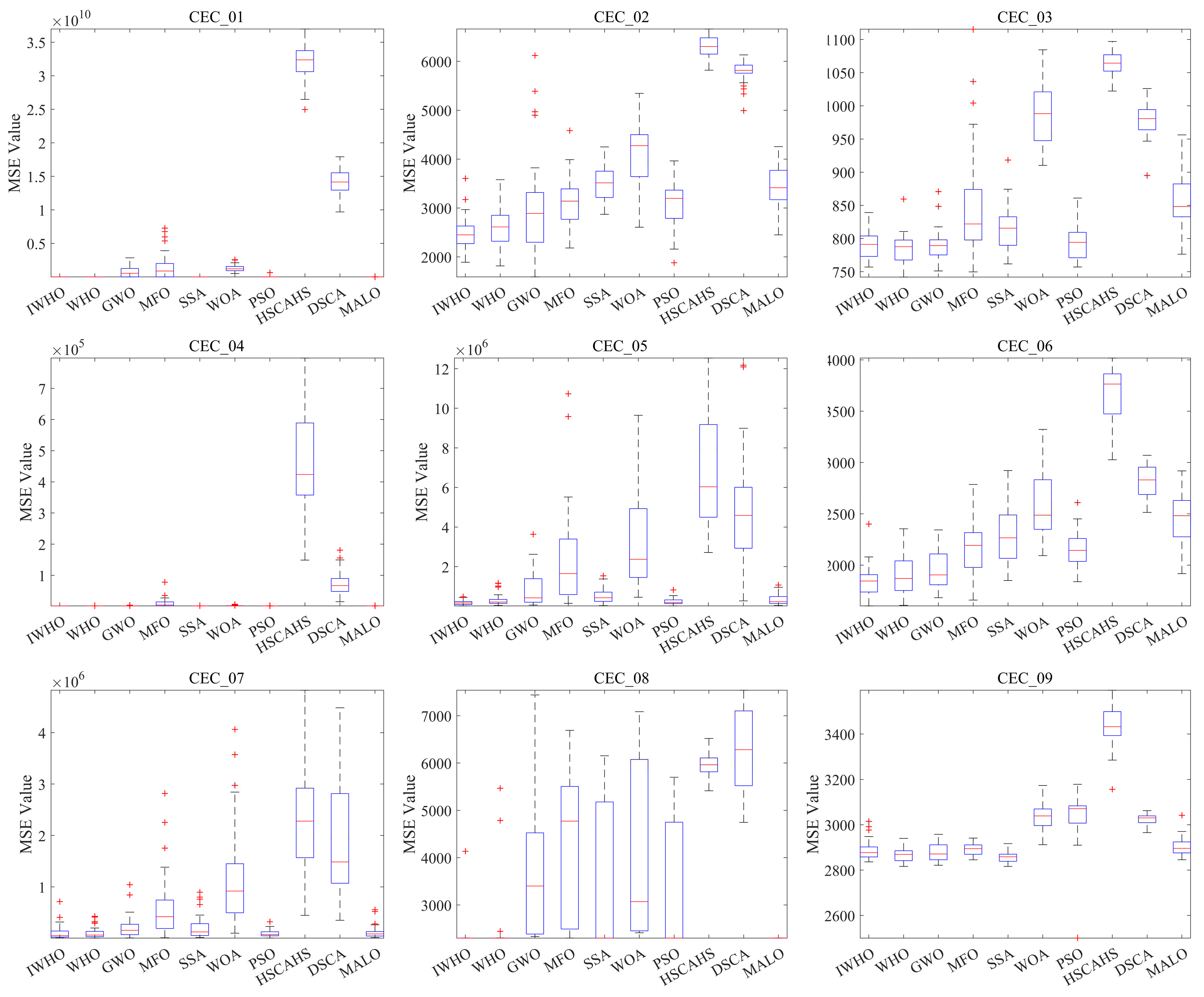
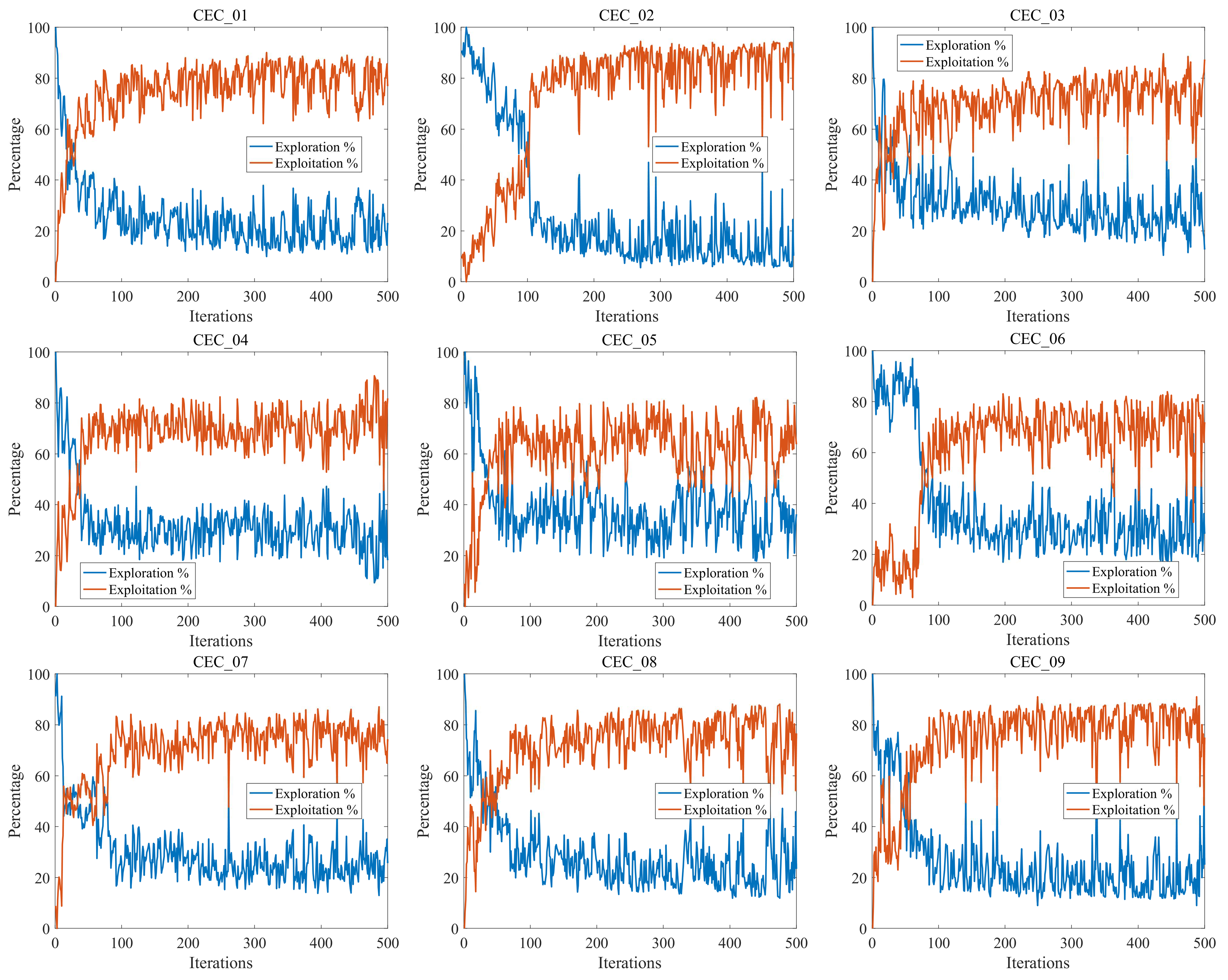
Figure 8 shows the box plots of the introduced algorithm and other compared ones using nine functions (CEC_01–CEC_09). It can be seen that the improved algorithm has better stability in these functions. Further, Figure 9 shows different exploration and exploitation phases. The percentages of exploration and exploitation phases are calculated based on the dispersion of all searching individuals, which exhibits the flexibility of improved algorithms during the optimization process.
5. Real-World Applications
In this section, several real-world engineering design problems with constraints are utilized to assess IWHO’s significance and effectiveness. IWHO has been evaluated using five engineering design problems: welded beam, tension/compression spring, three-bar truss, car crashworthiness, and speed reducer design problems.
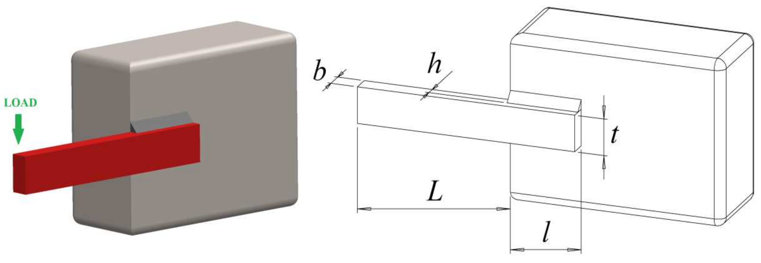
5.1. Welded Beam Design Problem
The first engineering problem used to evaluate IWHO is the welded beam design, a common and well-known problem [64], as shown in Figure 10. Welded beam aims to select the optimal variables to decrease the entire weld beam manufacturing cost subject to:
- Welded thickness (h)
- Bar length (l)
- Bar height (t)
- Bar thickness (b)
The mathematical equations of this problem are shown below:
Consider:
Minimize:
Subject to:
where:
Range of variables:
IWHO has been compared to the original WHO [49], GWO [50], MFO [51], WOA [53], SCA [65], ALO [66], DA [67], and LSHADE [68]. From Table 6, it’s obvious that IWHO achieves the best results compared to other algorithms. It achieves [h, l, t, b] = [0.2057, 3.2530, 9.0366, 0.2057] with fitness value 1.6952.
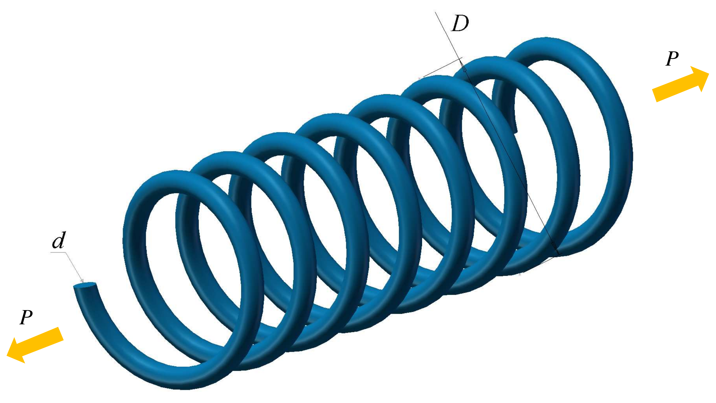
5.2. Tension/Compression Spring Design Problem
The second constrained problem is the tension/compression spring problem [69], the goal of which is to select the optimal parameters to minimize the price of manufacturing a spring, as shown in Figure 11. This problem has three variables:
- Diameter of wire (d)
- Coil diameter (D)
- Active coils number (N)
The mathematical description of this problem is given below:
Consider:
Minimize:
Subject to:
Range of variables:
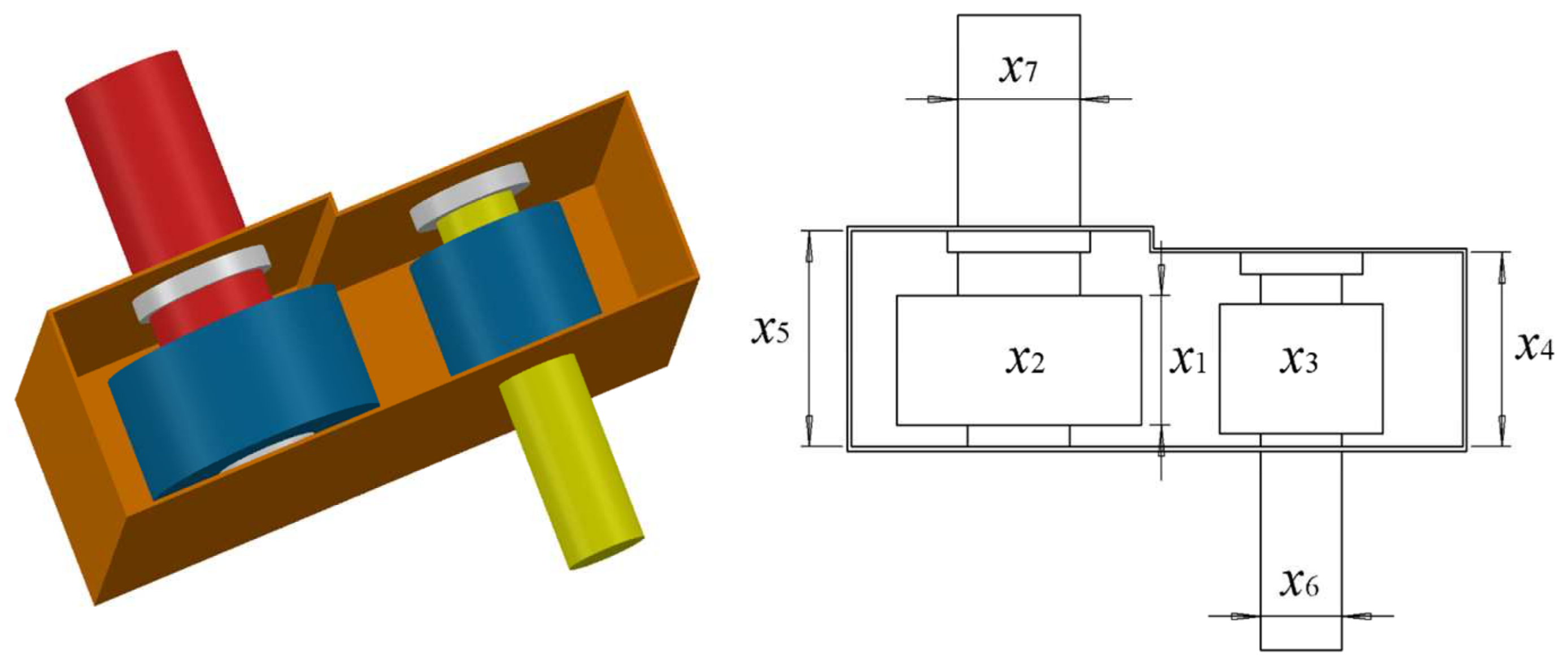
5.3. Three-Bar Truss Design Problem
This engineering problem is a non-linear optimization problem introduced by Nowcki to minimize bar structure burdens [74]. Three-bar truss has two variables, as shown in Figure 12. The mathematical description of this problem is given below:
Consider:
Minimize:
Subject to:
where:
Range of variables:
The results of this problem are given in Table 8, comparing IWHO with basic WHO [49], HHO [71], SSA [52], AOA [75], MVO [72], MFO [51], and GOA [18]. IWHO achieves the best solution [x1, x2] = [0.7884, 0.4081] and its objective value is 263.8523.

Table 8.
Optimization results for the three-bar truss design problem.
| Algorithm | Optimal Values for Variables | Optimum Weight | |
|---|---|---|---|
| x1 | x2 | ||
| IWHO | 0.7884 | 0.4081 | 263.8523 |
| WHO [49] | 0.7980 | 0.3816 | 263.9181 |
| HHO [71] | 0.788662816 | 0.408283133832900 | 263.8958434 |
| SSA [52] | 0.78866541 | 0.408275784 | 263.89584 |
| AOA [75] | 0.79369 | 0.39426 | 263.9154 |
| MVO [72] | 0.78860276 | 0.408453070000000 | 263.8958499 |
| MFO [51] | 0.788244771 | 0.409466905784741 | 263.8959797 |
| GOA [18] | 0.788897555578973 | 0.407619570115153 | 263.895881496069 |
5.4. Car Crashworthiness Design Problem
The car crashworthiness problem was first introduced by Gu et al. [76]. This engineering problem has 10 constraints and 11 design variables. The mathematical description and 3D model diagram of this problem can be seen in [77].
The results of this problem are given in Table 9, where IWHO is compared to GWO [50], GOA [18], PSO [15], MFO [51], SSA [52], DSCA [55], MALO [56]. From this table, we can conclude that IWHO achieves the best results [x1 − x11] = [0.5000, 1.1186, 0.5000, 1.2982, 0.5000, 1.5000, 0.5000, 0.3450, 0.3450, −19.1594, 0.0020] with fitness value 22.8427.
5.5. Speed Reducer Design Problem
The last constrained engineering problem is the speed reducer design problem [75], as shown in Figure 13, which aims to find the minimum weight of the speed reducer. This problem has seven variables. The mathematical formulation of this problem is shown below:
Minimize:
Subject to:
Range of variables:
6. Conclusions
In this paper, an improved wild horse optimizer (IWHO) is proposed for solving global optimization problems. The basic WHO is enhanced by integrating three improvements: random running strategy (RRS), dynamic inertia weight strategy (DIWS), and competition for waterhole mechanism (CWHM), which were inspired by the behavior of wild horses. RRS is utilized to enhance the global search capability and balance exploration and exploitation, while DIWS and CWHM are applied to increase the quality of the optimal solution. To evaluate the performance of the proposed IWHO, twenty-three classical benchmark functions with various types and dimensions, ten CEC 2021 test functions, and five real-world optimization problems are employed for testing. Meanwhile, nine well-known algorithms are used for comparison: basic wild horse optimizer (WHO), grey wolf optimizer (GWO), moth–flame optimization (MFO), salp swarm algorithm (SSA), whale optimization algorithm (WOA), particle swarm optimizer (PSO), hybridizing sine–cosine algorithm with harmony search (HSCAHS), dynamic sine–cosine algorithm (DSCA), and modified ant lion optimizer (MALO). The numerical and statistical results indicate that IWHO outperforms other methods for most test functions, showing that the improvements applied to WHO are successful. In addition, the results of engineering design problems verify the applicability of the proposed IWHO.
In the future, IWHO may be applied to high-dimensional, real-world problems, such as multilayer perceptron training for solving classification tasks. Additionally, the IWHO can be hybridized with other metaheuristic algorithms to further improve its optimization capability and solve more optimization problems, such as feature selection, multilevel thresholding image segmentation, and parameter optimization.
Author Contributions
Conceptualization, R.Z.; methodology, R.Z. and H.-M.J.; software, S.W.; validation, D.W.; writing—original draft preparation, A.G.H. and R.Z.; writing—review and editing, L.A. and H.-M.J.; funding acquisition, R.Z. and H.-M.J. All authors have read and agreed to the published version of the manuscript.
Funding
This work was funded by Sanming University, which introduces high-level talent to start scientific research; funding support project (21YG01, 20YG14), Sanming University National Natural Science Foundation Breeding Project (PYT2103, PYT2105), Fujian Natural Science Foundation Project (2021J011128), Guiding Science and Technology Projects in Sanming City (2021-S-8), Educational Research Projects of Young and Middle-Aged Teachers in Fujian Province (JAT200618), Scientific Research and Development Fund of Sanming University (B202009), and by Open Research Fund Program of Fujian Provincial Key Laboratory of Agriculture Internet of Things Application (ZD2101).
Institutional Review Board Statement
Not applicable.
Informed Consent Statement
Not applicable.
Acknowledgments
The authors would like to thank the support of Fujian Key Lab of Agriculture IoT Application and IoT Application Engineering Research Center of Fujian Province Colleges and Universities, and also the anonymous reviewers and the editor for their careful reviews and constructive suggestions to help us improve the quality of this paper.
Conflicts of Interest
The authors declare that they have no conflict of interest.
References
- Hassanien, A.E.; Emary, E. Swarm Intelligence: Principles, Advances, and Applications; CRC Press: Boca Raton, FL, USA, 2018; pp. 93–119. [Google Scholar]
- Hussien, A.G.; Hassanien, A.E.; Houssein, E.H.; Amin, M.; Azar, A.T. New binary whale optimization algorithm for discrete optimization problems. Eng. Optimiz. 2020, 52, 945–959. [Google Scholar] [CrossRef]
- Yang, X.S. Engineering Optimization: An Introduction with Metaheuristic Applications; John Wiley & Sons: Hoboken, NJ, USA, 2010. [Google Scholar]
- Jamil, M.; Yang, X.S. A literature survey of benchmark functions for global optimization problems. Int. J. Math. Model. Numer. Optim. 2013, 4, 150–194. [Google Scholar]
- Fathi, H.; AlSalman, H.; Gumaei, A.; Manhrawy, I.I.M.; Hussien, A.G.; El-Kafrawy, P. An Efficient Cancer Classification Model Using Microarray and High-Dimensional Data. Comput. Intel. Neurosc. 2021, 2021, 7231126. [Google Scholar] [CrossRef] [PubMed]
- Mousavi-Avval, S.H.; Rafiee, S.; Sharifi, M.; Hosseinpour, S.; Notarnicola, B.; Tassielli, G.; Renzulli, P.A. Application of multi-objective genetic algorithms for optimization of energy, economics and environmental life cycle assessment in oilseed production. J. Clean. Prod. 2017, 140, 804–815. [Google Scholar] [CrossRef]
- Abualigah, L.; Gandomi, A.H.; Elaziz, M.A.; Hussien, A.G.; Khasawneh, A.M.; Alshinwan, M.; Houssein, E.H. Nature-inspired optimization algorithms for text document clustering—A comprehensive analysis. Algorithms 2020, 13, 345. [Google Scholar] [CrossRef]
- Shamir, J.; Rosen, J.; Mahlab, U.; Caulfield, H.J. Optimization methods for pattern recognition. Int. Soc. Opt. Eng. 1992, 40, 2–24. [Google Scholar]
- Houssein, E.H.; Amin, M.; Hassanien, A.G.; Houssein, A.E. Swarming behaviour of salps algorithm for predicting chemical compound activities. In Proceedings of the 8th IEEE International Conference on Intelligent Computing and Information Systems (ICICIS), Cairo, Egypt, 5–7 December 2017; pp. 315–320. [Google Scholar]
- Chou, J.S.; Pham, A.D. Nature-inspired metaheuristic optimization in least squares support vector regression for obtaining bridge scour information. Inform. Sci. 2017, 399, 64–80. [Google Scholar] [CrossRef]
- Hussien, A.G.; Hassanien, A.E.; Houssein, E.H.; Bhattacharyya, S.; Amin, M. S-shaped Binary Whale Optimization Algorithm for Feature Selection. In Recent Trends in Signal and Image Processing; Springer: Singapore, 2019; Volume 727, pp. 79–87. [Google Scholar]
- Hussien, A.G.; Houssein, E.H.; Hassanien, A.E. A binary whale optimization algorithm with hyperbolic tangent fitness function for feature selection. In Proceedings of the 8th IEEE International Conference on Intelligent Computing and Information Systems (ICICIS), Cairo, Egypt, 5–7 December 2017; pp. 166–172. [Google Scholar]
- Besnassi, M.; Neggaz, N.; Benyettou, A. Face detection based on evolutionary Haar filter. Pattern Anal. Appl. 2020, 23, 309–330. [Google Scholar] [CrossRef]
- Wang, Z.Y.; Xing, H.L.; Li, T.R.; Yang, Y.; Qu, R.; Pan, Y. A modified ant colony optimization algorithm for network coding resource minimization. IEEE T. Evolut. Comput. 2016, 20, 325–342. [Google Scholar] [CrossRef] [Green Version]
- Kennedy, J.; Eberhart, R. Particle swarm optimization. In Proceedings of the IEEE International Conference on Neural Networks, Perth, Australia, 27 November–1 December 1995; pp. 1942–1948. [Google Scholar]
- Dorigo, M.; Gambardella, L.M. Ant colony system: A cooperative learning approach to the traveling salesman problem. IEEE T. Evolut. Comput. 1997, 1, 53–66. [Google Scholar] [CrossRef] [Green Version]
- Yang, X.S.; Deb, S. Cuckoo search via Lévy flights. In Proceedings of the World Congress on Nature & Biologically Inspired Computing (NaBIC), Coimbatore, India, 9–11 December 2009; pp. 210–214. [Google Scholar]
- Saremi, S.; Mirjalili, S.; Lewis, A. Grasshopper optimisation algorithm: Theory and application. Adv. Eng. Softw. 2017, 105, 30–47. [Google Scholar] [CrossRef] [Green Version]
- Li, M.D.; Zhao, H.; Weng, X.W.; Han, T. A novel nature-inspired algorithm for optimization: Virus colony search. Adv. Eng. Softw. 2016, 92, 65–88. [Google Scholar] [CrossRef]
- Kaveh, A.; Farhoudi, N. A new optimization method: Dolphin echolocation. Adv. Eng. Softw. 2013, 59, 53–70. [Google Scholar] [CrossRef]
- Hussien, A.G.; Amin, M. A self-adaptive Harris Hawks optimization algorithm with opposition-based learning and chaotic local search strategy for global optimization and feature selection. Int. J. Mach. Learn. Cyb. 2022, 13, 309–336. [Google Scholar] [CrossRef]
- Hussien, A.G.; Oliva, D.; Houssein, E.H.; Juan, A.A.; Yu, X. Binary whale optimization algorithm for dimensionality reduction. Mathematics 2020, 8, 1821. [Google Scholar] [CrossRef]
- Assiri, A.S.; Hussien, A.G.; Amin, M. Ant Lion Optimization: Variants, hybrids, and applications. IEEE Access 2020, 8, 77746–77764. [Google Scholar] [CrossRef]
- Hussien, A.G.; Amin, M.; Wang, M.; Liang, G.; Alsanad, A.; Gumaei, A.; Chen, H. Crow Search Algorithm: Theory, Recent Advances, and Applications. IEEE Access 2020, 8, 173548–173565. [Google Scholar] [CrossRef]
- Hussien, A.G. An enhanced opposition-based Salp Swarm Algorithm for global optimization and engineering problems. J. Amb. Intel. Hum. Comp. 2021, 13, 129–150. [Google Scholar] [CrossRef]
- Hussien, A.G.; Amin, M.; Abd El Aziz, M. A comprehensive review of moth-flame optimisation: Variants, hybrids, and applications. J. Exp. Theor. Artif. Intell. 2020, 32, 705–725. [Google Scholar] [CrossRef]
- Hashim, F.A.; Hussien, A.G. Snake Optimizer: A novel meta-heuristic optimization Algorithm. Knowl.-Based Syst. 2022, 242, 108320. [Google Scholar] [CrossRef]
- Mostafa, R.R.; Hussien, A.G.; Khan, M.A.; Kadry, S.; Hashim, F. Enhanced COOT Optimization Algorithm for Dimensionality Reduction. In Proceedings of the Fifth International Conference of Women in Data Science at Prince Sultan University (WiDS PSU), Riyadh, Saudi Arabia, 28–29 March 2022. [Google Scholar] [CrossRef]
- Jain, M.; Singh, V.; Rani, A. A novel nature-inspired algorithm for optimization: Squirrel search algorithm. Swarm Evol. Comput. 2019, 44, 148–175. [Google Scholar] [CrossRef]
- Holland, J.H. Adaptation in Natural and Artificial Systems: An Introductory Analysis with Applications to Biology, Control, and Artificial Intelligence; MIT Press: Cambridge, MA, USA, 1992. [Google Scholar]
- Juste, K.; Kita, H.; Tanaka, E.; Hasegawa, J. An evolutionary programming solution to the unit commitment problem. IEEE T. Power Syst. 1999, 14, 1452–1459. [Google Scholar] [CrossRef]
- Rocca, P.; Oliveri, G.; Massa, A. Differential evolution as applied to electromagnetics. IEEE Antennas Propag. Mag. 2011, 53, 38–49. [Google Scholar] [CrossRef]
- Passino, K.M. Biomimicry of bacterial foraging for distributed optimization and control. IEEE Contr. Syst. Mag. 2002, 22, 52–67. [Google Scholar]
- Moscato, P.; Mendes, A.; Berretta, R. Benchmarking a memetic algorithm for ordering microarray data. Biosystems 2007, 88, 56–75. [Google Scholar] [CrossRef] [PubMed]
- Kirkpatrick, S.; Gelatt, C.D., Jr.; Vecchi, M.P. Optimization by simulated annealing. Science 1983, 220, 671–680. [Google Scholar] [CrossRef] [PubMed]
- Rashedi, E.; Nezamabadi-Pour, H.; Saryazdi, S. GSA: A gravitational search algorithm. Inform. Sci. 2009, 179, 2232–2248. [Google Scholar] [CrossRef]
- BİRBİL, Ş.İ.; Fang, S.C. An electromagnetism-like mechanism for global optimization. J. Glob. Optim. 2003, 25, 263–282. [Google Scholar] [CrossRef]
- Javidy, B.; Hatamlou, A.; Mirjalili, S. Ions motion algorithm for solving optimization problems. Appl. Soft Comput. 2015, 32, 72–79. [Google Scholar] [CrossRef]
- Abualigah, L.; Abd Elaziz, M.; Hussien, A.G.; Alsalibi, B.; Jalali, S.M.J.; Gandomi, A.H. Lightning search algorithm: A comprehensive survey. Appl. Intell. 2021, 51, 2353–2376. [Google Scholar] [CrossRef]
- Doğan, B.; Ölmez, T. A new metaheuristic for numerical function optimization: Vortex search algorithm. Inform. Sci. 2015, 293, 125–145. [Google Scholar] [CrossRef]
- Rao, R.V.; Savsani, V.J.; Vakharia, D. Teaching–learning-based optimization: A novel method for constrained mechanical design optimization problems. Comput. Aided Des. 2011, 43, 303–315. [Google Scholar] [CrossRef]
- Atashpaz-Gargari, E.; Lucas, C. Imperialist competitive algorithm: An algorithm for optimization inspired by imperialistic competition. In Proceedings of the IEEE Congress on Evolutionary Computation, Singapore, 25–28 September 2007; pp. 4661–4667. [Google Scholar]
- Ramezani, F.; Lotfi, S. Social-based algorithm (SBA). Appl. Soft Comput. 2013, 13, 2837–2856. [Google Scholar] [CrossRef]
- Wolpert, D.H.; Macready, W.G. No free lunch theorems for optimization. IEEE T. Evolut. Comput. 1997, 1, 67–82. [Google Scholar] [CrossRef] [Green Version]
- Ning, G.Y.; Cao, D.Q. Improved Whale Optimization Algorithm for Solving Constrained Optimization Problems. Discret. Dyn. Nat. Soc. 2021, 2021, 8832251. [Google Scholar] [CrossRef]
- Nautiyal, B.; Prakash, R.; Vimal, V.; Liang, G.; Chen, H. Improved Salp Swarm Algorithm with Mutation Schemes for Solving Global Optimization and Engineering Problems. Eng. Comput. 2021, 1–23. [Google Scholar] [CrossRef]
- Tubishat, M.; Idris, N.; Shuib, L.; Abushariah, M.A.M.; Mirjalili, S. Improved Salp Swarm Algorithm Based on Opposition Based Learning and Novel Local Search Algorithm for Feature Selection. Expert Syst. Appl. 2020, 145, 113122. [Google Scholar] [CrossRef]
- Pelusi, D.; Mascella, R.; Tallini, L.; Nayak, J.; Naik, B.; Deng, Y. An Improved Moth-Flame Optimization Algorithm with Hybrid Search Phase. Knowl. Based Syst. 2020, 191, 105277. [Google Scholar] [CrossRef]
- Naruei, I.; Keynia, F. Wild horse optimizer: A new meta-heuristic algorithm for solving engineering optimization problems. Eng. Comput. 2021. [Google Scholar] [CrossRef]
- Mirjalili, S.; Mirjalili, S.M.; Lewis, A. Grey wolf optimizer. Adv. Eng. Softw. 2014, 69, 46–61. [Google Scholar] [CrossRef] [Green Version]
- Mirjalili, S. Moth-flame optimization algorithm: A novel nature-inspired heuristic paradigm. Knowl. Based Syst. 2015, 89, 228–249. [Google Scholar] [CrossRef]
- Mirjalili, S.; Gandomi, A.H.; Mirjalili, S.Z.; Saremi, S.; Faris, H.; Mirjalili, S.M. Salp Swarm Algorithm: A bio-inspired optimizer for engineering design problems. Adv. Eng. Softw. 2017, 114, 163–191. [Google Scholar] [CrossRef]
- Mirjalili, S.; Lewis, A. The whale optimization algorithm. Adv. Eng. Softw. 2016, 95, 51–67. [Google Scholar] [CrossRef]
- Singh, N.; Kaur, J. Hybridizing sine-cosine algorithm with harmony search strategy for optimization design problems. Soft Comput. 2021, 25, 11053–11075. [Google Scholar] [CrossRef]
- Li, Y.; Zhao, Y.; Liu, J. Dynamic sine cosine algorithm for large-scale global optimization problems. Expert Syst. Appl. 2021, 177, 114950. [Google Scholar] [CrossRef]
- Wang, S.; Sun, K.; Zhang, W.; Jia, H. Multilevel thresholding using a modified ant lion optimizer with opposition-based learning for color image segmentation. Math. Biosci. Eng. 2021, 18, 3092–3143. [Google Scholar] [CrossRef]
- Abdollahzadeh, B.; Gharehchopogh, F.S.; Mirjalili, S. Artificial gorilla troops optimizer: A new nature-inspired metaheuristic algorithm for global optimization problems. Int. J. Intell. Syst. 2021, 36, 5887–5958. [Google Scholar] [CrossRef]
- Chen, H.L.; Yang, C.J.; Heidari, A.A.; Zhao, X.H. An efficient double adaptive random spare reinforced whale optimization algorithm. Expert Syst. Appl. 2020, 154, 113018. [Google Scholar] [CrossRef]
- Dong, H.; Xu, Y.L.; Li, X.P.; Yang, Z.L.; Zou, C.H. An improved antlion optimizer with dynamic random walk and dynamic opposite learning. Knowl. Based Syst. 2021, 216, 106752. [Google Scholar] [CrossRef]
- Suganthan, P.N.; Hansen, N.; Liang, J.J.; Deb, K.; Chen, Y.P.; Auger, A.; Tiwari, S. Problem Definitions and Evaluation Criteria for the CEC 2005 Special Session on Real-Parameter Optimization; Technical Report, Nanyang Technological University, Singapore and KanGAL; Kanpur Genetic Algorithms Lab.: Kanpur, India, 2005. [Google Scholar]
- Zheng, R.; Jia, H.M.; Abualigah, L.; Wang, S.; Wu, D. An improved remora optimization algorithm with autonomous foraging mechanism for global optimization problems. Math. Biosci. Eng. 2022, 19, 3994–4037. [Google Scholar] [CrossRef]
- García, S.; Fernández, A.; Luengo, J.; Herrera, F. Advanced nonparametric tests for multiple comparisons in the design of experiments in computational intelligence and data mining: Experimental analysis of power. Inf. Sci. 2010, 180, 2044–2064. [Google Scholar] [CrossRef]
- Theodorsson-Norheim, E. Friedman and Quade tests: BASIC computer program to perform nonparametric two-way analysis of variance and multiple comparisons on ranks of several related samples. Comput. Biol. Med. 1987, 17, 85–99. [Google Scholar] [CrossRef]
- Coello, C.A.C. Use of a self-adaptive penalty approach for engineering optimization problems. Comput. Ind. 2000, 41, 113–127. [Google Scholar] [CrossRef]
- Mirjalili, S. SCA: A sine cosine algorithm for solving optimization problems. Knowl. Based Syst. 2016, 96, 120–133. [Google Scholar] [CrossRef]
- Mirjalili, S. The ant lion optimizer. Adv. Eng. Softw. 2015, 83, 80–98. [Google Scholar] [CrossRef]
- Mirjalili, S. Dragonfly algorithm: A new meta-heuristic optimization technique for solving single-objective, discrete, and multi-objective problems. Neural Comput. Appl. 2016, 27, 1053–1073. [Google Scholar] [CrossRef]
- Tanabe, R.; Fukunaga, A.S. Improving the search performance of SHADE using linear population size reduction. In Proceedings of the IEEE Congress on Evolutionary Computation (CEC), Beijing, China, 6–11 July 2014; pp. 1658–1665. [Google Scholar]
- Baykasoğlu, A.; Akpinar, Ş. Weighted superposition attraction (WSA): A swarm intelligence algorithm for optimization problems–part 2: Constrained optimization. Appl. Soft Comput. 2015, 37, 396–415. [Google Scholar] [CrossRef]
- Abualigah, L.; Yousri, D.; Abd Elaziz, M.; Ewees, A.A.; Al-Qaness, M.A.; Gandomi, A.H. Aquila optimizer: A novel meta-heuristic optimization algorithm. Comput. Ind. Eng. 2021, 157, 107250. [Google Scholar] [CrossRef]
- Heidari, A.A.; Mirjalili, S.; Faris, H.; Aljarah, I.; Mafarja, M.; Chen, H. Harris hawks optimization: Algorithm and applications. Future Gener. Comput. Syst. 2019, 97, 849–872. [Google Scholar] [CrossRef]
- Mirjalili, S.; Mirjalili, S.M.; Hatamlou, A. Multi-verse optimizer: A nature-inspired algorithm for global optimization. Neural Comput. Appl. 2016, 27, 495–513. [Google Scholar] [CrossRef]
- Geem, Z.W.; Kim, J.H.; Loganathan, G.V. A new heuristic optimization algorithm: Harmony search. Simulation 2001, 76, 60–68. [Google Scholar] [CrossRef]
- Ray, T.; Saini, P. Engineering design optimization using a swarm with an intelligent information sharing among individuals. Eng. Optimiz. 2001, 33, 735–748. [Google Scholar] [CrossRef]
- Abualigah, L.; Diabat, A.; Mirjalili, S.; Abd Elaziz, M.; Gandomi, A.H. The arithmetic optimization algorithm. Comput. Method Appl. M. 2021, 376, 113609. [Google Scholar] [CrossRef]
- Gu, L.; Yang, R.; Tho, C.H.; Makowskit, M.; Faruquet, O.; Li, Y.L. Optimisation and robustness for crashworthiness of side impact. Int. J. Vehicle Des. 2001, 26, 348–360. [Google Scholar] [CrossRef]
- Yildiz, B.S.; Pholdee, N.; Bureerat, S.; Yildiz, A.R.; Sait, S.M. Enhanced grasshopper optimization algorithm using elite opposition-based learning for solving real-world engineering problems. Eng. Comput. 2021. [Google Scholar] [CrossRef]
- Yang, X.S.; He, X. Firefly algorithm: Recent advances and applications. Int. J. Swarm Intell. R. 2013, 1, 36–50. [Google Scholar] [CrossRef] [Green Version]
Figure 1.
Formation of groups from the original population.

Figure 2.
Flowchart of IWHO.

Figure 3.
Convergence curves for the optimization algorithms on test functions (F1, F2, F3, F5, F6, F8, F10, F12, F13) with D = 30.
Figure 3.
Convergence curves for the optimization algorithms on test functions (F1, F2, F3, F5, F6, F8, F10, F12, F13) with D = 30.

Figure 4.
Convergence curves for the optimization algorithms on test functions (F1, F2, F3, F5, F6, F8, F10, F12, F13) with D = 200.
Figure 4.
Convergence curves for the optimization algorithms on test functions (F1, F2, F3, F5, F6, F8, F10, F12, F13) with D = 200.

Figure 5.
Convergence curves for the optimization algorithms on test functions (F1, F2, F3, F5, F6, F8, F10, F12, F13) with D = 500.
Figure 5.
Convergence curves for the optimization algorithms on test functions (F1, F2, F3, F5, F6, F8, F10, F12, F13) with D = 500.

Figure 6.
Convergence curves for the optimization algorithms on test functions (F1, F2, F3, F5, F6, F8, F10, F12, F13) with D = 1000.
Figure 6.
Convergence curves for the optimization algorithms on test functions (F1, F2, F3, F5, F6, F8, F10, F12, F13) with D = 1000.

Figure 7.
Convergence curves for the optimization algorithms on fixed-dimension test functions (F14, F15, F17–F23).
Figure 7.
Convergence curves for the optimization algorithms on fixed-dimension test functions (F14, F15, F17–F23).

Figure 8.
Box plots of CEC2021 test functions (CEC_01–CEC_09).

Figure 9.
Exploration and exploitation phases for IWHO on CEC2021 test functions (CEC_01–CEC_09).

Figure 10.
The welded beam design problem: 3D model diagram (left) and structural parameters (right).
Figure 10.
The welded beam design problem: 3D model diagram (left) and structural parameters (right).

Figure 11.
Tension/compression spring design problem (3D model diagram and structural parameters).

Figure 12.
Three-bar truss design problem (3D model diagram and structural parameters).

Figure 13.
The speed reducer design problem: 3D model diagram (left) and structural parameters (right).
Figure 13.
The speed reducer design problem: 3D model diagram (left) and structural parameters (right).

Table 1.
Feature properties of the test functions (D indicates the dimension).
| Function Type | Function | D | Range | Theoretical Optimization Value |
|---|---|---|---|---|
| Unimodal test functions | F1 | 30/100/500/1000 | [−100, 100] | 0 |
| F2 | 30/100/500/1000 | [−10, 10] | 0 | |
| F3 | 30/100/500/1000 | [−100, 100] | 0 | |
| F4 | 30/100/500/1000 | [−100, 100] | 0 | |
| F5 | 30/100/500/1000 | [−30, 30] | 0 | |
| F6 | 30/100/500/1000 | [−100, 100] | 0 | |
| F7 | 30/100/500/1000 | [−1.28, 1.28] | 0 | |
| Multimodal test functions | F8 | 30/100/500/1000 | [−500, 500] | −418.9829 × D |
| F9 | 30/100/500/1000 | [−5.12, 5.12] | 0 | |
| F10 | 30/100/500/1000 | [−32, 32] | 0 | |
| F11 | 30/100/500/1000 | [−600, 600] | 0 | |
| F12 | 30/100/500/1000 | [−50, 50] | 0 | |
| F13 | 30/100/500/1000 | [−50, 50] | 0 | |
| Fixed-dimension multimodal test functions | F14 | 2 | [−65, 65] | 0.998004 |
| F15 | 4 | [−5, 5] | 0.0003075 | |
| F16 | 2 | [−5, 5] | −1.03163 | |
| F17 | 2 | [−5, 5] | 0.398 | |
| F18 | 2 | [−2, 2] | 3 | |
| F19 | 3 | [−1, 2] | −3.8628 | |
| F20 | 6 | [0, 1] | −3.3220 | |
| F21 | 4 | [0, 10] | −10.1532 | |
| F22 | 4 | [0, 10] | −10.4028 | |
| F23 | 4 | [0, 10] | −10.5363 | |
| CEC2021 unimodal test functions | CEC_01 | 20 | [−100, 100] | 100 |
| CEC2021 basic test functions | CEC_02 | 20 | [−100, 100] | 1100 |
| CEC_03 | 20 | [−100, 100] | 700 | |
| CEC_04 | 20 | [−100, 100] | 1900 | |
| CEC2021 hybrid test functions | CEC_05 | 20 | [−100, 100] | 1700 |
| CEC_06 | 20 | [−100, 100] | 1600 | |
| CEC_07 | 20 | [−100, 100] | 2100 | |
| CEC2021 composition test functions | CEC_08 | 20 | [−100, 100] | 2200 |
| CEC_09 | 20 | [−100, 100] | 2400 | |
| CEC_10 | 20 | [−100, 100] | 2500 |
Table 2.
Parameter values for the IWHO and other comparative optimization algorithms.
| Algorithm | Parameters |
|---|---|
| IWHO | PS = 0.2; PC = 0.13; PRR = 0.1; w ∈ [0.01, 0.99] |
| WHO [49] | PS = 0.2; PC = 0.13 |
| GWO [50] | a = [2, 0] |
| MFO [51] | b = 1; t = [−1,1]; a ∈ [−1,−2] |
| SSA [52] | c1 ∈ [0, 1]; c2 ∈ [0, 1] |
| WOA [53] | a1 = [2, 0]; a2 = [−2, −1]; b = 1 |
| PSO [15] | c1 = 2; c2 = 2; W ∈ [0.2, 0.9]; vMax = 6 |
| HSCAHS [54] | a = 2; Bandwidth = 0.02 |
| DSCA [55] | w ∈ [0.1, 0.9], σ = 0.1; aend = 0; astart = 2 |
| MALO [56] | Switch possibility = 0.5 |
Table 3.
Comparison of optimization results between IWHO and other optimization algorithms on classical test functions (F1−F23).
Table 3.
Comparison of optimization results between IWHO and other optimization algorithms on classical test functions (F1−F23).
| Function | D | Metric | IWHO | WHO | GWO | MFO | SSA | WOA | PSO | HSCAHS | DSCA | MALO |
|---|---|---|---|---|---|---|---|---|---|---|---|---|
| F1 | 30 | Mean | 0 | 3.05 × 10−43 | 2.09 × 10⁻²⁷ | 1.69 × 10³ | 1.97 × 10⁻⁷ | 8.09 × 10−74 | 2.09 × 10⁻⁴ | 2.79 × 10−50 | 3.88 × 10−106 | 1.28 × 10⁻³ |
| Std | 0 | 1.57 × 10−42 | 3.99 × 10⁻²⁷ | 3.83 × 10³ | 3.38 × 10⁻⁷ | 2.79 × 10−73 | 3.23 × 10⁻⁴ | 1.41 × 10−49 | 2.11 × 10−105 | 1.17 × 10⁻³ | ||
| 200 | Mean | 0 | 4.57 × 10⁻³² | 9.50 × 10⁻⁸ | 2.88 × 10⁵ | 1.69 × 10⁴ | 5.20 × 10−70 | 3.38 × 10² | 3.46 × 10⁻³⁴ | 1.34 × 10−91 | 3.95 × 10⁴ | |
| Std | 0 | 1.81 × 10⁻³¹ | 4.45 × 10⁻⁸ | 2.81 × 10⁴ | 2.15 × 10³ | 2.84 × 10−69 | 4.88 × 101 | 8.54 × 10⁻³⁴ | 7.35 × 10−91 | 9.15 × 10³ | ||
| 500 | Mean | 0 | 2.96 × 10⁻²⁸ | 1.63 × 10⁻³ | 1.16 × 10⁶ | 9.46 × 10⁴ | 3.14 × 10−71 | 5.85 × 10³ | 4.56 × 10⁻²⁹ | 1.90 × 10−78 | 2.17 × 10⁵ | |
| Std | 0 | 1.62 × 10⁻²⁷ | 5.53 × 10⁻⁴ | 3.51 × 10⁴ | 6.80 × 10³ | 8.49 × 10−71 | 4.89 × 10² | 8.10 × 10⁻²⁹ | 1.04 × 10−77 | 3.75 × 10⁴ | ||
| 1000 | Mean | 0 | 6.50 × 10⁻²⁹ | 2.53 × 10⁻¹ | 2.73 × 10⁶ | 2.37 × 10⁵ | 6.48 × 10−70 | 4.10 × 10⁴ | 2.05 × 10⁻²⁵ | 4.69 × 10−73 | 5.80 × 10⁵ | |
| Std | 0 | 2.29 × 10⁻²⁸ | 6.74 × 10⁻² | 5.33 × 10⁴ | 1.27 × 10⁴ | 3.21 × 10−69 | 2.39 × 10³ | 4.20 × 10⁻²⁵ | 2.57 × 10−72 | 8.66 × 10⁴ | ||
| F2 | 30 | Mean | 0 | 2.22 × 10⁻²⁵ | 9.06 × 10⁻¹⁷ | 2.65 × 101 | 2.37 | 1.56 × 10−51 | 7.36 | 4.04 × 10⁻²⁷ | 1.22 × 10−60 | 5.29 × 101 |
| Std | 0 | 7.39 × 10⁻²⁵ | 6.90 × 10⁻¹⁷ | 2.03 × 101 | 1.73 | 4.94 × 10−51 | 1.05 × 101 | 9.46 × 10⁻²⁷ | 6.65 × 10−60 | 5.31 × 101 | ||
| 200 | Mean | 0 | 6.92 × 101 | 3.14 × 10⁻⁵ | 7.55 × 10² | 1.55 × 10² | 1.18 × 10−49 | 4.76 × 10² | 1.19 × 10⁻¹⁸ | 1.05 × 10−51 | 3.76 × 1073 | |
| Std | 0 | 1.80 × 10² | 9.14 × 10⁻⁶ | 4.70 × 101 | 1.26 × 101 | 3.91 × 10−49 | 6.08 × 101 | 1.99 × 10⁻¹⁸ | 3.96 × 10−51 | 2.06 × 1074 | ||
| 500 | Mean | 0 | 6.01 × 10² | 1.09 × 10⁻² | 4.30 × 10116 | 5.38 × 10² | 1.00 × 10−48 | 5.74 × 1058 | 3.84 × 10⁻¹⁶ | 7.18 × 10−50 | 2.31 × 10244 | |
| Std | 0 | 6.18 × 10² | 2.39 × 10⁻³ | 2.23 × 10117 | 2.39 × 101 | 4.88 × 10−48 | 3.14 × 1059 | 6.21 × 10⁻¹⁶ | 3.93 × 10−49 | Inf | ||
| 1000 | Mean | 0 | 1.43 × 10³ | 8.06 × 10⁻¹ | Inf | 1.20 × 10³ | 1.30 × 10−49 | 1.40 × 10³ | 5.11 × 10⁻¹⁵ | Inf | Inf | |
| Std | 0 | 1.37 × 10³ | 9.03 × 10⁻¹ | NaN | 3.61 × 101 | 3.29 × 10−49 | 7.08 × 101 | 1.09 × 10⁻¹⁴ | NaN | NaN | ||
| F3 | 30 | Mean | 0 | 3.56 × 10⁻²⁶ | 6.23 × 10⁻⁶ | 2.28 × 10⁴ | 1.74 × 10³ | 4.35 × 10⁴ | 7.36 × 101 | 1.08 × 10−48 | 2.25 × 10−57 | 4.56 × 10³ |
| Std | 0 | 1.82 × 10⁻²⁵ | 1.02 × 10⁻⁵ | 1.31 × 10⁴ | 1.30 × 10³ | 1.17 × 10⁴ | 3.10 × 101 | 4.06 × 10−48 | 1.23 × 10−56 | 1.79 × 10³ | ||
| 200 | Mean | 0 | 1.76 × 10⁻¹² | 2.14 × 10⁴ | 8.63 × 10⁵ | 2.32 × 10⁵ | 5.05 × 10⁶ | 8.90 × 10⁴ | 1.73 × 10⁻³¹ | 2.86 × 10−45 | 3.42 × 10⁵ | |
| Std | 0 | 4.91 × 10⁻¹² | 1.11 × 10⁴ | 1.56 × 10⁵ | 1.31 × 10⁵ | 1.36 × 10⁶ | 1.88 × 10⁴ | 5.48 × 10⁻³¹ | 1.54 × 10−44 | 9.60 × 10⁴ | ||
| 500 | Mean | 0 | 1.06 × 10⁻⁸ | 3.26 × 10⁵ | 4.86 × 10⁶ | 1.01 × 10⁶ | 2.91 × 10⁷ | 5.94 × 10⁵ | 5.34 × 10⁻²⁶ | 1.35 × 10−43 | 2.09 × 10⁶ | |
| Std | 0 | 5.30 × 10⁻⁸ | 1.03 × 10⁵ | 9.34 × 10⁵ | 5.23 × 10⁵ | 9.83 × 10⁶ | 1.18 × 10⁵ | 9.19 × 10⁻²⁶ | 6.83 × 10−43 | 6.22 × 10⁵ | ||
| 1000 | Mean | 0 | 2.36 × 10⁻⁵ | 1.52 × 10⁶ | 1.83 × 10⁷ | 4.24 × 10⁶ | 1.18 × 10⁸ | 2.47 × 10⁶ | 5.52 × 10⁻²³ | 1.46 × 10⁻³⁵ | 7.32 × 10⁶ | |
| Std | 0 | 1.28 × 10⁻⁴ | 2.93 × 10⁵ | 4.06 × 10⁶ | 1.96 × 10⁶ | 4.57 × 10⁷ | 6.38 × 10⁵ | 1.12 × 10⁻²² | 7.85 × 10⁻³⁵ | 2.30 × 10⁶ | ||
| F4 | 30 | Mean | 1.98 × 10−320 | 1.97 × 10⁻¹⁷ | 7.10 × 10⁻⁷ | 6.92 × 101 | 1.05 × 101 | 5.04 × 101 | 1.04 | 9.05 × 10⁻²⁶ | 5.55 × 10−48 | 1.68 × 101 |
| Std | 0 | 4.78 × 10⁻¹⁷ | 6.47 × 10⁻⁷ | 9.08 | 2.71 | 2.89 × 101 | 2.44 × 10⁻¹ | 2.18 × 10⁻²⁵ | 3.03 × 10−47 | 3.47 | ||
| 200 | Mean | 0 | 2.10 × 10⁻¹¹ | 2.37 × 101 | 9.72 × 101 | 3.49 × 101 | 8.49 × 101 | 1.96 × 101 | 2.86 × 10⁻¹⁶ | 1.39 × 10−41 | 4.09 × 101 | |
| Std | 0 | 7.03 × 10⁻¹¹ | 6.67 | 7.39 × 10⁻¹ | 3.49 | 1.40 × 101 | 1.61 | 4.71 × 10⁻¹⁶ | 5.77 × 10−41 | 4.46 | ||
| 500 | Mean | 0 | 7.02 × 10⁻¹⁰ | 6.47 × 101 | 9.89 × 101 | 4.00 × 101 | 7.72 × 101 | 2.81 × 101 | 1.16 × 10⁻¹¹ | 3.39 × 10⁻³³ | 4.95 × 101 | |
| Std | 0 | 1.24 × 10⁻⁹ | 4.89 | 4.11 × 10⁻¹ | 3.33 | 2.80 × 101 | 1.37 | 1.59 × 10⁻¹¹ | 1.73 × 10⁻³² | 4.89 | ||
| 1000 | Mean | 0 | 2.25 × 10⁻⁹ | 7.89 × 101 | 9.95 × 101 | 4.55 × 101 | 8.43 × 101 | 3.30 × 101 | 2.50 × 10⁻⁷ | 1.97 × 10⁻²⁸ | 5.30 × 101 | |
| Std | 0 | 4.00 × 10⁻⁹ | 3.18 | 1.95 × 10⁻¹ | 3.35 | 1.85 × 101 | 1.90 | 4.41 × 10⁻⁷ | 1.08 × 10⁻²⁷ | 4.17 | ||
| F5 | 30 | Mean | 4.37 | 3.58 × 101 | 2.70 × 101 | 2.68 × 10⁶ | 2.19 × 10² | 2.79 × 101 | 3.13 × 10³ | 2.88 × 101 | 2.86 × 101 | 9.77 × 10⁻¹ |
| Std | 9.71 | 2.35 × 101 | 6.78 × 10⁻¹ | 1.46 × 10⁷ | 3.37 × 10² | 4.26 × 10⁻¹ | 1.64 × 10⁴ | 9.01 × 10⁻² | 3.04 × 10⁻¹ | 5.22 | ||
| 200 | Mean | 4.34 × 101 | 2.88 × 10² | 1.98 × 10² | 1.05 × 10⁹ | 4.11 × 10⁶ | 1.98 × 10² | 6.61 × 10⁵ | 1.99 × 10² | 1.99 × 10² | 5.60 × 101 | |
| Std | 7.82 × 101 | 3.26 × 10² | 4.76 × 10⁻¹ | 1.13 × 10⁸ | 1.14 × 10⁶ | 1.89 × 10⁻¹ | 1.52 × 10⁵ | 4.40 × 10⁻² | 6.75 × 10⁻² | 4.75 × 101 | ||
| 500 | Mean | 1.27 × 10² | 4.99 × 10² | 4.98 × 10² | 5.12 × 10⁹ | 3.86 × 10⁷ | 4.96 × 10² | 3.00 × 10⁷ | 4.99 × 10² | 4.99 × 10² | 2.31 × 10² | |
| Std | 1.90 × 10² | 2.18 | 3.18 × 10⁻¹ | 2.17 × 10⁸ | 8.07 × 10⁶ | 4.62 × 10⁻¹ | 3.48 × 10⁶ | 5.15 × 10⁻³ | 1.87 × 10⁻² | 1.93 × 10² | ||
| 1000 | Mean | 1.22 × 10² | 9.98 × 10² | 1.07 × 10³ | 1.24 × 10¹⁰ | 1.18 × 10⁸ | 9.94 × 10² | 2.82 × 10⁸ | 9.99 × 10² | 9.99 × 10² | 4.36 × 10² | |
| Std | 2.47 × 10² | 9.67 × 10⁻¹ | 3.20 × 101 | 3.12 × 10⁸ | 1.13 × 10⁷ | 7.27 × 10⁻¹ | 2.87 × 10⁷ | 3.67 × 10⁻² | 1.69 × 10⁻² | 3.94 × 10² | ||
| F6 | 30 | Mean | 5.09 × 10⁻⁵ | 9.53 × 10⁻³ | 8.12 × 10⁻¹ | 1.00 × 10³ | 1.52 × 10⁻⁷ | 4.21 × 10⁻¹ | 2.27 × 10⁻⁴ | 6.67 | 5.57 | 4.69 × 10⁻⁴ |
| Std | 4.64 × 10⁻⁵ | 2.92 × 10⁻² | 4.15 × 10⁻¹ | 3.04 × 10³ | 1.80 × 10⁻⁷ | 2.56 × 10⁻¹ | 3.22 × 10⁻⁴ | 1.76 × 10⁻¹ | 3.09 × 10⁻¹ | 3.21 × 10⁻⁴ | ||
| 200 | Mean | 2.19 | 3.58 × 101 | 2.91 × 101 | 2.88 × 10⁵ | 1.69 × 10⁴ | 1.07 × 101 | 3.24 × 10² | 4.92 × 101 | 4.81 × 101 | 1.56 | |
| Std | 3.26 | 3.22 × 101 | 1.58 | 2.26 × 10⁴ | 1.84 × 10³ | 2.78 | 4.57 × 101 | 2.13 × 10⁻¹ | 3.38 × 10⁻¹ | 6.98 × 10⁻¹ | ||
| 500 | Mean | 1.07 × 101 | 1.10 × 10² | 9.06 × 101 | 1.18 × 10⁶ | 9.48 × 10⁴ | 2.84 × 101 | 5.92 × 10³ | 1.24 × 10² | 1.23 × 10² | 6.01 | |
| Std | 1.34 × 101 | 3.18 × 101 | 1.89 | 2.78 × 10⁴ | 5.33 × 10³ | 8.78 | 5.16 × 10² | 2.13 × 10⁻¹ | 3.46 × 10⁻¹ | 2.62 | ||
| 1000 | Mean | 1.20 × 101 | 2.29 × 10² | 2.02 × 10² | 2.74 × 10⁶ | 2.36 × 10⁵ | 6.85 × 101 | 4.06 × 10⁴ | 2.49 × 10² | 2.48 × 10² | 1.24 × 101 | |
| Std | 2.28 × 101 | 2.01 × 101 | 2.53 | 3.49 × 10⁴ | 1.03 × 10⁴ | 1.80 × 101 | 1.94 × 10³ | 2.60 × 10⁻¹ | 4.41 × 10⁻¹ | 4.84 | ||
| F7 | 30 | Mean | 2.23 × 10⁻⁴ | 1.23 × 10⁻³ | 1.85 × 10⁻³ | 2.29 | 1.77 × 10⁻¹ | 4.07 × 10⁻³ | 3.16 | 1.30 × 10⁻⁴ | 1.86 × 10⁻³ | 9.01 × 10⁻⁵ |
| Std | 2.05 × 10⁻⁴ | 8.00 × 10⁻⁴ | 1.19 × 10⁻³ | 2.96 | 7.74 × 10⁻² | 5.54 × 10⁻³ | 4.20 | 1.92 × 10⁻⁴ | 1.88 × 10⁻³ | 7.28 × 10⁻⁵ | ||
| 200 | Mean | 4.58 × 10⁻⁴ | 1.62 × 10⁻³ | 1.70 × 10⁻² | 2.99 × 10³ | 1.76 × 101 | 6.24 × 10⁻³ | 2.92 × 10³ | 1.08 × 10⁻⁴ | 2.34 × 10⁻³ | 7.14 × 10⁻⁵ | |
| Std | 4.58 × 10⁻⁴ | 2.22 × 10⁻³ | 5.45 × 10⁻³ | 4.19 × 10² | 3.53 | 7.00 × 10⁻³ | 4.63 × 10² | 9.81 × 10⁻⁵ | 2.07 × 10⁻³ | 5.22 × 10⁻⁵ | ||
| 500 | Mean | 5.06 × 10⁻⁴ | 1.75 × 10⁻³ | 5.38 × 10⁻² | 3.86 × 10⁴ | 2.72 × 10² | 3.39 × 10⁻³ | 4.39 × 10⁴ | 1.13 × 10⁻⁴ | 3.77 × 10⁻³ | 1.03 × 10⁻⁴ | |
| Std | 6.25 × 10⁻⁴ | 1.56 × 10⁻³ | 1.48 × 10⁻² | 1.74 × 10³ | 4.13 × 101 | 3.30 × 10⁻³ | 5.70 × 10³ | 8.65 × 10⁻⁵ | 3.35 × 10⁻³ | 1.10 × 10⁻⁴ | ||
| 1000 | Mean | 4.28 × 10⁻⁴ | 3.08 × 10⁻³ | 1.38 × 10⁻¹ | 1.98 × 10⁵ | 1.78 × 10³ | 5.79 × 10⁻³ | 2.44 × 10⁵ | 1.14 × 10⁻⁴ | 3.20 × 10⁻³ | 9.34 × 10⁻⁵ | |
| Std | 4.57 × 10⁻⁴ | 2.65 × 10⁻³ | 2.96 × 10⁻² | 7.27 × 10³ | 1.74 × 10² | 5.81 × 10⁻³ | 6.04 × 10³ | 1.43 × 10⁻⁴ | 3.32 × 10⁻³ | 8.66 × 10⁻⁵ | ||
| F8 | 30 | Mean | −1.26 × 10⁴ | −8.80 × 10³ | −5.98 × 10³ | −8.46 × 10³ | −7.46 × 10³ | −9.80 × 10³ | −4.77 × 10³ | −2.44 × 10³ | −4.46 × 10³ | −1.21 × 10⁴ |
| Std | 6.64 × 10⁻⁴ | 5.09 × 10² | 6.98 × 10² | 1.19 × 10³ | 7.32 × 10² | 1.57 × 10³ | 1.30 × 10³ | 3.14 × 10² | 3.59 × 10² | 1.08 × 10³ | ||
| 200 | Mean | −8.38 × 10⁴ | −3.48 × 10⁴ | −2.96 × 10⁴ | −3.70 × 10⁴ | −3.46 × 10⁴ | −6.87 × 10⁴ | −1.31 × 10⁴ | −6.34 × 10³ | −1.18 × 10⁴ | −7.52 × 10⁴ | |
| Std | 5.24 | 3.54 × 10³ | 4.82 × 10³ | 2.68 × 10³ | 3.14 × 10³ | 1.29 × 10⁴ | 4.80 × 10³ | 9.93 × 10² | 8.64 × 10² | 9.10 × 10³ | ||
| 500 | Mean | −2.09 × 10⁵ | −6.03 × 10⁴ | −5.72 × 10⁴ | −6.21 × 10⁴ | −5.99 × 10⁴ | −1.77 × 10⁵ | −2.40 × 10⁴ | −1.05 × 10⁴ | −1.91 × 10⁴ | −1.90 × 10⁵ | |
| Std | 3.87 × 101 | 7.66 × 10³ | 4.22 × 10³ | 4.14 × 10³ | 4.63 × 10³ | 2.92 × 10⁴ | 8.68 × 10³ | 1.56 × 10³ | 2.27 × 10³ | 2.43 × 10⁴ | ||
| 1000 | Mean | −4.19 × 10⁵ | −8.36 × 10⁴ | −8.80 × 10⁴ | −8.87 × 10⁴ | −8.66 × 10⁴ | −3.48 × 10⁵ | −3.44 × 10⁴ | −1.52 × 10⁴ | −2.83 × 10⁴ | −3.76 × 10⁵ | |
| Std | 2.01 × 10² | 9.06 × 10³ | 1.43 × 10⁴ | 6.25 × 10³ | 6.65 × 10³ | 5.54 × 10⁴ | 1.30 × 10⁴ | 2.13 × 10³ | 3.81 × 10³ | 4.60 × 10⁴ | ||
| F9 | 30 | Mean | 0 | 4.55 × 10⁻¹⁰ | 3.40 | 1.66 × 10² | 5.25 × 101 | 0 | 1.01 × 10² | 0 | 0 | 8.33 × 101 |
| Std | 0 | 1.74 × 10⁻⁹ | 4.19 | 3.80 × 101 | 1.57 × 101 | 0 | 3.03 × 101 | 0 | 0 | 2.80 × 101 | ||
| 200 | Mean | 0 | 0 | 2.21 × 101 | 2.22 × 10³ | 8.20 × 10² | 7.58 × 10⁻¹⁵ | 2.03 × 10³ | 0 | 0 | 1.03 × 10³ | |
| Std | 0 | 0 | 9.22 | 1.11 × 10² | 8.14 × 101 | 4.15 × 10⁻¹⁴ | 1.45 × 10² | 0 | 0 | 8.92 × 101 | ||
| 500 | Mean | 0 | 0 | 7.71 × 101 | 6.98 × 10³ | 3.15 × 10³ | 0 | 6.31 × 10³ | 0 | 0 | 3.74 × 10³ | |
| Std | 0 | 0 | 2.84 × 101 | 1.37 × 10² | 1.38 × 10² | 0 | 1.92 × 10² | 0 | 0 | 1.88 × 10² | ||
| 1000 | Mean | 0 | 0 | 2.05 × 10² | 1.55 × 10⁴ | 7.63 × 10³ | 0 | 1.42 × 10⁴ | 0 | 0 | 8.78 × 10³ | |
| Std | 0 | 0 | 4.77 × 101 | 2.12 × 10² | 1.44 × 10² | 0 | 3.30 × 10² | 0 | 0 | 2.93 × 10² | ||
| F10 | 30 | Mean | 8.88 × 10⁻¹⁶ | 2.07 × 10⁻¹⁵ | 1.03 × 10⁻¹³ | 1.78 × 101 | 2.74 | 4.44 × 10⁻¹⁵ | 4.07 × 10⁻¹ | 8.88 × 10⁻¹⁶ | 8.88 × 10⁻¹⁶ | 4.17 |
| Std | 0 | 1.70 × 10⁻¹⁵ | 2.27 × 10⁻¹⁴ | 4.32 | 7.62 × 10⁻¹ | 1.87 × 10⁻¹⁵ | 6.82 × 10⁻¹ | 0 | 0 | 2.11 | ||
| 200 | Mean | 8.88 × 10⁻¹⁶ | 2.66 × 10⁻¹⁵ | 2.40 × 10⁻⁵ | 2.00 × 101 | 1.31 × 101 | 4.44 × 10⁻¹⁵ | 6.57 | 8.88 × 10⁻¹⁶ | 8.88 × 10⁻¹⁶ | 1.49 × 101 | |
| Std | 0 | 5.26 × 10⁻¹⁵ | 4.81 × 10⁻⁶ | 7.54 × 10⁻² | 6.63 × 10⁻¹ | 2.47 × 10⁻¹⁵ | 3.42 × 10⁻¹ | 0 | 0 | 8.88 × 10⁻¹ | ||
| 500 | Mean | 8.88 × 10⁻¹⁶ | 1.48 × 10⁻¹⁵ | 1.89 × 10⁻³ | 2.03 × 101 | 1.42 × 101 | 5.15 × 10⁻¹⁵ | 1.20 × 101 | 1.24 × 10⁻¹⁵ | 8.88 × 10⁻¹⁶ | 1.60 × 101 | |
| Std | 0 | 1.35 × 10⁻¹⁵ | 4.06 × 10⁻⁴ | 1.17 × 10⁻¹ | 2.52 × 10⁻¹ | 2.86 × 10⁻¹⁵ | 3.13 × 10⁻¹ | 1.08 × 10⁻¹⁵ | 0 | 7.80 × 10⁻¹ | ||
| 1000 | Mean | 8.88 × 10⁻¹⁶ | 1.95 × 10⁻¹⁵ | 1.76 × 10⁻² | 2.03 × 101 | 1.46 × 101 | 4.56 × 10⁻¹⁵ | 1.60 × 101 | 6.10 × 10⁻¹⁵ | 8.88 × 10⁻¹⁶ | 1.60 × 101 | |
| Std | 0 | 1.90 × 10⁻¹⁵ | 2.26 × 10⁻³ | 2.24 × 10⁻¹ | 1.45 × 10⁻¹ | 2.55 × 10⁻¹⁵ | 3.82 × 10⁻¹ | 8.64 × 10⁻¹⁵ | 0 | 1.28 | ||
| F11 | 30 | Mean | 0 | 0 | 2.56 × 10⁻³ | 3.10 × 101 | 2.07 × 10⁻² | 8.30 × 10⁻³ | 9.87 × 10⁻³ | 0 | 0 | 5.55 × 10⁻² |
| Std | 0 | 0 | 5.97 × 10⁻³ | 4.92 × 101 | 1.48 × 10⁻² | 3.16 × 10⁻² | 1.05 × 10⁻² | 0 | 0 | 2.88 × 10⁻² | ||
| 200 | Mean | 0 | 0 | 5.28 × 10⁻³ | 2.56 × 10³ | 1.57 × 10² | 0 | 1.48 | 0 | 0 | 3.74 × 10² | |
| Std | 0 | 0 | 1.37 × 10⁻² | 1.65 × 10² | 2.56 × 101 | 0 | 6.05 × 10⁻¹ | 0 | 0 | 9.11 × 101 | ||
| 500 | Mean | 0 | 0 | 2.22 × 10⁻² | 1.03 × 10⁴ | 8.55 × 10² | 3.70 × 10⁻¹⁸ | 8.09 × 101 | 0 | 0 | 1.96 × 10³ | |
| Std | 0 | 0 | 3.95 × 10⁻² | 3.03 × 10² | 5.06 × 101 | 2.03 × 10⁻¹⁷ | 9.46 | 0 | 0 | 3.25 × 10² | ||
| 1000 | Mean | 0 | 0 | 3.75 × 10⁻² | 2.45 × 10⁴ | 2.13 × 10³ | 3.70 × 10⁻¹⁸ | 2.77 × 10² | 0 | 0 | 5.35 × 10³ | |
| Std | 0 | 0 | 5.93 × 10⁻² | 4.32 × 10² | 1.03 × 10² | 2.03 × 10⁻¹⁷ | 2.08 × 101 | 0 | 0 | 9.55 × 10² | ||
| F12 | 30 | Mean | 6.24 × 10⁻⁷ | 7.45 × 10⁻³ | 3.91 × 10⁻² | 8.53 × 10⁶ | 7.37 | 2.42 × 10⁻² | 6.91 × 10⁻³ | 1.05 | 7.71 × 10⁻¹ | 1.67 × 10⁻⁵ |
| Std | 1.16 × 10⁻⁶ | 2.63 × 10⁻² | 1.88 × 10⁻² | 4.67 × 10⁷ | 3.37 | 2.20 × 10⁻² | 2.63 × 10⁻² | 4.52 × 10⁻² | 7.15 × 10⁻² | 1.67 × 10⁻⁵ | ||
| 200 | Mean | 9.49 × 10⁻⁴ | 3.80 × 10⁻¹ | 5.38 × 10⁻¹ | 2.17 × 10⁹ | 4.93 × 10³ | 7.15 × 10⁻² | 3.94 × 101 | 1.19 | 1.14 | 4.62 × 10⁻⁴ | |
| Std | 1.56 × 10⁻³ | 1.70 × 10⁻¹ | 4.58 × 10⁻² | 2.91 × 10⁸ | 7.29 × 10³ | 3.02 × 10⁻² | 1.98 × 101 | 2.79 × 10⁻² | 3.13 × 10⁻² | 3.36 × 10⁻⁴ | ||
| 500 | Mean | 1.44 × 10⁻³ | 7.45 × 10⁻¹ | 7.46 × 10⁻¹ | 1.19 × 10¹⁰ | 1.46 × 10⁶ | 1.06 × 10⁻¹ | 2.38 × 10⁵ | 1.19 | 1.17 | 9.62 × 10⁻⁴ | |
| Std | 2.08 × 10⁻³ | 2.14 × 10⁻¹ | 4.10 × 10⁻² | 6.36 × 10⁸ | 9.21 × 10⁵ | 5.63 × 10⁻² | 9.88 × 10⁴ | 9.22 × 10⁻³ | 8.84 × 10⁻³ | 6.70 × 10⁻⁴ | ||
| 1000 | Mean | 1.00 × 10⁻³ | 9.73 × 10⁻¹ | 1.20 | 3.06 × 10¹⁰ | 1.11 × 10⁷ | 9.41 × 10⁻² | 9.37 × 10⁶ | 1.18 | 1.17 | 4.64 × 10⁻⁴ | |
| Std | 2.08 × 10⁻³ | 1.86 × 10⁻¹ | 2.17 × 10⁻¹ | 1.13 × 10⁹ | 2.60 × 10⁶ | 4.92 × 10⁻² | 2.32 × 10⁶ | 3.00 × 10⁻³ | 5.39 × 10⁻³ | 4.04 × 10⁻⁴ | ||
| F13 | 30 | Mean | 4.35 × 10⁻⁵ | 1.14 × 10⁻¹ | 5.87 × 10⁻¹ | 1.37 × 10⁷ | 1.31 × 101 | 4.99 × 10⁻¹ | 4.46 × 10⁻³ | 2.85 | 2.81 | 6.16 × 10⁻⁴ |
| Std | 1.38 × 10⁻⁴ | 2.74 × 10⁻¹ | 2.68 × 10⁻¹ | 7.49 × 10⁷ | 1.48 × 101 | 2.17 × 10⁻¹ | 8.92 × 10⁻³ | 3.32 × 10⁻² | 4.64 × 10⁻² | 2.06 × 10⁻³ | ||
| 200 | Mean | 1.27 × 10⁻¹ | 1.79 × 101 | 1.69 × 101 | 4.49 × 10⁹ | 1.33 × 10⁶ | 6.22 | 5.70 × 10³ | 1.99 × 101 | 1.99 × 101 | 9.64 × 10⁻² | |
| Std | 3.60 × 10⁻¹ | 3.27 | 6.35 × 10⁻¹ | 4.98 × 10⁸ | 7.44 × 10⁵ | 2.08 | 3.07 × 10³ | 3.27 × 10⁻² | 5.31 × 10⁻² | 6.79 × 10⁻² | ||
| 500 | Mean | 2.08 × 10⁻¹ | 5.62 × 101 | 5.05 × 101 | 2.23 × 10¹⁰ | 3.59 × 10⁷ | 1.91 × 101 | 4.14 × 10⁶ | 4.99 × 101 | 5.00 × 101 | 4.49 × 10⁻¹ | |
| Std | 2.87 × 10⁻¹ | 1.15 × 101 | 1.29 | 1.21 × 10⁹ | 9.80 × 10⁶ | 5.58 | 1.17 × 10⁶ | 2.52 × 10⁻² | 3.91 × 10⁻² | 2.67 × 10⁻¹ | ||
| 1000 | Mean | 7.12 × 10⁻¹ | 1.15 × 10² | 1.25 × 10² | 5.54 × 10¹⁰ | 1.54 × 10⁸ | 3.96 × 101 | 8.03 × 10⁷ | 9.99 × 101 | 1.00 × 10² | 1.05 | |
| Std | 1.02 | 1.00 × 101 | 1.40 × 101 | 1.68 × 10⁹ | 2.46 × 10⁷ | 1.18 × 101 | 1.17 × 10⁷ | 2.82 × 10⁻² | 4.65 × 10⁻² | 6.62 × 10⁻¹ | ||
| F14 | 2 | Mean | 9.98 × 10⁻¹ | 2.21 | 4.07 | 2.35 | 1.16 | 2.93 | 3.00 | 2.84 | 4.64 × 10⁻² | 1.63 |
| Std | 1.30 × 10⁻¹⁶ | 2.76 | 4.00 | 2.03 | 5.87 × 10⁻¹ | 3.07 | 2.54 | 4.52 × 10⁻¹ | 7.05 × 10⁻¹ | 9.20 × 10⁻¹ | ||
| F15 | 4 | Mean | 4.48 × 10⁻⁴ | 1.39 × 10⁻³ | 2.48 × 10⁻³ | 2.78 × 10⁻³ | 3.48 × 10⁻³ | 7.32 × 10⁻⁴ | 4.94 × 10⁻³ | 2.40 × 10⁻³ | 1.31 × 10⁻³ | 2.15 × 10⁻³ |
| Std | 2.56 × 10⁻⁴ | 3.61 × 10⁻³ | 6.07 × 10⁻³ | 5.14 × 10⁻³ | 6.74 × 10⁻³ | 5.21 × 10⁻⁴ | 7.86 × 10⁻³ | 1.24 × 10⁻³ | 3.22 × 10⁻⁴ | 4.97 × 10⁻³ | ||
| F16 | 2 | Mean | −1.03 | −1.03 | −1.03 | −1.03 | −1.03 | −1.03 | −1.03 | −1.02 | −1.03 | −1.03 |
| Std | 6.05 × 10⁻¹⁶ | 4.97 × 10⁻¹⁶ | 1.95 × 10⁻⁸ | 6.78 × 10⁻¹⁶ | 2.74 × 10⁻¹⁴ | 9.52 × 10⁻¹⁰ | 6.25 × 10⁻¹⁶ | 5.56 × 10⁻³ | 1.83 × 10⁻⁴ | 1.28 × 10⁻¹³ | ||
| F17 | 2 | Mean | 3.98 × 10⁻¹ | 3.98 × 10⁻¹ | 3.98 × 10⁻¹ | 3.98 × 10⁻¹ | 3.98 × 10⁻¹ | 3.98 × 10⁻¹ | 3.98 × 10⁻¹ | 6.76 × 10⁻¹ | 4.00 × 10⁻¹ | 3.98 × 10⁻¹ |
| Std | 0 | 0 | 1.68 × 10⁻⁶ | 0 | 9.46 × 10⁻¹⁵ | 2.08 × 10⁻⁵ | 0 | 2.05 × 10⁻¹ | 2.95 × 10⁻³ | 2.20 × 10⁻¹⁴ | ||
| F18 | 2 | Mean | 3.00 | 3.00 | 3.00 | 3.00 | 3.00 | 3.00 | 3.00 | 3.01 | 3.01 | 3.00 |
| Std | 1.82 × 10⁻¹⁵ | 6.85 × 10⁻¹⁶ | 3.02 × 10⁻⁵ | 1.70 × 10⁻¹⁵ | 2.22 × 10⁻¹³ | 5.43 × 10⁻⁵ | 1.33 × 10⁻¹⁵ | 1.68 × 10⁻² | 8.68 × 10⁻³ | 7.64 × 10⁻¹³ | ||
| F19 | 3 | Mean | −3.86 | −3.84 | −3.86 | −3.86 | −3.86 | −3.86 | −3.86 | −3.43 | −3.83 | −3.86 |
| Std | 2.52 × 10⁻¹⁵ | 1.41 × 10⁻¹ | 3.59 × 10⁻³ | 2.71 × 10⁻¹⁵ | 1.38 × 10⁻¹² | 7.94 × 10⁻³ | 2.65 × 10⁻¹⁵ | 3.26 × 10⁻¹ | 2.73 × 10⁻² | 6.35 × 10⁻¹³ | ||
| F20 | 6 | Mean | −3.26 | −3.25 | −3.27 | −3.24 | −3.23 | −3.20 | −3.22 | −1.78 | −3.01 | −3.25 |
| Std | 6.05 × 10⁻² | 6.00 × 10⁻² | 7.38 × 10⁻² | 6.40 × 10⁻² | 6.34 × 10⁻² | 1.18 × 10⁻¹ | 1.07 × 10⁻¹ | 6.08 × 10⁻¹ | 9.02 × 10⁻² | 5.86 × 10⁻² | ||
| F21 | 4 | Mean | −1.02 × 101 | −7.89 | −9.32 | −6.14 | −7.06 | −8.28 | −6.71 | −6.54 × 10⁻¹ | −4.08 | −6.86 |
| Std | 5.49 × 10⁻¹⁵ | 3.12 | 2.21 | 3.45 | 3.46 | 2.73 | 3.19 | 2.50 × 10⁻¹ | 9.62 × 10⁻¹ | 2.59 | ||
| F22 | 4 | Mean | −1.04 × 101 | −8.51 | −1.02 × 101 | −7.36 | −9.11 | −8.18 | −8.54 | −7.37 × 10⁻¹ | −4.48 | −6.85 |
| Std | 8.73 × 10⁻¹⁶ | 3.22 | 9.63 × 10⁻¹ | 3.57 | 2.69 | 2.99 | 2.96 | 2.99 × 10⁻¹ | 2.34 × 10⁻¹ | 3.48 | ||
| F23 | 4 | Mean | −1.05 × 101 | −7.33 | −1.01 × 101 | −7.95 | −8.15 | −7.31 | −8.57 | −1.01 | −4.45 | −6.78 |
| Std | 2.06 × 10⁻¹⁵ | 3.75 | 1.75 | 3.53 | 3.26 | 3.39 | 3.11 | 3.03 × 10⁻¹ | 1.08 | 3.64 |
Table 4.
The Wilcoxon signed-rank test results between IWHO and other algorithms on classical test functions (F1–F23).
Table 4.
The Wilcoxon signed-rank test results between IWHO and other algorithms on classical test functions (F1–F23).
| Function | D | IWHO vs. WHO | IWHO vs. GWO | IWHO vs. MFO | IWHO vs. SSA | IWHO vs. WOA | IWHO vs. PSO | IWHO vs. HSCAHS | IWHO vs. DSCA | IWHO vs. MALO |
|---|---|---|---|---|---|---|---|---|---|---|
| F1 | 30 | 6.10 × 10⁻⁵ | 6.10 × 10⁻⁵ | 6.10 × 10⁻⁵ | 6.10 × 10⁻⁵ | 6.10 × 10⁻⁵ | 6.10 × 10⁻⁵ | 6.10 × 10⁻⁵ | 6.10 × 10⁻⁵ | 6.10 × 10⁻⁵ |
| 200 | 6.10 × 10⁻⁵ | 6.10 × 10⁻⁵ | 6.10 × 10⁻⁵ | 6.10 × 10⁻⁵ | 6.10 × 10⁻⁵ | 6.10 × 10⁻⁵ | 6.10 × 10⁻⁵ | 6.10 × 10⁻⁵ | 6.10 × 10⁻⁵ | |
| 500 | 6.10 × 10⁻⁵ | 6.10 × 10⁻⁵ | 6.10 × 10⁻⁵ | 6.10 × 10⁻⁵ | 6.10 × 10⁻⁵ | 6.10 × 10⁻⁵ | 6.10 × 10⁻⁵ | 6.10 × 10⁻⁵ | 6.10 × 10⁻⁵ | |
| 1000 | 6.10 × 10⁻⁵ | 6.10 × 10⁻⁵ | 6.10 × 10⁻⁵ | 6.10 × 10⁻⁵ | 6.10 × 10⁻⁵ | 6.10 × 10⁻⁵ | 6.10 × 10⁻⁵ | 6.10 × 10⁻⁵ | 6.10 × 10⁻⁵ | |
| F2 | 30 | 6.10 × 10⁻⁵ | 6.10 × 10⁻⁵ | 6.10 × 10⁻⁵ | 6.10 × 10⁻⁵ | 6.10 × 10⁻⁵ | 6.10 × 10⁻⁵ | 6.10 × 10⁻⁵ | 6.10 × 10⁻⁵ | 6.10 × 10⁻⁵ |
| 200 | 6.10 × 10⁻⁵ | 6.10 × 10⁻⁵ | 6.10 × 10⁻⁵ | 6.10 × 10⁻⁵ | 6.10 × 10⁻⁵ | 6.10 × 10⁻⁵ | 6.10 × 10⁻⁵ | 6.10 × 10⁻⁵ | 6.10 × 10⁻⁵ | |
| 500 | 6.10 × 10⁻⁵ | 6.10 × 10⁻⁵ | 6.10 × 10⁻⁵ | 6.10 × 10⁻⁵ | 6.10 × 10⁻⁵ | 6.10 × 10⁻⁵ | 6.10 × 10⁻⁵ | 6.10 × 10⁻⁵ | 6.10 × 10⁻⁵ | |
| 1000 | 6.10 × 10⁻⁵ | 6.10 × 10⁻⁵ | 6.10 × 10⁻⁵ | 6.10 × 10⁻⁵ | 6.10 × 10⁻⁵ | 6.10 × 10⁻⁵ | 6.10 × 10⁻⁵ | 6.10 × 10⁻⁵ | 6.10 × 10⁻⁵ | |
| F3 | 30 | 6.10 × 10⁻⁵ | 6.10 × 10⁻⁵ | 6.10 × 10⁻⁵ | 6.10 × 10⁻⁵ | 6.10 × 10⁻⁵ | 6.10 × 10⁻⁵ | 6.10 × 10⁻⁵ | 6.10 × 10⁻⁵ | 6.10 × 10⁻⁵ |
| 200 | 6.10 × 10⁻⁵ | 6.10 × 10⁻⁵ | 6.10 × 10⁻⁵ | 6.10 × 10⁻⁵ | 6.10 × 10⁻⁵ | 6.10 × 10⁻⁵ | 6.10 × 10⁻⁵ | 6.10 × 10⁻⁵ | 6.10 × 10⁻⁵ | |
| 500 | 6.10 × 10⁻⁵ | 6.10 × 10⁻⁵ | 6.10 × 10⁻⁵ | 6.10 × 10⁻⁵ | 6.10 × 10⁻⁵ | 6.10 × 10⁻⁵ | 6.10 × 10⁻⁵ | 6.10 × 10⁻⁵ | 6.10 × 10⁻⁵ | |
| 1000 | 6.10 × 10⁻⁵ | 6.10 × 10⁻⁵ | 6.10 × 10⁻⁵ | 6.10 × 10⁻⁵ | 6.10 × 10⁻⁵ | 6.10 × 10⁻⁵ | 6.10 × 10⁻⁵ | 6.10 × 10⁻⁵ | 6.10 × 10⁻⁵ | |
| F4 | 30 | 6.10 × 10⁻⁵ | 6.10 × 10⁻⁵ | 6.10 × 10⁻⁵ | 6.10 × 10⁻⁵ | 6.10 × 10⁻⁵ | 6.10 × 10⁻⁵ | 6.10 × 10⁻⁵ | 6.10 × 10⁻⁵ | 6.10 × 10⁻⁵ |
| 200 | 6.10 × 10⁻⁵ | 6.10 × 10⁻⁵ | 6.10 × 10⁻⁵ | 6.10 × 10⁻⁵ | 6.10 × 10⁻⁵ | 6.10 × 10⁻⁵ | 6.10 × 10⁻⁵ | 6.10 × 10⁻⁵ | 6.10 × 10⁻⁵ | |
| 500 | 6.10 × 10⁻⁵ | 6.10 × 10⁻⁵ | 6.10 × 10⁻⁵ | 6.10 × 10⁻⁵ | 6.10 × 10⁻⁵ | 6.10 × 10⁻⁵ | 6.10 × 10⁻⁵ | 6.10 × 10⁻⁵ | 6.10 × 10⁻⁵ | |
| 1000 | 6.10 × 10⁻⁵ | 6.10 × 10⁻⁵ | 6.10 × 10⁻⁵ | 6.10 × 10⁻⁵ | 6.10 × 10⁻⁵ | 6.10 × 10⁻⁵ | 6.10 × 10⁻⁵ | 6.10 × 10⁻⁵ | 6.10 × 10⁻⁵ | |
| F5 | 30 | 6.10 × 10⁻⁵ | 6.10 × 10⁻⁵ | 6.10 × 10⁻⁵ | 6.10 × 10⁻⁵ | 6.10 × 10⁻⁵ | 1.22 × 10⁻⁴ | 6.10 × 10⁻⁵ | 6.10 × 10⁻⁵ | 4.21 × 10⁻¹ |
| 200 | 6.10 × 10⁻⁵ | 6.10 × 10⁻⁵ | 6.10 × 10⁻⁵ | 6.10 × 10⁻⁵ | 6.10 × 10⁻⁵ | 6.10 × 10⁻⁵ | 6.10 × 10⁻⁵ | 6.10 × 10⁻⁵ | 6.37 × 10⁻² | |
| 500 | 6.10 × 10⁻⁵ | 6.10 × 10⁻⁵ | 6.10 × 10⁻⁵ | 6.10 × 10⁻⁵ | 6.10 × 10⁻⁵ | 6.10 × 10⁻⁵ | 6.10 × 10⁻⁵ | 6.10 × 10⁻⁵ | 6.37 × 10⁻² | |
| 1000 | 6.10 × 10⁻⁵ | 6.10 × 10⁻⁵ | 6.10 × 10⁻⁵ | 6.10 × 10⁻⁵ | 1.83 × 10⁻⁴ | 6.10 × 10⁻⁵ | 6.10 × 10⁻⁵ | 6.10 × 10⁻⁵ | 1.69 × 10⁻¹ | |
| F6 | 30 | 1.83 × 10⁻⁴ | 6.10 × 10⁻⁵ | 6.10 × 10⁻⁵ | 6.10 × 10⁻⁵ | 6.10 × 10⁻⁵ | 3.05 × 10⁻⁴ | 6.10 × 10⁻⁵ | 6.10 × 10⁻⁵ | 6.10 × 10⁻⁵ |
| 200 | 6.10 × 10⁻⁵ | 6.10 × 10⁻⁵ | 6.10 × 10⁻⁵ | 6.10 × 10⁻⁵ | 1.22 × 10⁻⁴ | 6.10 × 10⁻⁵ | 6.10 × 10⁻⁵ | 6.10 × 10⁻⁵ | 5.54 × 10⁻² | |
| 500 | 6.10 × 10⁻⁵ | 6.10 × 10⁻⁵ | 6.10 × 10⁻⁵ | 6.10 × 10⁻⁵ | 6.10 × 10⁻⁵ | 6.10 × 10⁻⁵ | 6.10 × 10⁻⁵ | 6.10 × 10⁻⁵ | 1.16 × 10⁻³ | |
| 1000 | 6.10 × 10⁻⁵ | 6.10 × 10⁻⁵ | 6.10 × 10⁻⁵ | 6.10 × 10⁻⁵ | 6.10 × 10⁻⁵ | 6.10 × 10⁻⁵ | 6.10 × 10⁻⁵ | 6.10 × 10⁻⁵ | 2.52 × 10⁻¹ | |
| F7 | 30 | 1.22 × 10⁻⁴ | 6.10 × 10⁻⁵ | 6.10 × 10⁻⁵ | 6.10 × 10⁻⁵ | 1.22 × 10⁻⁴ | 6.10 × 10⁻⁵ | 6.10 × 10⁻⁵ | 4.27 × 10⁻⁴ | 6.10 × 10⁻⁵ |
| 200 | 3.05 × 10⁻⁴ | 6.10 × 10⁻⁵ | 6.10 × 10⁻⁵ | 6.10 × 10⁻⁵ | 6.10 × 10⁻⁵ | 6.10 × 10⁻⁵ | 2.62 × 10⁻³ | 1.22 × 10⁻⁴ | 4.79 × 10⁻² | |
| 500 | 8.54 × 10⁻⁴ | 6.10 × 10⁻⁵ | 6.10 × 10⁻⁵ | 6.10 × 10⁻⁵ | 8.54 × 10⁻⁴ | 6.10 × 10⁻⁵ | 6.71 × 10⁻³ | 1.22 × 10⁻⁴ | 1.53 × 10⁻³ | |
| 1000 | 2.01 × 10⁻³ | 6.10 × 10⁻⁵ | 6.10 × 10⁻⁵ | 6.10 × 10⁻⁵ | 2.01 × 10⁻³ | 6.10 × 10⁻⁵ | 1.51 × 10⁻² | 1.22 × 10⁻⁴ | 1.25 × 10⁻² | |
| F8 | 30 | 6.10 × 10⁻⁵ | 6.10 × 10⁻⁵ | 6.10 × 10⁻⁵ | 6.10 × 10⁻⁵ | 6.10 × 10⁻⁵ | 6.10 × 10⁻⁵ | 6.10 × 10⁻⁵ | 6.10 × 10⁻⁵ | 1.83 × 10⁻⁴ |
| 200 | 6.10 × 10⁻⁵ | 6.10 × 10⁻⁵ | 6.10 × 10⁻⁵ | 6.10 × 10⁻⁵ | 6.10 × 10⁻⁵ | 6.10 × 10⁻⁵ | 6.10 × 10⁻⁵ | 6.10 × 10⁻⁵ | 6.10 × 10⁻⁵ | |
| 500 | 6.10 × 10⁻⁵ | 6.10 × 10⁻⁵ | 6.10 × 10⁻⁵ | 6.10 × 10⁻⁵ | 6.10 × 10⁻⁵ | 6.10 × 10⁻⁵ | 6.10 × 10⁻⁵ | 6.10 × 10⁻⁵ | 6.10 × 10⁻⁵ | |
| 1000 | 6.10 × 10⁻⁵ | 6.10 × 10⁻⁵ | 6.10 × 10⁻⁵ | 6.10 × 10⁻⁵ | 6.10 × 10⁻⁵ | 6.10 × 10⁻⁵ | 6.10 × 10⁻⁵ | 6.10 × 10⁻⁵ | 6.10 × 10⁻⁵ | |
| F9 | 30 | 1.00 | 6.10 × 10⁻⁵ | 6.10 × 10⁻⁵ | 6.10 × 10⁻⁵ | 1.00 | 6.10 × 10⁻⁵ | 1.00 | 1.00 | 6.10 × 10⁻⁵ |
| 200 | 1.00 | 6.10 × 10⁻⁵ | 6.10 × 10⁻⁵ | 6.10 × 10⁻⁵ | 1.00 | 6.10 × 10⁻⁵ | 1.00 | 1.00 | 6.10 × 10⁻⁵ | |
| 500 | 1.00 | 6.10 × 10⁻⁵ | 6.10 × 10⁻⁵ | 6.10 × 10⁻⁵ | 1.00 | 6.10 × 10⁻⁵ | 1.00 | 1.00 | 6.10 × 10⁻⁵ | |
| 1000 | 1.00 | 6.10 × 10⁻⁵ | 6.10 × 10⁻⁵ | 6.10 × 10⁻⁵ | 1.00 | 6.10 × 10⁻⁵ | 1.00 | 1.00 | 6.10 × 10⁻⁵ | |
| F10 | 30 | 1.25 × 10⁻¹ | 6.10 × 10⁻⁵ | 6.10 × 10⁻⁵ | 6.10 × 10⁻⁵ | 9.77 × 10⁻⁴ | 6.10 × 10⁻⁵ | 1.00 | 1.00 | 6.10 × 10⁻⁵ |
| 200 | 1.25 × 10⁻¹ | 6.10 × 10⁻⁵ | 6.10 × 10⁻⁵ | 6.10 × 10⁻⁵ | 3.91 × 10⁻³ | 6.10 × 10⁻⁵ | 1.00 | 1.00 | 6.10 × 10⁻⁵ | |
| 500 | 6.25 × 10⁻² | 6.10 × 10⁻⁵ | 6.10 × 10⁻⁵ | 6.10 × 10⁻⁵ | 7.81 × 10⁻³ | 6.10 × 10⁻⁵ | 1.00 | 1.00 | 6.10 × 10⁻⁵ | |
| 1000 | 6.25 × 10⁻² | 6.10 × 10⁻⁵ | 6.10 × 10⁻⁵ | 6.10 × 10⁻⁵ | 1.95 × 10⁻³ | 6.10 × 10⁻⁵ | 4.88 × 10⁻⁴ | 1.00 | 6.10 × 10⁻⁵ | |
| F11 | 30 | 1.00 | 1.25 × 10⁻¹ | 6.10 × 10⁻⁵ | 6.10 × 10⁻⁵ | 5.00 × 10⁻¹ | 6.10 × 10⁻⁵ | 1.00 | 1.00 | 6.10 × 10⁻⁵ |
| 200 | 1.00 | 6.10 × 10⁻⁵ | 6.10 × 10⁻⁵ | 6.10 × 10⁻⁵ | 1.00 | 6.10 × 10⁻⁵ | 1.00 | 1.00 | 6.10 × 10⁻⁵ | |
| 500 | 1.00 | 6.10 × 10⁻⁵ | 6.10 × 10⁻⁵ | 6.10 × 10⁻⁵ | 1.00 | 6.10 × 10⁻⁵ | 1.00 | 1.00 | 6.10 × 10⁻⁵ | |
| 1000 | 1.00 | 6.10 × 10⁻⁵ | 6.10 × 10⁻⁵ | 6.10 × 10⁻⁵ | 1.00 | 6.10 × 10⁻⁵ | 1.00 | 1.00 | 6.10 × 10⁻⁵ | |
| F12 | 30 | 6.10 × 10⁻⁵ | 6.10 × 10⁻⁵ | 6.10 × 10⁻⁵ | 6.10 × 10⁻⁵ | 6.10 × 10⁻⁵ | 1.81 × 10⁻² | 6.10 × 10⁻⁵ | 6.10 × 10⁻⁵ | 1.83 × 10⁻⁴ |
| 200 | 6.10 × 10⁻⁵ | 6.10 × 10⁻⁵ | 6.10 × 10⁻⁵ | 6.10 × 10⁻⁵ | 6.10 × 10⁻⁵ | 6.10 × 10⁻⁵ | 6.10 × 10⁻⁵ | 6.10 × 10⁻⁵ | 7.62 × 10⁻¹ | |
| 500 | 6.10 × 10⁻⁵ | 6.10 × 10⁻⁵ | 6.10 × 10⁻⁵ | 6.10 × 10⁻⁵ | 6.10 × 10⁻⁵ | 6.10 × 10⁻⁵ | 6.10 × 10⁻⁵ | 6.10 × 10⁻⁵ | 8.04 × 10⁻¹ | |
| 1000 | 6.10 × 10⁻⁵ | 6.10 × 10⁻⁵ | 6.10 × 10⁻⁵ | 6.10 × 10⁻⁵ | 6.10 × 10⁻⁵ | 6.10 × 10⁻⁵ | 6.10 × 10⁻⁵ | 6.10 × 10⁻⁵ | 3.03 × 10⁻¹ | |
| F13 | 30 | 3.36 × 10⁻³ | 6.10 × 10⁻⁵ | 6.10 × 10⁻⁵ | 6.10 × 10⁻⁵ | 6.10 × 10⁻⁵ | 5.37 × 10⁻³ | 6.10 × 10⁻⁵ | 6.10 × 10⁻⁵ | 8.33 × 10⁻² |
| 200 | 6.10 × 10⁻⁵ | 6.10 × 10⁻⁵ | 6.10 × 10⁻⁵ | 6.10 × 10⁻⁵ | 6.10 × 10⁻⁵ | 6.10 × 10⁻⁵ | 6.10 × 10⁻⁵ | 6.10 × 10⁻⁵ | 2.52 × 10⁻¹ | |
| 500 | 6.10 × 10⁻⁵ | 6.10 × 10⁻⁵ | 6.10 × 10⁻⁵ | 6.10 × 10⁻⁵ | 6.10 × 10⁻⁵ | 6.10 × 10⁻⁵ | 6.10 × 10⁻⁵ | 6.10 × 10⁻⁵ | 4.27 × 10⁻³ | |
| 1000 | 6.10 × 10⁻⁵ | 6.10 × 10⁻⁵ | 6.10 × 10⁻⁵ | 6.10 × 10⁻⁵ | 6.10 × 10⁻⁵ | 6.10 × 10⁻⁵ | 6.10 × 10⁻⁵ | 6.10 × 10⁻⁵ | 8.90 × 10⁻¹ | |
| F14 | 2 | 7.81 × 10⁻³ | 6.10 × 10⁻⁵ | 1.95 × 10⁻³ | 1.95 × 10⁻³ | 6.10 × 10⁻⁵ | 9.77 × 10⁻⁴ | 6.10 × 10⁻⁵ | 6.10 × 10⁻⁵ | 6.10 × 10⁻⁵ |
| F15 | 4 | 8.36 × 10⁻³ | 5.54 × 10⁻² | 3.66 × 10⁻⁴ | 1.51 × 10⁻² | 2.29 × 10⁻¹ | 1.22 × 10⁻⁴ | 6.10 × 10⁻⁵ | 6.10 × 10⁻⁵ | 4.27 × 10⁻³ |
| F16 | 2 | 1.00 | 6.10 × 10⁻⁵ | 1.00 | 1.22 × 10⁻⁴ | 6.10 × 10⁻⁵ | 1.00 | 6.10 × 10⁻⁵ | 6.10 × 10⁻⁵ | 6.10 × 10⁻⁵ |
| F17 | 2 | 1.00 | 6.10 × 10⁻⁵ | 1.00 | 4.88 × 10⁻⁴ | 6.10 × 10⁻⁵ | 1.00 | 6.10 × 10⁻⁵ | 6.10 × 10⁻⁵ | 1.22 × 10⁻⁴ |
| F18 | 2 | 1.95 × 10⁻³ | 6.10 × 10⁻⁵ | 7.54 × 10⁻¹ | 6.10 × 10⁻⁵ | 6.10 × 10⁻⁵ | 3.07 × 10⁻¹ | 6.10 × 10⁻⁵ | 6.10 × 10⁻⁵ | 6.10 × 10⁻⁵ |
| F19 | 3 | 1.00 | 6.10 × 10⁻⁵ | 1.00 | 6.10 × 10⁻⁵ | 6.10 × 10⁻⁵ | 1.00 | 6.10 × 10⁻⁵ | 6.10 × 10⁻⁵ | 6.10 × 10⁻⁵ |
| F20 | 6 | 7.66 × 10⁻¹ | 2.56 × 10⁻² | 1.56 × 10⁻² | 8.54 × 10⁻⁴ | 2.52 × 10⁻¹ | 6.27 × 10⁻¹ | 6.10 × 10⁻⁵ | 6.10 × 10⁻⁵ | 2.01 × 10⁻³ |
| F21 | 4 | 3.13 × 10⁻² | 6.10 × 10⁻⁵ | 3.13 × 10⁻² | 6.10 × 10⁻⁵ | 6.10 × 10⁻⁵ | 7.81 × 10⁻³ | 6.10 × 10⁻⁵ | 6.10 × 10⁻⁵ | 6.10 × 10⁻⁵ |
| F22 | 4 | 6.25 × 10⁻² | 6.10 × 10⁻⁵ | 6.25 × 10⁻² | 6.10 × 10⁻⁵ | 6.10 × 10⁻⁵ | 3.91 × 10⁻³ | 6.10 × 10⁻⁵ | 6.10 × 10⁻⁵ | 6.10 × 10⁻⁵ |
| F23 | 4 | 3.13 × 10⁻² | 6.10 × 10⁻⁵ | 1.95 × 10⁻³ | 6.10 × 10⁻⁵ | 6.10 × 10⁻⁵ | 1.56 × 10⁻² | 6.10 × 10⁻⁵ | 6.10 × 10⁻⁵ | 6.10 × 10⁻⁵ |
| Overall (+/=/−) | 45/17/0 | 59/3/0 | 57/5/0 | 62/0/0 | 52/10/0 | 57/5/0 | 47/11/4 | 50/12/0 | 45/12/5 | |
Table 5.
Comparison of optimization results on CEC2021 test functions between IWHO and other optimization algorithms (CEC_01−CEC_10).
Table 5.
Comparison of optimization results on CEC2021 test functions between IWHO and other optimization algorithms (CEC_01−CEC_10).
| Function | Metric | IWHO | WHO | GWO | MFO | SSA | WOA | PSO | HSCAHS | DSCA | MALO |
|---|---|---|---|---|---|---|---|---|---|---|---|
| CEC_01 | Mean | 2.64 × 10³ | 4.54 × 10³ | 8.07 × 10⁸ | 2.13 × 10⁹ | 2.41 × 10³ | 1.44 × 10⁹ | 1.58 × 10³ | 3.25 × 10¹⁰ | 1.40 × 10¹⁰ | 1.70 × 10³ |
| Std | 3.02 × 10³ | 4.17 × 10³ | 6.80 × 10⁸ | 1.62 × 10⁹ | 2.82 × 10³ | 1.03 × 10⁹ | 1.94 × 10³ | 2.42 × 10⁹ | 2.58 × 10⁹ | 1.99 × 10³ | |
| Ranking | 4 | 5 | 6 | 8 | 3 | 7 | 1 | 10 | 9 | 2 | |
| CEC_02 | Mean | 2.60 × 10³ | 2.76 × 10³ | 2.74 × 10³ | 3.28 × 10³ | 3.52 × 10³ | 4.34 × 10³ | 3.38 × 10³ | 6.29 × 10³ | 5.76 × 10³ | 3.36 × 10³ |
| Std | 4.49 × 10² | 4.21 × 10² | 7.65 × 10² | 7.86 × 10² | 5.76 × 10² | 6.19 × 10² | 3.65 × 10² | 2.98 × 10² | 2.33 × 10² | 6.28 × 10² | |
| Ranking | 1 | 3 | 2 | 4 | 7 | 8 | 6 | 10 | 9 | 5 | |
| CEC_03 | Mean | 7.93 × 10² | 7.92 × 10² | 7.94 × 10² | 8.37 × 10² | 8.21 × 10² | 9.68 × 10² | 7.85 × 10² | 1.06 × 10³ | 9.86 × 10² | 8.61 × 10² |
| Std | 2.45 × 101 | 2.89 × 101 | 2.66 × 101 | 7.11 × 101 | 4.42 × 101 | 4.63 × 101 | 1.86 × 101 | 1.78 × 101 | 1.82 × 101 | 5.06 × 101 | |
| Ranking | 3 | 2 | 4 | 6 | 5 | 8 | 1 | 10 | 9 | 7 | |
| CEC_04 | Mean | 1.91 × 10³ | 1.91 × 10³ | 2.02 × 10³ | 1.05 × 10⁴ | 1.91 × 10³ | 2.80 × 10³ | 1.90 × 10³ | 4.20 × 10⁵ | 8.47 × 10⁴ | 1.91 × 10³ |
| Std | 3.44 | 4.80 | 2.92 × 10² | 1.22 × 10⁴ | 2.24 | 1.81 × 10³ | 1.60 | 2.13 × 10⁵ | 4.36 × 10⁴ | 3.19 | |
| Ranking | 3.5 | 3.5 | 6 | 8 | 3.5 | 7 | 1 | 10 | 9 | 3.5 | |
| CEC_05 | Mean | 2.26 × 10⁵ | 2.76 × 10⁵ | 8.21 × 10⁵ | 2.87 × 10⁶ | 6.26 × 10⁵ | 2.43 × 10⁶ | 1.92 × 10⁵ | 6.72 × 10⁶ | 4.43 × 10⁶ | 2.92 × 10⁵ |
| Std | 1.52 × 10⁵ | 2.00 × 10⁵ | 6.45 × 10⁵ | 4.73 × 10⁶ | 4.90 × 10⁵ | 1.20 × 10⁶ | 1.35 × 10⁵ | 2.02 × 10⁶ | 2.22 × 10⁶ | 2.27 × 10⁵ | |
| Ranking | 2 | 3 | 6 | 8 | 5 | 7 | 1 | 10 | 9 | 4 | |
| CEC_06 | Mean | 1.86 × 10³ | 1.99 × 10³ | 2.01 × 10³ | 2.04 × 10³ | 2.26 × 10³ | 2.65 × 10³ | 2.19 × 10³ | 3.82 × 10³ | 2.75 × 10³ | 2.41 × 10³ |
| Std | 1.53 × 10² | 1.93 × 10² | 1.69 × 10² | 2.10 × 10² | 2.30 × 10² | 3.11 × 10² | 2.35 × 10² | 2.69 × 10² | 2.10 × 10² | 2.74 × 10² | |
| Ranking | 1 | 2 | 3 | 4 | 6 | 8 | 5 | 10 | 9 | 7 | |
| CEC_07 | Mean | 1.43 × 10⁵ | 9.90 × 10⁴ | 3.30 × 10⁵ | 1.07 × 10⁶ | 2.39 × 10⁵ | 1.34 × 10⁶ | 1.07 × 10⁵ | 2.78 × 10⁶ | 2.23 × 10⁶ | 1.30 × 10⁵ |
| Std | 1.15 × 10⁵ | 1.10 × 10⁵ | 4.35 × 10⁵ | 1.59 × 10⁶ | 2.27 × 10⁵ | 1.00 × 10⁶ | 9.74 × 10⁴ | 1.54 × 10⁶ | 1.16 × 10⁶ | 1.18 × 10⁵ | |
| Ranking | 4 | 1 | 6 | 7 | 5 | 8 | 2 | 10 | 9 | 3 | |
| CEC_08 | Mean | 2.36 × 10³ | 2.80 × 10³ | 3.02 × 10³ | 4.07 × 10³ | 2.93 × 10³ | 4.21 × 10³ | 3.64 × 10³ | 5.91 × 10³ | 6.04 × 10³ | 2.30 × 10³ |
| Std | 3.38 × 10² | 1.03 × 10³ | 9.10 × 10² | 1.32 × 10³ | 1.31 × 10³ | 1.92 × 10³ | 1.49 × 10³ | 4.45 × 10² | 8.07 × 10² | 1.15 × 101 | |
| Ranking | 2 | 3 | 5 | 7 | 4 | 8 | 6 | 9 | 10 | 1 | |
| CEC_09 | Mean | 2.88 × 10³ | 2.87 × 10³ | 2.87 × 10³ | 2.89 × 10³ | 2.86 × 10³ | 3.04 × 10³ | 3.06 × 10³ | 3.47 × 10³ | 3.02 × 10³ | 2.90 × 10³ |
| Std | 3.78 × 101 | 3.22 × 101 | 3.95 × 101 | 3.40 × 101 | 2.14 × 101 | 7.19 × 101 | 8.00 × 101 | 9.40 × 101 | 1.99 × 101 | 2.36 × 101 | |
| Ranking | 4 | 2.5 | 2.5 | 5 | 1 | 8 | 9 | 10 | 7 | 6 | |
| CEC_10 | Mean | 2.96 × 10³ | 2.97 × 10³ | 3.00 × 10³ | 3.04 × 10³ | 2.95 × 10³ | 3.13 × 10³ | 2.95 × 10³ | 5.29 × 10³ | 3.84 × 10³ | 2.97 × 10³ |
| Std | 3.77 × 101 | 3.22 × 101 | 3.95 × 101 | 1.56 × 10² | 3.29 × 101 | 7.21 × 101 | 2.97 × 101 | 2.94 × 10² | 2.42 × 10² | 2.64 × 101 | |
| Ranking | 3 | 4.5 | 6 | 7 | 1.5 | 8 | 1.5 | 10 | 9 | 4.5 | |
| Overall Ranking | 1 | 2 | 6 | 7 | 4 | 8 | 3 | 10 | 9 | 5 | |
Table 6.
Optimization results for the welded beam design problem.
| Algorithm | Optimal Values for Variables | Minimum Cost | |||
|---|---|---|---|---|---|
| h | l | t | b | ||
| IWHO | 0.2057 | 3.2530 | 9.0366 | 0.2057 | 1.6952 |
| WHO [49] | 0.2058 | 3.2514 | 9.0370 | 0.2058 | 1.6958 |
| GWO [50] | 0.202369 | 3.544214 | 9.048210 | 0.205723 | 1.728712 |
| MFO [51] | 0.302546 | 2.662619 | 7.262456 | 0.318524 | 1.726186 |
| WOA [53] | 0.328517 | 2.465267 | 7.046271 | 0.426580 | 1.878023 |
| SCA [65] | 0.141883 | 5.225674 | 10.00000 | 0.211640 | 1.858033 |
| ALO [66] | 0.125130 | 9.784118 | 6.522153 | 0.394937 | 1.785364 |
| DA [67] | 0.206905 | 3.314990 | 9.397212 | 0.206905 | 1.749248 |
| LSHADE [68] | 0.20573 | 3.4705 | 9.0366 | 0.20573 | 1.724852 |
Table 7.
Optimization results for the tension/compression spring design problem.
| Algorithm | Optimal Values for Variables | Minimum Weight | ||
|---|---|---|---|---|
| d | D | N | ||
| IWHO | 0.0517 | 0.4155 | 7.1564 | 0.0102 |
| AO [70] | 0.0502439 | 0.35262 | 10.5425 | 0.011165 |
| HHO [71] | 0.051796393 | 0.359305355 | 11.138859 | 0.012665443 |
| SSA [52] | 0.051207 | 0.345215 | 12.004032 | 0.0126763 |
| WOA [53] | 0.051207 | 0.345215 | 12.004032 | 0.0126763 |
| GWO [50] | 0.05169 | 0.356737 | 11.28885 | 0.012666 |
| PSO [15] | 0.051728 | 0.357644 | 11.244543 | 0.0126747 |
| MVO [72] | 0.05251 | 0.37602 | 10.33513 | 0.012790 |
| GA [30] | 0.051480 | 0.351661 | 11.632201 | 0.01270478 |
| HS [73] | 0.051154 | 0.349871 | 12.076432 | 0.0126706 |
Table 9.
Optimization results in car crashworthiness design problem.
| Algorithm | IWHO | GWO [50] | GOA [18] | PSO [15] | MFO [51] | SSA [52] | DSCA [55] | MALO [56] |
|---|---|---|---|---|---|---|---|---|
| x1 | 0.5000 | 0.5000 | 0.50000 | 0.5000 | 0.5000 | 0.5000 | 0.5000 | 0.5000 |
| x2 | 1.1186 | 1.0268 | 1.11670 | 1.1327 | 1.0946 | 1.1221 | 0.9765 | 1.2023 |
| x3 | 0.5000 | 0.5929 | 0.50000 | 0.5000 | 0.5000 | 0.5062 | 1.3381 | 0.5000 |
| x4 | 1.2982 | 1.3772 | 1.30208 | 1.2781 | 1.3461 | 1.3170 | 0.5000 | 1.2833 |
| x5 | 0.5000 | 0.5000 | 0.50000 | 0.5000 | 0.5000 | 0.5000 | 0.5214 | 0.5000 |
| x6 | 1.5000 | 1.5000 | 1.50000 | 1.5000 | 1.5000 | 1.5000 | 1.5000 | 1.1728 |
| x7 | 0.5000 | 0.5000 | 0.50000 | 0.5000 | 0.5000 | 0.5000 | 0.6263 | 0.5000 |
| x8 | 0.3450 | 0.3450 | 0.34500 | 0.3450 | 0.3450 | 0.3136 | 0.1920 | 0.3347 |
| x9 | 0.3450 | 0.3450 | 0.19200 | 0.3450 | 0.3450 | 0.2115 | 0.3450 | 0.3096 |
| x10 | −19.1594 | −30.0000 | −19.54935 | −16.6449 | −23.4599 | −21.9139 | −30.0000 | −5.3953 |
| x11 | 0.0020 | 0.1523 | −0.00431 | 0.1076 | 0.0014 | 2.2405 | 7.8909 | 7.3999 |
| Optimal value | 22.8427 | 23.1976 | 22.84474 | 22.8556 | 22.8744 | 22.9855 | 24.9261 | 23.3406 |
Table 10.
Optimization results for the speed reducer design problem.
| Algorithm | Optimal Values for Variables | Optimum Weight | ||||||
|---|---|---|---|---|---|---|---|---|
| x1 | x2 | x3 | x4 | x5 | x6 | x7 | ||
| IWHO | 3.4976 | 0.7 | 17 | 7.3 | 7.8 | 3.3501 | 5.2855 | 2995.43736 |
| AO [70] | 3.5021 | 0.7 | 17 | 7.3099 | 7.7476 | 3.3641 | 5.2994 | 3007.7328 |
| PSO [15] | 3.5001 | 0.7 | 17.0002 | 7.5177 | 7.7832 | 3.3508 | 5.2867 | 3145.922 |
| AOA [75] | 3.50384 | 0.7 | 17 | 7.3 | 7.72933 | 3.35649 | 5.2867 | 2997.9157 |
| MFO [51] | 3.49745 | 0.7 | 17 | 7.82775 | 7.71245 | 3.35178 | 5.28635 | 2998.9408 |
| GA [29] | 3.51025 | 0.7 | 17 | 8.35 | 7.8 | 3.36220 | 5.28772 | 3067.561 |
| SCA [65] | 3.50875 | 0.7 | 17 | 7.3 | 7.8 | 3.46102 | 5.28921 | 3030.563 |
| HS [73] | 3.52012 | 0.7 | 17 | 8.37 | 7.8 | 3.36697 | 5.28871 | 3029.002 |
| FA [78] | 3.50749 | 0.7001 | 17 | 7.71967 | 8.08085 | 3.35151 | 5.28705 | 3010.13749 |
Publisher’s Note: MDPI stays neutral with regard to jurisdictional claims in published maps and institutional affiliations. |
© 2022 by the authors. Licensee MDPI, Basel, Switzerland. This article is an open access article distributed under the terms and conditions of the Creative Commons Attribution (CC BY) license (https://creativecommons.org/licenses/by/4.0/).
Share and Cite
MDPI and ACS Style
Zheng, R.; Hussien, A.G.; Jia, H.-M.; Abualigah, L.; Wang, S.; Wu, D. An Improved Wild Horse Optimizer for Solving Optimization Problems. Mathematics 2022, 10, 1311. https://doi.org/10.3390/math10081311
AMA Style
Zheng R, Hussien AG, Jia H-M, Abualigah L, Wang S, Wu D. An Improved Wild Horse Optimizer for Solving Optimization Problems. Mathematics. 2022; 10(8):1311. https://doi.org/10.3390/math10081311
Chicago/Turabian StyleZheng, Rong, Abdelazim G. Hussien, He-Ming Jia, Laith Abualigah, Shuang Wang, and Di Wu. 2022. "An Improved Wild Horse Optimizer for Solving Optimization Problems" Mathematics 10, no. 8: 1311. https://doi.org/10.3390/math10081311
Note that from the first issue of 2016, this journal uses article numbers instead of page numbers. See further details here.