Three-Legged Compliant Parallel Mechanisms: Fundamental Design Criteria to Achieve Fully Decoupled Motion Characteristics and a State-of-the-Art Review

Abstract

A three-legged compliant parallel mechanism (3L-CPM) achieves fully decoupled motions when its theoretical 6 × 6 stiffness/compliance matrix is a diagonal matrix, which only contains diagonal components, while all non-diagonal components are zeros. Because the motion decoupling capability of 3L-CPMs is essential in the precision engineering field, this paper presents the fundamental criteria for designing 3L-CPMs with fully decoupled motions, regardless of degrees-of-freedom and the types of flexure element. The 6 × 6 stiffness matrix of a general 3L-CPM is derived based on the orientation of each flexure element, e.g., thin/slender beam and notch hinge, etc., and its relative position to the moving platform. Based on an analytical solution, several requirements for the flexure elements were identified and needed to be satisfied in order to design a 3L-CPM with a diagonal stiffness/compliance matrix. In addition, the developed design criteria were used to analyze the decoupled-motion capability of some existing 3L-CPM designs and shown to provide insight into the motion characteristics of any 3L-CPM.

1. Introduction

Compliant (or flexure-based) mechanisms have been widely used to develop precise devices, such as micro-scale manipulation grippers [1,2], nano-scale positioning actuators [3,4], alignment systems [5,6,7], etc., due to their frictionless elastic deformation behavior. Precise positioning is considered to be one of the most popular applications for a compliant mechanism, because it has the ability to deliver repeatable motion with high positioning resolution, which its traditional counterparts failed to achieve [8]. In the past few years, compliant mechanisms have been preferred in biological/surgical applications [9,10], micro-machining systems [11,12,13], and bulk lithography and microlithography three-dimensional fabrication processes [14,15]. It is seen that the abilities of producing precise and repeatable motions of compliant mechanisms are essential in these advanced applications. Thus, the motion property of compliant mechanisms needs to be thoroughly investigated to further improve their performance.

Compliant mechanisms in these applications can be designed through various techniques, such as the pseudo-rigid-body modeling approach [5,16,17,18,19,20,21,22,23,24,25,26,27,28,29,30,31,32,33,34,35,36,37,38,39,40,41], the exact constraint design approach [42,43,44,45,46,47,48,49,50,51,52], and topological/structural optimization methods [6,7,53,54,55,56]. In addition, parallel kinematic configuration is commonly adopted to design compliant positioning stages, due to its closed-loop and compact architecture. As a result, numerous three-legged compliant parallel mechanisms (3L-CPMs) with different numbers of degrees-of-freedom (DOF) have been developed over the past two decades, e.g., the 3-DOF in-plane motions (X-Y-θ_Z) 3L-CPMs [18,19,20,22,27,29,35,53,55], the 3-DOF out-of-plane motions (X-Y-Z) [24,25] and (θ_X-θ_Y-Z) [5,6,7] 3L-CPMs, and the 6-DOF motions 3L-CPMs [28,31,42,43,56]. These 3L-CPMs all adopted a three-legged parallel kinematic configuration as a base architecture. Due to their popularity, this paper focuses on the 3L-CPM with detailed studies on its motion decoupling capability.

In general, a 3L-CPM consists of three legs, wherein each leg is formed by either one or a series of flexure elements, e.g., thin/slender beams or notch hinges, etc., connected together. Hence, each leg can be partially compliant if a rigid-link is used to connect two flexure elements, or is fully compliant; or if there is no rigid-link between two flexure elements. Depending on the structure of the leg, 3L-CPMs can be classified into two types, i.e., single flexure serial chain and double reflecting flexure serial chains in a leg. For a 3L-CPM or any compliant mechanism, DOF represents the number of possible output motions that the moving platform can deliver, i.e., three translation motions along and three rotation motions about the respective X, Y, and Z axes. In an ideal case, the output motions have to be fully decoupled, i.e., delivering the desired DOF in the actuating directions and without any parasitic motion in the non-actuating directions. Based on Hooke’s Law, the motion property (coupled or decoupled) of a compliant mechanism is governed by a 6 × 6 stiffness matrix where the diagonal components represent the stiffness characteristics of all six possible actuation directions, while the non-diagonal components are responsible for the off-axes (or non-actuating) stiffness characteristics.

Past works in the literature have shown that the motion properties of many existing 3L-CPMs were generally neglected [18,19,20,21,22,24,25,27,28,29,31,33,35,41,42,43,54]. Based on the derived 6 × 6 stiffness/compliance matrices, only few recent 3L-CPMs demonstrated decoupled motions [7,52,55,56], while most 3L-CPMs could only deliver coupled motions [5,6]. The main reason is that the existing 3L-CPMs were synthesized with the aim of achieving the desired DOF. As a result, they were able to deliver the motions in the desired actuating directions, but they also produced undesired parasitic motions in the non-actuating directions. More recent efforts have mainly focused on synthesizing 3L-CPMs with a high ratio between the non-actuating stiffness and actuating stiffness [6,7,53,55], so as to keep the undesired parasitic motions to a very small percentage as compared to the actuating motions. In addition, several design criteria for achieving 3L-CPMs with decoupled motion capability were recently presented in Reference [7]. Such criteria were obtained by substituting a number of discrete parameters (orientation and position) of flexure elements into the mathematical model of a 3L-CPM used in a specific structural optimization method [7,56]. Thus, these criteria are not general and cannot be applied in different design methods. Because motion decoupling is an important performance indicator for any positioning system, the criteria that can be used to design decoupled-motion 3L-CPMs regardless of design method and DOF are essential. This paper presents the fundamentals for designing any 3L-CPMs with fully decoupled motion characteristic. This includes several design criteria that need to be fulfilled in order to completely eliminate parasitic motions. The findings that arise from this work suggest that parametric features of flexure elements, such as the orientation and relative position to the end effector, will have a direct impact on the performance of any 3L-CPM in terms of the DOF, the constrained motions, and the parasitic motions.

The remainder of this paper is organized as follows: Section 2 describes the stiffness modeling of a typical 3L-CPM and the stiffness property of each leg. The criteria of flexure elements to design a 3L-CPM with fully decoupled motion are presented in Section 3, and a special case of 3L-CPMs having two reflecting flexure chains in a leg is discussed in Section 4. Section 5 presents a review on the decoupled-motion capability of an existing 3L-CPM, and Section 6 provides discussions about the findings in this work. Lastly, some conclusions are offered in Section 7.

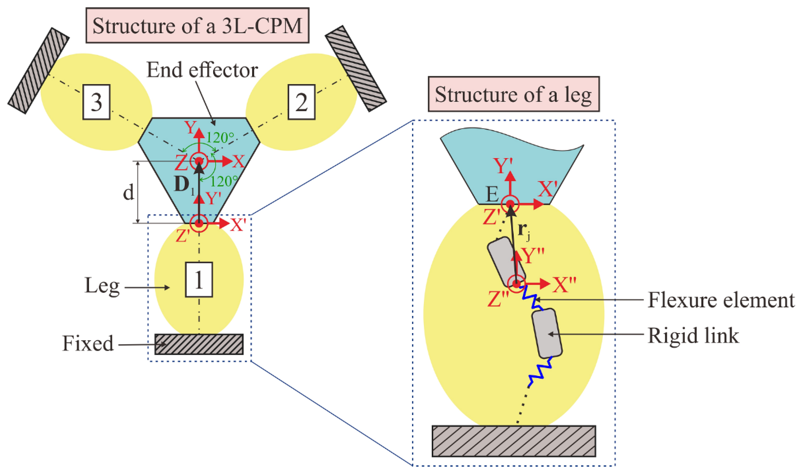
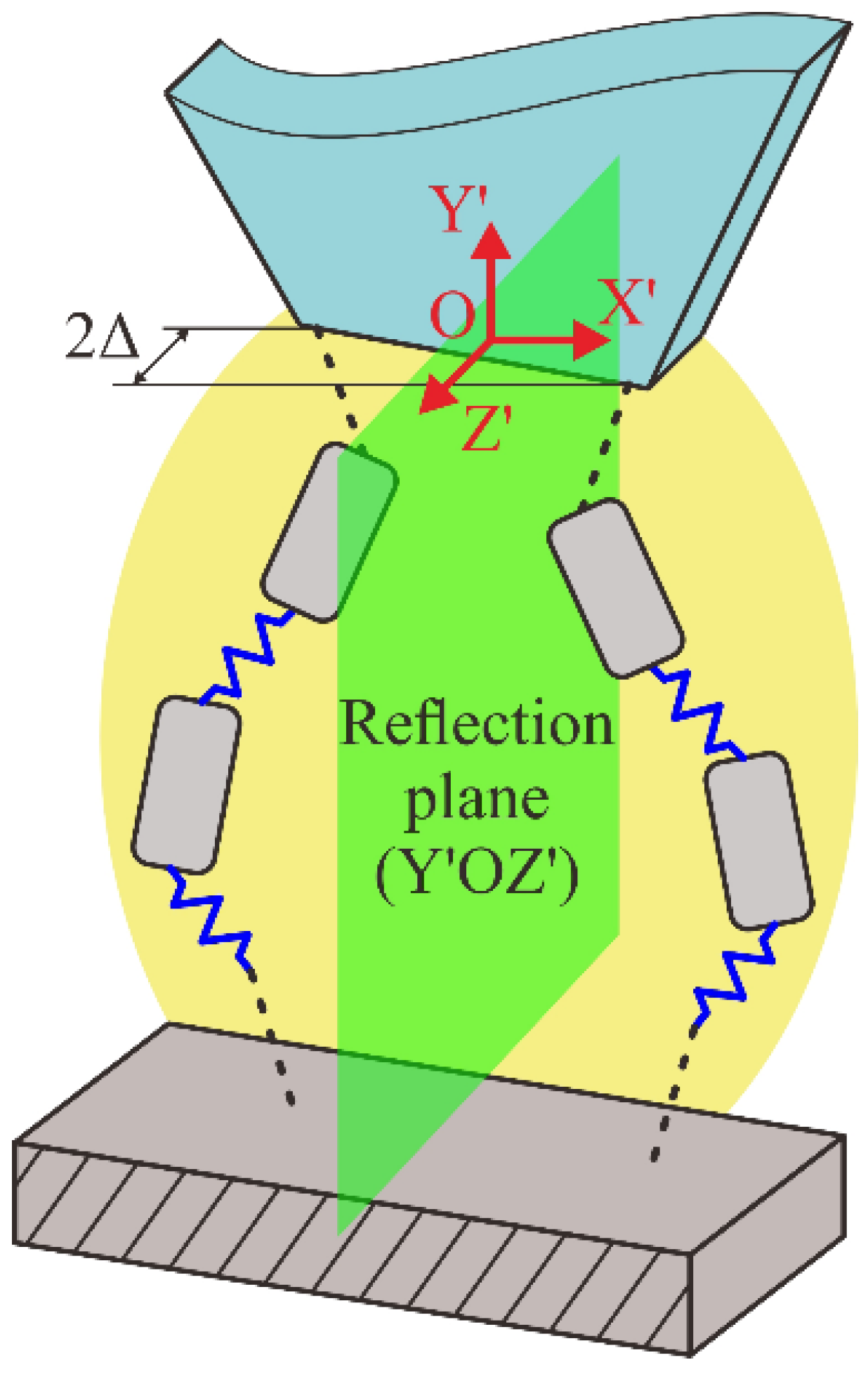
2. Stiffness Modeling of a Decoupled-Motion 3L-CPM

In this work, a CPM is represented by a mechanism having three compliant legs that are distributed symmetrically about the center of the end effector. The legs are fixed at one end, while the free ends are connected with the end effector. Each legs contains a serial chain of flexure elements and rigid links, as illustrated in Figure 1. Here, the global frame, XYZ, is attached to the center of the end effector, and the local frame of each leg, X′Y′Z′, is attached at the free end of each leg. Note that the X′Y′ plane of the local frame of each leg lies on the same plane as the XY plane of the global frame.

The stiffness property of a 3L-CPM is governed by the stiffness of the legs and the moving stage (end-effector). The stiffness matrix of the leg along the Y axis is represented by $K^l$ with respect to (w.r.t.) the local frame, i.e., at point E, as shown in Figure 1. With $D$ as the vector that represents the distance between the local frame of the leg and the global frame of the 3L-CPM, the stiffness matrix of the entire 3L-CPM, $K^m$, is expressed as follows:

$$K^m={\displaystyle \sum _{i=1}^3{J}_i^l{R}_i^l{K}^l{\left(R_i^l\right)}^{-1}{\left(J_i^l\right)}^T}$$

(1)

where i = 1, 2, and 3 denotes the three legs in the CPM, as illustrated in Figure 1; $J_i^l$ is the translation matrix from the local frame of the ith leg to the global frame; and $R_i^l$ is the rotation matrix about the Z axis of the ith leg. As three legs are symmetrical and 120° apart, $R_i^l$ and $J_i^l$ are written as follows:

$$R_i^l=\left[\begin{array}{cc}{R}_z\left({\theta }_i\right)& 0\\ 0& R_z\left({\theta }_i\right)\end{array}\right]\mathrm{where}{R}_z\left({\theta }_i\right)=\left[\begin{array}{ccc}\cos {\theta }_i& -\sin {\theta }_i& 0\\ \sin {\theta }_i& \cos {\theta }_i& 0\\ 0& 0& 1\end{array}\right]$$

(2)

$$J_i^l=\left[\begin{array}{cc}I& 0\\ T_i^l& I\end{array}\right]\mathrm{where}{T}_i^l=\left[\begin{array}{ccc}0& D_{z_i}& -D_{y_i}\\ -D_{z_i}& 0& D_{x_i}\\ D_{y_i}& -D_{x_i}& 0\end{array}\right]$$

(3)

In Equation (2), the values of ${\theta }_1$, ${\theta }_2$, and ${\theta }_3$ are 0°, 120°, and 240°, respectively. In Equation (3),$D_{x_i}$, $D_{y_i}$, and $D_{z_i}$ are three components of $D_i$ and represent the projections of the distance from each local frame to the global frame onto the X, Y, and Z axes, respectively. Note that $D_{z_i}=0$, since the X′Y′ plane of the local frames lies on the same plane as the XY plane of the global frame.

Here, the stiffness of a general leg, $K^l$, is represented as follows:

$$K^l=\left[\begin{array}{cccccc}{k}_{11}^l& & & & & \\ k_{21}^l& k_{22}^l& & & \mathrm{SYM}& \\ k_{31}^l& k_{32}^l& k_{33}^l& & & \\ k_{41}^l& k_{42}^l& k_{43}^l& k_{44}^l& & \\ k_{51}^l& k_{52}^l& k_{53}^l& k_{54}^l& k_{55}^l& \\ k_{61}^l& k_{62}^l& k_{63}^l& k_{64}^l& k_{65}^l& k_{66}^l\end{array}\right]$$

(4)

where the non-diagonal components are symmetrical. By substituting Equations (2)–(4) into Equation (1), the general form of the stiffness matrix of a 3L-CPM is as follows:

$$K^m=\left[\begin{array}{cccccc}{k}_{11}^m& & & & & \\ 0& k_{22}^m& & & \mathrm{SYM}& \\ 0& 0& k_{33}^m& & & \\ k_{41}^m& k_{42}^m& 0& k_{44}^m& & \\ k_{51}^m& k_{52}^m& 0& 0& k_{55}^m& \\ 0& 0& k_{63}^m& 0& 0& k_{66}^m\end{array}\right]$$

(5)

with d denoting the size of the end effector, as illustrated in Figure 1, the expressions of the non-zero components within the stiffness matrix of Equation (5) are expressed as follows:

$$\begin{array}{ll}{k}_{11}^m=& k_{22}^m=\frac{3}{2}\left(k_{11}^l+k_{22}^l\right)\\ k_{33}^m=& 3k_{33}^l\\ k_{44}^m=& k_{55}^m=\frac{3}{2}\left(d^2{k}_{33}^l-2d{k}_{43}^l+k_{44}^l+k_{55}^l\right)\\ k_{66}^m=& 3\left(d^2{k}_{11}^l+2d{k}_{61}^l+k_{66}^l\right)\\ k_{41}^m=& k_{52}^m=-\frac{3}{2}\left(d{k}_{31}^l-k_{41}^l-k_{52}^l\right)\\ k_{51}^m=& -k_{42}^m=\frac{3}{2}\left(k_{51}^l+d{k}_{32}^l-k_{42}^l\right)\\ k_{63}^m=& 3\left(d{k}_{31}^l+k_{63}^l\right)\end{array}$$

(6)

By referring to Equation (6), the five non-diagonal components within $K^m$ ($k_{41}^m$, $k_{42}^m$, $k_{51}^m$, $k_{52}^m$, and $k_{63}^m$) are represented by seven components within $K^l$ ($k_{31}^l$, $k_{32}^l$, $k_{41}^l$, $k_{42}^l$, $k_{51}^l$, $k_{52}^l$, and $k_{63}^l$). To fulfill the requirements of a fully decoupled motion, all non-diagonal components in $K^m$ must be zeros. In this work, the 6 × 6 stiffness matrix of a 3L-CPM with fully decoupled motion characteristic is termed as a diagonal stiffness matrix, as shown in Equation (7).

$$K^m=\left[\begin{array}{cccccc}{k}_{11}^m& & & & & \\ 0& k_{22}^m& & & \mathrm{SYM}& \\ 0& 0& k_{33}^m& & & \\ 0& 0& 0& k_{44}^m& & \\ 0& 0& 0& 0& k_{55}^m& \\ 0& 0& 0& 0& 0& k_{66}^m\end{array}\right]$$

(7)

In order to obtain a diagonal stiffness matrix as shown in Equation (7), the five non-diagonal components in Equation (5), for which the expressions are written in Equation (6), must be zeros. With $k_{41}^m=k_{52}^m$ and $k_{51}^m=-k_{42}^m$, the relationship between seven variables ($k_{31}^l$, $k_{32}^l$, $k_{41}^l$, $k_{42}^l$, $k_{51}^l$, $k_{52}^l$, and $k_{63}^l$) in $k_{41}^m$, $k_{42}^m$, $k_{51}^m$, $k_{52}^m$, and $k_{63}^m$ can only be represented by three equations, and this condition led to a multiple-solutions problem. Hence, it is important to note that this work only uses a special case (or solution) to demonstrate how the presented mathematical models can be used to synthesize a 3L-CPM with the aim of achieving fully decoupled motion capability. This special case is to make those seven components within $K^l$ be zeros, as shown in Equation (8).

$$K^l=\left[\begin{array}{cccccc}{k}_{11}^l& & & & & \\ k_{21}^l& k_{22}^l& & & \mathrm{SYM}& \\ 0& 0& k_{33}^l& & & \\ 0& 0& k_{43}^l& k_{44}^l& & \\ 0& 0& k_{53}^l& k_{54}^l& k_{55}^l& \\ k_{61}^l& k_{62}^l& 0& k_{64}^l& k_{65}^l& k_{66}^l\end{array}\right]$$

(8)

In this work, the two popular-choice flexure elements that are used to synthesize the compliant mechanisms are the beam type and the notch type, as shown in Figure 2. Both elements have thin features which permit elastic bending in a specific direction.

Assuming that each leg being formed by a serial chain of flexure elements and rigid links where a rigid link has infinite stiffness (non-compliance) property, the compliance of each leg ($C^l$) is governed by the compliance of each flexure element, $C_j^e$, expressed as follows:

$$C^l={\displaystyle \sum _{j=1}^n{J}_j^e{R}_j^e{C}_j^e{\left(R_j^e\right)}^{-1}{\left(J_j^e\right)}^T}$$

(9)

where n denotes the number of flexure elements, and $R_j^e$ and $J_j^e$ are the rotation matrix, and translation matrix of the jth flexure element respectively. Referring to Reference [57], the compliance matrix of each original flexure element, $C_j^e$, with respect to the local frame, as illustrated in Figure 2, is defined as follows:

$$C_j^e=\left[\begin{array}{cccccc}{c}_{11}^e& & & & & \\ 0& c_{22}^e& & & \mathrm{SYM}& \\ 0& 0& c_{33}^e& & & \\ 0& 0& 0& c_{44}^e& & \\ 0& 0& c_{53}^e& 0& c_{55}^e& \\ 0& c_{62}^e& 0& 0& 0& c_{66}^e\end{array}\right]$$

(10)

Equation (10) is applicable for both the beam type and notch type flexure elements, as illustrated in Figure 2 [57]. In addition, the geometry of each flexure element type can vary without changing the form of the compliant matrix expressed in Equation (10). Several kinds of flexure elements which have a similar form of compliance matrix are presented in Appendix A. Note that the X″Y″ plane of the local frame of each flexure element (Figure 2) lies on the parallel plane with the XY plane of the global frame, as illustrated in Figure 1. By referring to Equation (9), we see that the rotation matrix, $R_j^e$, is a 6 × 6 matrix and is defined as the multiplication of the rotation matrices about the X″, Y″, and Z″ axes ($R_{x_j}^e$, $R_{y_j}^e$ and $R_{z_j}^e$). Hence, it is written as follows:

$$\begin{array}{cc}{R}_j^e=\left[\begin{array}{cc}{R}_{z_j}^e{R}_{y_j}^e{R}_{x_j}^e& 0\\ 0& R_{z_j}^e{R}_{y_j}^e{R}_{x_j}^e\end{array}\right]\mathrm{where}& R_{z_j}^e=\left[\begin{array}{ccc}\cos {\gamma }_j& -\sin {\gamma }_j& 0\\ \sin {\gamma }_j& \cos {\gamma }_j& 0\\ 0& 0& 1\end{array}\right],\\ & R_{y_j}^e=\left[\begin{array}{ccc}\cos {\beta }_j& 0& \sin {\beta }_j\\ 0& 1& 0\\ -\sin {\beta }_j& 0& \cos {\beta }_j\end{array}\right],\\ & R_{x_j}^e=\left[\begin{array}{ccc}1& 0& 0\\ 0& \cos {\alpha }_j& -\sin {\alpha }_j\\ 0& \sin {\alpha }_j& \cos {\alpha }_j\end{array}\right]\end{array}$$

(11)

Here, ${\alpha }_j$, ${\beta }_j$, and ${\gamma }_j$ represent the rotation angles about the X″, Y″, and Z″ axes, respectively. The geometries of a flexure element before and after orientation are also illustrated in Figure 2. As for the 6 × 6 translation matrix, $J_j^e$, it represents the projected distances onto the three axes ($r_{x_j}$, $r_{y_j}$, and $r_{z_j}$) from the jth flexure element to the local frame of the leg that are indicated by vector $r_j$, as shown in Figure 1, written as follows:

$$J_j^e=\left[\begin{array}{cc}I& r_j^e\\ 0& I\end{array}\right]\mathrm{where}{r}_j^e=\left[\begin{array}{ccc}0& r_{z_j}& -r_{y_j}\\ -r_{z_j}& 0& r_{x_j}\\ r_{y_j}& -r_{x_j}& 0\end{array}\right]$$

(12)

Using Equations (9)–(12), the compliance matrix of a leg, $C^l$, can be obtained, and the stiffness matrix of each leg is given as $K^l={\left(C^l\right)}^{-1}$.

As mentioned earlier, the stiffness matrix of each leg must follow the exact form shown in Equation (8), and this requirement applies to its corresponding compliance matrix too. The detailed derivation of the compliance matrix of each leg with the aim of achieving that requirement is presented in Appendix B. To summarize the results obtained from Appendix B, one condition which allows for the compliance matrix of a leg to become the exact same form as Equation (8) is for seven components within the compliance matrix of a leg to be zeros, i.e., $c_{31}^l=c_{32}^l=c_{41}^l=c_{42}^l=c_{51}^l=c_{52}^l=c_{63}^l=0$. This condition offers simplicity during the design stage and can be used as the standard approach to synthesize 3L-CPMs with the aim of achieving fully decoupled motion capability. However, it also introduces a multiple-solutions problem to solve the corresponding components within the stiffness matrix, $K^l$. Among a number of possible solutions, $k_{64}^l=k_{65}^l=0$ is a unique solution that is used to fulfill the condition in this work. By adopting this unique solution, both the stiffness matrix and the compliance matrix of a leg will have the same form as expressed in Equation (13), and the expression of each component within $K^l$ is given in Appendix C.

$$\underset{K^l}{\underbrace{\left[\begin{array}{cccccc}{k}_{11}^l& & & & & \\ k_{21}^l& k_{22}^l& & & \mathrm{SYM}& \\ 0& 0& k_{33}^l& & & \\ 0& 0& k_{43}^l& k_{44}^l& & \\ 0& 0& k_{53}^l& k_{54}^l& k_{55}^l& \\ k_{61}^l& k_{62}^l& 0& 0& 0& k_{66}^l\end{array}\right]}}=\underset{{\left(C^l\right)}^{-1}}{\underbrace{{\left[\begin{array}{cccccc}{c}_{11}^l& & & & & \\ c_{21}^l& c_{22}^l& & & \mathrm{SYM}& \\ 0& 0& c_{33}^l& & & \\ 0& 0& c_{43}^l& c_{44}^l& & \\ 0& 0& c_{53}^l& c_{54}^l& c_{55}^l& \\ c_{61}^l& c_{62}^l& 0& 0& 0& c_{66}^l\end{array}\right]}^{-1}}}$$

(13)

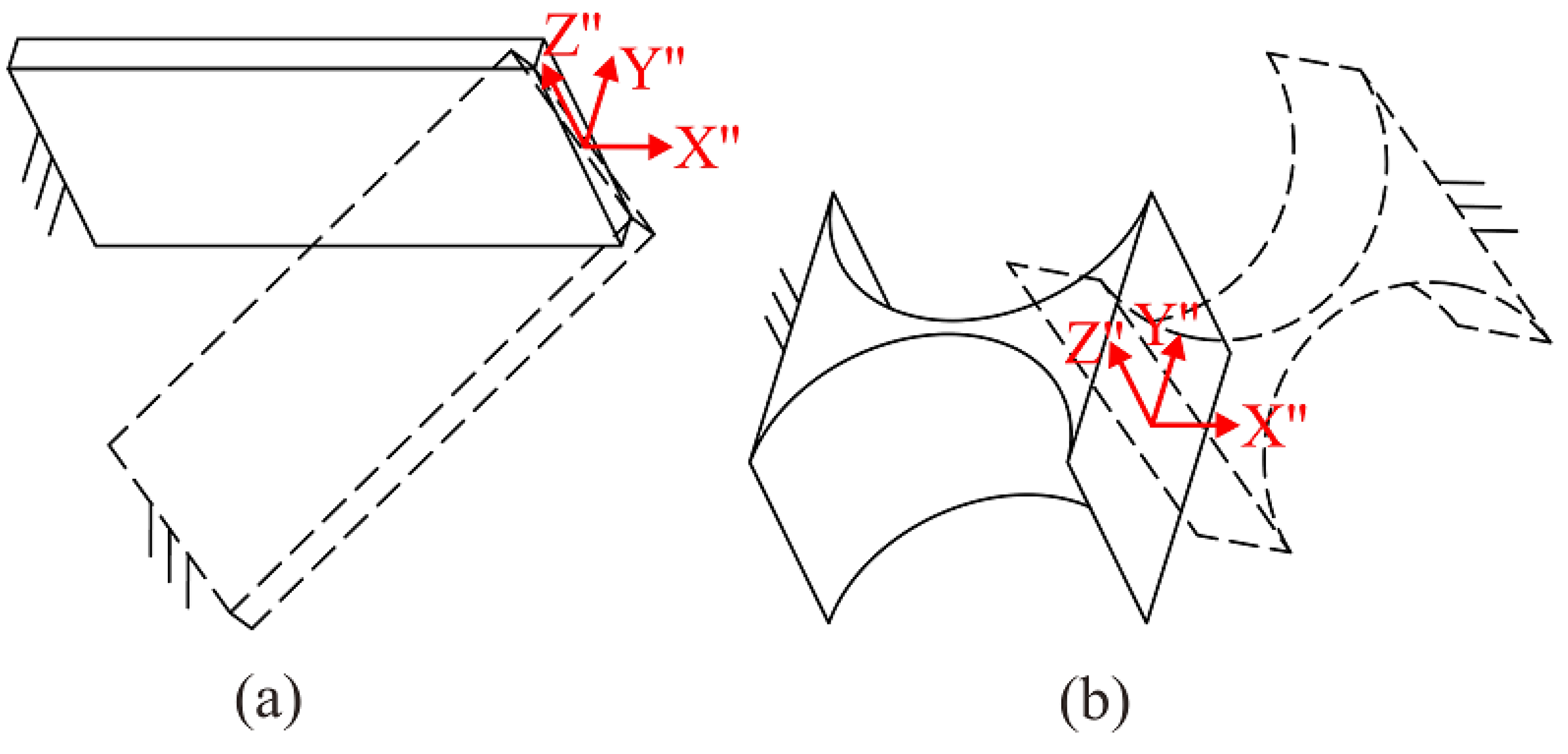
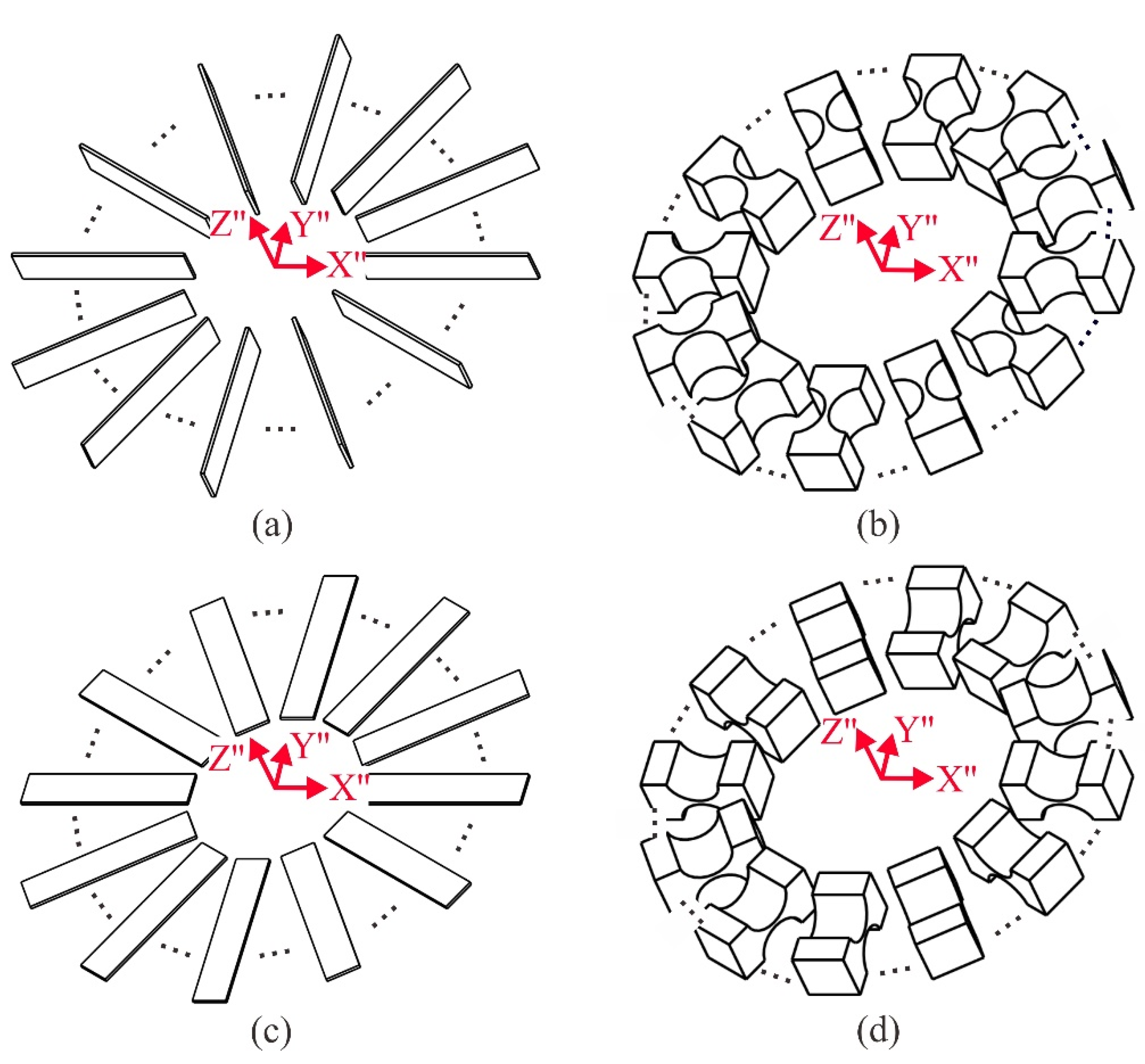
3. Characteristics of Flexure Elements in Decoupled-Motion 3L-CPMs

In this section, the desired rotation angles ($\alpha$, $\beta$, and $\gamma$) and distances ($r_x$, $r_y$, and $r_z$) of flexure elements in a leg to achieve decoupled-motion capability are analyzed. First, Equation (9) is re-expressed as follows:

$$K^l={\left(C^l\right)}^{-1}={\left({\displaystyle \sum _{j=1}^n{J}_j^e{R}_j^e{C}_j^e{\left(R_j^e\right)}^{-1}{\left(J_j^e\right)}^T}\right)}^{-1}={\left({\displaystyle \sum _{j=1}^n{\overline{C}}_j^e}\right)}^{-1}$$

(14)

where ${\overline{C}}_j^e$ indicates the compliance matrix of the jth oriented flexure element referring to the local frame X′Y′Z′ attached to the free end of the leg, as illustrated in Figure 1. In order to achieve fully decoupled motion, the nine non-diagonal components ($c_{31}^l$, $c_{41}^l$, $c_{51}^l$, $c_{32}^l$, $c_{42}^l$, $c_{52}^l$, $c_{63}^l$, $c_{64}^l$, and $c_{65}^l$) of the compliance matrix, $C^l$, must be zeros, as shown in Equation (13). As $C^l$ is the sum of n sub-components, ${\overline{C}}_j^e$, there could be numerous solutions, because all components within ${\overline{C}}_j^e$ can have arbitrary values in general cases. In this work, a special case where all ${\overline{C}}_j^e$ have the same form (${\overline{C}}^e$) is considered and yields the following:

$${\overline{C}}^e=\left[\begin{array}{llllll}{\overline{c}}_{11}^e\hfill & \hfill & \hfill & \hfill & \hfill & \hfill \\ {\overline{c}}_{21}^e\hfill & {\overline{c}}_{22}^e\hfill & \hfill & \hfill & \mathrm{SYM}\hfill & \hfill \\ {\overline{c}}_{31}^e=0\hfill & {\overline{c}}_{32}^e=0\hfill & {\overline{c}}_{33}^e\hfill & \hfill & \hfill & \hfill \\ {\overline{c}}_{41}^e=0\hfill & {\overline{c}}_{42}^e=0\hfill & {\overline{c}}_{43}^e\hfill & {\overline{c}}_{44}^e\hfill & \hfill & \hfill \\ {\overline{c}}_{51}^e=0\hfill & {\overline{c}}_{52}^e=0\hfill & {\overline{c}}_{53}^e\hfill & {\overline{c}}_{54}^e\hfill & {\overline{c}}_{55}^e\hfill & \hfill \\ {\overline{c}}_{61}^e\hfill & {\overline{c}}_{62}^e\hfill & {\overline{c}}_{63}^e=0\hfill & {\overline{c}}_{64}^e=0\hfill & {\overline{c}}_{65}^e=0\hfill & {\overline{c}}_{66}^e\hfill \end{array}\right]$$

(15)

Note that ${\overline{C}}^e$ in Equation (15) is different from $C^e$ in Equation (10), since ${\overline{C}}^e=J^e{R}^e{C}^e{\left(R^e\right)}^{-1}{\left(J^e\right)}^T$, as expressed in Equation (14). $R^e$ and $J^e$ are similar to Equations (11) and (12) with the subscript, j, being removed.

Equation (15) describes the condition to obtain a 3L-CPM with fully decoupled motion capability, expressed by nine equations that can be obtained based on those nine zero components. There are six unknowns in these equations, i.e., the rotation angles ($\alpha$, $\beta$, and $\gamma$) and the distances ($r_x$, $r_y$, and $r_z$) measured from the moving end of the flexure element to the free end of the leg.

$$\begin{array}{ll}{\overline{c}}_{31}^e& =-c_{11}^e\sin \beta \cos \beta \cos \gamma +c_{44}^e\cos \beta \left(r_y\cos \gamma -r_x\sin \gamma \right)\left(r_y\sin \beta +r_z\cos \beta \sin \gamma \right)-\\ & \cos \beta \sin \alpha \left\{\cos \gamma \sin \alpha \left(c_{62}^e{r}_z-c_{22}^e\sin \beta \right)+\cos \alpha \left[c_{62}^e{r}_y\cos \beta +\left(c_{22}^e-c_{62}^e{r}_z\sin \beta \right)\sin \gamma \right]\right\}+\\ & \cos \alpha \cos \beta \left\{\cos \alpha \cos \gamma \left(c_{53}^e{r}_z+c_{33}^e\sin \beta \right)+\sin \alpha \left[-c_{53}^e{r}_y\cos \beta +\left(c_{33}^e+c_{53}^e{r}_z\sin \beta \right)\sin \gamma \right]\right\}+\\ & \left[\sin \alpha \sin \beta \left(r_y\cos \gamma -r_x\sin \gamma \right)-\cos \alpha \left(r_x\cos \gamma +r_y\sin \gamma \right)\right]\cdot \\ & \left\{\cos \alpha \cos \gamma \left(c_{55}^e{r}_z+c_{53}^e\sin \beta \right)+\sin \alpha \left[-c_{55}^e{r}_y\cos \beta +\left(c_{53}^e+c_{55}^e{r}_z\sin \beta \right)\sin \gamma \right]\right\}+\\ & \left[\cos \gamma \left(r_x\sin \alpha +r_y\cos \alpha \sin \beta \right)+\left(r_y\sin \alpha -r_x\cos \alpha \sin \beta \right)\sin \gamma \right]\cdot \\ & \left\{\cos \gamma \sin \alpha \left(-c_{66}^e{r}_z+c_{62}^e\sin \beta \right)-\cos \alpha \left[c_{66}^e{r}_y\cos \beta +\left(c_{62}^e-c_{66}^e{r}_z\sin \beta \right)\sin \gamma \right]\right\}\end{array}$$

(16)

$$\begin{array}{ll}{\overline{c}}_{41}^e& =c_{44}^e\cos \beta \cos \gamma \left(r_y\sin \beta +r_z\cos \beta \sin \gamma \right)+\left(\cos \gamma \sin \alpha \sin \beta -\cos \alpha \sin \gamma \right)\cdot \\ & \left\{\cos \alpha \cos \gamma \left(c_{55}^e{r}_z+c_{53}^e\sin \beta \right)+\sin \alpha \left[-c_{55}^e{r}_y\cos \beta +\left(c_{53}^e+c_{55}^e{r}_z\sin \beta \right)\sin \gamma \right]\right\}+\\ & \left(\cos \alpha \cos \gamma \sin \beta +\sin \alpha \sin \gamma \right)\cdot \\ & \left\{\cos \gamma \sin \alpha \left(-c_{66}^e{r}_z+c_{62}^e\sin \beta \right)-\cos \alpha \left[c_{66}^e{r}_y\cos \beta +\left(c_{62}^e-c_{66}^e{r}_z\sin \beta \right)\sin \gamma \right]\right\}\end{array}$$

(17)

$$\begin{array}{ll}{\overline{c}}_{51}^e& =c_{44}^e\cos \beta \sin \gamma \left(r_y\sin \beta +r_z\cos \beta \sin \gamma \right)+\left(\cos \alpha \cos \gamma +\sin \alpha \sin \beta \sin \gamma \right)\cdot \\ & \left\{\cos \alpha \cos \gamma \left(c_{55}^e{r}_z+c_{53}^e\sin \beta \right)+\sin \alpha \left[-c_{55}^e{r}_y\cos \beta +\left(c_{53}^e+c_{55}^e{r}_z\sin \beta \right)\sin \gamma \right]\right\}+\\ & \left(-\cos \gamma \sin \alpha +\cos \alpha \sin \beta \sin \gamma \right)\cdot \\ & \left\{\cos \gamma \sin \alpha \left(-c_{66}^e{r}_z+c_{62}^e\sin \beta \right)-\cos \alpha \left[c_{66}^e{r}_y\cos \beta +\left(c_{62}^e-c_{66}^e{r}_z\sin \beta \right)\sin \gamma \right]\right\}\end{array}$$

(18)

$$\begin{array}{ll}{\overline{c}}_{32}^e& =-c_{11}^e\cos \beta \sin \beta \sin \gamma -c_{44}^e\cos \beta \left(r_z\cos \beta \cos \gamma +r_x\sin \beta \right)\left(r_y\cos \gamma -r_x\sin \gamma \right)+\\ & \cos \beta \sin \alpha \left\{\cos \alpha \left[c_{62}^e{r}_x\cos \beta +\cos \gamma \left(c_{22}^e-c_{62}^e{r}_z\sin \beta \right)\right]+\sin \alpha \left(-c_{62}^e{r}_z+c_{22}^e\sin \beta \right)\sin \gamma \right\}+\\ & \cos \alpha \cos \beta \left[c_{53}^e{r}_x\cos \beta \sin \alpha -\cos \gamma \sin \alpha \left(c_{33}^e+c_{53}^e{r}_z\sin \beta \right)+\cos \alpha \left(c_{53}^e{r}_z+c_{33}^e\sin \beta \right)\sin \gamma \right]+\\ & \left\{\cos \alpha \left[c_{66}^e{r}_x\cos \beta +\cos \gamma \left(c_{62}^e-c_{66}^e{r}_z\sin \beta \right)\right]+\sin \alpha \left(-c_{66}^e{r}_z+c_{62}^e\sin \beta \right)\sin \gamma \right\}\cdot \\ & \left[\cos \gamma \left(r_x\sin \alpha +r_y\cos \alpha \sin \beta \right)+\left(r_y\sin \alpha -r_x\cos \alpha \sin \beta \right)\sin \gamma \right]+\\ & \left[c_{55}^e{r}_x\cos \beta \sin \alpha -\cos \gamma \sin \alpha \left(c_{53}^e+c_{55}^e{r}_z\sin \beta \right)+\cos \alpha \left(c_{55}^e{r}_z+c_{53}^e\sin \beta \right)\sin \gamma \right]\cdot \\ & \left[\sin \alpha \sin \beta \left(r_y\cos \gamma -r_x\sin \gamma \right)-\cos \alpha \left(r_x\cos \gamma +r_y\sin \gamma \right)\right]\end{array}$$

(19)

$$\begin{array}{ll}{\overline{c}}_{42}^e& =-c_{44}^e\cos \beta \cos \gamma \left(r_z\cos \beta \cos \gamma +r_x\sin \beta \right)+\left(\cos \alpha \cos \gamma \sin \beta +\sin \alpha \sin \gamma \right)\cdot \\ & \left\{\cos \alpha \left[c_{66}^e{r}_x\cos \beta +\cos \gamma \left(c_{62}^e-c_{66}^e{r}_z\sin \beta \right)\right]+\sin \alpha \left(-c_{66}^e{r}_z+c_{62}^e\sin \beta \right)\sin \gamma \right\}+\\ & \left(\cos \gamma \sin \alpha \sin \beta -\cos \alpha \sin \gamma \right)\cdot \\ & \left[c_{55}^e{r}_x\cos \beta \sin \alpha -\cos \gamma \sin \alpha \left(c_{53}^e+c_{55}^e{r}_z\sin \beta \right)+\cos \alpha \left(c_{55}^e{r}_z+c_{53}^e\sin \beta \right)\sin \gamma \right]\end{array}$$

(20)

$$\begin{array}{ll}{\overline{c}}_{52}^e& =-c_{44}^e\cos \beta \left(r_z\cos \beta \cos \gamma +r_x\sin \beta \right)\sin \gamma +\left(-\cos \gamma \sin \alpha +\cos \alpha \sin \beta \sin \gamma \right)\cdot \\ & \left\{\cos \alpha \left[c_{66}^e{r}_x\cos \beta +\cos \gamma \left(c_{62}^e-c_{66}^e{r}_z\sin \beta \right)\right]+\sin \alpha \left(-c_{66}^e{r}_z+c_{62}^e\sin \beta \right)\sin \gamma \right\}+\\ & \left(\cos \alpha \cos \gamma +\sin \alpha \sin \beta \sin \gamma \right)\cdot \\ & \left[c_{55}^e{r}_x\cos \beta \sin \alpha -\cos \gamma \sin \alpha \left(c_{53}^e+c_{55}^e{r}_z\sin \beta \right)+\cos \alpha \left(c_{55}^e{r}_z+c_{53}^e\sin \beta \right)\sin \gamma \right]\end{array}$$

(21)

$$\begin{array}{ll}{\overline{c}}_{63}^e& =\frac{1}{2}\cos \beta \{\left(c_{62}^e+c_{53}^e\right)\cos \beta \sin 2\alpha +\left[2c_{44}^e-c_{55}^e-c_{66}^e+\left(c_{55}^e-c_{66}^e\right)\cos 2\alpha \right]\cdot \\ & \sin \beta \left(-r_y\cos \gamma +r_x\sin \gamma \right)-\left(c_{55}^e-c_{66}^e\right)\sin 2\alpha \left(r_x\cos \gamma +r_y\sin \gamma \right)\}\end{array}$$

(22)

$${\overline{c}}_{64}^e=\cos \beta \left[\cos \gamma \left(-c_{44}^e+c_{66}^e{\cos }^2\alpha +c_{55}^e{\sin }^2\alpha \right)\sin \beta +\left(-c_{55}^e+c_{66}^e\right)\cos \alpha \sin \alpha \sin \gamma \right]$$

(23)

$${\overline{c}}_{65}^e=\cos \beta \left[\left(c_{55}^e-c_{66}^e\right)\cos \alpha \cos \gamma \sin \alpha +c_{66}^e{\cos }^2\alpha \sin \beta \sin \gamma +\left(-c_{44}^e+c_{55}^e{\sin }^2\alpha \right)\sin \beta \sin \gamma \right]$$

(24)

This set of equations can be solved by considering Equation (22) first, because $\beta$ is the only dominant angular variable, and the results are given as follows:

$${\overline{c}}_{63}^e=0\iff [\begin{array}{l}\beta =90°\\ \alpha =0°\mathrm{and}\beta =0°,180°\\ \alpha =90°\mathrm{and}\beta =0°,180°\end{array};\forall \gamma ,r_x,r_y,r_z$$

(25)

Here, the rotation angle about the X″ axis, $\alpha$, varies from 0° to 90°, because of the symmetrical structure of the flexure elements, as illustrated in Figure 2. Equation (25) shows that there are three possible cases for, ${\overline{c}}_{63}^e=0$ with the four remaining variables ($\gamma$, $r_x$, $r_y$, and $r_z$) being arbitrary values.

First, the case with $\beta =90°$ is considered. With every component within the compliance matrix of the flexure element having a specific value, as shown in Equation (10), six Equations, from (16) to (21), are always different from zero with any value of $\gamma$, $r_x$, $r_y$, and $r_z$. Hence, $\beta =90°$ is not a feasible solution.

Next, consider the second case with $\alpha =0°$ and $\beta =0°,\hspace{0.17em}180°$; the following results can be obtained:

$$\begin{array}{l}{\overline{c}}_{31}^e=\pm r_z\left\{\mp c_{55}^e{r}_x{\cos }^2\gamma \mp c_{44}^e{r}_x{\sin }^2\gamma +\cos \gamma \left[c_{53}^e+\left(\pm c_{44}^e\mp c_{55}^e\right)r_y\sin \gamma \right]\right\}\\ {\overline{c}}_{41}^e=\left(c_{44}^e-c_{55}^e\right)r_z\cos \gamma \sin \gamma \\ {\overline{c}}_{51}^e=r_z\left(c_{55}^e{\cos }^2\gamma +c_{44}^e{\sin }^2\gamma \right)\\ {\overline{c}}_{32}^e=\pm r_z\left[\mp c_{44}^e{r}_y{\cos }^2\gamma +\left(\pm c_{44}^e\mp c_{55}^e\right)r_x\cos \gamma \sin \gamma +\sin \gamma \left(c_{53}^e\mp c_{55}^e{r}_y\sin \gamma \right)\right]\\ {\overline{c}}_{42}^e=-r_z\left(c_{44}^e{\cos }^2\gamma +c_{55}^e{\sin }^2\gamma \right)\\ {\overline{c}}_{52}^e=\left(-c_{44}^e+c_{55}^e\right)r_z\cos \gamma \sin \gamma \\ {\overline{c}}_{64}^e={\overline{c}}_{65}^e=0\end{array}$$

(26)

Here, the upper signs of “$\pm$” and “$\mp$” in Equation (26) represent the case of $\alpha =0°$ and $\beta =0°$, while the lower signs represent the case of $\alpha =0°$ and $\beta =180°$. To solve Equation (26), ${\overline{c}}_{51}^e$ is first considered to be equal to zero, a unique solution can be obtained $r_z=0$ by, and $\gamma$ can be any value. With $r_z=0$, all the remaining equations in Equation (26) will also be equal to zeros. Hence, $r_z=0$, $\alpha =0°$, $\beta =0°\hspace{0.17em}\mathrm{or}\hspace{0.17em}180°$ are solutions used to obtain a 3L-CPM with any DOF and decoupled motions.

Similarly, for the case with $\alpha =90°$ and $\beta =0°\mathrm{or}180°$, it can be shown that this is also a possible solution. In summary, the two feasible solutions found from Equation (25) with $r_z=0$ are as follows:

$$[\begin{array}{l}\alpha =0°\mathrm{and}\beta =0°,180°\hfill \\ \alpha =90°\mathrm{and}\beta =0°,180°\hfill \end{array};\forall \gamma ,r_x,r_y$$

(27)

Equation (27) provides the design criteria for the orientations and positions of the flexure elements that need to be satisfied to design a 3L-CPM with fully decoupled motion capability. Figure 3 illustrates the desired orientation of the flexure elements about the X″ and Y″ axes, with various orientations about the Z″ axis. With flexure elements in a leg having these orientations and distributing in the X′Y′ plane ($r_z=0$), a 3L-CPM is able to achieve fully decoupled motions.

4. Stiffness Analysis of 3L-CPMs Containing Two Serial Flexure Chains in a Leg

In Section 2, the stiffness modeling of a general 3L-CPM, with each leg consisting of a single serial flexure chain, is presented. However, there are many existing 3L-CPMs synthesized by constraint-based and optimization methods that have two reflecting (or symmetrical) serial flexure chains, as shown in Figure 4 [6,7,28,31,42,43,53,55,56,58]. In this section, the analysis of such a leg configuration is presented.

From the literature [6,7,28,31,42,43,53,55,56,58], we can see that the double flexure chains are either on the same plane or have an offset distance of 2∆ along the Z′ axis, as shown in Figure 4. The stiffness matrix of each leg is expressed as follows:

$$K^l={\left({\displaystyle \sum _{j=1}^n{J}_{\left(+\mathrm{\Delta }\right)}{C}^{sc}{J}_{\left(+\mathrm{\Delta }\right)}^T}\right)}^{-1}+{\left({\displaystyle \sum _{j=1}^n{J}_{\left(-\mathrm{\Delta }\right)}M{C}^{sc}{M}^T{J}_{\left(-\mathrm{\Delta }\right)}^T}\right)}^{-1}$$

(28)

where $M$ is the reflection matrix about the Y′Z′ plane given in Equation (29); and $J_{\left(+\mathrm{\Delta }\right)}$ and $J_{\left(-\mathrm{\Delta }\right)}$ represent the offset matrices used to shift the original flexure chain and the reflecting flexure chain along the Z′-axis distances of +∆ and −∆, respectively, as given in Equation (30).

$$M=\left[\begin{array}{cccccc}-1& 0& 0& 0& 0& 0\\ 0& 1& 0& 0& 0& 0\\ 0& 0& 1& 0& 0& 0\\ 0& 0& 0& -1& 0& 0\\ 0& 0& 0& 0& 1& 0\\ 0& 0& 0& 0& 0& 1\end{array}\right]$$

(29)

$$J_{\left(\pm \mathrm{\Delta }\right)}=\left[\begin{array}{cccccc}1& 0& 0& 0& 0& 0\\ 0& 1& 0& 0& 0& 0\\ 0& 0& 1& 0& 0& 0\\ 0& \pm \mathrm{\Delta }& 0& 1& 0& 0\\ \mp \mathrm{\Delta }& 0& 0& 0& 1& 0\\ 0& 0& 0& 0& 0& 1\end{array}\right]$$

(30)

Here, $C^{sc}$ is the compliance matrix of a serial flexure chain that can be calculated by Equation (9). The results from Section 3 are used to analyze the stiffness property of 3L-CPMs with two reflecting flexure chains. After substituting Equations (9), (14), (29) and (30) into Equation (28), the results show that the decoupled motion capability can only be achieved when the offset distance 2∆ = 0 (or ∆ = 0). The offset distance can be considered as the translation component along the Z axis of each flexure elements ($r_{z_j}$) that can lead coupled motions, as mentioned before. Most important, to achieve fully decoupled output motion, $C^{sc}$ must be in the following form:

$$C^{sc}=\left[\begin{array}{cccccc}{c}_{11}^{sc}& & & & & \\ c_{21}^{sc}& c_{22}^{sc}& & & \mathrm{SYM}& \\ 0& 0& c_{33}^{sc}& & & \\ 0& 0& c_{43}^{sc}& c_{44}^{sc}& & \\ 0& 0& c_{53}^{sc}& c_{54}^{sc}& c_{55}^{sc}& \\ c_{61}^{sc}& c_{62}^{sc}& 0& 0& 0& c_{66}^{sc}\end{array}\right]$$

(31)

5. Review and Analysis of the Motion Characteristics of Existing 3L-CPMs

In Section 2, Section 3 and Section 4, 3L-CPMs constructed with single or double serial flexure chains in a leg together with their corresponding stiffness modeling and decoupled design criteria were presented. In this section, the proposed criteria are used to analyze the decoupled-motion capability of some existing 3L-CPM designs. It can be seen that the analysis provides insight into the motion characteristics of 3L-CPMs. With the design criteria for synthesizing 3L-CPMs with fully decoupled motions being provided and the motion-decoupling capability of popular 3L-CPM designs being clearly defined, designers can select or synthesize any 3L-CPM with suitable motion property (coupled or decoupled) for their specific applications.

This section presents a short review on the motion characteristics from some of the existing 3L-CPMs. For each CPM, either the compliance matrix of a leg/serial flexure chain or the stiffness/compliance matrix of the entire mechanism was derived and used to determine the theoretical motion characteristics. For 3L-CPMs having a single serial flexure chain in each leg, fully decoupled motion can be achieved if the compliance matrix of the leg is in the form of Equation (13). The full stiffness matrix of the entire 3L-CPMs can then be calculated by using Equations (5), (6) and (14). For 3L-CPMs containing two reflecting serial flexure chains in each leg, fully decoupled motion can be obtained if the compliance matrix of a serial flexure chain is similar to Equation (31), and the full stiffness matrix of entire CPM can be calculated based on Equations (5), (6) and (28). Note that the analyses were conducted for general cases where most parameters, such as rotations angles and distances, are symbolic. Therefore, the obtained results are in general forms, while the results for some specific designs were obtained by substituting values into the parameters.

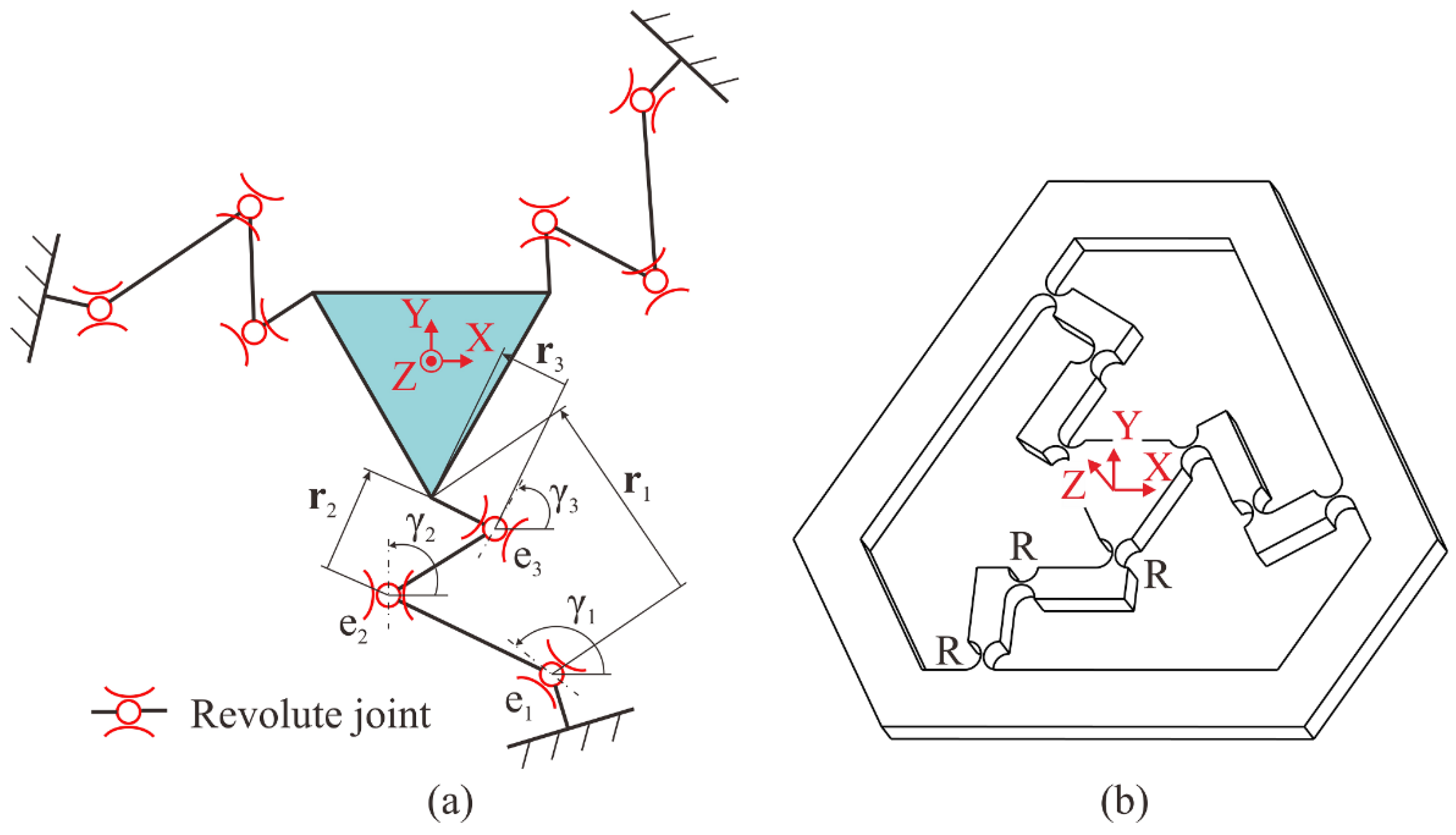
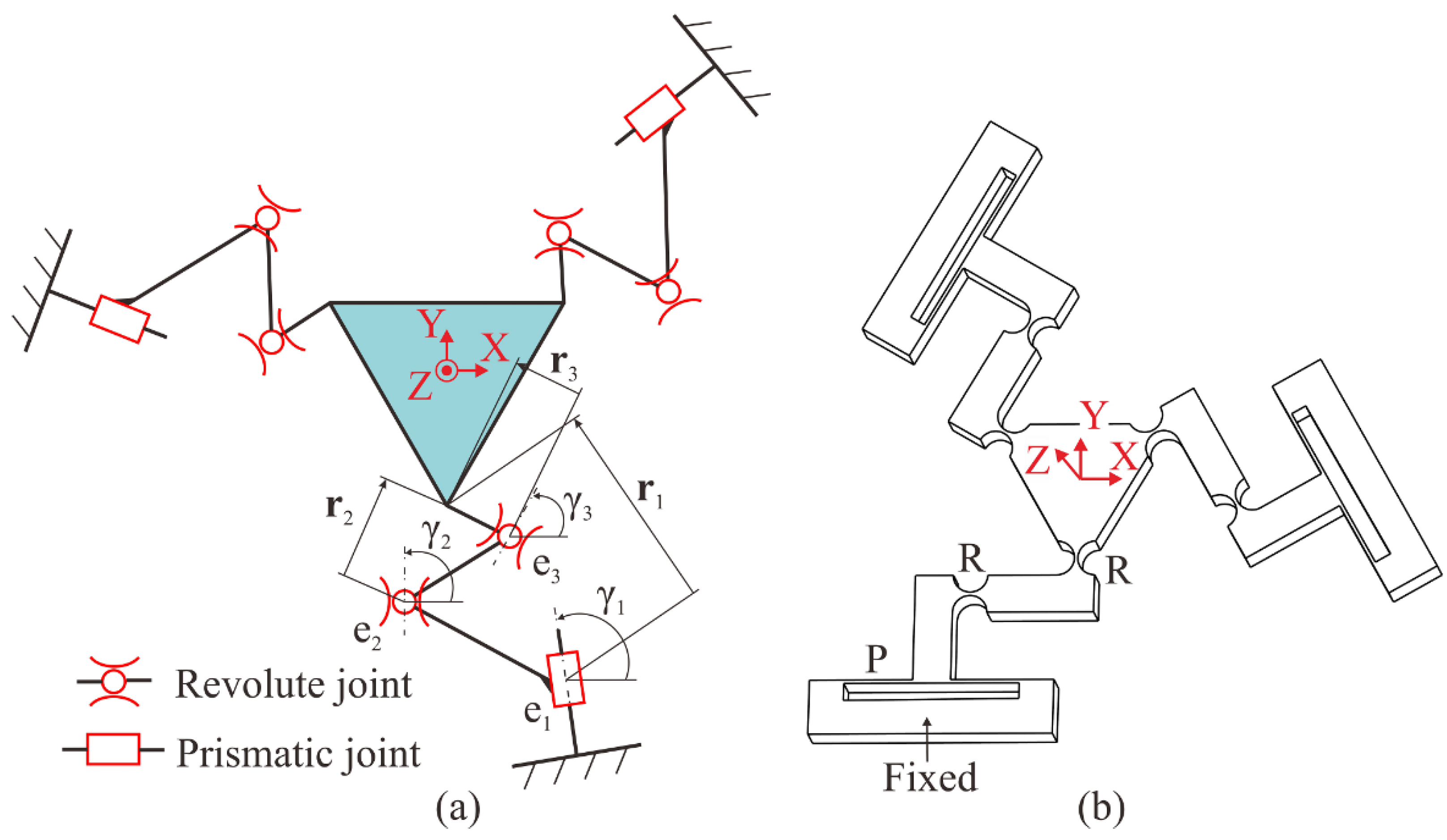
5.1. Three-Legged Revolute–Revolute–Revolute and Three-Legged Prismatic–Revolute–Revolute CPMs

The Three-legged Revolute–Revolute–Revolute (3RRR) configuration has been the most popular design for developing 3-DOF 3L-CPMs with (X-Y-θ_Z) planar motions, which are widely used in positioning/alignment systems [18,19,20,22,27,29,35,41]. The schematic diagram of a typical 3RRR-CPM is illustrated in Figure 5a, while Figure 6a illustrates the three-legged Prismatic–Revolute–Revolute (3PRR) configuration, which is a variant of 3RRR, where a revolute joint is replaced by a prismatic joint. The 3PRR-CPMs are preferred to create 3-DOF planar motions in MEMS devices, due to their advantage in actuation [59,60]. The prismatic joint can be designed as an active joint and easily driven by a linear actuator. Note that all flexure elements must be in the XY plane to create three desired motions. The physical prototypes of positioning systems developed based on 3RRR- and 3PRR-CPMs are shown in Figure 5b and Figure 6b, respectively.

To determine the theoretical motion characteristics of 3RRR-CPM or 3PRR-CPM, the compliance matrix of each flexure element is represented by $C_1^e$, $C_2^e$, and $C_3^e$, respectively, and each compliance matrix has a similar form to the one shown in Equation (10). Here, $C_1^e$ is the compliance matrix of either the first revolute joint within a 3RRR-CPM or the first prismatic joint within a 3PRR-CPM. $C_2^e$ and $C_3^e$ are the compliance matrices of the second and third revolute joints, respectively. As illustrated in Figure 5a and Figure 6a, each joint has a different orientation about the Z″ axis, ${\gamma }_j$, and a different distance to the moving end point, $r_j$, with j = 1, 2, and 3. The projections of $r_j$ onto the X and Y axes are $r_{x_j}$ and $r_{y_j}$, respectively. Based on Equation (9), the formula to calculate the compliance matrix of a leg is written as follows:

$$C^l={\displaystyle \sum _{j=1}^3{J}_j^e{R}_j^e{C}_j^e{\left(R_j^e\right)}^{-1}{\left(J_j^e\right)}^T}$$

(32)

where $J_j^e$ and $R_j^e$ are obtained by using Equations (12) and (11), respectively. The result of Equation (32) is shown in Equation (33), and the detailed expression of each component is given in Appendix D. It is observed that the compliance matrix of each leg within the 3RRR-CPMs and 3PRR-CPMs is similar to the form expressed in Equation (13). Hence, this observation suggests that the 3RRR and 3PRR configurations are able to deliver fully decoupled motion. This performance indicator also highlighted why both configurations are popular designs for developing state-of-the-art 3L-CPMs.

$$C^l=\left[\begin{array}{cccccc}{c}_{11}^l& & & & & \\ c_{21}^l& c_{22}^l& & & \mathrm{SYM}& \\ 0& 0& c_{33}^l& & & \\ 0& 0& c_{43}^l& c_{44}^l& & \\ 0& 0& c_{53}^l& c_{54}^l& c_{55}^l& \\ c_{61}^l& c_{62}^l& 0& 0& 0& c_{66}^l\end{array}\right]$$

(33)

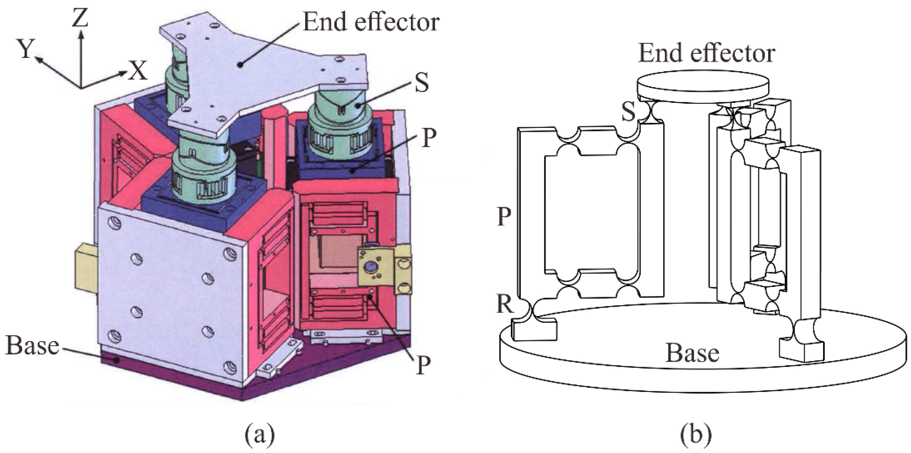
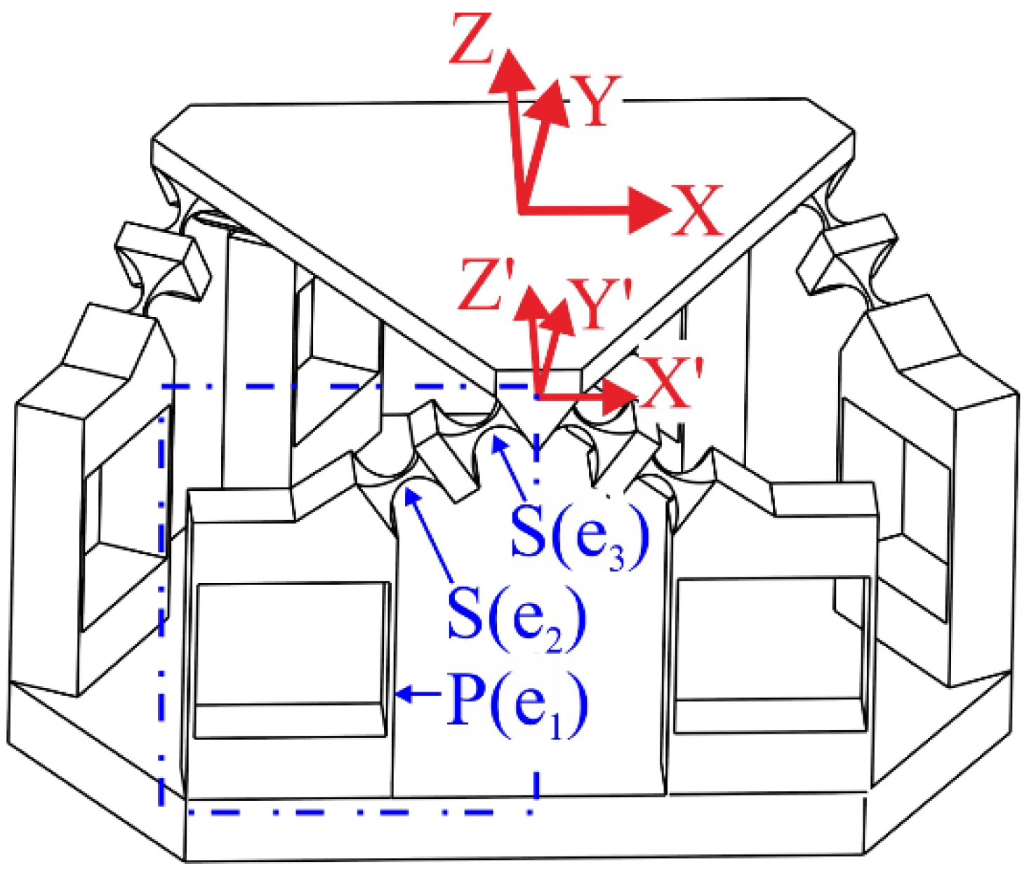
5.2. Three-Legged Prismatic–Prismatic–Spherical and Three-Legged Revolute–Prismatic–Spherical CPMs

Based on past works in the literature, the three-legged Prismatic–Prismatic–Spherical (3PPS) [5,32] and the three-legged Revolute–Prismatic–Spherical (3RPS) [21,61] configurations were adopted to develop 3-DOF 3L-CPMs with (θ_X-θ_Y-Z) out-of-plane motions, as shown in Figure 7a,b respectively. For both 3L-CPMs, each leg employed three serially connected flexure elements along the Z axis to create the desired motions. As a result, the component $r_{z_j}$ in Equation (12) exists and generates the off-axis components in the compliance matrix of a flexure element after transformation (${\overline{C}}_j^e$). Here, the components within $C^l$ can be derived from the following:

$$c_{ab}^l={\displaystyle \sum _{j=1}^3{\overline{c}}_{ab}^{e_j}}$$

(34)

where ${\overline{c}}_{ab}^{e_j}$ is a component on row a and column b in ${\overline{C}}_j^e$ calculated by Equation (14).

Based on the results obtained from Equation (16) to Equation (24), the components, i.e., ${\overline{c}}_{31}^{e_j}$, ${\overline{c}}_{41}^{e_j}$, ${\overline{c}}_{51}^{e_j}$, ${\overline{c}}_{32}^{e_j}$, ${\overline{c}}_{42}^{e_j}$, and ${\overline{c}}_{52}^{e_j}$, are non-zeros because of the existence of $r_{z_j}$. Thus, the corresponding components in $C^l$ are also non-zeros. Therefore, the legs’ compliance matrices within the 3PPS- and 3RPS-CPMs do not satisfy Equation (13). As a result, both the 3-DOF 3PPS- and 3RPS-CPMs will generate coupled motions. This coupled motion property can be observed from Equation (35), which is the 6 × 6 stiffness matrix of the 3PPS-CPM (Figure 7a) taken from Reference [5]. Having those five non-diagonal components indicates that the developed 3PPS-CPM cannot deliver fully decoupled motion.

$$K=\left[\begin{array}{cccccc}2.57\times {10}^5& & & & & \\ 0& 2.57\times {10}^5& & & \mathrm{SYM}& \\ 0& 0& 3.99\times {10}^5& & & \\ 5.47\times {10}^1& 5.18\times {10}^3& 0& 9.51\times {10}^2& & \\ -5.18\times {10}^3& 5.47\times {10}^1& 0& 0& 9.51\times {10}^2& \\ 0& 0& -5.63\times {10}^1& 0& 0& 1.72\times {10}^3\end{array}\right]$$

(35)

5.3. Three-Legged Prismatic–Revolution–Prismatic–Revolution CPMs

Based on past works in the literature, several 3-DOF 3L-CPMs with spatial motions capability have been developed by using the three-legged Prismatic–Resolution–Prismatic–Revolution (3PRPR) configuration. Depending on the orientations of the prismatic and revolute joints, a 3PRPR-CPM can deliver either (X-Y-Z) [24,25] or (θ_X-θ_Y-Z) [16,17] spatial motions, as shown in Figure 8a,b respectively. For the 3PRPR-CPM with (X-Y-Z) spatial motion, as shown in Figure 8a, all the P-joints and R-joints within each leg have their respective X″Y″ planes. The P-joints operate in their respective X″Y″ planes, while the R-joints rotate out of these planes. To analyze its compliance behavior, the leg parallel to the Y axis of the global frame was selected. Note that detailed modeling follows the procedures presented in Section 2. Here, each leg consists of four flexure elements (e₁, e₂, e₃, and e₄), representing the P-, R-, P-, and R-joints, respectively. The local frame X′Y′Z′ is attached at the free end of the leg. The compliance matrix of each flexure element, $C_j^e$ (with j = 1, 2, 3, 4), is given as follows:

$$C_1^e=C_3^e=\left[\begin{array}{cccccc}{c}_{11}^P& & & & & \\ 0& c_{22}^P& & & \mathrm{SYM}& \\ 0& 0& c_{33}^P& & & \\ 0& 0& 0& c_{44}^P& & \\ 0& 0& c_{53}^P& 0& c_{55}^P& \\ 0& c_{62}^P& 0& 0& 0& c_{66}^P\end{array}\right],\mathrm{and}{C}_2^e=C_4^e=\left[\begin{array}{cccccc}{c}_{11}^R& & & & & \\ 0& c_{22}^R& & & \mathrm{SYM}& \\ 0& 0& c_{33}^R& & & \\ 0& 0& 0& c_{44}^R& & \\ 0& 0& c_{53}^R& 0& c_{55}^R& \\ 0& c_{62}^R& 0& 0& 0& c_{66}^R\end{array}\right]$$

(36)

Based on Figure 2b, Figure 8a, and Figure A1b, the two P-joints can have arbitrary rotation angles (γ₁ and γ₃) about their Z″ axes, while the two R-joints have two rotations, i.e., about the X″ axes with an angle of 90° (α₂ = α₄ = 90°) and about the Z″ axes with an angle of 90° (γ₂ = γ₄ = 90°). All flexure elements have no rotation about their Y″ axes (β₁ = β₂ = β₃ = β₄ = 0). In addition, as the first three flexure elements (e₁, e₂, and e₃) are located at specific distances from the local frame of the leg X′Y′Z′, the distance vectors are $r_1=\left\{r_{x_1},\hspace{0.17em}{r}_{y_1},\hspace{0.17em}{r}_{z_1}\right\}$, $r_2=\left\{r_{x_2},\hspace{0.17em}{r}_{y_2},\hspace{0.17em}{r}_{z_2}\right\}$, and $r_3=\left\{r_{x_3},\hspace{0.17em}{r}_{y_3},\hspace{0.17em}{r}_{z_3}\right\}$, respectively, as illustrated in Figure 1 and Equation (12). Moreover, $r_4$ is a zero vector, because the free end of the last R-joint (e₄) coincides with the frame X′Y′Z′. By substituting these parameters into Equations (9), (11) and (12), the compliance matrix of the proposed leg can be expressed as follows:

$$C^l=\left[\begin{array}{cccccc}{c}_{11}^l& & & & & \\ c_{21}^l& c_{22}^l& & & \mathrm{SYM}& \\ c_{31}^l& c_{32}^l& c_{33}^l& & & \\ c_{41}^l& c_{42}^l& c_{43}^l& c_{44}^l& & \\ c_{51}^l& c_{52}^l& c_{53}^l& c_{54}^l& c_{55}^l& \\ c_{61}^l& c_{62}^l& 0& 0& 0& c_{66}^l\end{array}\right]$$

(37)

The expression of each component in Equation (37) is given in Appendix E. It is observed that the compliance matrix expressed in Equation (37) does not match the form given in Equation (13) with six non-diagonal components ($c_{31}^l$, $c_{41}^l$, $c_{51}^l$, $c_{32}^l$, $c_{42}^l$, and $c_{52}^l$) not equal to zero. This is due to the non-zero translation components along the Z axis of the first three flexure elements ($r_{z_1},\hspace{0.17em}{r}_{z_2},\hspace{0.17em}{r}_{z_3}\ne 0$) making the oriented compliance matrix of each flexure element different from the condition in Equation (15). Thus, the output motions of the entire 3PRPR 3L-CPM are coupled.

As for the 3PRPR-CPM with θ_X-θ_Y-Z spatial motion shown in Figure 8b, each leg has its respective X″Y″ plane. Based on the design of each leg, it is observed that the P-joints (also illustrated in Figure A1b) would operate in their respective X″Y″ plane, while the R-joints were designed to rotate out of that working plane. In addition, the translation of each flexure element consists of three projection components onto three axes. Similar to the 3-DOF 3PRPR 3L-CPM presented above, this design also generates coupled motions, since the flexure elements are not distributed in the XY plane ($r_{z_j}\ne 0$) and the orientations of the flexure elements also include the rotation out of the X″Y″ plane (${\beta }_j\ne 0$), making the non-diagonal components within the compliance matrix of each leg become non-zeros, as proven in Section 3. Lastly, a similar analysis can be adopted to demonstrate that the 3L-CPM using three serial Prismatic–Universal–Prismatic–Universal (3-PUPU) flexure chains presented in Reference [33] will also generate coupled motions.

5.4. Three-Legged CPM with Paired Prismatic–Spherical–Spherical Configuration

A 6-DOF 3L-CPM [28] was developed using a pair of Prismatic–Spherical–Spherical (PSS) serial chain configuration to create each leg as illustrated in Figure 9. By considering the leg in the front of the 3L-CPM, it is observed that two PSS serial chains located in the X′Z′ plane and reflect about the Y′Z′ plane. Based on Figure A1, the P-joint is oriented about the X″ axis (${\alpha }_1=90°$) and Z″ axis (${\gamma }_1=90°$) respectively to obtain the desired orientation. In addition, the two S-joints are oriented 45° about their Y″ axes (${\beta }_2={\beta }_3=45°$) and the distance vector from each joint to the local frame X′Y′Z′ at the moving end of the leg only consists of two components, i.e., $r_1=\left\{r_{x_1},\hspace{0.17em}0,\hspace{0.17em}{r}_{z_1}\right\}$, $r_2=\left\{r_{x_2},\hspace{0.17em}0,\hspace{0.17em}{r}_{z_2}\right\}$ and $r_3=\left\{r_{x_3},\hspace{0.17em}0,\hspace{0.17em}{r}_{z_3}\right\}$. Subsequently, the compliance matrix of each flexure element is given as follows:

$$C_1^e=\left[\begin{array}{cccccc}{c}_{11}^P& & & & & \\ 0& c_{22}^P& & & \mathrm{SYM}& \\ 0& 0& c_{33}^P& & & \\ 0& 0& 0& c_{44}^P& & \\ 0& 0& c_{53}^P& 0& c_{55}^P& \\ 0& c_{62}^P& 0& 0& 0& c_{66}^P\end{array}\right],\mathrm{and}{C}_2^e=C_3^e=\left[\begin{array}{cccccc}{c}_{11}^S& & & & & \\ 0& c_{22}^S& & & \mathrm{SYM}& \\ 0& 0& c_{33}^S& & & \\ 0& 0& 0& c_{44}^S& & \\ 0& 0& c_{53}^S& 0& c_{55}^S& \\ 0& c_{62}^S& 0& 0& 0& c_{66}^S\end{array}\right]$$

(38)

where $c_{uv}^P$ and $c_{uv}^S$ (with $u,v=1,2,\dots ,6$) are the components within the compliance matrices of the P-joints and S-joints, respectively.

In this design, the two symmetrical PSS serial chains have no offset distance. Hence, the offset matrices, $J_{\left(\pm \mathrm{\Delta }\right)}$, as shown in Equation (30), become identity matrices. By using Equations (9), (11) and (12) with the defined parameters, the compliance matrix of a serial flexure chain in the proposed leg, $C^{sc}$, is written in Equation (39), and the result of each component is given in Appendix F.

$$C^{sc}=\left[\begin{array}{cccccc}{c}_{11}^{sc}& & & & & \\ c_{21}^{sc}& c_{22}^{sc}& & & \mathrm{SYM}& \\ c_{31}^{sc}& c_{32}^{sc}& c_{33}^{sc}& & & \\ c_{41}^{sc}& c_{42}^{sc}& c_{43}^{sc}& c_{44}^{sc}& & \\ c_{51}^{sc}& c_{52}^{sc}& c_{53}^{sc}& c_{54}^{sc}& c_{55}^{sc}& \\ c_{61}^{sc}& c_{62}^{sc}& 0& 0& 0& c_{66}^{sc}\end{array}\right]$$

(39)

Based on the obtained $C^{sc}$, the stiffness matrix of each leg, $K^l$, can be calculated by Equation (28). It is realized that the form of $C^{sc}$ in this design is different from the condition shown in Equation (31), as the flexure elements are not located in the XY plane ($r_{z_j}\ne 0$) and the P-joint has a rotation about the Y″ axis (${\beta }_1\ne 0$). Therefore, even the offset distance between two serial flexure chains in each leg is zero ($\mathrm{\Delta }=0$), and the output motions of this 6-DOF 3L-CPM are coupled based on the results obtained from Section 4. Using a similar analysis, the 6-DOF 3L-CPM presented in Reference [31] also generates coupled motions.

5.5. Six-DOF 3L-CPM Synthesized by Constrained-Based Method

A 6-DOF 3L-CPM using double flexure chains configuration, as shown in Figure 10, was presented in Reference [42]. The construction of each leg contains two horizontal beam-type flexure elements at both sides and one vertical beam flexure at the center. This structure can be considered as a reflecting double chain about the Y′Z′ plane, where each serial flexure chain consists of one horizontal beam and a half of the vertical beam, as illustrated in Figure 10. Referring to Figure 2a, it is observed that the vertical beam (e₂) has a rotation of 90° about its Z″ axis (${\gamma }_2=90°$) while the horizontal beam (e₁) remains in its original orientation. In addition, the translations of e₁ and e₂ are represented by $r_1=\left\{r_{x_1},\hspace{0.17em}{r}_{y_1},\hspace{0.17em}0\right\}$ and $r_2=\left\{0,\hspace{0.17em}0,\hspace{0.17em}0\right\}$, respectively, since the free end of e₂ coincides with the frame X′Y′Z′ of the leg. The compliance matrices of two flexure elements in a serial flexure chain are given as follows:

$$C_1^e=\left[\begin{array}{cccccc}{c}_{11}^{e_1}& & & & & \\ 0& c_{22}^{e_1}& & & \mathrm{SYM}& \\ 0& 0& c_{33}^{e_1}& & & \\ 0& 0& 0& c_{44}^{e_1}& & \\ 0& 0& c_{53}^{e_1}& 0& c_{55}^{e_1}& \\ 0& c_{62}^{e_1}& 0& 0& 0& c_{66}^{e_1}\end{array}\right],\mathrm{and}{C}_2^e=\left[\begin{array}{cccccc}{c}_{11}^{e_2}& & & & & \\ 0& c_{22}^{e_2}& & & \mathrm{SYM}& \\ 0& 0& c_{33}^{e_2}& & & \\ 0& 0& 0& c_{44}^{e_2}& & \\ 0& 0& c_{53}^{e_2}& 0& c_{55}^{e_2}& \\ 0& c_{62}^{e_2}& 0& 0& 0& c_{66}^{e_2}\end{array}\right]$$

(40)

Based on Equations (9), (11) and (12) and the defined parameters, the obtained compliance matrix of the serial flexure chain shown in Figure 10, $C^{sc}$, is written as follows:

$$C^{sc}=\left[\begin{array}{cccccc}{c}_{11}^{e_1}+c_{22}^{e_2}+c_{66}^{e_1}{r}_{y_1}^2& & & & & \\ -\left(c_{62}^{e_1}+c_{66}^{e_1}{r}_{x_1}\right)r_{y_1}& c_{22}^{e_1}+c_{11}^{e_2}+r_{x_1}\left(2c_{62}^{e_1}+c_{66}^{e_1}{r}_{x_1}\right)& & & \mathrm{SYM}& \\ 0& 0& c_{33}^{e_1}+c_{33}^{e_2}-2c_{53}^{e_1}{r}_{x_1}+c_{55}^{e_1}{r}_{x_1}^2+c_{44}^{e_1}{r}_{y_1}^2& & & \\ 0& 0& -c_{53}^{e_2}+c_{44}^{e_1}{r}_{y_1}& c_{44}^{e_1}+c_{55}^{e_2}& & \\ 0& 0& c_{53}^{e_1}-c_{55}^{e_1}{r}_{x_1}& 0& c_{55}^{e_1}+c_{44}^{e_2}& \\ -c_{62}^{e_2}-c_{66}^{e_1}{r}_{y_1}& c_{62}^{e_1}+c_{66}^{e_1}{r}_{x_1}& 0& 0& 0& c_{66}^{e_1}+c_{66}^{e_2}\end{array}\right]$$

(41)

It is observed that the compliance matrix presented in Equation (41) matches the form expressed in Equation (31), and all flexure elements are distributed in the XY plane ($\mathrm{\Delta }=0$ and $J_{\left(\pm \mathrm{\Delta }\right)}$ become identity matrices). Note that, while $c_{54}^{sc}$ is zero, those nine essential non-diagonal components ($c_{31}^{sc}$, $c_{41}^{sc}$, $c_{51}^{sc}$, $c_{32}^{sc}$, $c_{42}^{sc}$, $c_{52}^{sc}$, $c_{63}^{sc}$, $c_{64}^{sc}$, and $c_{65}^{sc}$) are zero and, thus, satisfy the special case proposed in this work. As a result, it shows that this design is able to produce fully decoupled motion. This can be demonstrated by the resulting diagonal matrix obtained by applying Equations (1) and (28) to analyze the stiffness property of the entire 3L-CPM. Several micro-scale 6-DOF 3L-CPMs which developed based on the same concept were proposed in Reference [43], and a variant of this design was presented in Reference [58].

5.6. Six-DOF 3L-CPM Synthesized by Optimization Method

A recent 6-DOF 3L-CPM synthesized by the structural optimization method [56] is shown in Figure 11. Its leg consists of two reflecting flexures about the Y′Z′ plane, and each flexure is constructed by a curved beam. Here, this curved beam can be considered as a series of straight beam-type flexure elements (e₁, e₂, …, e_n) with various orientations about their respective Z″ axes (${\gamma }_1,\hspace{0.17em}{\gamma }_2,\hspace{0.17em}\dots ,\hspace{0.17em}{\gamma }_n$), as illustrated in Figure 3a. Note that each beam-type flexure element has the compliance matrix in the form shown in Equation (10).

In Figure 11, the translation of each flexure element can be represented by $r_{e_j}=\left\{r_{x_j},\hspace{0.17em}{r}_{y_j},\hspace{0.17em}0\right\}$ (where j = 1, 2, …, n) because all flexure elements are located in the XY plane. It is observed that the structure of this CPM matches the case shown in Figure 4, with zero offset distance between two reflecting serial flexure chains ($\mathrm{\Delta }=0$). Thus, this CPM is able to achieve full decoupling. Referring to the results in Reference [56], we can see that the stiffness matrix of this CPM has the form of a diagonal matrix, as shown in Equation (42), and its motion-decoupling capability was also demonstrated.

$$C=\left[\begin{array}{cccccc}3.67\times {10}^{-5}& & & & & \\ 0& 3.67\times {10}^{-5}& & & \mathrm{SYM}& \\ 0& 0& 9.70\times {10}^{-5}& & & \\ 0& 0& 0& 3.06\times {10}^{-2}& & \\ 0& 0& 0& 0& 3.06\times {10}^{-2}& \\ 0& 0& 0& 0& 0& 3.47\times {10}^{-2}\end{array}\right]$$

(42)

5.7. Three-DOF Planar-Motion 3L-CPM Synthesized by Optimization Method

The three-legged configuration with double serial flexure chains within a leg is preferred in 3L-CPMs that were synthesized by the topological optimization method. Here, an optimized 3-DOF (X-Y-θ_Z) planar motion 3L-CPM [53] shown in Figure 12a was analyzed to study its motion property. It is observed that each leg contains two reflecting flexure chains about the Y′Z′ plane, and each flexure chain has four beam-type flexure elements (e₁, e₂, e₃, and e₄) connected together in a series. The thicker segments with each flexure chain are considered as rigid-body links in the stiffness analysis. With this 3L-CPM being a planar structure, the translation of each flexure element to the end effector is located in the XY plane, and there is no projection component ($r_{z_j}$) in the Z axis. By referring to Reference [53], the 6 × 6 stiffness matrix of the entire 3L-CPM is as follows:

$$K=\left[\begin{array}{cccccc}2.0\times {10}^4& & & & & \\ 0& 2.0\times {10}^4& & & \mathrm{SYM}& \\ 0& 0& 2.6\times {10}^6& & & \\ 0& -545& 0& 1.3\times {10}^3& & \\ 545& 0& 0& 0& 1.3\times {10}^3& \\ 0& 0& 0& 0& 0& 12\end{array}\right]$$

(43)

From Figure 12a, we can see that the 3L-CPM has two reflecting flexure chains with no offset distance, so that, depending on the results presented in Section 4, its output motions are decoupled. However, Equation (43) suggests that this 3L-CPM will generate coupled motions, since there are two non-diagonal components. This result can be explained by the stiffness modeling used in Reference [53]; the compliance matrices of the leg were calculated at the local frame X′Y′Z′ in the middle plane, while the stiffness matrix of the entire 3L-CPM was derived at the global frame XYZ (located at the center of the end effector) in the top plane, as illustrated in Figure 12b. That generates the translation components $D_{z_j}$ along the Z axis in the translation matrices of the legs, as demonstrated in Equation (3), and creates the off-axis stiffness components within the final stiffness matrix. Similar designs presented in Reference [55] will also generate decoupled motions. If the global frame is attached at the middle plane of the end effector instead, the non-diagonal stiffness will be eliminated, and the 3L-CPM will have fully decoupled motion characteristic.

5.8. Three-DOF Spatial-Motion 3L-CPMs Synthesized by Optimization Method

Two designs of 3-DOF (θ_X-θ_Y-Z) spatial-motion 3L-CPMs, as shown in Figure 13, were synthesized by the structural optimization method [6,7]. Here, the desired motions were generated by two reflecting beam-type flexure elements about the Y′Z′ plane in each leg. The design shown in Figure 13a has a small offset distance along the Z axis ($\mathrm{\Delta }\ne 0$) between two flexure chains, as compared to the other design, which is shown in Figure 13b, where all flexure elements are located in the same XY plane ($\mathrm{\Delta }=0$).

$$C_a=\left[\begin{array}{cccccc}3.21\times {10}^{-8}& & & & & \\ 0& 3.21\times {10}^{-8}& & & \mathrm{SYM}& \\ 0& 0& 8.98\times {10}^{-5}& & & \\ -3.31\times {10}^{-6}& 7.84\times {10}^{-8}& 0& 3.05\times {10}^{-2}& & \\ -7.84\times {10}^{-8}& -3.31\times {10}^{-6}& 0& 0& 3.05\times {10}^{-2}& \\ 0& 0& 4.28\times {10}^{-6}& 0& 0& 1.50\times {10}^{-4}\end{array}\right]$$

(44)

$$C_b=\left[\begin{array}{cccccc}5.53\times {10}^{-8}& & & & & \\ 0& 5.53\times {10}^{-8}& & & \mathrm{SYM}& \\ 0& 0& 1.99\times {10}^{-4}& & & \\ 0& 0& 0& 1.32\times {10}^{-1}& & \\ 0& 0& 0& 0& 1.32\times {10}^{-1}& \\ 0& 0& 0& 0& 0& 2.33\times {10}^{-4}\end{array}\right]$$

(45)

For the 3L-CPM with $\mathrm{\Delta }\ne 0$, as shown in Figure 13a, the results presented in Reference [6] agree with the findings described in Section 4, where its compliance matrix, $C_a$, has five non-diagonal components, as derived theoretically in Equation (44). For the other 3L-CPM with $\mathrm{\Delta }=0$, as shown in Figure 13b [7], the compliance matrix, $C_b$, only has diagonal components, as demonstrated theoretically in Equation (45). In summary, the motion property of 3L-CPMs having two reflecting flexure chains in a leg was demonstrated. The 3L-CPM having an offset distance in the Z axis between two flexure chains will generate coupled motions, while the other having both flexure chains located in the same plane will generate decoupled motions.

6. Discussion

In order to deliver fully decoupled motion, a 3L-CPM must have a 6 × 6 diagonal stiffness/compliance matrix whereby all non-diagonal components are zero. Due to the property of the parallel architecture, the stiffness matrix of a 3L-CPM can be calculated based on the stiffness matrices of its legs. However, the stiffness matrix of each leg cannot be derived directly, since it can be constructed by one or two serial chains; each is formed by a number of flexure elements and rigid links, and, thus, its characteristic is defined by the compliance. Due to the challenges in converting between the stiffness and compliance matrices, existing 3L-CPMs failed to analyze their motion property analytically. To overcome this limitation and, most importantly, for designing a 3L-CPM to obtain a full-decoupled motion characteristic, the conditions for the compliance matrix of the single serial flexure chain, i.e., Equation (13), and for the compliance matrix of the double serial flexure chains, i.e., Equation (31), are provided in this work. A short review of various state-of-the-art 3L-CPMs presented in Section 5 showed that the conditions of the compliance matrix can be used to identify the motion property of these 3L-CPMs. In order to satisfy these conditions, analytical analyses show that every flexure element within each leg must be located in the global XY plane with only two orientations (0° and 90°) about its local X″ axis, as illustrated in Figure 3, and the offset distance along the Z axis between two serial flexure chains, as shown in Figure 4, must be zero ($\mathrm{\Delta }=0$). In other words, these design criteria can be used to synthesize a 3L-CPM that aims to achieve fully decoupled motion capability. Moreover, the findings in this work are applicable to any synthesis method, e.g., traditional pseudo-rigid-body model, constraint-based and topology/structural optimization methods, etc. Consequently, these design criteria and conditions for the compliance matrices of the flexure chains can be used as the fundamental design guidelines for the syntheses of 3L-CPMs to achieve desired motion property that can be either decoupled or coupled.

As the 3L-CPM plays an important role in precise motion systems, the motion decoupling capability needs to be clearly defined in the design process to make the control simpler and the output motions more accurate as well. Based on the literature, several compliant systems which are capable of producing precise motions with a simple control method, due to the defined motion characteristics of their compliant structures, have been developed. In particular, the 3-DOF spatial-motion (θ_X-θ_Y-Z) manipulator [6,7] and the flexure-based electromagnetic nano-positioning actuator [3] are able to produce a large workspace with high resolutions, using simple open-loop control systems. Moreover, 3L-CPMs with decoupled motions can also be applied to design micro-fabrication systems, e.g., the flexural spindle head in a micro drilling machine tool [11,12], the motion stage in a micro milling system [13], and the flexural stage to adjust the angles of mirror in advanced three-dimensional fabrication methods [14,15]. In addition, the benefits offered by decoupled 3L-CPMs have been recently exploited in biomedical applications, such as the flexural micro-dissection device [10]. Since the application range of decoupled-motion 3L-CPMs has been increasing, it can be said that the fundamental criteria for synthesizing 3L-CPMs with fully decoupled motions and the motion property of some existing designs presented in this paper are an important background for developing advanced flexure-based systems.

7. Conclusions

This paper presented the fundamental design criteria for synthesizing any 3L-CPM with fully decoupled motion capability regardless of the targeted DOF. The stiffness characteristics of a 3L-CPM were analytically modeled. The derived criteria suggested that the flexure elements in each leg must be distributed in the same plane with the end effector of the 3L-CPM in order to fulfill the decoupled motions requirements. In the case where each leg contains two parallel reflecting flexure chains, such requirements are valid if both flexure chains are located in the same plane with no offset distance. To demonstrate the effectiveness of the design criteria and conditions obtained from this work, several state-of-the-art 3L-CPMs were analyzed for their stiffness characteristics and compared with these criteria. The presented cases show that the proposed design criteria can be applied to accurately determine the motion characteristics of any 3L-CPM through the analysis of its stiffness/compliance matrix; only 3L-CPMs having diagonal stiffness/compliance matrices are able to achieve fully decoupled motions. Findings from this work can be used to define the motion property of any form of 3L-CPM during the design process.

In this paper, only some special solutions were considered to make the non-diagonal components within the stiffness/compliance matrix of a 3L-CPM equal to zero; there could be other solutions that need to be explored. Future work will focus on investigating more general design criteria for synthesizing any CPMs with desired DOF and motion property.

References

1. Wang, D.H.; Yang, Q.; Dong, H.M. A Monolithic Compliant Piezoelectric-Driven Microgripper: Design, Modeling, and Testing. IEEE/ASME Trans. Mechatron. 2013, 18, 138–147. [Google Scholar] [CrossRef]
2. Wang, F.; Liang, C.; Tian, Y.; Zhao, X.; Zhang, D. Design and Control of a Compliant Microgripper with a Large Amplification Ratio for High-Speed Micro Manipulation. IEEE/ASME Trans. Mechatron. 2016, 21, 1262–1271. [Google Scholar] [CrossRef]
3. Teo, T.J.; Yang, G.; Chen, I.M. A flexure-based electromagnetic nanopositioning actuator with predictable and re-configurable open-loop positioning resolution. Precis. Eng. 2015, 40, 249–260. [Google Scholar] [CrossRef]
4. Teo, T.J.; Bui, V.P.; Yang, G.; Chen, I.M. Millimeters-Stroke Nanopositioning Actuator with High Positioning and Thermal Stability. IEEE/ASME Trans. Mechatron. 2015, 20, 2813–2823. [Google Scholar] [CrossRef]
5. Teo, T.J.; Chen, I.M.; Yang, G. A large deflection and high payload flexure-based parallel manipulator for UV nanoimprint lithography: Part II. Stiffness modeling and performance evaluation. Precis. Eng. 2014, 38, 872–884. [Google Scholar] [CrossRef]
6. Pham, M.T.; Teo, T.J.; Yeo, S.H.; Wang, P.; Nai, M.L.S. A 3D-printed Ti-6Al-4V 3-DOF compliant parallel mechanism for high precision manipulation. IEEE/ASME Trans. Mechatron. 2017, 22, 2359–2368. [Google Scholar] [CrossRef]
7. Pham, M.T.; Yeo, S.H.; Teo, T.J.; Wang, P.; Nai, M.L.S. Design and Optimization of a Three Degrees-of-Freedom Spatial Motion Compliant Parallel Mechanism with Fully Decoupled Motion Characteristics. J. Mech. Robot. 2019, 11, 051010. [Google Scholar] [CrossRef]
8. Teo, T.J.; Yang, G.; Chen, I.M. Compliant Manipulators. In Handbook of Manufacturing Engineering and Technology; Springer: London, UK, 2014; pp. 2229–2300. [Google Scholar]
9. Thomas, T.L.; Kalpathy Venkiteswaran, V.; Ananthasuresh, G.K.; Misra, S. Surgical Applications of Compliant Mechanisms: A Review. J. Mech. Robot. 2021, 13, 020801. [Google Scholar] [CrossRef]
10. Huang, H.; Pan, Y.; Pang, Y.; Shen, H.; Gao, X.; Zhu, Y.; Chen, L.; Sun, L. Piezoelectric Ultrasonic Biological Microdissection Device Based on a Novel Flexure Mechanism for Suppressing Vibration. Micromachines 2021, 12, 196. [Google Scholar] [CrossRef]
11. Shinde, S.M.; Lekurwale, R.R. Synthesising of flexural spindle head micro drilling machine tool in PLM environment. Int. J. Virtual Technol. Multimed. 2021, 1, 246–264. [Google Scholar] [CrossRef]
12. Shinde, S.M.; Lekurwale, R.R. Radial stiffness computation of single Archimedes spiral plane supporting spring loaded in flexural mechanism mounted in spindle head of micro drilling machine tool. Mech. Based Des. Struct. Mach. 2022, 1–21. [Google Scholar] [CrossRef]
13. Lv, B.; Lin, B.; Cao, Z.; Li, B.; Wang, G. A parallel 3-DOF micro-nano motion stage for vibration-assisted milling. Mech. Mach. Theory 2022, 173, 104854. [Google Scholar] [CrossRef]
14. Gandhi, P.; Bhole, K. 3D Microfabrication Using Bulk Lithography. In Proceedings of the ASME 2011 International Mechanical Engineering Congress and Exposition, Denver, CO, USA, 11–17 November 2011; pp. 393–399. [Google Scholar]
15. Gandhi, P.; Deshmukh, S.; Ramtekkar, R.; Bhole, K.; Baraki, A. “On-Axis” Linear Focused Spot Scanning Microstereolithography System: Optomechatronic Design, Analysis and Development. J. Adv. Manuf. Syst. 2013, 12, 43–68. [Google Scholar] [CrossRef]
16. Tanikawa, T.; Arai, T.; Koyachi, N. Development of small-sized 3 DOF finger module in micro hand for micro manipulation. In Proceedings of the 1999 IEEE/RSJ International Conference on Intelligent Robots and Systems, Kyongju, Korea, 17–21 October 1999; pp. 876–881. [Google Scholar]
17. Tanikawa, T.; Ukiana, M.; Morita, K.; Koseki, Y.; Ohba, K.; Fujii, K.; Arai, T. Design of 3-DOF parallel mechanism with thin plate for micro finger module in micro manipulation. In Proceedings of the IEEE/RSJ International Conference on Intelligent Robots and Systems, Lausanne, Switzerland, 30 September–4 October 2002; pp. 1778–1783. [Google Scholar]
18. Yi, B.-J.; Chung, G.B.; Na, H.Y.; Kim, W.K.; Suh, I.H. Design and experiment of a 3-DOF parallel micromechanism utilizing flexure hinges. IEEE Trans. Robot. Autom. 2003, 19, 604–612. [Google Scholar] [CrossRef]
19. Pham, H.-H.; Chen, I.-M.; Yeh, H.-C. Micro-motion selective-actuation XYZ flexure parallel mechanism: Design and modeling. J. Micromechatronics 2003, 3, 51–73. [Google Scholar] [CrossRef]
20. Lu, T.-F.; Handley, D.C.; Yong, Y.K.; Eales, C. A three-DOF compliant micromotion stage with flexure hinges. Ind. Robot. Int. J. 2004, 31, 355–361. [Google Scholar] [CrossRef] [Green Version]
21. Chao, D.; Zong, G.; Liu, R. Design of a 6-DOF compliant manipulator based on serial-parallel architecture. In Proceedings of the 2005 IEEE/ASME International Conference on Advanced Intelligent Mechatronics, Monterey, CA, USA, 24–28 July 2005; pp. 765–770. [Google Scholar]
22. Pham, H.-H.; Chen, I.M. Stiffness modeling of flexure parallel mechanism. Precis. Eng. 2005, 29, 467–478. [Google Scholar] [CrossRef]
23. Choi, Y.-J.; Sreenivasan, S.V.; Choi, B.J. Kinematic design of large displacement precision XY positioning stage by using cross strip flexure joints and over-constrained mechanism. Mech. Mach. Theory 2008, 43, 724–737. [Google Scholar] [CrossRef]
24. Yao, Q.; Dong, J.; Ferreira, P.M. A novel parallel-kinematics mechanisms for integrated, multi-axis nanopositioning: Part 1. Kinematics and design for fabrication. Precis. Eng. 2008, 32, 7–19. [Google Scholar] [CrossRef]
25. Dong, J.; Yao, Q.; Ferreira, P.M. A novel parallel-kinematics mechanism for integrated, multi-axis nanopositioning: Part 2: Dynamics, control and performance analysis. Precis. Eng. 2008, 32, 20–33. [Google Scholar] [CrossRef]
26. Dong, W.; Sun, L.; Du, Z. Stiffness research on a high-precision, large-workspace parallel mechanism with compliant joints. Precis. Eng. 2008, 32, 222–231. [Google Scholar] [CrossRef]
27. Wang, H.; Zhang, X. Input coupling analysis and optimal design of a 3-DOF compliant micro-positioning stage. Mech. Mach. Theory 2008, 43, 400–410. [Google Scholar] [CrossRef]
28. Wu, T.L.; Chen, J.H.; Chang, S.H. A six-DOF prismatic-spherical-spherical parallel compliant nanopositioner. IEEE Trans. Ultrason. Ferroelectr. Freq. Control. 2008, 55, 2544–2551. [Google Scholar] [CrossRef] [PubMed]
29. Yong, Y.K.; Lu, T.-F. Kinetostatic modeling of 3-RRR compliant micro-motion stages with flexure hinges. Mech. Mach. Theory 2009, 44, 1156–1175. [Google Scholar] [CrossRef]
30. Li, Y.; Xu, Q. A Totally Decoupled Piezo-Driven XYZ Flexure Parallel Micropositioning Stage for Micro/Nanomanipulation. IEEE Trans. Autom. Sci. Eng. 2011, 8, 265–279. [Google Scholar] [CrossRef]
31. Liang, Q.; Zhang, D.; Chi, Z.; Song, Q.; Ge, Y.; Ge, Y. Six-DOF micro-manipulator based on compliant parallel mechanism with integrated force sensor. Robot. Comput.-Integr. Manuf. 2011, 27, 124–134. [Google Scholar] [CrossRef]
32. Yang, G.; Teo, T.J.; Chen, I.M.; Lin, W. Analysis and design of a 3-DOF flexure-based zero-torsion parallel manipulator for nano-alignment applications. In Proceedings of the 2011 IEEE International Conference on Robotics and Automation (ICRA), Shanghai, China, 9–13 May 2011; pp. 2751–2756. [Google Scholar]
33. Yun, Y.; Li, Y. Optimal design of a 3-PUPU parallel robot with compliant hinges for micromanipulation in a cubic workspace. Robot. Comput.-Integr. Manuf. 2011, 27, 977–985. [Google Scholar] [CrossRef]
34. Li, Y.; Huang, J.; Tang, H. A Compliant Parallel XY Micromotion Stage with Complete Kinematic Decoupling. IEEE Trans. Autom. Sci. Eng. 2012, 9, 538–553. [Google Scholar] [CrossRef]
35. Kim, H.-Y.; Ahn, D.-H.; Gweon, D.-G. Development of a novel 3-degrees of freedom flexure based positioning system. Rev. Sci. Instrum. 2012, 83, 055114. [Google Scholar] [CrossRef]
36. Xiao, S.; Li, Y. Optimal Design, Fabrication, and Control of an XY Micropositioning Stage Driven by Electromagnetic Actuators. IEEE Trans. Ind. Electron. 2013, 60, 4613–4626. [Google Scholar] [CrossRef]
37. Bhagat, U.; Shirinzadeh, B.; Clark, L.; Chea, P.; Qin, Y.; Tian, Y.; Zhang, D. Design and analysis of a novel flexure-based 3-DOF mechanism. Mech. Mach. Theory 2014, 74, 173–187. [Google Scholar] [CrossRef]
38. Clark, L.; Shirinzadeh, B.; Zhong, Y.; Tian, Y.; Zhang, D. Design and analysis of a compact flexure-based precision pure rotation stage without actuator redundancy. Mech. Mach. Theory 2016, 105, 129–144. [Google Scholar] [CrossRef]
39. Hao, G.; Yu, J. Design, modelling and analysis of a completely-decoupled XY compliant parallel manipulator. Mech. Mach. Theory 2016, 102, 179–195. [Google Scholar] [CrossRef]
40. Li, Y.; Wu, Z. Design, analysis and simulation of a novel 3-DOF translational micromanipulator based on the PRB model. Mech. Mach. Theory 2016, 100, 235–258. [Google Scholar] [CrossRef]
41. Wang, R.; Zhang, X. A planar 3-DOF nanopositioning platform with large magnification. Precis. Eng. 2016, 46, 221–231. [Google Scholar] [CrossRef] [Green Version]
42. Culpepper, M.L.; Anderson, G. Design of a low-cost nano-manipulator which utilizes a monolithic, spatial compliant mechanism. Precis. Eng. 2004, 28, 469–482. [Google Scholar] [CrossRef]
43. Chen, S.-C.; Culpepper, M.L. Design of a six-axis micro-scale nanopositioner—μHexFlex. Precis. Eng. 2006, 30, 314–324. [Google Scholar] [CrossRef]
44. Awtar, S.; Slocum, A.H. Constraint-Based Design of Parallel Kinematic XY Flexure Mechanisms. J. Mech. Des. 2006, 129, 816–830. [Google Scholar] [CrossRef]
45. Hopkins, J.B.; Culpepper, M.L. Synthesis of multi-degree of freedom, parallel flexure system concepts via Freedom and Constraint Topology (FACT)—Part I: Principles. Precis. Eng. 2010, 34, 259–270. [Google Scholar] [CrossRef]
46. Hopkins, J.B.; Culpepper, M.L. Synthesis of multi-degree of freedom, parallel flexure system concepts via freedom and constraint topology (FACT). Part II: Practice. Precis. Eng. 2010, 34, 271–278. [Google Scholar] [CrossRef]
47. Hopkins, J.B.; Culpepper, M.L. Synthesis of precision serial flexure systems using freedom and constraint topologies (FACT). Precis. Eng. 2011, 35, 638–649. [Google Scholar] [CrossRef]
48. Awtar, S.; Ustick, J.; Sen, S. An XYZ Parallel-Kinematic Flexure Mechanism with Geometrically Decoupled Degrees of Freedom. J. Mech. Robot. 2012, 5, 015001. [Google Scholar] [CrossRef]
49. Hopkins, J.B.; Panas, R.M. Design of flexure-based precision transmission mechanisms using screw theory. Precis. Eng. 2013, 37, 299–307. [Google Scholar] [CrossRef] [Green Version]
50. Li, H.; Hao, G. A constraint and position identification (CPI) approach for the synthesis of decoupled spatial translational compliant parallel manipulators. Mech. Mach. Theory 2015, 90, 59–83. [Google Scholar] [CrossRef]
51. Li, H.; Hao, G.; Kavanagh, R. A New XYZ Compliant Parallel Mechanism for Micro-/Nano-Manipulation: Design and Analysis. Micromachines 2016, 7, 23. [Google Scholar] [CrossRef] [Green Version]
52. Hao, G. Design and analysis of symmetric and compact 2R1T (in-plane 3-DOC) flexure parallel mechanisms. Mech. Sci. 2017, 8, 1–9. [Google Scholar] [CrossRef] [Green Version]
53. Lum, G.Z.; Teo, T.J.; Yeo, S.H.; Yang, G.; Sitti, M. Structural optimization for flexure-based parallel mechanisms—Towards achieving optimal dynamic and stiffness properties. Precis. Eng. 2015, 42, 195–207. [Google Scholar] [CrossRef]
54. Jin, M.; Zhang, X. A new topology optimization method for planar compliant parallel mechanisms. Mech. Mach. Theory 2016, 95, 42–58. [Google Scholar] [CrossRef]
55. Lum, G.Z.; Pham, M.T.; Teo, T.J.; Yang, G.; Yeo, S.H.; Sitti, M. An XY & thetaZ flexure mechanism with optimal stiffness properties. In Proceedings of the 2017 IEEE International Conference on Advanced Intelligent Mechatronics (AIM), Munich, Germany, 3–7 July 2017; pp. 1103–1110. [Google Scholar]
56. Pham, M.T.; Yeo, S.H.; Teo, T.J.; Wang, P.; Nai, M.L.S. A Decoupled 6-DOF Compliant Parallel Mechanism with Optimized Dynamic Characteristics Using Cellular Structure. Machines 2021, 9, 5. [Google Scholar] [CrossRef]
57. Lobontiu, N. Compliant Mechanisms: Design of Flexure Hinges; CRC Press: Boca Raton, FL, USA, 2010. [Google Scholar]
58. Akbari, S.; Pirbodaghi, T. Precision positioning using a novel six axes compliant nano-manipulator. Microsyst. Technol. 2017, 23, 2499–2507. [Google Scholar] [CrossRef] [Green Version]
59. de Jong, B.R.; Brouwer, D.M.; de Boer, M.J.; Jansen, H.V.; Soemers, H.M.; Krijnen, G.J. Design and Fabrication of a Planar Three-DOFs MEMS-Based Manipulator. J. Microelectromech. Syst. 2010, 19, 1116–1130. [Google Scholar] [CrossRef] [Green Version]
60. Mukhopadhyay, D.; Dong, J.; Pengwang, E.; Ferreira, P. A SOI-MEMS-based 3-DOF planar parallel-kinematics nanopositioning stage. Sens. Actuators A Phys. 2008, 147, 340–351. [Google Scholar] [CrossRef]
61. Lee, K.M.; Arjunan, S. A three-degrees-of-freedom micromotion in-parallel actuated manipulator. IEEE Trans. Robot. Autom. 1991, 7, 634–641. [Google Scholar] [CrossRef]
62. Teo, T.J. Flexure-Based Electromagnetic Parallel-Kinematics Manipulator System. Ph.D. Thesis, Nanyang Technological University, Singapore, 2009. [Google Scholar]
63. Pham, M.T. Design and 3D Printing of Compliant Mechanisms. Ph.D. Thesis, Nanyang Technological University, Singapore, 2019. [Google Scholar]
Figure 1. Construction of a general 3L-CPM.
Mathematics 10 01414 g001
Figure 2. Original orientation of the flexure elements (solid lines): (a) beam type and (b) notch type, with the local frames, X″Y″Z″, attached at the free end and the arbitrary orientation of the flexure elements (dotted-lines) about these local frames.
Mathematics 10 01414 g002
Figure 3. Orientations of the flexure elements in fully decoupled motion 3L-CPMs: (a) beam-type and (b) notch-type with α = 0 ° , β = 0 ° or 180 ° , and r z = 0 , respectively. (c) Beam-type and (d) notch-type with α = 90 ° , β = 0 ° , 180 ° , and r z = 0 respectively.
Mathematics 10 01414 g003
Figure 4. Construction of a 3L-CPM leg containing two reflecting serial flexure chains.
Mathematics 10 01414 g004
Figure 5. (a) Schematic diagram of 3RRR-CPM and (b) micro-motion stage developed based on 3RRR-CPM.
Mathematics 10 01414 g005
Figure 6. (a) Schematic diagram of 3PRR-CPM and (b) a positioning stage developed based on 3PRR-CPM.
Mathematics 10 01414 g006
Figure 7. Structure of (a) 3PPS CPM [62] and (b) 3RPS CPM modeled based on the design presented in [21].
Mathematics 10 01414 g007
Figure 8. Prototypes of 3PRPR-CPMs with (a) X-Y-Z motions modeled based on the design presented in [24] and (b) θXY-Z motions modeled based on the design presented in [17], respectively.
Mathematics 10 01414 g008
Figure 9. Six-DOF 3L-CPM with two reflecting PSS chain in a leg modeled based on the design presented in [28].
Mathematics 10 01414 g009
Figure 10. Six-DOF 3L-CPM modeled based on the design presented in [42].
Mathematics 10 01414 g010
Figure 11. Six-DOF 3L-CPM synthesized by the structural optimization method.
Mathematics 10 01414 g011
Figure 12. Three-DOF (X-Y-θZ) 3L-CPM designed by using the optimization method (a) structure of a leg and (b) prototype built based on the design presented in [53].
Mathematics 10 01414 g012
Figure 13. Three-DOF (θXY-Z) 3L-CPMs designed by structural optimization method (a) with offset distance and (b) without offset distance between two flexure chains in a leg [63].
Mathematics 10 01414 g013
Publisher’s Note: MDPI stays neutral with regard to jurisdictional claims in published maps and institutional affiliations.