New Analytical Results and Comparison of 14 Numerical Schemes for the Diffusion Equation with Space-Dependent Diffusion Coefficient

Abstract

We examine the one-dimensional transient diffusion equation with a space-dependent diffusion coefficient. Such equations can be derived from the Fokker–Planck equation and are essential for understanding the diffusion mechanisms, e.g., in carbon nanotubes. First, we construct new, nontrivial analytical solutions with the classical self-similar Ansatz in one space dimension. Then we apply 14 different explicit numerical time integration methods, most of which are recently introduced unconditionally stable schemes, to reproduce the analytical solution. The test results show that the best algorithms, especially the leapfrog-hopscotch, are very efficient and severely outperform the conventional Runge–Kutta methods. Our results may attract attention in the community who develops multi-physics engineering software.

1. Introduction

Pure diffusion or pure heat conduction in solids is one of the simplest transport processes that we can imagine being described with a single linear partial differential equation (PDE) of space and time. Diffusion means particle transport, and heat conduction means energy transport. Although diffusion processes can be studied in different coordinate systems with different dimensions, here we consider only one Cartesian coordinate, therefore the simplest regular diffusion PDE reads

$$\frac{\partial u\left(x,t\right)}{\partial t}=D\frac{{\partial }^{2}u\left(x,t\right)}{\partial x^2},$$

(1)

where $x, t\in ℝ$, $u=u\left(x,t\right)$ is the distribution of the particle concentration (temperature in case of heat conduction) in space and time, and $D$ is the constant diffusion coefficient. The concentration $u=u\left(x,t\right)$ in the equation above is considered up to a constant; consequently, it may also refer to the concentration with respect to the average.

For the case of spatially homogeneous systems, plenty of known analytical solutions exist. These simple systems are often considered for the development and testing of new numerical methods by mathematicians. However, in many practical problems, the properties of the materials, such as the diffusivity, the heat conductivity, the specific heat, and the density, can widely vary in the system [1] (p. 15) due to natural or artificial inhomogeneities, thus we believe that new results for these systems are valuable. The general space-dependent diffusion equation, which is also called the Fick–Jacobs equation [2] (p. 68), can be derived from the Fokker–Planck equation, as was shown by Zwanzig [3] or Reguera and Rubi [4]. Such equations are used to describe the single-particle diffusion processes in systems with structural inhomogeneities such as narrow ribbon channels [5]. These kinds of systems emerge when molecules move through carbon nanotubes [6], systems of channels, e.g., in zeolites [7], or in the membrane of cells [8].

To introduce and investigate irregular diffusion phenomena, we define the PDE (1) with a non-constant diffusion coefficient. We consider that the diffusion coefficient has the most common power law space dependence $D\left(x\right)=\overline{D} x^m$, therefore the diffusion equation has the form of

$$\frac{\partial u\left(x,t\right)}{\partial t}= \overline{D}\frac{\partial }{\partial x}\left(x^m\frac{\partial u\left(x,t\right)}{\partial x}\right)= \overline{D}\left(m{x}^{m-1}\frac{\partial u\left(x,t\right)}{\partial x}+x^m\frac{{\partial }^{2}u\left(x,t\right)}{\partial x^2}\right),$$

(2)

where $\overline{D}$ is always a constant that fixes the correct physical dimension for any given value of m.

In one of our last studies [9] we investigated—after an exhausting historical overview—the regular diffusion equation of Equation (1) with the self-similar, traveling wave, traveling profile, or from some generalized self-similar trial functions. We found some new analytical solutions for the regular diffusion equation that go far beyond the well-known Gaussian (and error-type) solutions and can be expressed with the multiplication of Gaussian and Kummer or Whittaker functions with different parameters. These sophisticated functions can describe irregular solutions, which have a different rate of decay than the Gaussian fundamental solution. Additionally, we found solutions that show some oscillatory behavior and a quick decay at large spatial and temporal coordinates. Among the numerous presented functions, some of them describe physically relevant solutions that have power-law decay at infinite time and space coordinates. In this paper, we investigate the diffusion equation that has space dependent diffusion coefficients, solve it with the classical self-similar Ansatz, and present the possible solutions, which contain the Whittaker functions. We will show that there is an exponential factor in the Whittaker functions that causes a quicker decay than the Kummer functions (see Equation (4)). Such kinds of solutions are still unknown in the scientific literature.

There is a detailed study by Bluman and Cole [10] describing numerous analytical solutions to the diffusion equation, but our results are completely new and different from those of Bluman and Cole. The natural generalizations of diffusion equations are the reaction (or) advection–diffusion equations. Such systems may have spatially variable velocity or diffusion coefficients as well. Zoppou and Knight obtained analytical solutions for this case [11]. However, their solutions are different from ours as they use a Gaussian-type trial function and not the general self-similar Ansatz. To find an analogy, we note that for the incompressible multi-dimensional Navier–Stokes equation the analytic results derived from the self-similar Ansatz are the Kummer functions [12]. For the compressible case, however, the Whittaker function was obtained [12]. In this sense, we have to emphasize that for processes where the diffusion coefficient has spatial dependence, the resulting functions are qualitatively different from the time dependent case (for this latter case, see [13]).

There are a large number of numerical methods to solve the diffusion or heat conduction equation. The most widely known ones belong to the family of the finite difference schemes (FDM) [14,15] or the finite element methods (FEM) [16], but these two can be combined as well [17]. All of these methods have not only advantages but disadvantages as well. The non-uniformity of physical properties implies that the coefficients in the equations and thus the eigenvalues of the system matrix may have a range of several orders of magnitude, therefore the problem can be highly stiff. In this case, the so-called Courant–Friedrichs–Lewy (CFL) limit is very small, which means that conventional explicit methods (such as Runge–Kutta or Adams–Bashforth types) are unstable when the time step size is larger than this small threshold. We will demonstrate this effect for the Runge–Kutta schemes in the current paper.

Implicit methods have much better stability properties and they are considered to be superior by many scholars, thus they are most often used to solve this and similar equations [18,19,20,21,22,23,24,25,26,27]. However, they require the solution of a system of algebraic equations at each time step, whose parallelization is not straightforward. The calculations can be very slow with extensive memory usage, especially if the matrix is huge and not tridiagonal, which is frequent in more than one space dimension. As the formerly rapid increase of the CPU clock frequencies has almost halted in recent decades, and the trend towards increasing parallelism in high performance computing is massive [28,29], we believe that easily parallelizable explicit methods have a growing comparative advantage on the long run.

Therefore, even if explicit and unconditionally stable algorithms are currently not very popular (see [30,31,32,33,34,35,36,37] for counterexamples), we invested our time and energy into the development of new, more effective ones, which work in an arbitrary number of space dimensions. We have to emphasize that this is a nontrivial task. For example, Ndou et al. very recently managed to significantly improve one of the most common explicit and stable methods, the UPFD algorithm [38], but the price was that their method lost its simple and explicit nature, as they applied a kind of proper orthogonal decomposition (POD). Contrary to them, our algorithms are always fully explicit.

In our original papers [13,39,40,41,42,43,44,45,46], we examined our new methods theoretically and tested them using simple analytical solutions as well as numerical reference solutions. We demonstrated that they are able to serve with fairly accurate results much faster than the widely used MATLAB ‘ode’ solvers. In the current paper, we use the constructed nontrivial analytical solution to perform tests by varying some parameters of the problem to examine how the individual methods perform and which of them can be proposed under different circumstances.

The rest of the paper is structured as follows. In Section 2, we analytically solve the studied equation and plot the results. In Section 3, we describe the discretization methods and the used numerical schemes. The results of the numerical calculations are presented in Section 4, first for an equidistant, then for non-equidistant meshes. Finally, we summarize our conclusions in Section 5, then write briefly about our future research directions.

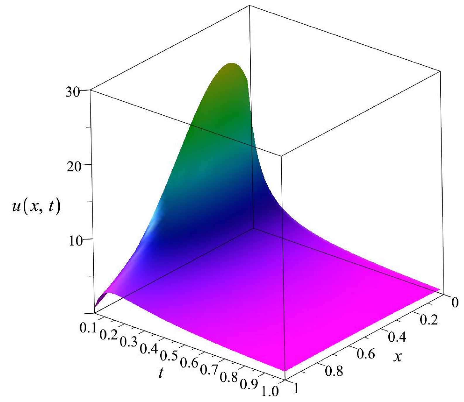
2. Analytical Solution

To solve the PDE (2), we use the well-known reduction technique, where we define a new variable $\eta =\frac{x}{t^{\beta }} \in ℝ$, which is a combination of the spatial and temporal variable. Then we try to find the solution $u\left(x, t\right)$ with the self-similar Ansatz in the form of $u\left(x, t\right)=t^{-\alpha }f\left(x/t^{\beta }\right)$, where α and β are arbitrary real constants, and $f\left(\eta \right)$ is the shape function with existing first and second continuous derivatives with respect to η. Substituting the first and second derivative of the Ansatz into the original Equation (2), we arrive to an ordinary differential equation (ODE) for $f\left(\eta \right)$

$$-\overline{D}{\eta }^m{f}^{″}+f^{\prime }\left(\frac{\eta }{m-2}-\overline{D}m{\eta }^{m-1}\right)-\alpha f=0,$$

if and only if the following constraints are fulfilled for the exponents: α = arbitrary real number, $\beta =\frac{1}{2-m}$, where m is an arbitrary real parameter of the space dependent diffusion coefficient in Equation (2). According to Maple 12 this ODE has the solution

$$\begin{array}{l}f\left(\eta \right)=\frac{c_1}{\sqrt{\eta }}{\mathrm{e}}^{- \frac{{\eta }^{-m+2}}{2\overline{D}{\left(m-2\right)}^2}}\cdot M_{\frac{\left(1+\left(2m-4\right)\alpha \right)\left|m-2\right|}{2{\left(m-2\right)}^2}, \frac{m-1}{2m-4}}\left(\frac{\left|m-2\right|{\eta }^{-m+2}}{{\left(m-2\right)}^3\overline{D}}\right)+\\ \frac{c_2}{\sqrt{\eta }}{\mathrm{e}}^{- \frac{{\eta }^{-m+2}}{2\overline{D}{\left(m-2\right)}^2}}\cdot W_{\frac{\left(1+\left(2m-4\right)\alpha \right)\left|m-2\right|}{2{\left(m-2\right)}^2}, \frac{m-1}{2m-4}}\left(\frac{\left|m-2\right|{\eta }^{-m+2}}{{\left(m-2\right)}^3\overline{D}}\right),\end{array}$$

(3)

where $M$ and $W$ are the Whittaker functions [12,47]. To see the connection to the former results, we note the formulas for expressing the Whittaker functions [12] in terms of the Kummer functions M and U as

$$\begin{array}{l}{M}_{\kappa ,\mu }\left(z\right)={\mathrm{e}}^{-\frac{z}{2}}{z}^{\mu +\frac{1}{2}}M\left(\mu -\kappa +\frac{1}{2},1+2\mu ;z\right)\\ W_{\kappa ,\mu }\left(z\right)={\mathrm{e}}^{-\frac{z}{2}}{z}^{\mu +\frac{1}{2}}U\left(\mu -\kappa +\frac{1}{2},1+2\mu ;z\right).\end{array}$$

(4)

It can be seen from the exponential factor that the Whittaker functions have a quicker decay than the Kummer functions, as we noted in the Introduction. Figure 1 shows the shape functions for various parameters, and Figure 2 exemplifies the time development of the concentration function u for a given parameter set.

3. The Procedure of the Numerical Solution

3.1. The Equation and Its Discretization in the Non-Uniform Case

If the properties of the material depend on space, we can use the following equation:

$$c\left(x\right)\rho \left(x\right)\frac{\partial u}{\partial t}= \frac{\partial }{\partial x}\left(k\left(x\right)\frac{\partial u}{\partial x}\right),$$

(5)

where, in the case of heat conduction, c, ρ, and k are the specific heat, density, and heat conductivity, respectively, and $D=k/(c\rho )$ is the thermal diffusivity. If one differentiates the term $k\left(x\right)\frac{\partial u}{\partial x}$ with respect to x on the right side of (5) considering k as a continuous function, then one obtains a similar equation to (2), where an extra drift term with the first spatial derivative of u appears. To avoid this, we follow another strategy, and discretize the function k, and at the same time the space derivatives in Equation (5) by the standard central difference formula to obtain

$${\left.c(x_i)\rho (x_i)\frac{\partial u}{\partial t}\right|}_{x_i}=\frac{1}{\Delta x} \left[k\left(x_i+\frac{\Delta x}{2}\right)\frac{u(x_i+\Delta x)-u(x_i)}{\Delta x}+k\left(x_i-\frac{\Delta x}{2}\right)\frac{u(x_i-\Delta x)-u(x_i)}{\Delta x}\right].$$

At this point, we switch from node to cell variables. This means that $u_i$, $c_i$, and ${\rho }_i$ are the approximation of the average temperature, specific heat, and density of cell i, by their value at the cell center. Furthermore, $k_{i,i+1}$ is the heat conductivity between cell i and its (right) neighbor, estimated by its value at the border of the cells. Now the previous formula will have the form

$$\frac{d{u}_i}{dt}=\frac{1}{c_i{\rho }_i\Delta x} \left(k_{i,i+1}\frac{u_{i+1}-u_i}{\Delta x}+k_{i-1,i}\frac{u_{i-1}-u_i}{\Delta x}\right).$$

For a non-equidistant grid, let us denote the length of the cell by $\Delta x_i$. The distance between the cell-center of the two neighboring cells as $d_{i, i+1}=\left(\Delta x_i+\Delta x_{i+1}\right)/2$. Using these, the equation above can be generalized as follows:

$$\frac{d{u}_{\mathrm{i}}}{dt}=\frac{1}{c_i{\rho }_i\Delta x_i} \left(k_{i,i+1}\frac{u_{i+1}-u_i}{d_{i,i+1}}+k_{i,i-1}\frac{u_{i-1}-u_i}{d_{i,i-1}}\right).$$

Because we are in one spatial dimension, we consider the cross-section area of the system as unity. Using these quantities, the volume and the heat capacity of the cell can be expressed as $V_i=\Delta x_i$, and $C_i=c_i{\rho }_i\Delta x_i$, respectively, and the thermal resistance between these cells is approximated as $R_{ij}\approx d_{ij}/k_{ij}$. Now we have the equation for the time derivative of each cell-variable:

$$\frac{d{u}_i}{dt}=\frac{u_{i-1}-u_i}{R_{i-1,i}{C}_i}+\frac{u_{i+1}-u_i}{R_{i+1,i}{C}_i},$$

which can be written into a matrix form

$$\frac{d\overrightarrow{u}}{dt}=M\overrightarrow{u},$$

(6)

where the system matrix M is $N\times N$ dimensional. One can find more details about this kind of discretization (for the case of more space dimensions as well) in Chapter 5 of the book [48] and in our previous paper [42].

We implement the power-law space dependence $D=\overline{D} x^m$ of the diffusion coefficient only at the level of the k coefficients, so take $c\equiv 1$ and $\rho \equiv 1$ for simplicity. Let us consider the 1D interval $x\in \left[x_0, x_N\right]$, $L=x_N-x_0$, and we construct a non-equidistant spatial grid using the following procedure. We start with the definition of the coordinates $x_0, x_1, \dots , x_N$ of the cell borders:

$$x_j=x_{j-1}+\Delta x_{j-1}, C_j=\Delta x_j=\Delta x_0\left(1+\gamma j \right) , j=1,\dots ,N.$$

where $x_0$, $\Delta x_0$, and γ will be given in the concrete example. If γ is positive or negative, then the cell sizes are increasing or decreasing from left to right, respectively. If γ is zero, then the grid is equidistant and $L=N\Delta x$. Now the cell centers $X_1, \dots , X_N$ can be given as follows:

$$X_j=x_{j-1}+\frac{\Delta x_j}{2}, j=1,\dots ,N.$$

The resistances are calculated as follows:

$$R_{i, i+1}=\frac{X_{i+1}-X_i}{k_{i, i+1}}=\frac{X_{i+1}-X_i}{\overline{D}{\left(x_i\right)}^m},\hspace{1em}i=1,\dots ,N-1.$$

Therefore, the concentrations, e.g., the Dirichlet boundary conditions, are calculated at the $X_1, \dots , X_N$ cell centers, and the conductivities are calculated at the $x_1, \dots , x_{N-1}$ cell borders. The time variable is always discretized uniformly, so if $t\in \left[t^0, t^{\mathrm{fin}}\right]$, then

$$t^j=t^0+jh, j=1,\dots , T, hT=t^{\mathrm{fin}}-t^0.$$

3.2. The Applied 14 Numerical Algorithms

Here we briefly present necessary information about the used schemes in one space dimension and give the source of the publications where the interested reader can find more details. First, the formula for the simplest case (equidistant mesh and uniform material properties, Equation (1)) is presented, then it is immediately generalized for a non-uniform mesh (Equation (6)). The purpose of the first, simplest form is to make comparison easier, as in most mathematical textbooks and papers numerical algorithms are presented in this form. The second, more general forms are essential because, during our present work, we use only them.

For the case of the general one-dimensional mesh, let us introduce two notations:

$$r_i=\frac{h}{C_i}\left(\frac{1}{R_{i, i-1}}+\frac{1}{R_{i, i+1}}\right) \mathrm{and} A_i=\frac{h}{C_i}\left(\frac{u_{i-1}}{R_{i, i-1}}+\frac{u_{i+1}}{R_{i, i+1}}\right), i=1, \dots ,N.$$

(7)

The first quantity is the generalization of the usual mesh-ratio $r=\frac{Dh}{\Delta x^2}$ valid for Equation (1) if it is discretized using a uniform mesh. The second quantity reflects the state and the effect of the neighbors of cell i.

1. The first invented among our methods is the constant neighbor (CNe) algorithm [45,49]. For a uniform mesh, the following formula must be applied for each node:

$$u_i^{n+1}=u_i^n\cdot e^{- 2r}+\frac{u_{i-1}^n+u_{i+1}^n}{2}\left(1-e^{- 2r}\right),$$

(8)

whereas for non-uniform mesh, the new values of the cell variables are:

$$u_i^{n+1}=u_i^n\cdot e^{- r_{\mathrm{i}}}+\frac{A_i}{r_i}\left(1-e^{- r_{\mathrm{i}}}\right).$$

(9)

2. The CpC algorithm [43] is the organization of the CNe scheme into a two-stage method, in which the first stage is a fractional time step with length ph. Here we use only $p=\raisebox{1ex}{$1$}\!\left/ \!\raisebox{-1ex}{$2$}\right.$, because typically this yields better accuracy than the other values of p. At the first stage, new predictor values of u are calculated with the CNe formula using a $h_1=h/2$ time step size:

$$u_i^{\mathrm{pred}}=u_i^n\cdot e^{- r}+\frac{u_{i-1}^n+u_{i+1}^n}{2}\left(1-e^{- r}\right) \mathrm{and} u_i^{\mathrm{pred}}=u_i^n{e}^{- r_i/2}+\frac{A_i}{r_i}\left(1-e^{- r_i/2}\right).$$

Using these results, new values of the A_i quantities are calculated

$$A_i^{\mathrm{new}}=\frac{h_{ 1}}{C_i}\left(\frac{u_{i-1}^{\mathrm{pred}}}{R_{i, i-1}}+\frac{u_{i+1}^{\mathrm{pred}}}{R_{i, i+1}}\right),$$

(10)

and then, at the second stage, these are used during the full-time step size corrector step. It means that, at the end of the time step, the final values are

$$u_i^{n+1}=u_i^n\cdot e^{- 2r}+\frac{u_{i-1}^{\mathrm{pred}}+u_{i+1}^{\mathrm{pred}}}{2}\left(1-e^{- 2r}\right) \mathrm{and} u_i^{n+1}=u_i^n\cdot e^{- r_{\mathrm{i}}}+\frac{A_i^{\mathrm{new}}}{r_i}\left(1-e^{- r_i}\right).$$

3. The 2-stage linear-neighbor (LNe or LNe2) method [45] starts with using the CNe method as a predictor to calculate new $u_i^{\mathrm{pred}}$ values, which are valid at the end of the current time step. Using them we can introduce a quantity, which is proportional to the aggregated slopes of the neighbors

$$s_i=u_{i-1}^{\mathrm{pred}}+u_{i+1}^{\mathrm{pred}}-u_{i-1}^n-u_{i+1}^n,$$

and then, for the uniform mesh, the corrector values of the two-stage LNe method are

$$u_i^{n+1}=u_i^n{e}^{- 2r}+\frac{u_{i-1}^n+u_{i+1}^n}{2}\left(1-e^{-2r}\right)+\frac{s_i}{2}\left(1-\frac{1-e^{-2r}}{2r}\right).$$

(11)

In the case of a non-uniform mesh, we need to calculate new $A_i^{\mathrm{new}}$ values similarly to Formula (10), but with full h time step size h instead of $h_1$. Using these the corrector step is as follows:

$$u_i^{n+1}=u_i^n{e}^{- r_i}+\left(A_i-\frac{A_i^{\mathrm{new}}-A_i}{r_i}\right)\frac{1-e^{- r_i}}{r_i}+\frac{A_i^{\mathrm{new}}-A_i}{r_i}.$$

(12)

4. Based on the corrector values in Equations (11) or (12), one can repeat (11) or (12)—first by recalculating $s_i$ and $A_i^{\mathrm{new}}$ again—to obtain new corrector results. This procedure gives a three stage-scheme altogether, which is called the LNe3 method [45]. This algorithm is still second order, but more accurate than the LNe2.

5. The CLL method [46] is very similar to the LNe3 method. The difference is that, due to fractional time steps at the first and second stages, it achieves third order temporal convergence, but only if the second fractional time step is $h_2=2h/3$. Generally, the length of the first fractional step is ph, $\raisebox{1ex}{$2$}\!\left/ \!\raisebox{-1ex}{$3$}\right.\le p<2$, but here we take $p=\raisebox{1ex}{$2$}\!\left/ \!\raisebox{-1ex}{$3$}\right.$ to achieve the best accuracy and to spare CPU time by avoiding the extra calculation of the exponential factors $e^{- p{r}_i}$. Therefore, in the first stage, we calculate new predictor values of the variables with the CNe formula, but with a $h_1=2h/3$ time step:

$$u_i^{\mathrm{C}}=u_i^n\cdot e^{-4r/3}+\frac{u_{i-1}^n+u_{i+1}^n}{2}\left(1-e^{-4r/3}\right) \mathrm{and} u_i^{\mathrm{C}}=u_i^n{e}^{- 2r_i/3}+\frac{A_i}{r_i}\left(1-e^{- 2r_i/3}\right).$$

In the second stage, we use formulas similar to (11) and (12), but with an $h_2=2h/3$ time step size to obtain the first corrector values. For the uniform mesh, we have

$$u_i^{n+1}=u_i^n{e}^{-4r/3}+\frac{u_{i-1}^n+u_{i+1}^n}{2}\left(1-e^{-4r/3}\right)+\frac{s_i^1}{2}\left(1-\frac{1-e^{-4r/3}}{4r/3}\right),$$

(13)

where $s_i^1=u_{i-1}^C+u_{i+1}^{\mathrm{C}}-u_{i-1}^n-u_{i+1}^n$. For a non-uniform mesh, we need to calculate new $A_i^{\mathrm{new}}$ values similarly to Formula (10), i.e., $A_i^C=\frac{h_1}{C_i}\left(\frac{u_{i-1}^{\mathrm{C}}}{R_{i, i-1}}+\frac{u_{i+1}^{\mathrm{C}}}{R_{i, i+1}}\right)$. Using these, the corrector step is as follows:

$$u_i^{n+1}=u_i^n{e}^{- 2r_i/3}+\left(A_i-\frac{A_i^{\mathrm{C}}-A_{\mathrm{i}}}{2r_i/3}\right)\frac{1-e^{- 2r_i/3}}{r_i}+\frac{A_i^{\mathrm{C}}-A_i}{r_i}.$$

(14)

In the third stage, a full time step is taken. For the uniform mesh, we have

$$u_i^{n+1}=u_i^n{e}^{-2r}+\frac{u_{i-1}^n+u_{i+1}^n}{2}\left(1-e^{-2r}\right)+\frac{3s_i^2}{4}\left(1-\frac{1-e^{-2r}}{2r}\right),$$

(15)

where $s_i^2=u_{i-1}^{CL}+u_{i+1}^{\mathrm{CL}}-u_{i-1}^n-u_{i+1}^n$. In the more general case, we have

$$u_i^{n+1}=u_i^n{e}^{- r_i}+\left(A_i-\frac{A_i^{\mathrm{CL}}-A_{\mathrm{i}}}{2r_i/3}\right)\frac{1-e^{- r_i}}{r_i}+\frac{A_i^{\mathrm{CL}}-A_i}{2r_i/3},$$

(16)

where $A_i^{\mathrm{CL}}=\frac{h_2}{C_i}\left(\frac{u_{i-1}^{\mathrm{CL}}}{R_{i, i-1}}+\frac{u_{i+1}^{\mathrm{CL}}}{R_{i, i+1}}\right)$.

Now we turn our attention to the odd–even hopscotch methods. To apply any version of them, one needs a bipartite spatial grid, in which all the nearest neighbors of the odd nodes or cells are even and vice versa. The spatial and temporal structure (similar to the stencil) of the examined schemes are presented in Figure 3, where the time flows from the top to the bottom of the figure. In the case of each method, only one odd and one even cell is present in the figure, and the stages are symbolized by colorful boxes. The repeating blocks are indicated by the dashed green line. For example, the leapfrog-hopscotch structure (a) consists of two half and many full time steps. First, a half-sized time step (symbolized by a blue box with the number ‘0′ inside in Figure 3a) is taken for the odd cells using the initial values, then full-time steps are taken strictly alternately for the even and odd cells until the end of the last timestep (pink box), which should be halved for odd cells to reach exactly the same final time as the even nodes do. The main point is that when a new value of u_i is calculated, always the latest values of the neighbors $u_{i\pm 1}$ must be used, which ensures stability and quite fast convergence at the same time.

6. The leapfrog-hopscotch-CNe (LH-CNe) method [13] is obtained if we apply the CNe formula in each stage of the LH structure (Figure 3a) with the appropriate time step size. For example, the first stage (which has half-length on the time axis) reads as follows:

$$u_i^{\raisebox{1ex}{$1$}\!\left/ \!\raisebox{-1ex}{$2$}\right.}=u_i^0\cdot e^{- r}+\frac{u_{i-1}^0+u_{i+1}^0}{2}\left(1-e^{- r}\right) \mathrm{and} u_i^{\raisebox{1ex}{$1$}\!\left/ \!\raisebox{-1ex}{$2$}\right.}=u_i^0\cdot e^{- r_i/2}+\frac{A_i^0}{r_i}\left(1-e^{- r_i/2}\right)$$

whereas the middle stages apply the following formula:

$u_i^{n+1}=u_i^n\cdot e^{- 2r}+\frac{u_{i-1}^{\mathrm{latest}}+u_{i+1}^{\mathrm{latest}}}{2}\left(1-e^{- 2r}\right)$ and $u_i^{n+1}=u_i^n\cdot e^{- r_i}+\frac{A_i^{\mathrm{latest}}}{r_i}\left(1-e^{- r_i}\right)$ for a uniform and a non-uniform mesh, respectively, where the latest values of the neighbors are used to calculate $A_i^{\mathrm{latest}}$ by Formula (10). For the sake of programming simplicity, the total number of cells N of the 1D grid are always odd in our numerical experiments, thus at the first stage, the above formula has been applied for the $i=3 , 5 , 7 , N-2$ cells, and then the boundary conditions have been calculated for the middle of the time intervals for the first and last cell as well.

7. The next method is the leapfrog-hopscotch (LH) method. It uses the so called $\theta$ formula. In our case, this has the form for a uniform mesh:

$$u_i^{n+1}=\frac{\left(1-2r\theta \right)u_i^n+r\left(u_{i-1}^{\mathrm{latest}}+u_{i+1}^{\mathrm{latest}}\right)}{1+2r\left(1-\theta \right)},$$

(17)

and (in the general case),

$$u_i^n=\frac{\left(1-r_i\theta \right)u_i^n+A_i^{\mathrm{latest}}}{1+r_i\left(1-\theta \right)}.$$

(18)

In the paper [13] where it was published, several numerical experiments were conducted, and since then we have been using the formula, which was proven to be the most accurate (labelled with L2 in [13]). It means that $\theta =0$ is applied at the first stage and $\theta =\raisebox{1ex}{$1$}\!\left/ \!\raisebox{-1ex}{$2$}\right.$ in all other stages.

8. In the case of the original odd-even hopscotch algorithm [50], abbreviated by OOEH here, the usual FTCS (explicit Euler) formula was used at the first stage and the implicit Euler formula in the second stage in the structure shown in Figure 3b. The formulas for the uniform and non-uniform mesh are the following:

$$\begin{array}{l}\mathrm{FTCS}: u_i^{n+1}=\left(1-2r\right)u_i^n+r\left(u_{i-1}^n+u_{i+1}^n\right) \mathrm{and} u_i^{n+1}=\left(1-r_i\right)u_i^n+A_i.\\ \mathrm{Implicit} \mathrm{Euler}: u_i^{n+1}=\frac{u_i^n+r\left(u_{i-1}^{n+1}+u_{i+1}^{n+1}\right)}{1+2r} \mathrm{and} u_i^{n+1}=\frac{u_i^n+A_i^{\mathrm{latest}}}{1+r_i}.\end{array}$$

As we showed before [40], this is a powerful explicit method for spatially uniform cases, but if the stiffness ratio is large, its error can be very large [41].

9. The reversed (odd-even) hopscotch method (RH) applies the same structure and the same formulas as the OOEH method, but the formulas are in the opposite order. However, when first-stage calculations start, the new values of the neighbors are not known. Therefore, the implicit formula can be applied only with a trick, which is to handle the neighbors not implicitly, but explicitly. This idea yields the following first-stage formulas:

$$u_i^{n+1}=\frac{u_i^n+r\left(u_{i-1}^n+u_{i+1}^n\right)}{1+2r} \mathrm{and} u_i^{n+1}=\frac{u_i^n+A_i}{1+2r_i}.$$

(19)

If one has the code of the original OOEH, then it is easy to obtain the code of the RH algorithm, as one needs to interchange the formulas of the first and second stages only. We demonstrated [41] that this RH algorithm has much smaller errors in the case of extremely stiff systems than the OOEH method.

10. The shifted-hopscotch (SH) algorithm [42] consists of five stages (two half and three full-time steps). As shown in Figure 3c, these altogether span two full time steps for odd and even cells, as well. In this paper, we use the theta Formulas (17) and (18) with the theta values that are proven to be the best (S4 algorithm in [42]). It means $\theta =0$ is applied at the first, $\theta =\raisebox{1ex}{$1$}\!\left/ \!\raisebox{-1ex}{$2$}\right.$ in the second, third, and fourth, and $\theta =1$ at the fifth stage.

11. The asymmetric-hopscotch (ASH) algorithm [51] is a reduced version of the SH scheme. As shown in Figure 3d, it consists of only three stages (two half and one full-time step), which together span one full time step for odd and even cells, as well. The set of the theta values that is proven to be the best (A1 algorithm in [51]) is $\theta =0$ in the first, $\theta =\raisebox{1ex}{$1$}\!\left/ \!\raisebox{-1ex}{$2$}\right.$ in the second, and $\theta =1$ in the third stage.

12. The pseudo-implicit (PI) two-stage algorithm is taken from [44] (Algorithm 5 there) in the case of the pure diffusion equation with parameter $\lambda =1$, which means we take a half time step to obtain the predictor values and then a full time step for the corrector values. The following formulas must be applied for each cell:

$$\begin{array}{l}Stage 1: u_i^{\mathrm{pred}}=\frac{u_i^n+\raisebox{1ex}{$r$}\!\left/ \!\raisebox{-1ex}{$2$}\right.\left(u_{i-1}^n+u_{i+1}^n\right)}{1+r} \mathrm{and} u_i^{\mathrm{pred}}=\frac{u_i^n+A_i/2}{1+r_i/2}.\\ Stage 2: u_i^{n+1}=\frac{\left(1-r\right)u_i^n+r\left(u_{i-1}^{\mathrm{pred}}+u_{i+1}^{\mathrm{pred}}\right)}{1+r} \mathrm{and} u_i^{n+1}=\frac{\left(1-r_i/2\right)u_i^n+A_i^{\mathrm{new}}}{1+r_i/2},\end{array}$$

where $A_i^{\mathrm{new}}=\frac{h}{C_i}\left(\frac{u_{i-1}^{\mathrm{pred}}}{R_{i, i-1}}+\frac{u_{i+1}^{\mathrm{pred}}}{R_{i, i+1}}\right)$. One can see that the trick of the explicit treatment of the neighbors is the same as in the RH method.

13. The Dufort–Frankel (DF) method [52] (p. 313) is a known but non-conventional explicit and unconditionally stable algorithm that has the formula for the uniform and non-uniform case:

$$u_i^{n+1}=\frac{\left(1-2r\right)u_i^{n-1}+2r\left(u_{i-1}^n+u_{i+1}^n\right)}{1+2r} \mathrm{and} u_i^{n+1}=\frac{\left(1-r_i\right)u_i^{n-1}+2A_i}{1+r_i}.$$

As the formulas contain $u_i^{n-1}$, it is a one-stage but two-step method. It means that $u_i^1$ has to be calculated from $u_i^0$ by another method to start the algorithm. We use the CNe formula for this purpose.

14. For comparison purposes, we use that version of the fourth order Runge–Kutta (RK4) method, which is maybe the most common [53] (p. 737). If we apply it to our spatially discretized system, we have

$$\begin{array}{l}{k}_i^1=r\left(u_{i-1}^n+u_{i+1}^n-2u_i^n, \mathrm{and} k_i^1=A_i-r_i{u}_i^n,\right)\\ k_i^2=r\left(u_{i-1}^n+k_{i-1}^1/2+u_{i+1}^n+k_{i+1}^1/2-2u_i^n-k_i^1, \mathrm{and} k_i^2=A_i^1-r_i\left(u_i^n+k_i^1/2\right),\right)\\ k_i^3=r\left(u_{i-1}^n+k_{i-1}^2/2+u_{i+1}^n+k_{i+1}^2/2-2u_i^n-k_i^2, \mathrm{and} k_i^3=A_i^2-r_i\left(u_i^n+k_i^2/2\right),\right)\\ k_i^4=r\left(u_{i-1}^n+k_{i-1}^3+u_{i+1}^n+k_{i+1}^3-2u_i^n-2k_i^3, \mathrm{and} k_i^4=A_i^3-r_i\left(u_i^n+k_i^3/2\right),\right)\end{array}$$

and finally

$$u_i^{n+1}=u_i^n+\left(k_i^1+2k_i^2+2k_i^3+k_i^4\right)/6.$$

Here $A_i^s=\frac{h}{C_i}\left(\frac{u_{i-1}^n+k_{i-1}^s/2}{R_{i, i-1}}+\frac{u_{i+1}^n+k_{i+1}^s/2}{R_{i, i+1}}\right)$, $s\in \left\{1, 2, 3\right\}$.

Therefore, the CNe, CpC, LNe, LNe3, CLL, LH-CNe, LH, RH, SH, ASH, and PI methods are constructed by our research group and the verifications, analytical proofs, etc. are typically presented in those original papers. The methods are proven to have the following theoretical order of convergence in the time step size. The CNe method is first order, the CpC, LNe, LNe3, CLL, LH-CNe, LH, OOEH, RH, SH, ASH, PI, and DF methods are second order, the CLL method is third order, and the RK4 scheme is fourth order in time step size. All algorithms, (except, of course, the RK4 method) are unconditionally stable for the linear diffusion equation, i.e., the above noted CFL limit is not valid for them. We emphasize again that unconditionally stability is not the rule but the exception among explicit methods, for example, as it is well known, explicit Runge–Kutta methods cannot be A-stable [54] (p. 60).

It is worth noting that the CNe, CpC, LNe, LNe3, and LH-CNe schemes are not only stable but positivity preserving, which sets a limit to their error. More precisely, the new $u_i^{n+1}$ values are the convex combination of the old $u_i^n, u_{i-1}^n, u_{i+1}^n$ etc. values, thus the maximum and minimum principles [55] (p. 87) are automatically fulfilled. This directly reflects the second law of thermodynamics, which states that heat can spontaneously go only from a colder place to a warmer place, which excludes the increase of oscillations in the solutions as time elapses. Thus, these methods do not yield any unphysical oscillations even for very large time step sizes. However, as we will see, this favorable property restricts the speed of the convergence of these methods, so they are often the least accurate for small and medium time step sizes. More concretely, they seriously underestimate the speed of the diffusion process (especially for larger time step sizes), which can be perceived as a “negative” dissipative error.

We also note that the hopscotch-type methods need a special bipartite grid, but in one space dimension this is a trivial requirement. However, these algorithms do not require to temporarily store another copy of the array for the concentration variable, so their memory requirements are minimal. Other methods, even the CNe, store at least one extra array with the same number of elements as u.

4. Numerical Results

4.1. Preliminaries

To measure the accuracy, we use the usual $L_{\infty }$ error, which is the largest absolute difference between the exact value of the concentration $u_i^{\mathrm{analytic}}$ and $u_i^{\mathrm{num}}$ obtained by the studied numerical method at the final time $t^{\mathrm{fin}}$:

$$Error=\underset{1\le i\le N}{\max }\left|u_i^{\mathrm{analytic}}(t^{\mathrm{fin}})-u_i^{\mathrm{num}}(t^{\mathrm{fin}})\right|.$$

(20)

We examine this error as a function of the time step size h. For this purpose, we first calculate the error for a very large h, then repeat this with decreased time step sizes until we reach small error values. From Figure 3, one can see that the SH and the ASH structure are obtained by halving a time step to the odd nodes. This might be considered as a hidden extra advantage given to these methods. Therefore, for the sake of honesty and to make comparisons easier, we renormalize their time step size, i.e., we introduce the effective time step size, which is

$$h_{\mathrm{eff}}=\raisebox{1ex}{$4$}\!\left/ \!\raisebox{-1ex}{$5$}\right.h \mathrm{for} \mathrm{the} \mathrm{SH}, h_{\mathrm{eff}}=\raisebox{1ex}{$2$}\!\left/ \!\raisebox{-1ex}{$3$}\right.h \mathrm{for} \mathrm{the} \mathrm{ASH} \mathrm{and} h_{\mathrm{eff}}=h \mathrm{for} \mathrm{all} \mathrm{other} \mathrm{methods}.$$

(21)

With this modification, the CNe, LH-CNe, LH, OOEH, RH, SH, ASH, and DF methods require only one calculation of A_i and the new u values of the cells in a given time step, so they have the highest speed. The CpC, LNe2, and PI need two calculations ($A_i^{\mathrm{new}}$ and $u_i^{\mathrm{pred}}$ must also be calculated), so their running time is roughly twice larger. The required number of calculations is three for the LNe3 and the CCL, whereas it is obviously four for the RK4 method, so they are approximately proportionally slower. We note that there are plenty of data about the running times of the recent methods in our original papers.

In all numerical experiments we use the following parameters:

$$\overline{D}=1 , \alpha =1.5 , N=199 , c_1=1 , c_2=0t^0=0.5t^{\mathrm{fin}}=0.6.$$

(22)

All other parameters can vary in concrete cases. It means that we are going to reproduce the following reference solution:

$$C\left(x,t\right)=t^{-\frac{3}{2}}f\left(\frac{x}{t^{\beta }}\right) = \sqrt{\frac{t^{\beta -3}}{x}}\cdot {\mathrm{e}}^{- \frac{{\left(\frac{x}{t^{\beta }}\right)}^{-m+2}}{2{\left(m-2\right)}^2}}\cdot M_{\frac{\left(1+3\left(m-2\right)\right)\left|m-2\right|}{2{\left(m-2\right)}^2}, \frac{m-1}{2m-4}}\left(\frac{\left|m-2\right|{\left(\frac{x}{t^{\beta }}\right)}^{-m+2}}{{\left(m-2\right)}^3}\right).$$

(23)

MATLAB software has been used to do all numerical calculations, where the Kummer M function (confluent hypergeometric function of the first kind) has been calculated via the command hypergeom. We note that calculating the two values of the boundary conditions for a given time point is four orders of magnitude slower than performing the numerical steps for all the 199 nodes of the grid.

All the eigenvalues of the system matrix M are negative. The stiffness ratio of the problem can be defined as ${\lambda }_{\mathrm{MAX}}/{\lambda }_{\mathrm{MIN}}$, where ${\lambda }_{\mathrm{MIN}} \left({\lambda }_{\mathrm{MAX}}\right)$ are the smallest (largest) absolute value eigenvalues of M. However, there are threshold time step sizes $h_{\mathrm{MAX}}^{\mathrm{FTCS}}=\left|2/{\lambda }_{\mathrm{MAX}}\right|$ and $h_{\mathrm{MAX}}^{\mathrm{RK}4} \approx \left|2.8/{\lambda }_{\mathrm{MAX}}\right|$ (frequently called CFL limits), above which the solutions by FTCS (explicit Euler) and RK4 schemes, respectively, are expected to blow up [54].

4.2. Spatially Uniform Grid, γ = 0

Experiment 1: We use an equidistant grid with $\Delta x=0.01$, $x\in \left[0.1 , 2.09\right]$, and we set m = 3.6. For this problem, $h_{\mathrm{MAX}}^{\mathrm{FTCS}}=3.9\cdot {10}^{-6}$ and the stiffness ratio is $2.6\cdot {10}^6$. In Figure 4, the errors as a function of the time step size are shown in a log–log diagram. Because we use a fixed space step size and decrease only the time step size, the errors cannot go to zero, but only to the residual error due to space discretization, which can be seen in the bottom left of the figure.

We calculated the numerical order of convergence using two values of the errors belonging to two subsequent time step sizes using the formula

$$Error\sim h^p \Rightarrow \hspace{1em}p=\frac{\log \frac{Error\left(h_1\right)}{Error\left(h_2\right)}}{\log \left(h{ }_1/h_2\right)}.$$

In

Table 1. Errors and numerical order of different algorithms for Experiment 1.

Numerical Method	Error (L∞)	Numerical Order
$\mathrm{CNe}, h=8.12\cdot {10}^{-6}$	$3.03\cdot {10}^{-2}$	1.00
$\mathrm{CNe}, h=4.07\cdot {10}^{-6}$	$1.52\cdot {10}^{-2}$
$\mathrm{CpC}, h=8.12\cdot {10}^{-6}$	$5.2\cdot {10}^{-3}$	1.77
$\mathrm{CpC}, h=4.07\cdot {10}^{-6}$	$1.5\cdot {10}^{-3}$
$\mathrm{LNe}, h=8.12\cdot {10}^{-6}$	$6.0\cdot {10}^{-3}$	1.75
$\mathrm{LNe}, h=4.07\cdot {10}^{-6}$	$1.8\cdot {10}^{-3}$
$\mathrm{LNe}3, h=8.12\cdot {10}^{-6}$	$1.7\cdot {10}^{-3}$	2.42
$\mathrm{LNe}3, h=4.07\cdot {10}^{-6}$	$3.2\cdot {10}^{-4}$
$\mathrm{CLL}, h=8.12\cdot {10}^{-6}$	$9.1\cdot {10}^{-4}$	2.53
$\mathrm{CLL}, h=4.07\cdot {10}^{-6}$	$1.6\cdot {10}^{-4}$
$\mathrm{LH}-\mathrm{CNe}, h=8.12\cdot {10}^{-6}$	$3.0\cdot {10}^{-3}$	1.98
$\mathrm{LH}-\mathrm{CNe}, h=4.07\cdot {10}^{-6}$	$7.6\cdot {10}^{-4}$
$\mathrm{PI}, h=8.12\cdot {10}^{-6}$	$5.0\cdot {10}^{-3}$	1.65
$\mathrm{PI}, h=4.07\cdot {10}^{-6}$	$1.6\cdot {10}^{-4}$
$\mathrm{LH}, h=0.0021$	$4.7\cdot {10}^{-2}$	2.62
$\mathrm{LH}, h=0.0010$	$7.6\cdot {10}^{-3}$
$\mathrm{OOEH}, h=0.0021$	1.36	2.33
$\mathrm{OOEH}, h=0.0010$	0.27
$\mathrm{RH}, h=0.0021$	1.38	2.22
$\mathrm{RH}, h=0.0010$	0.30
$\mathrm{SH}, h=0.0021$	0.30	2.28
$\mathrm{SH}, h=0.0010$	$6.1\cdot {10}^{-2}$
$\mathrm{ASH}, h=0.0021$	0.30	2.28
$\mathrm{ASH}, h=0.0010$	$6.1\cdot {10}^{-2}$
$\mathrm{DF}, h=0.0021$	0.14	1.67
$\mathrm{DF}, h=0.0010$	$4.5\cdot {10}^{-2}$

, we present numerical order for one pair of neighboring error quantities (one section of the curves in Figure 4) with the values of the errors for each method.

We also plotted the initial and final concentrations for the CLL and LH methods with different time step size in Figure 5, where the errors are approximately the same, namely 0.0483 for the CLL method ($h=6.5\cdot {10}^{-5}$) and 0.0465 for the LH method (h = 0.0021). In Figure 6, the $u\left(x,t\right)$ functions are presented in the form of 3D surfaces for the analytical and one numerical solution. One can see that the two surfaces are indistinguishable by the naked eye. Finally, in Figure 7, we present the function $u^{\mathrm{analytic}}(t, x)-u^{\mathrm{num}}(t, x)$, i.e., the difference between the analytical solution and the LH method for h = 0.0021 as a function of space and time in a 3D plot to help the readers to visualize how the error is developing in time.

Experiment 2: In this example, we shift the space interval to $x\in \left[4 , 5.99\right]$, while we keep the values of Equation (22) and those of the previous experiment: $\Delta x=0.01$, m = 3.6. For this problem, $h_{\mathrm{MAX}}^{\mathrm{FTCS}}=8.3\cdot {10}^{-8}$, and the stiffness ratio is $1.2\cdot {10}^7$. From Figure 8, one can see that now the errors start to significantly decrease (with decreasing h) only below $h={10}^{-3}$ instead of $h={10}^{-2}$ as in Figure 4. In contrast, the errors finally tend to much smaller values for the best methods. However, the RK4 method is practically useless, as it is unstable even for $h=5\cdot {10}^{-7}$ and therefore it is missing from the figure. The errors of some methods and the appropriate numerical orders are tabulated in

Table 2. Errors and numerical order of different algorithms for Experiment 2.

Numerical Method	Error (L∞)	Numerical Order
$\mathrm{CNe}, h=4.1\cdot {10}^{-6}$	$4.9\cdot {10}^{-3}$	1.14
$\mathrm{CNe}, h=2.0\cdot {10}^{-6}$	$2.2\cdot {10}^{-3}$
$\mathrm{LNe}, h=4.1\cdot {10}^{-6}$	$2.3\cdot {10}^{-3}$	1.18
$\mathrm{LNe}, h=2.0\cdot {10}^{-6}$	$1.0\cdot {10}^{-3}$
$\mathrm{CLL}, h=4.1\cdot {10}^{-6}$	$1.0\cdot {10}^{-3}$	1.22
$\mathrm{CLL}, h=2.0\cdot {10}^{-6}$	$4.3\cdot {10}^{-4}$
$\mathrm{LH}, h=1.3\cdot {10}^{-4}$	$3.3\cdot {10}^{-5}$	2.49
$\mathrm{LH}, h=6.5\cdot {10}^{-5}$	$5.8\cdot {10}^{-6}$
$\mathrm{OOEH}, h=1.3\cdot {10}^{-4}$	$7.1\cdot {10}^{-3}$	2.00
$\mathrm{OOEH}, h=6.5\cdot {10}^{-5}$	$1.8\cdot {10}^{-3}$
$\mathrm{DF}, h=1.3\cdot {10}^{-4}$	$3.5\cdot {10}^{-4}$	3.39
$\mathrm{DF}, h=6.5\cdot {10}^{-5}$	$3.3\cdot {10}^{-5}$

. In Figure 9, we plotted the functions u for the LH and the DF method with a different time step size, where the errors are approximately the same, namely $7.0\cdot {10}^{-4}$ for the LH method ($h=5.2\cdot {10}^{-4}$), and $7.2\cdot {10}^{-4}$ for the DF method ($h=2.6\cdot {10}^{-4}$). In Figure 10, we present the difference between the analytical solution and the LH method for $h=5.2\cdot {10}^{-4}$ as a function of space and time in a 3D plot to help the readers to visualize how the error is developing in time.

Experiment 3: Here we fix the time step size to $h=5\cdot {10}^{-4}$ and vary the parameter m. The following parameters have been set as $\Delta x=0.015$, $x\in \left[4 , 5.99\right]$, and of course, we keep the values given in Equation (22). The errors are plotted in Figure 11. For simplicity, we disregard the usage of effective time step sizes for the SH and ASH methods, and, due to that, their curves are very close to each other. One can see that the good performance of the LH and the DF methods is not an accident but a general trend. The RK4 method is completely missing from the figure as it never provided any meaningful value for this time step size.

4.3. Spatially Non-Equidistant Grid

Experiment 4: Now we set $\gamma =-0.003$, m = 3.6, $x_0=0.1$, and $\Delta x_0=0.012$, thus the last cell length is $\Delta x_N=0.0048$ and its center is at $X_N=1.7692$. For this problem, $h_{\mathrm{MAX}}^{\mathrm{FTCS}}=1.7\cdot {10}^{-6}$, and the stiffness ratio is $5.8\cdot {10}^6$. In Figure 12, one can see that the error-functions are very similar to those in Figure 4, which means that the methods work well for the non-equidistant case as well. Some errors and the calculated numerical orders are presented in

Table 3. Errors and numerical order of different algorithms for Experiment 3.

Numerical Method	Error (L∞)	Numerical Order
$\mathrm{CNe}, h=8.1\cdot {10}^{-6}$	$4.1\cdot {10}^{-2}$	1.03
$\mathrm{CNe}, h=4.1\cdot {10}^{-6}$	$2.0\cdot {10}^{-2}$
$\mathrm{LNe}, h=8.1\cdot {10}^{-6}$	$1.1\cdot {10}^{-2}$	1.66
$\mathrm{LNe}, h=4.1\cdot {10}^{-6}$	$3.4\cdot {10}^{-3}$
$\mathrm{CLL}, h=8.1\cdot {10}^{-6}$	$2.4\cdot {10}^{-3}$	2.24
$\mathrm{CLL}, h=4.1\cdot {10}^{-6}$	$5.1\cdot {10}^{-4}$
$\mathrm{LH}, h=2.1\cdot {10}^{-3}$	$7.2\cdot {10}^{-2}$	3.00
$\mathrm{LH}, h=1.0\cdot {10}^{-3}$	$9.0\cdot {10}^{-3}$
$\mathrm{OOEH}, h=2.1\cdot {10}^{-3}$	4.45	1.90
$\mathrm{OOEH}, h=1.0\cdot {10}^{-3}$	1.19
$\mathrm{DF}, h=2.1\cdot {10}^{-3}$	0.18	1.31
$\mathrm{DF}, h=1.0\cdot {10}^{-3}$	$7.2\cdot {10}^{-2}$

. In Figure 13, the deviations of the numerical solution from the analytical one is shown as a function of space and time.

Experiment 5: Now we set $\gamma =0.04$ to obtain a mesh where the length of the cells is rapidly increasing with x. We choose m = 7.2, $x_0=0.3$, and $\Delta x_0=0.004$, thus the last cell length is $\Delta x_N=0.0358$, and its center is at $X_N=4.262$. For this problem, $h_{\mathrm{MAX}}^{\mathrm{FTCS}}=2.3\cdot {10}^{-8}$, and the stiffness ratio is $9.1\cdot {10}^8$.

In Figure 14, the error functions are presented. The errors of six numerical schemes and the numerical orders are presented in

Table 4. Errors and numerical order of different algorithms for Experiment 5.

Numerical Method	Error (L∞)	Numerical Order
$\mathrm{CNe}, h=2.6\cdot {10}^{-4}$	$3.7\cdot {10}^{-2}$	0.87
$\mathrm{CNe}, h=1.3\cdot {10}^{-4}$	$2.0\cdot {10}^{-2}$
$\mathrm{LNe}, h=2.6\cdot {10}^{-4}$	$1.3\cdot {10}^{-2}$	1.31
$\mathrm{LNe}, h=1.3\cdot {10}^{-4}$	$5.0\cdot {10}^{-3}$
$\mathrm{CLL}, h=2.6\cdot {10}^{-4}$	$4.4\cdot {10}^{-3}$	1.56
$\mathrm{CLL}, h=1.3\cdot {10}^{-4}$	$1.5\cdot {10}^{-3}$
$\mathrm{LH}, h=1.7\cdot {10}^{-2}$	$8.3\cdot {10}^{-2}$	1.81
$\mathrm{LH}, h=8.3\cdot {10}^{-3}$	$2.4\cdot {10}^{-3}$
$\mathrm{SH}, h=2.1\cdot {10}^{-3}$	$3.6\cdot {10}^{-2}$	3.08
$\mathrm{SH}, h=1.0\cdot {10}^{-3}$	$4.2\cdot {10}^{-3}$
$\mathrm{DF}, h=8.3\cdot {10}^{-3}$	$7.9\cdot {10}^{-2}$	2.10
$\mathrm{DF}, h=4.2\cdot {10}^{-3}$	$1.8\cdot {10}^{-2}$

. One can see that even the least accurate CNe method beats the RK4 scheme, as CNe reaches the minimum error at about $h=3\cdot {10}^{-6}$, whereas RK4 can be stable only below $h\approx 3.2\cdot {10}^{-8}$, at an almost two orders of magnitude smaller time step size. We are going to examine the reason for this.

In Figure 15, we plot the functions u for the CNe and the SH method with a different time step size, where the errors are comparable, namely, 0.02 for the CNe method ($h=1.3\cdot {10}^{-4}$), and 0.036 for the SH method ($h=0.0021$).

We can see that there are two completely different types of difficulties in this problem. As one can see on the left-hand side of Figure 11, the function u is changing rapidly for small values of x. For x < 1, the quickly converging methods, such as the OOEH, LH, SH, ASH, and OOEH, approximate the true solution quite well, whereas other methods, especially the CNe, lag behind. The other difficulty can be understood if one calculates the resistances: they are decreasing from $R_{1,2}=22.3$ to $R_{198,199}=1.2\cdot {10}^{-6}$, thus the right side of the problem yields extremely large (negative) eigenvalues. The tiny CFL limit for the conditionally stable RK methods is caused by this right side, where actually nothing interesting happens from the physical point of view, as the function is very flat and changes almost nothing. This is a fatal weakness of the conventional RK methods and causes trouble, albeit to a much smaller extent, to the SH and other otherwise rapidly converging schemes. In the case of the RK and those hopscotch-type methods that are not unconditionally positive, unphysical oscillations appear, but in the unconditionally stable cases, these oscillations are damped and never grow unbounded. This damping is very effective for the LH method, and that is why it is more accurate than the positivity preserving CpC and LNe3 methods, even for large time step sizes. For the OOEH, RH, SH, and ASH schemes, this damping is not very effective for large time step sizes; it is only enough to keep them stable, that is why their error is rather large on the right-hand side of Figure 4, Figure 8, Figure 12 and Figure 14. Another difference is that the LH method produces the largest oscillations on the left side, where the true function is changing rapidly, whereas the RH, SH, and ASH methods do it at the right side. To illustrate this, in Figure 16, we have plotted the difference $u_i^{\mathrm{analytic}}(t^{\mathrm{fin}})-u_i^{\mathrm{num}}(t^{\mathrm{fin}})$ cell by cell as a function of the x variable for four different methods. The time- development of the error is presented in Figure 17 for the CLL method.

5. Discussion and Summary

We have constructed a set of novel analytical solutions for the non-steady-state linear diffusion equation using a similarity transformation for the case when the diffusion coefficient depends on the space coordinate. The solution is a linear combination of the Whittaker functions, thus it is highly nontrivial.

We have reproduced the new analytical solution by 14 numerical methods, one of which is the most standard fourth order Runge–Kutta method, and the rest are explicit and unconditionally stable schemes, most of them recently invented. First, we have used a spatially uniform (equidistant) mesh, then a non-uniform one, where $\Delta x$ changed smoothly. We observed that usually the leapfrog-hopscotch method has the best performance and the Dufort–Frankel has the second best. However, if unconditional positivity is essential, the LNe3 method can be used. Nevertheless, all of the unconditionally stable explicit methods give accurate results for orders-of-magnitude larger time step size than the standard explicit methods. Therefore, we encourage scholars who still use the explicit RK method for the simulation of linear diffusion or heat conduction problems to switch to an unconditionally stable explicit method. If the diffusion is nonlinear or contains extra terms (convection or reaction), more investigation of these schemes is still necessary. That is why we consider this study as a precursor of subsequent investigations in which we analyze concentration dependent (nonlinear) diffusion equations as well as reaction–diffusion equations of different types, e.g., the FitzHugh–Nagumo [56], the Allen [57], and the Burgers–Huxley equation [58]. Reaction–diffusion equations come into play in numerous scientific fields, such as mathematical biology [59], plasma physics, or even social sciences. We are going to use the Ansatz to obtain new analytical solutions, then adapt some of the most efficient methods (especially the LH) to these cases. We note that a few of our methods have already been applied to Fisher’s equation with good results, so we believe in the successful continuation.

References

1. Lienhard, J.H., IV; Lienhard, J.H., V. A Heat Transfer Textbook, 4th ed.; Phlogiston Press: Cambridge, MA, USA, 2017; ISBN 9780971383524. [Google Scholar]
2. Jacobs, M.H. Diffusion Processes; Springer: Berlin/Heidelberg, Germany, 1935; ISBN 978-3-642-86414-8. [Google Scholar]
3. Zwanzig, R. Diffusion past an entropy barrier. J. Phys. Chem. 1992, 96, 3926–3930. [Google Scholar] [CrossRef]
4. Reguera, D.; Rubí, J.M. Kinetic equations for diffusion in the presence of entropic barriers. Phys. Rev. E-Stat. Phys. Plasmas Fluids Relat. Interdiscip. Top. 2001, 64, 8. [Google Scholar] [CrossRef] [PubMed] [Green Version]
5. Wolfson, M.; Liepold, C.; Lin, B.; Rice, S.A. A comment on the position dependent diffusion coefficient representation of structural heterogeneity. J. Chem. Phys. 2018, 148, 194901. [Google Scholar] [CrossRef] [PubMed]
6. Berezhkovskii, A.; Hummer, G. Single-file transport of water molecules through a carbon nanotube. Phys. Rev. Lett. 2002, 89, 064503. [Google Scholar] [CrossRef] [PubMed]
7. Kärger, J.; Ruthven, D.M. Diffusion in Zeolites and other Microporous Solids; Wiley: New York, NY, USA, 1992; 605p, ISBN 0-471-50907-8. [Google Scholar]
8. Hille, B. Ion Channels of Excitable Membranes, 3rd ed.; Oxford University Press Inc.: New York, NY, USA, 2001; ISBN 9780878933211. [Google Scholar]
9. Mátyás, L.; Barna, I.F. General Self-Similar Solutions of Diffusion Equation and Related Constructions. Rom. J. Phys. 2022, 67, 101. [Google Scholar]
10. Bluman, G.; Cole, J. The General Similarity Solution of the Heat Equation. J. Math. Mech. 1969, 18, 1025–1042. [Google Scholar]
11. Zoppou, C.; Knight, J.H. Analytical solution of a spatially variable coefficient advection-diffusion equation in up to three dimensions. Appl. Math. Model. 1999, 23, 667–685. [Google Scholar] [CrossRef]
12. Olver, F.W.J.; Lozier, D.W.; Boisvert, R.F.; Clark, C.W. NIST Handbook of Mathematical Functions; Cambridge Univ. Press: New York, NY, USA, 2011; Volume 66, ISBN 978-0-521-14063-8. [Google Scholar]
13. Nagy, Á.; Omle, I.; Kareem, H.; Kovács, E.; Barna, I.F.; Bognar, G. Stable, Explicit, Leapfrog-Hopscotch Algorithms for the Diffusion Equation. Computation 2021, 9, 92. [Google Scholar] [CrossRef]
14. Savović, S.M.; Djordjevich, A. Numerical solution of diffusion equation describing the flow of radon through concrete. Appl. Radiat. Isot. 2008, 66, 552–555. [Google Scholar] [CrossRef]
15. Suárez-Carreño, F.; Rosales-Romero, L. Convergency and stability of explicit and implicit schemes in the simulation of the heat equation. Appl. Sci. 2021, 11, 4468. [Google Scholar] [CrossRef]
16. Lima, S.A.; Kamrujjaman, M.; Islam, M.S. Numerical solution of convection-diffusion-reaction equations by a finite element method with error correlation. AIP Adv. 2021, 11, 085225. [Google Scholar] [CrossRef]
17. Ivanovic, M.; Svicevic, M.; Savovic, S. Numerical solution of Stefan problem with variable space grid method based on mixed finite element/finite difference approach. Int. J. Numer. Methods Heat Fluid Flow 2017, 27, 2682–2695. [Google Scholar] [CrossRef]
18. Appau, P.O.; Dankwa, O.K.; Brantson, E.T. A comparative study between finite difference explicit and implicit method for predicting pressure distribution in a petroleum reservoir. Int. J. Eng. Sci. Technol. 2019, 11, 23–40. [Google Scholar] [CrossRef] [Green Version]
19. Moncorgé, A.; Tchelepi, H.A.; Jenny, P. Modified sequential fully implicit scheme for compositional flow simulation. J. Comput. Phys. 2017, 337, 98–115. [Google Scholar] [CrossRef]
20. Chou, C.S.; Zhang, Y.T.; Zhao, R.; Nie, Q. Numerical methods for stiff reaction-diffusion systems. Discret. Contin. Dyn. Syst.-Ser. B 2007, 7, 515–525. [Google Scholar] [CrossRef]
21. Zhang, J.; Zhao, C. Sharp error estimate of BDF2 scheme with variable time steps for molecular beam expitaxial models without slop selection. J. Math. 2021, 41, 1–19. [Google Scholar]
22. Amoah-mensah, J.; Boateng, F.O.; Bonsu, K. Numerical solution to parabolic PDE using implicit finite difference approach. Math. Theory Model. 2016, 6, 74–84. [Google Scholar]
23. Mbroh, N.A.; Munyakazi, J.B. A robust numerical scheme for singularly perturbed parabolic reaction-diffusion problems via the method of lines. Int. J. Comput. Math. 2022, 99, 1139–1158. [Google Scholar] [CrossRef]
24. Aminikhah, H.; Alavi, J. An efficient B-spline difference method for solving system of nonlinear parabolic PDEs. SeMA J. 2018, 75, 335–348. [Google Scholar] [CrossRef]
25. Ali, I.; Haq, S.; Nisar, K.S.; Arifeen, S.U. Numerical study of 1D and 2D advection-diffusion-reaction equations using Lucas and Fibonacci polynomials. Arab. J. Math. 2021, 10, 513–526. [Google Scholar] [CrossRef]
26. Singh, M.K.; Rajput, S.; Singh, R.K. Study of 2D contaminant transport with depth varying input source in a groundwater reservoir. Water Sci. Technol. Water Supply 2021, 21, 1464–1480. [Google Scholar] [CrossRef]
27. Ji, Y.; Zhang, H.; Xing, Y. New Insights into a Three-Sub-Step Composite Method and Its Performance on Multibody Systems. Mathematics 2022, 10, 2375. [Google Scholar] [CrossRef]
28. Gagliardi, F.; Moreto, M.; Olivieri, M.; Valero, M. The international race towards Exascale in Europe. CCF Trans. High Perform. Comput. 2019, 1, 3–13. [Google Scholar] [CrossRef] [Green Version]
29. Reguly, I.Z.; Mudalige, G.R. Productivity, performance, and portability for computational fluid dynamics applications. Comput. Fluids 2020, 199, 104425. [Google Scholar] [CrossRef]
30. Appadu, A.R. Performance of UPFD scheme under some different regimes of advection, diffusion and reaction. Int. J. Numer. Methods Heat Fluid Flow 2017, 27, 1412–1429. [Google Scholar] [CrossRef] [Green Version]
31. Karahan, H. Unconditional stable explicit finite difference technique for the advection-diffusion equation using spreadsheets. Adv. Eng. Softw. 2007, 38, 80–86. [Google Scholar] [CrossRef]
32. Sanjaya, F.; Mungkasi, S. A simple but accurate explicit finite difference method for the advection-diffusion equation. J. Phys. Conf. Ser. 2017, 909, 012038. [Google Scholar] [CrossRef]
33. Pourghanbar, S.; Manafian, J.; Ranjbar, M.; Aliyeva, A.; Gasimov, Y.S. An efficient alternating direction explicit method for solving a nonlinear partial differential equation. Math. Probl. Eng. 2020, 2020, 9647416. [Google Scholar] [CrossRef]
34. Harley, C. Hopscotch method: The numerical solution of the Frank-Kamenetskii partial differential equation. Appl. Math. Comput. 2010, 217, 4065–4075. [Google Scholar] [CrossRef]
35. Al-Bayati, A.; Manaa, S.; Al-Rozbayani, A. Comparison of Finite Difference Solution Methods for Reaction Diffusion System in Two Dimensions. AL-Rafidain J. Comput. Sci. Math. 2011, 8, 21–36. [Google Scholar] [CrossRef] [Green Version]
36. Nwaigwe, C. An Unconditionally Stable Scheme for Two-Dimensional Convection-Diffusion-Reaction Equations. 2022. Available online: https://www.researchgate.net/publication/357606287_An_Unconditionally_Stable_Scheme_for_Two-Dimensional_Convection-Diffusion-Reaction_Equations (accessed on 5 August 2022).
37. Savović, S.; Drljača, B.; Djordjevich, A. A comparative study of two different finite difference methods for solving advection–diffusion reaction equation for modeling exponential traveling wave in heat and mass transfer processes. Ric. Mat. 2021, 71, 245–252. [Google Scholar] [CrossRef]
38. Ndou, N.; Dlamini, P.; Jacobs, B.A. Enhanced Unconditionally Positive Finite Difference Method for Advection–Diffusion–Reaction Equations. Mathematics 2022, 10, 2639. [Google Scholar] [CrossRef]
39. Saleh, M.; Nagy, Á.; Kovács, E. Part 1: Construction and investigation of new numerical algorithms for the heat equation. Multidiszcip. Tudományok 2020, 10, 323–338. [Google Scholar] [CrossRef]
40. Saleh, M.; Nagy, Á.; Kovács, E. Part 2: Construction and investigation of new numerical algorithms for the heat equation. Multidiszcip. Tudományok 2020, 10, 339–348. [Google Scholar] [CrossRef]
41. Saleh, M.; Nagy, Á.; Kovács, E. Part 3: Construction and investigation of new numerical algorithms for the heat equation. Multidiszcip. Tudományok 2020, 10, 349–360. [Google Scholar] [CrossRef]
42. Nagy, Á.; Saleh, M.; Omle, I.; Kareem, H.; Kovács, E. New stable, explicit, shifted-hopscotch algorithms for the heat equation. Math. Comput. Appl. 2021, 26, 61. [Google Scholar] [CrossRef]
43. Kovács, E.; Nagy, Á.; Saleh, M. A set of new stable, explicit, second order schemes for the non-stationary heat conduction equation. Mathematics 2021, 9, 2284. [Google Scholar] [CrossRef]
44. Jalghaf, H.K.; Kovács, E.; Majár, J.; Nagy, Á.; Askar, A.H. Explicit stable finite difference methods for diffusion-reaction type equations. Mathematics 2021, 9, 3308. [Google Scholar] [CrossRef]
45. Kovács, E. A class of new stable, explicit methods to solve the non-stationary heat equation. Numer. Methods Partial Differ. Equ. 2020, 37, 2469–2489. [Google Scholar] [CrossRef]
46. Kovács, E.; Nagy, Á.; Saleh, M. A New Stable, Explicit, Third-Order Method for Diffusion-Type Problems. Adv. Theory Simul. 2022, 5, 2100600. [Google Scholar] [CrossRef]
47. Wikipedia Whittaker Function. Available online: https://en.wikipedia.org/wiki/Whittaker_function (accessed on 5 August 2022).
48. Munka, M.; Pápay, J. 4D Numerical Modeling of Petroleum Reservoir Recovery; Akadémiai Kiadó: Budapest, Hungary, 2001; ISBN 963-05-7843-3. [Google Scholar]
49. Kovács, E. New Stable, Explicit, First Order Method to Solve the Heat Conduction Equation. J. Comput. Appl. Mech. 2020, 15, 3–13. [Google Scholar] [CrossRef]
50. Gourlay, A.R.; McGuire, G.R. General Hopscotch Algorithm for the Numerical Solution of Partial Differential Equations. IMA J. Appl. Math. 1971, 7, 216–227. [Google Scholar] [CrossRef]
51. Saleh, M.; Kovács, E. New Explicit Asymmetric Hopscotch Methods for the Heat Conduction Equation. In Proceedings of the 1st International Electronic Conference on Algorithms, Online, 27 September–10 October 2021; MDPI: Basel, Switzerland, 2021; Volume 2, p. 22. [Google Scholar]
52. Hirsch, C. Numerical Computation of Internal and External Flows, Volume 1: Fundamentals of Numerical Discretization; Wiley: Hoboken, NJ, USA, 1988. [Google Scholar]
53. Chapra, S.C.; Canale, R.P. Numerical Methods for Engineers, 7th ed.; McGraw-Hill Science/Engineering/Math: New York, NY, USA, 2015. [Google Scholar]
54. Iserles, A. A First Course in the Numerical Analysis of Differential Equations; Cambridge Univ. Press: Cambridge, UK, 2009; ISBN 9788490225370. [Google Scholar]
55. Holmes, M.H. Introduction to Numerical Methods in Differential Equations; Springer: New York, NY, USA, 2007; ISBN 978-0387-30891-3. [Google Scholar]
56. Agbavon, K.M.; Appadu, A.R. Construction and analysis of some nonstandard finite difference methods for the FitzHugh–Nagumo equation. Numer. Methods Partial Differ. Equ. 2020, 36, 1145–1169. [Google Scholar] [CrossRef]
57. Sabawi, Y.A.; Ahmed, S.B.; Hamad, H.Q. Numerical Treatment of Allen’s Equation Using Semi Implicit Finite Difference Methods. Eurasian J. Sci. Eng. 2022, 8, 90–100. [Google Scholar] [CrossRef]
58. Verma, A.K.; Kayenat, S. An efficient Mickens’ type NSFD scheme for the generalized Burgers Huxley equation. J. Differ. Equ. Appl. 2020, 26, 1213–1246. [Google Scholar] [CrossRef]
59. Alba-Pérez, J.; Macías-Díaz, J.E. A finite-difference discretization preserving the structure of solutions of a diffusive model of type-1 human immunodeficiency virus. Adv. Differ. Equ. 2021, 2021, 158. [Google Scholar] [CrossRef]
Figure 1. Shape functions of Equation (3) in the case of generalized space-dependent diffusion coefficients for various values of α with different m exponents of the diffusion parameter: (A) α = 2 , (B) α = 1 , (C) α = 1 2 , (D) α = 1 , (E) α = 3 2 , (F) α = 5 2 . The real part of the solutions is presented for D ¯ = 1 , c 1 = 0 , c 2 = 1 . The black, red, blue, green, brown, grey, and yellow lines are for m = 1   ,   1 2   ,   0 ,   1 2   ,   1   ,   3 2     ,   and   5 2 , respectively.
Mathematics 10 02813 g001
Figure 2. The solution of Equation (2). The presented u(x, t) function with the shape function of Equation (3) is for the α = 1, c1 = 0, c2 = 1, D ¯ = 2 and m = 1/3 parameter set. One can see that the solution decays more quickly in time than in space.
Mathematics 10 02813 g002
Figure 3. Space-time structure of the hopscotch-type methods. (a) Leapfrog-hopscotch (LH), (b) original odd-even hopscotch (OOEH), (c) shifted-hopscotch (SH), (d) asymmetric hopscotch (ASH).
Mathematics 10 02813 g003
Figure 4. Errors as a function of the effective time step size heff for Experiment 1. The errors are defined in (20), and heff is defined in (21). The slopes of the error curves give the order of convergence of the methods.
Mathematics 10 02813 g004
Figure 5. The concentration u as a function of the x variable in the case of the initial function u0, the analytical solution at t fin , the CLL method for h = 6.5 10 5 , and the leapfrog-hopscotch (LH) method for h = 0.0021 for Experiment 1. We emphasize that the conventional Runge–Kutta methods are unstable for these time step sizes.
Mathematics 10 02813 g005
Figure 6. The concentration u as a function of x and t in the case of Experiment 1. Left side: the analytical solution. Right side: LH method for h = 0.0021.
Mathematics 10 02813 g006
Figure 7. The difference between the analytical solution and the LH method for h = 0.0021 as a function of space and time for Experiment 1.
Mathematics 10 02813 g007
Figure 8. The L errors as a function of the time step size h for an equidistant mesh for large x (Experiment 2). RK4 is not present in the figure because it is unstable for the examined time step sizes, as the CFL limit for the standard RK4 method is approximately h 1.2 10 7 .
Mathematics 10 02813 g008
Figure 9. The concentration u as a function of the x variable in the case of the initial function u0, the analytical solution at t fin , the LH method for h = 5.2 10 4 , and the DF method for h = 2.6 10 4 in the case of Experiment 2. The LH and the DF curves almost coincide.
Mathematics 10 02813 g009
Figure 10. The function u analytic ( t ,   x ) u num ( t ,   x ) , i.e., the difference between the analytical solution and the LH method for h = 5.2 10 4 as a function of space and time for Experiment 2.
Mathematics 10 02813 g010
Figure 11. The L errors as a function of the parameter m for an equidistant mesh (Experiment 3). RK4 is not present in the figure because it is unstable for the examined time step size.
Mathematics 10 02813 g011
Figure 12. The L errors as a function of the time step size h for a decreasing mesh (Experiment 4).
Mathematics 10 02813 g012
Figure 13. The difference between the analytical solution and the LH method for h = 2.1 10 3 as a function of space and time for Experiment 4.
Mathematics 10 02813 g013
Figure 14. The L errors as a function of the time step size h for a decreasing mesh (Experiment 5). RK4 is not present in the figure because it is unstable for the examined time step sizes, as it is stable only below h 3.2 10 8 .
Mathematics 10 02813 g014
Figure 15. The concentration u as a function of the x variable in the case of the initial function u0, the analytical solution at t fin , the CNe method for h = 1.3 10 4 , and the SH method for h = 2.1 10 3 . The SH curve almost coincides with the exact one for small values of x, whereas this is true for the CNe curve for large x. The CFL limit for the standard RK4 method is approximately h 3.2 10 8 .
Mathematics 10 02813 g015
Figure 16. The errors of the cell concentrations as a function of the x variable in the case of the CLL and the SH method for h = 10 3 , and the LH and DF method h = 4.2 10 3 .
Mathematics 10 02813 g016
Figure 17. The difference between the analytical solution and the CLL method for h = 1.0 10 3 as a function of space and time for Experiment 5.
Mathematics 10 02813 g017