
Partially Coupled Stochastic Gradient Estimation for Multivariate Equation-Error Systems


1
Jiangsu Key Laboratory of Media Design and Software Technology, School of Artificial Intelligence and Computer Science, Jiangnan University, Wuxi 214122, China
2
School of Automation, Wuxi University, Wuxi 214105, China
*
Author to whom correspondence should be addressed.
Mathematics 2022, 10(16), 2955; https://doi.org/10.3390/math10162955
Submission received: 5 July 2022
/
Revised: 4 August 2022
/
Accepted: 12 August 2022
/
Published: 16 August 2022
(This article belongs to the Section Engineering Mathematics)
Abstract
:This paper researches the identification problem for the unknown parameters of the multivariate equation-error autoregressive systems. Firstly, the original identification model is decomposed into several sub-identification models according to the number of system outputs. Then, based on the characteristic that the information vector and the parameter vector are common among the sub-identification models, the coupling identification concept is used to propose a partially coupled generalized stochastic gradient algorithm. Furthermore, by expanding the scalar innovation of each subsystem model to the innovation vector, a partially coupled multi-innovation generalized stochastic gradient algorithm is proposed. Finally, the numerical simulations indicate that the proposed algorithms are effective and have good parameter estimation performances.
Keywords:
parameter estimation; coupling identification; stochastic gradient; multi-innovation theory; multivariate systemMSC:
93C351. Introduction
Parameter estimation is an important part in the field of system identification, which usually identifies the unknown parameters in the models according to the input and output data of the system when the model structure of a system is known [1,2,3]. Parameter estimation has been used in many fields in recent years, including chemistry, mechanics, engineering and so on [4,5,6]. For example, in chemical engineering field, Khalik et al. applied the parameter estimation approach by using current/voltage data in achieving physically meaningful parameters of the Doyle–Fuller–Newman model for Lithium-ion batteries [7]. In mechanics field, Shamrao et al. estimated the terramechanics parameters by applying dynamic Bayesian estimation techniques on the measurements from simple single-wheel tests [8]. In engineering, Calasan et al. proposed two algorithms for the transformer parameter estimation to improve the estimation process and prevent inaccuracies and parameter mismatch with the real parameters of the transformer [9].
In many identification objects of parameter estimation, multivariate systems is a very common class [10,11,12]. The majority of industrial processes are the multivariate systems [13,14]. It is not easy to estimate the unknown parameters of multivariate systems, because such systems are quite complex; for example, there are many variables, there is coupling between variables, or there is time delay [15,16,17]. In recent years, the identification of the multivariate systems has attracted the attention of many scholars. Shafin et al. studied the angle and delay estimation for 3D massive MIMO systems under a parametric channel modeling, which was crucial for such systems to realize the predicted capacity gains [18]. Kawaria et al. designed a Levy shuffled frog leaping algorithm with high parameter estimation efficiency to estimate the parameters of multiple-input–multiple-output bilinear systems [19]. Roy et al. developed an online plant-parameter identification method for the multi-input–multi-output linear time-invariant systems [20].
The coupling identification concept is a useful identification method that has been developed in recent decades. It is suitable for parameter estimation problems for the multivariate systems with the same parameters among subsystems [21,22]. The identification algorithm based on the coupling concept has the advantage of lower computation amounts compared with the traditional identification algorithm for multivariate systems. Cui et al. combined the Kalman filtering principle and the coupling identification concept to derive a Kalman filtering-based partially coupled recursive least squares algorithm for jointly estimating the parameters and the states of the multivariable state–space system; their algorithm had high computational efficiency [23]. The multi-innovation identification theory is also an effective method that has been used to improve parameter estimation accuracy in recent years [24,25,26]. This method not only utilizes the data information of the current time, but also makes full use of the data information of the previous time [27,28,29]. Chaudhary et al. presented a multi-innovation fractional least mean square adaptive algorithm for the input-nonlinear systems by expanding the scalar innovation into a vector innovation by using the multi-innovation identification theory [30]. This method can also be applied to the parameter estimation of the multivariate systems.
We have studied the parameter identification problems of multivariate systems in the past. In [31], the colored noise of the original system was filtered into white noise by using the data filtering technique. In [32], the original identification system was decomposed into two sub-identification systems, where one contains the system model parameter vector and the other contains the noise model parameter matrix by applying the decomposition method. However, the coupling identification concept used in this paper is different from the previous two identification methods, as it decomposes the original system according to the number of system outputs to obtain several subsystems with partial parameter vectors and information vectors coupled. It has significant advantages in reducing the computational cost of the algorithm because it makes the original complex system simplified. Therefore, this paper presents new identification methods to estimate the parameters of the multivariate equation-error autoregressive system, which have high computational efficiency and high parameter estimation accuracy. The main contributions of this paper lie in the following.
- This paper decomposes the multivariate equation-error autoregressive system into several sub-identification models according to the number of the system outputs.
- A multivariate partially coupled generalized stochastic gradient (M-PC-GSG) algorithm is proposed for the multivariate equation-error system by utilizing the coupling identification concept, which can reduce the computation amounts compared with the traditional stochastic gradient algorithm.
- A multivariate partially coupled multi-innovation generalized stochastic gradient (M-PC-MI-GSG) algorithm is proposed by using the multi-innovation identification theory, which has higher parameter estimation accuracy than the M-PC-GSG algorithm.
The rest of this paper is organized as follows. Section 2 presents a multivariate equation-error autoregressive system and describes its identification difficulties. Section 3 proposes a partially coupled generalized stochastic gradient algorithm and gives its schematic diagram. Section 4 proposes a partially coupled multi-innovation generalized stochastic gradient algorithm. Section 5 presents two numerical examples to indicate that the proposed algorithms are effective. Finally, we offer some concluding remarks in Section 6.
2. System Description and Identification Model
First of all, we give some notation in this paper. denotes an identity matrix of size ; stands for an n-dimensional column vector whose elements are 1, that is ; represents a matrix of size whose elements are 1; the norm of a matrix is defined by , the superscript T stands for the matrix/vector transpose, the symbol ⊗ represents Kronecker product, for example, , , , in general, ; is defined as a vector consisting of all columns of matrix arranged in order, for example, , , ,,⋯,.
Consider the following multivariate equation-error autoregressive system,
where is the system output vector, is the system information matrix consisting of the input-output data, is the system parameter vector to be identified, ,,⋯, is a white noise process with zero mean, is a polynomial matrix in the unit backward shift operator :
Define the noise model,
Assume that the orders m, n and are known, and , , and for .
Define the parameter matrix and the information vector as
From Equation (2), we have
Then, the multivariate equation-error autoregressive system in (1) can be transformed into the following identification model,
For the identification model in (5), the objective of this paper is to identify the unknown parameters and by researching some identification methods. Currently, the observable data are and . Certainly, the most direct identification method is to integrate the information vector and the information matrix into a new information matrix , and the parameter matrix and the parameter vector into a new parameter matrix , then we can obtain the following identification model:
However, the information matrix in model (6) contains a large number of zero elements because it is calculated from the Kronecker product, which results in redundant computation amounts in the identification processes. Therefore, it is necessary to find an alternative method with less computation amounts to estimate the identification model in (5). In this paper, two efficient algorithms with good performances are proposed to solve this problem by applying the coupling identification concept and the multi-innovation identification theory.
Suppose that is the estimate of at time t. That is to say , and are estimates of , and at time t, respectively.
3. The Partially Coupled Stochastic Gradient Algorithm
First of all, according to the number of the system outputs, decomposing the identification model in (5) into m sub-identification models:
where are the ith row of the parameter matrix , and are the ith row of the information matrix :
For the m sub-identification models in (9), it can be seen that the information vector and the parameter vector are common among the m subsystems. Thus, Equation (5) is a coupling identification model of partial parameter vectors and partial information vectors. Equation (9) can be represented as
Assuming that and are the step-size, using the negative gradient search [33] and minimizing , we have the gradient relationships:
The problem of identification in (11)–(14) is that the estimates and can not be computed because contains the unmeasurable noise terms . The method to solve this problem is to replace the unmeasurable variables with their corresponding estimates . Thus, the estimate of can be computed by :
It can be seen that the parameter vector is estimated for m times in (11) and (12), which will lead to many redundant estimates. Using the estimate to replace the estimate in (11) can reduce the redundant computation. At the same time, replacing the unknown information vector with its estimate , we can obtain the new gradient relationships:
Additionally, according to Equations (4), we have
It is generally believed that the parameter estimate of the th subsystem at time t is closer to the true value than the parameter estimate of the ith subsystem at time . Replacing on the right-hand of Equation (16) with , and replacing of Equation (16) when with . Combing Equations (15) and (20), we can obtain the multivariate partially coupled generalized stochastic gradient (M-PC-GSG) algorithm as
4. The Partially Coupled Multi-Innovation Stochastic Gradient Algorithm
In this section, we apply the multi-innovation identification theory based on the M-PC-GSG algorithm to further improve the parameter estimation accuracy. We introduce an innovation length to expand the innovation scalars of each subsystem models to the innovation vectors. According to the M-PC-GSG algorithm in (21)–(32), define the subsystem stacked information matrices , , and the subsystem stacked output vectors and as
According to the multi-innovation identification theory, expand the subsystem innovation scalars and into the subsystem innovation vectors and :
Normally, we reach an agreement that the estimates and at time are closer to the true values and than the estimates and at time . Similarly, the estimate at time t is closer to the true value than the estimate at time . Therefore, replacing the terms , and () with , and in (33) and (34), and the subsystem innovation vectors and are modified into
Thus, based on the the M-PC-GSG algorithm in (21)–(32), we can obtain the following multivariate partially coupled multi-innovation generalized stochastic gradient (M-PC-MI-GSG) algorithm with an innovation length p:
- Let , choose an innovation length p, set the initial values , , , , , , 1, ⋯, , , and set the data length K.
- Collect the observation data and , read from using (52).
- Construct using (53).
- Compute using (41).
- Compute using (48).
- Increase t by 1 if , and then go to Step 2. Otherwise, obtain parameter estimates and and stop computing.
It can be easily seen that the M-PC-MI-GSG algorithm with the innovation length is equal to the M-PC-GSG algorithm. Since the past data information of the system are utilized sufficiently, the M-PC-MI-GSG algorithm has higher parameter estimation accuracy than the M-PC-GSG algorithm.
5. The Simulation Examples
In this section, two numerical simulations are given to show the good performances of the newly proposed algorithms.
Example 1.
Consider the following multivariate equation-error autoregressive systems,
The parameter vector to be estimated is
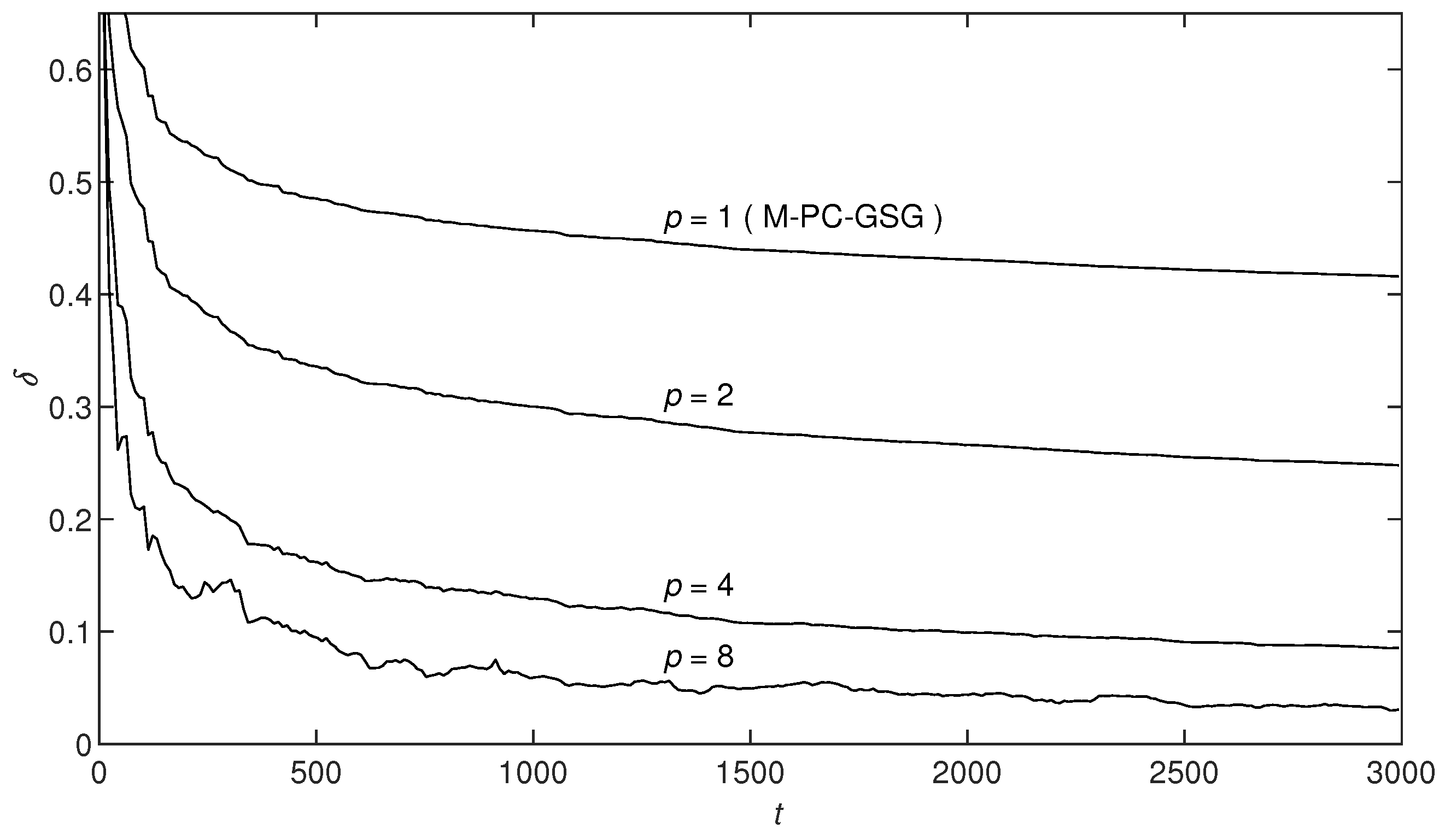
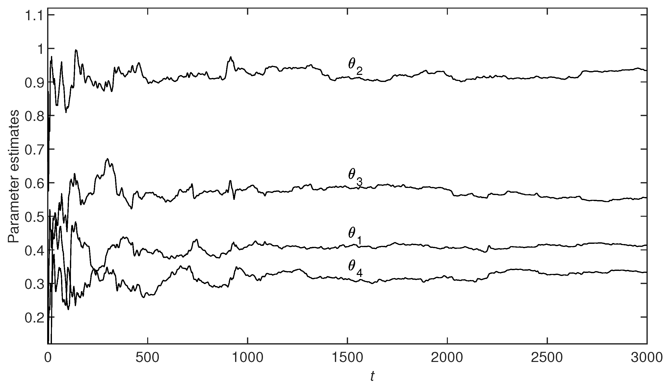
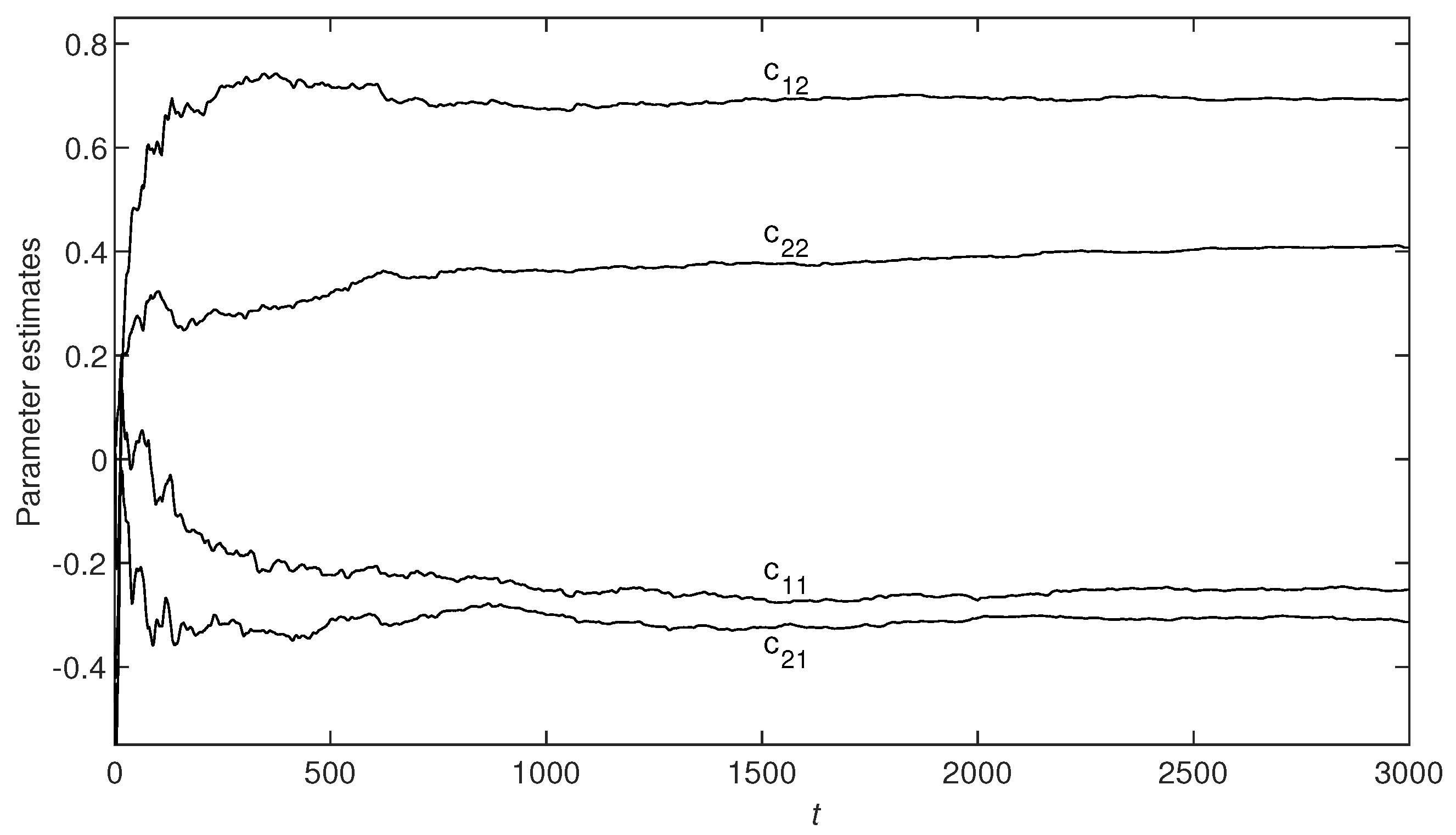
In this simulation, is the input vector, which is a random sequence with zero mean and variance one; is the output vector; is a white noise vector with zero mean; and are the variances of and . Taking the noise variances and , using the M-PC-GSG algorithm (i.e., the M-PC-MI-GSG algorithm with ) and the M-PC-MI-GSG algorithm with , and to estimate the parameters of this example system. We obtain the parameter estimates and their errors shown in Table 1. The parameter estimation errors versus t are shown in Figure 2. The parameter estimates , , , and , , , versus t of the M-PC-MI-GSG algorithm with are shown in Figure 3 and Figure 4.
Example 2.
Consider another multivariate equation-error autoregressive systems,
The parameter vector to be estimated is
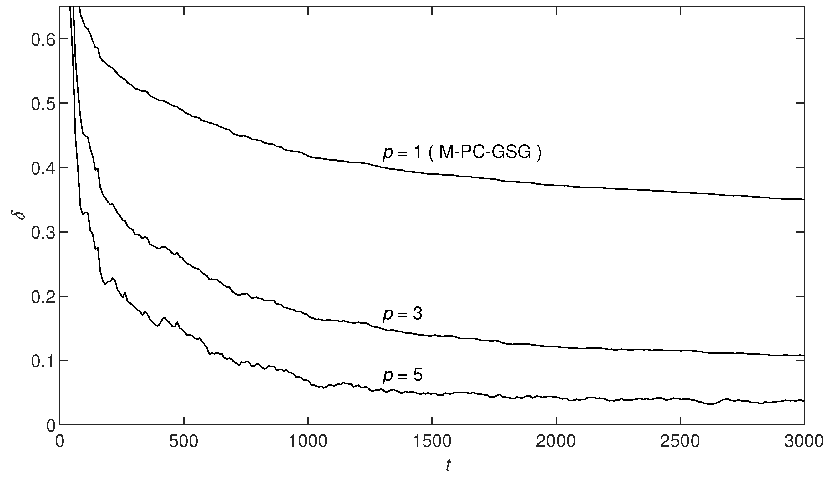
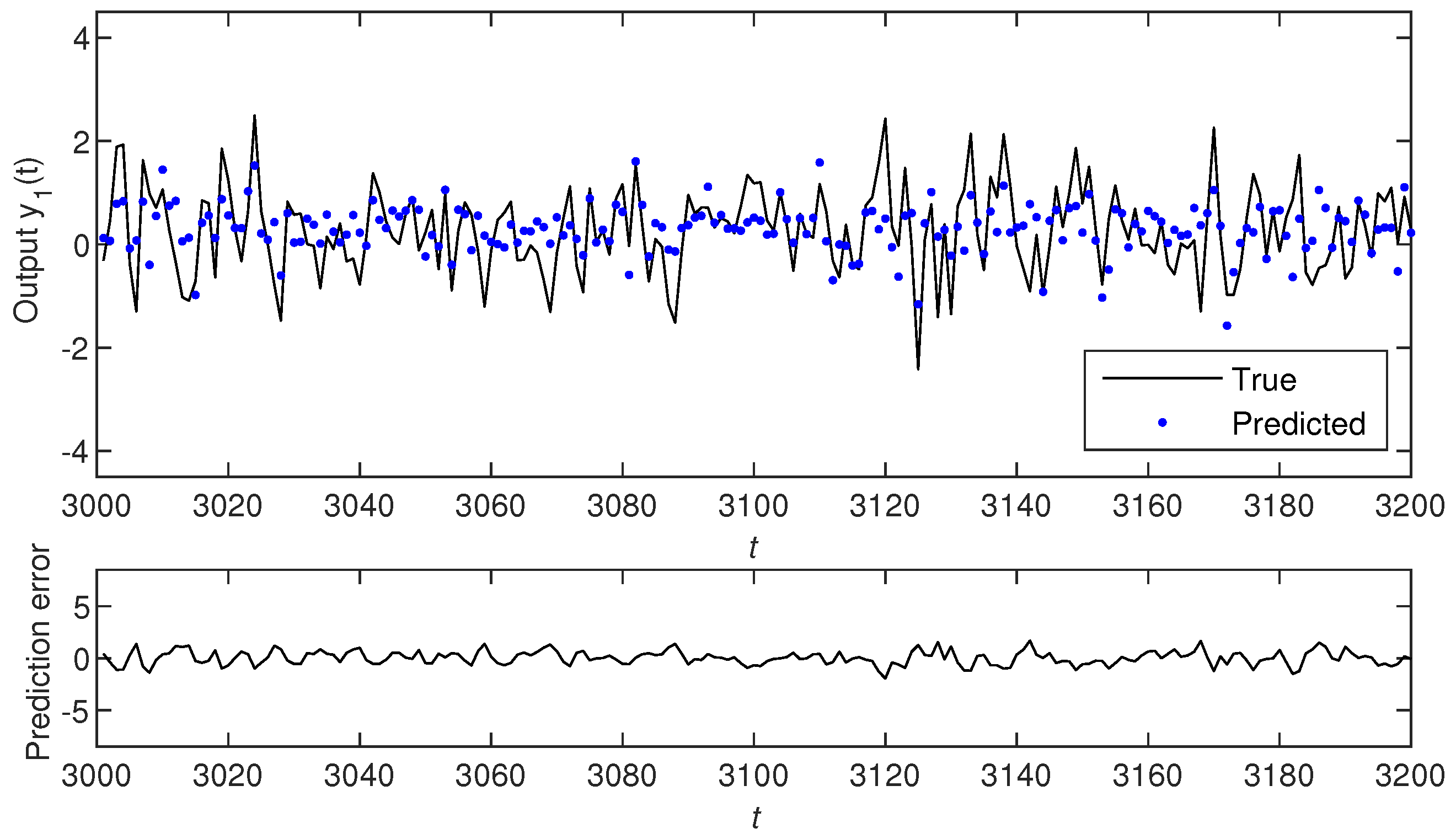
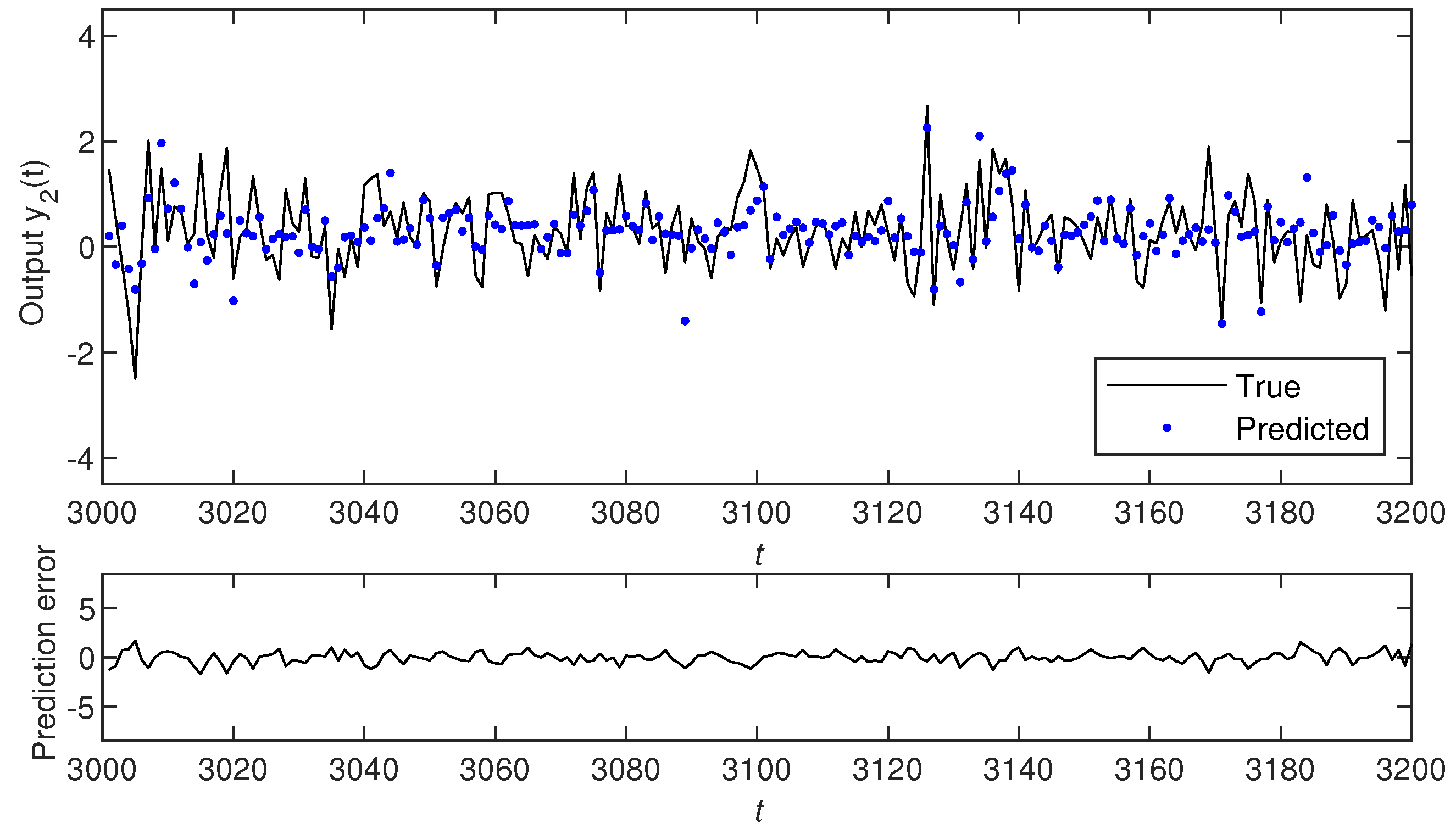
Here, the simulation conditions are similar to Example 1. Taking the noise variances , using the M-PC-GSG algorithm (i.e., the M-PC-MI-GSG algorithm with ) and the M-PC-MI-GSG algorithm with and to estimate the parameters of this example system. The parameter estimates and their errors are shown in Table 2. The parameter estimation errors versus t are shown in Figure 5. For model validation, we use the estimated model obtained by the M-PC-MI-GSG algorithm with to predict the system outputs with 200 samples from to . The true output and the predicted output as well as their errors are shown in Figure 6. The true output and the predicted output as well as their errors are shown in Figure 7.
From Table 1 and Table 2 and Figure 2, Figure 3, Figure 4, Figure 5, Figure 6 and Figure 7, the following conclusions are obtained.
- From Table 1 and Table 2, Figure 2 and Figure 5, it can be shown that the parameter estimation errors of the M-PC-GSG and the M-PC-MI-GSG algorithms become smaller as the data length t increases, which means that the proposed algorithms are effective in parameter estimation for the multivariate autoregressive system.
- Figure 2 and Figure 5 show that the M-PC-MI-GSG algorithm has higher parameter estimation accuracy than the M-PC-GSG algorithm under the same noise variances and same data length. Introducing the innovation length p can effectively improve the parameter estimation accuracy for the M-PC-GSG algorithm, and the parameter estimates can be more stationary as the innovation length p increases.
Remark 1.
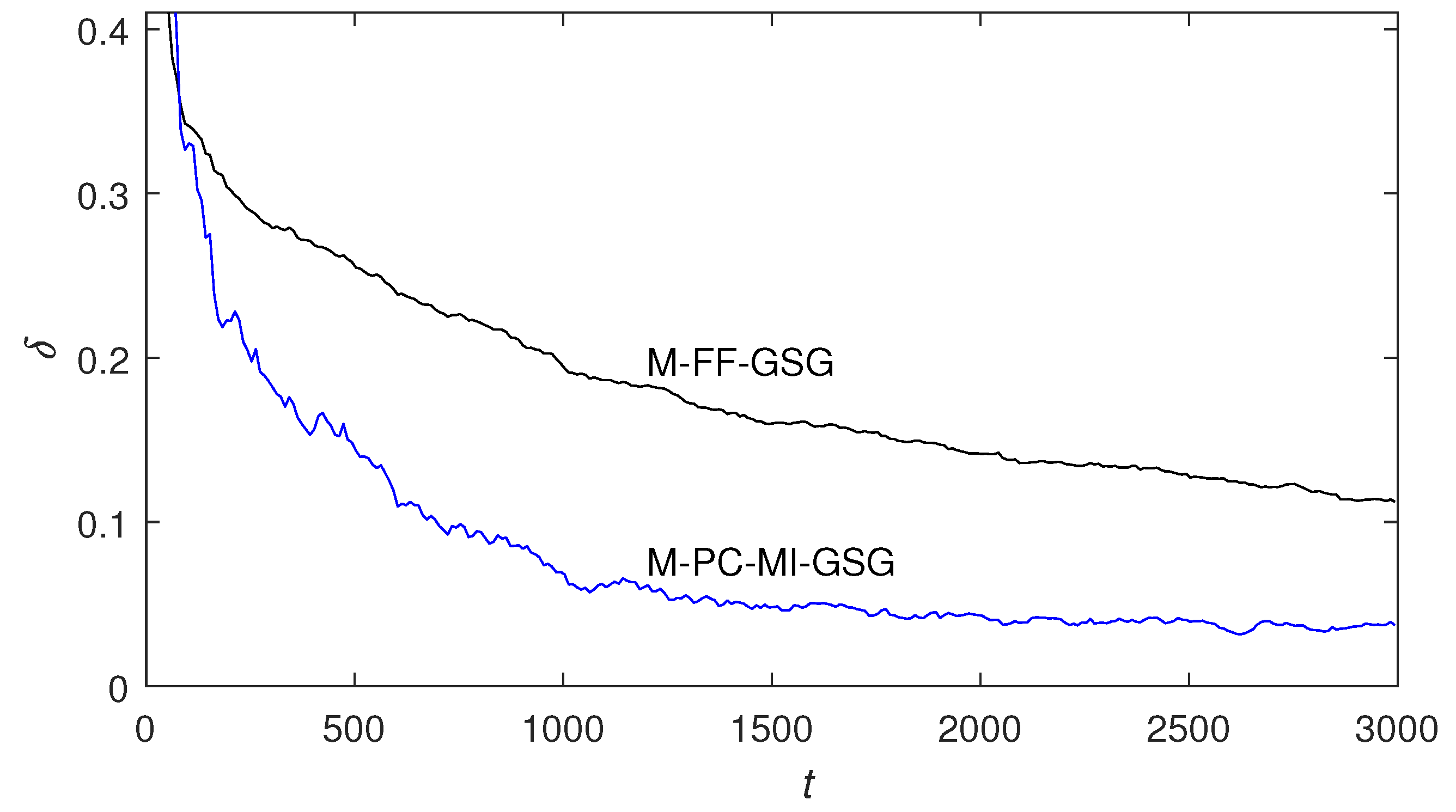
In order to show the advantages of the identification performances of the proposed algorithm in this paper, the forgetting factor stochastic gradient identification method proposed in [34] is compared with the proposed algorithm. The forgetting factor stochastic gradient identification method is applied to identify the multivariate equation-error autoregressive systems in this paper, and the multivariate forgetting factor generalized stochastic gradient (M-FF-GSG) algorithm is obtained. The M-FF-GSG algorithm is compared with the M-PC-MI-GSG algorithm with through simulation, and the simulation experimental conditions are the same as those in Example 2. The comparison results are shown in Figure 8. It can be seen that the proposed algorithm in this paper has faster identification speed and higher estimation accuracy.
6. Conclusions
Coupling identification concept is an emerging method in the field of system identification in recent decades, one which is usually used in the parameter estimation of the multivariate systems. Its main idea is to utilize the parameter-coupling characteristic, and to identify the parameter of each subsystem model separately and then connected, which can greatly reduce the calculation amounts in the estimation processes. This paper combines the coupling identification concept with the stochastic gradient identification method to propose a new identification algorithm for multivariate equation-error systems. The proposed algorithm has the advantage of a lower computation than the traditional stochastic gradient identification algorithm. Additionally, the multi-innovation identification theory is also a promising identification method, which makes full use of the data information collected in the past to identify the unknown parameters. Based on the partially coupled stochastic gradient algorithm, this paper then introduces the innovation length by applying the multi-innovation identification theory, and proposes the partially coupled multi-innovation stochastic gradient algorithm. The new algorithm also has the advantage of higher parameter estimation accuracy.
The proposed coupling and multi-innovation-based identification methods can be extended to study other multivariate systems with different structures and disturbance noises. Meanwhile, the idea of the algorithms can be utilized when the system identification model has the coupled terms. The future research opportunities are to apply the proposed algorithms to actual engineering production systems to improve the computational efficiency and accuracy of the system identification in production practice. Additionally, the proposed methods in the paper can also combine other mathematical tools and statistical strategies to research the performances of some parameter estimation algorithms for other linear or nonlinear systems with colored noises.
Author Contributions
Writing—original draft, P.M.; Writing—review and editing, L.W. All authors have read and agreed to the published version of the manuscript.
Funding
This work was supported by the National Natural Science Foundation of China (No. 61873111), the Fundamental Research Funds for the Central Universities (No. JUSRP121071), the Natural Science Foundation of the Higher Education Institutions of Jiangsu Province (No. 22KJB120009), and the Start-up Fund for Introducing Talent of Wuxi University (No. 2021r045).
Institutional Review Board Statement
Not applicable.
Informed Consent Statement
Not applicable.
Data Availability Statement
All data generated or analyzed during this study are included in this article.
Conflicts of Interest
The authors declare no conflict of interest.
Abbreviations
The following abbreviations are used in this manuscript:
| Abbreviations | Explanations |
| M-PC-GSG | the multivariate partially coupled generalized stochastic gradient algorithm |
| M-PC-MI-GSG | the multivariate partially coupled multi-innovation generalized stochastic |
| gradient algorithm | |
| M-FF-GSG | the multivariate forgetting factor generalized stochastic gradient algorithm |
References
- Na, J.; Yang, J.; Wu, X.; Guo, Y. Robust adaptive parameter estimation of sinusoidal signals. Automatica 2015, 53, 376–384. [Google Scholar] [CrossRef]
- Wang, J.; Efimov, D.; Bobtsov, A.A. On robust parameter estimation in finite-time without persistence of excitation. IEEE Trans. Autom. Control 2020, 65, 1731–1738. [Google Scholar] [CrossRef]
- Xu, L. Application of the Newton iteration algorithm to the parameter estimation for dynamical systems. J. Comput. Appl. Math. 2015, 288, 33–43. [Google Scholar] [CrossRef]
- Mo, D.; Duarte, M.F. Compressive parameter estimation via K-median. Signal Process. 2018, 142, 36–48. [Google Scholar] [CrossRef]
- Demirli, R.; Saniie, J. Asymmetric Gaussian chirplet model and parameter estimation for generalized echo representation. J. Frankl. Inst. 2014, 351, 907–921. [Google Scholar] [CrossRef]
- Upadhyay, R.K.; Paul, C.; Mondal, A.; Vishwakarma, G.K. Estimation of biophysical parameters in a neuron model under random fluctuations. Appl. Math. Comput. 2018, 329, 364–373. [Google Scholar] [CrossRef]
- Khalik, Z.; Donkers, M.C.F.; Sturm, J.; Bergveld, H.J. Parameter estimation of the Doyle-Fuller-Newman model for Lithium-ion batteries by parameter normalization, grouping, and sensitivity analysis. J. Power Sources 2021, 499, 229901. [Google Scholar] [CrossRef]
- Padmanabhan, C.; Gupta, S.; Mylswamy, A. Estimation of terramechanics parameters of wheel-soil interaction model using particle filtering. J. Terramechanics 2018, 79, 79–95. [Google Scholar]
- Calasan, M.P.; Jovanovic, A.; Rubezic, V.; Mujicic, D.; Deriszadeh, A. Notes on parameter estimation for single-phase transformer. IEEE Trans. Ind. Appl. 2020, 56, 3710–3718. [Google Scholar] [CrossRef]
- Zhang, X.; El Korso, M.N.; Pesavento, M. MIMO radar target localization and performance evaluation under SIRP clutter. Signal Process. 2017, 130, 217–232. [Google Scholar] [CrossRef]
- Kulikova, M.V.; Tsyganova, J.V.; Kulikov, G.Y. UD-based pairwise and MIMO kalman-like filtering for estimation of econometric model structures. IEEE Trans. Autom. Control 2020, 65, 4472–4479. [Google Scholar] [CrossRef]
- Weijtjens, W.; Sitter, G.D.; Devriendt, C.; Guillaume, P. Operational modal parameter estimation of MIMO systems using transmissibility functions. Automatica 2014, 50, 559–564. [Google Scholar] [CrossRef]
- Wang, H.; Xu, L.W.; Yang, Z.Q.; Gulliver, T.A. Low-complexity MIMO-FBMC sparse channel parameter estimation for industrial big data communications. IEEE Trans. Ind. Inform. 2021, 17, 3422–3430. [Google Scholar] [CrossRef]
- Cerone, V.; Razza, V.; Regruto, D. Set-membership errors-in-variables identification of MIMO linear systems. Automatica 2018, 90, 25–37. [Google Scholar] [CrossRef]
- Liu, L.; Wang, Y.; Wang, C.; Ding, F.; Hayat, T. Maximum likelihood recursive least squares estimation for multivariate equation-error ARMA systems. J. Frankl. Inst. 2018, 355, 7609–7625. [Google Scholar] [CrossRef]
- Cecilio, I.M.; Ottewill, J.R.; Fretheim, H.; Thornhill, N.F. Multivariate detection of transient disturbances for uni- and multirate systems. IEEE Trans. Control Syst. Technol. 2015, 23, 1477–1493. [Google Scholar] [CrossRef]
- Ma, J.; Xiong, W.; Chen, J.; Feng, D. Hierarchical identification for multivariate Hammerstein systems by using the modified Kalman filter. IET Control Theory Appl. 2017, 11, 857–869. [Google Scholar] [CrossRef]
- Shafin, R.; Liu, L.J.; Li, Y.; Wang, A.D.; Zhang, J.Z. Angle and delay estimation for 3-D massive MIMO/FD-MIMO systems based on parametric channel modeling. IEEE Trans. Wirel. Commun. 2017, 16, 5370–5383. [Google Scholar] [CrossRef]
- Kawaria, N.; Patidar, R.; George, N.V. Parameter estimation of MIMO bilinear systems using a Levy shuffled frog leaping algorithm. Soft Comput. 2017, 21, 3849–3858. [Google Scholar] [CrossRef]
- Roy, S.B.; Bhasin, S.; Kar, I.N. Combined MRAC for unknown MIMO LTI systems with parameter convergence. IEEE Trans. Autom. Control 2018, 63, 283–290. [Google Scholar] [CrossRef]
- Ma, H.; Zhang, X.; Liu, Q.; Ding, F.; Jin, X.B.; Alsaedi, A.; Hayat, T. Partially-coupled gradient-based iterative algorithms for multivariable output-error-like systems with autoregressive moving average noises. IET Control Theory Appl. 2020, 14, 2613–2627. [Google Scholar] [CrossRef]
- Huang, W.; Ding, F.; Hayat, T.; Alsaedi, A. Coupled stochastic gradient identification algorithms for multivariate output-error systems using the auxiliary model. Int. J. Control Autom. Syst. 2017, 15, 1622–1631. [Google Scholar] [CrossRef]
- Cui, T.; Chen, F.Y.; Ding, F.; Sheng, J. Combined estimation of the parameters and states for a multivariable state-space system in presence of colored noise. Int. J. Adapt. Control Signal Process. 2020, 34, 590–613. [Google Scholar] [CrossRef]
- Xu, L.; Yang, E.F. Auxiliary model multiinnovation stochastic gradient parameter estimation methods for nonlinear sandwich systems. Int. J. Robust Nonlinear Control 2021, 31, 148–165. [Google Scholar] [CrossRef]
- Xu, L.; Sheng, J. Separable multi-innovation stochastic gradient estimation algorithm for the nonlinear dynamic responses of systems. Int. J. Adapt. Control Signal Process. 2020, 34, 937–954. [Google Scholar] [CrossRef]
- Jin, Q.B.; Wang, Z.; Liu, X.P. Auxiliary model-based interval-varying multi-innovation least squares identification for multivariable OE-like systems with scarce measurements. J. Process Control 2015, 35, 154–168. [Google Scholar] [CrossRef]
- Zhang, G.Q.; Zhang, X.K.; Pang, H.S. Multi-innovation auto-constructed least squares identification for 4 DOF ship manoeuvring modelling with full-scale trial data. ISA Trans. 2015, 58, 186–195. [Google Scholar] [CrossRef]
- Wang, C.; Zhu, L. Parameter identification of a class of nonlinear systems based on the multi-innovation identification theory. J. Frankl. Inst. 2015, 352, 4624–4637. [Google Scholar] [CrossRef]
- Pan, J.; Jiang, X.; Wan, X.K.; Ding, W.F. A filtering based multi-innovation extended stochastic gradient algorithm for multivariable control systems. Int. J. Control Autom. Syst. 2017, 15, 1189–1197. [Google Scholar] [CrossRef]
- Chaudhary, N.I.; Raja, M.A.Z.; He, Y.G.; Khan, Z.A.; Machado, J.A.T. Design of multi innovation fractional LMS algorithm for parameter estimation of input nonlinear control autoregressive systems. Appl. Math. Model. 2021, 93, 412–425. [Google Scholar] [CrossRef]
- Ma, P.; Ding, F. New gradient based identification methods for multivariate pseudo-linear systems using the multi-innovation and the data filtering. J. Frankl. Inst. 2017, 354, 1568–1583. [Google Scholar] [CrossRef]
- Ma, P.; Ding, F.; Alsaedi, A.; Hayat, T. Decomposition-based gradient estimation algorithms for multivariate equation-error autoregressive systems using the multi-innovation theory. Circuits Syst. Signal Process. 2018, 37, 1846–1862. [Google Scholar] [CrossRef]
- Ding, F.; Xu, L.; Meng, D.D.; Jin, X.B.; Alsaedi, A.; Hayat, T. Gradient estimation algorithms for the parameter identification of bilinear systems using the auxiliary model. J. Comput. Appl. Math. 2020, 369, 112575. [Google Scholar] [CrossRef]
- Ji, Y.; Kang, Z. Three-stage forgetting factor stochastic gradient parameter estimation methods for a class of nonlinear systems. Int. J. Robust Nonlinear Control 2021, 31, 971–987. [Google Scholar] [CrossRef]
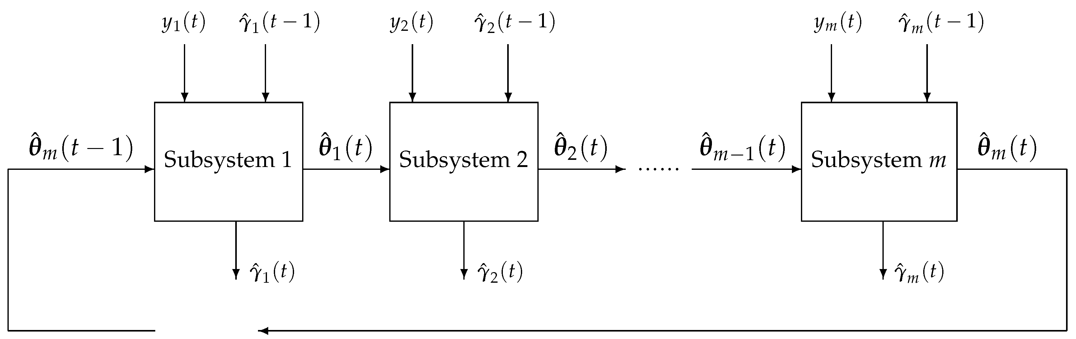
Figure 1.
The schematic diagram of the M-PC-GSG algorithm.

Figure 2.
The M-PC-MI-GSG estimation errors versus t.

Figure 3.
Parameter estimates , , , versus t.

Figure 4.
Parameter estimates , , , versus t.

Figure 5.
The M-PC-MI-GSG estimation errors versus t.

Figure 6.
The true output, the predicted output of and the prediction error.

Figure 7.
The true output, the predicted output of and the prediction error.

Figure 8.
The comparison of algorithms M-FF-GSG with M-PC-MI-GSG.


Table 1.
Parameter estimates and errors ().
| Algorithms | t | 100 | 200 | 500 | 1000 | 2000 | 3000 | True Values |
|---|---|---|---|---|---|---|---|---|
| M-PC-GSG | 0.19022 | 0.28281 | 0.33788 | 0.36637 | 0.36787 | 0.36879 | 0.42000 | |
| 0.77045 | 0.84529 | 0.88400 | 0.91050 | 0.90956 | 0.90832 | 0.93000 | ||
| 0.42624 | 0.49137 | 0.54550 | 0.57360 | 0.57695 | 0.57314 | 0.56000 | ||
| 0.25045 | 0.25999 | 0.29032 | 0.31802 | 0.32379 | 0.32917 | 0.31000 | ||
| −0.16279 | −0.13896 | −0.12959 | −0.13205 | −0.13608 | −0.13540 | −0.25000 | ||
| −0.06264 | 0.01024 | 0.07393 | 0.10879 | 0.14383 | 0.16385 | 0.68000 | ||
| −0.18783 | −0.21131 | −0.22760 | −0.22982 | −0.23502 | −0.23697 | −0.33000 | ||
| 0.06255 | 0.05905 | 0.07305 | 0.09172 | 0.10850 | 0.12021 | 0.44000 | ||
| 60.04604 | 53.54881 | 48.52141 | 45.66110 | 43.08714 | 41.59002 | |||
| M-PC-MI-GSG | 0.24413 | 0.35242 | 0.38045 | 0.39205 | 0.38805 | 0.38809 | 0.42000 | |
| 0.80411 | 0.89433 | 0.91071 | 0.92629 | 0.92058 | 0.91797 | 0.93000 | ||
| 0.49437 | 0.54833 | 0.57802 | 0.58115 | 0.58224 | 0.57102 | 0.56000 | ||
| 0.30721 | 0.28679 | 0.29391 | 0.32301 | 0.32347 | 0.32964 | 0.31000 | ||
| −0.05715 | −0.06016 | −0.08608 | −0.10747 | −0.13040 | −0.13492 | −0.25000 | ||
| 0.12099 | 0.22052 | 0.30492 | 0.34234 | 0.38260 | 0.40361 | 0.68000 | ||
| −0.23138 | −0.26019 | −0.26756 | −0.26447 | −0.26951 | −0.27084 | −0.33000 | ||
| 0.11762 | 0.11798 | 0.15107 | 0.18454 | 0.20984 | 0.22701 | 0.44000 | ||
| 47.51695 | 39.87369 | 33.61530 | 30.01753 | 26.59647 | 24.80351 | |||
| M-PC-MI-GSG | 0.26824 | 0.39655 | 0.39206 | 0.40527 | 0.40117 | 0.40344 | 0.42000 | |
| 0.81764 | 0.91822 | 0.91009 | 0.93027 | 0.92223 | 0.92506 | 0.93000 | ||
| 0.53011 | 0.56224 | 0.57291 | 0.58006 | 0.58163 | 0.56221 | 0.56000 | ||
| 0.33781 | 0.28934 | 0.27962 | 0.32670 | 0.31900 | 0.33021 | 0.31000 | ||
| −0.02859 | −0.07525 | −0.14398 | −0.17985 | −0.21158 | −0.20979 | −0.25000 | ||
| 0.40063 | 0.49444 | 0.57042 | 0.57794 | 0.60699 | 0.61726 | 0.68000 | ||
| −0.27689 | −0.30473 | −0.29946 | −0.29170 | −0.29725 | −0.29909 | −0.33000 | ||
| 0.22503 | 0.21310 | 0.25734 | 0.29682 | 0.32439 | 0.34271 | 0.44000 | ||
| 30.60589 | 22.77807 | 16.20218 | 12.94875 | 9.87303 | 8.55799 | |||
| M-PC-MI-GSG | 0.22875 | 0.41123 | 0.39312 | 0.41067 | 0.40847 | 0.41377 | 0.42000 | |
| 0.82538 | 0.91675 | 0.89962 | 0.92660 | 0.91916 | 0.93461 | 0.93000 | ||
| 0.50062 | 0.56129 | 0.56967 | 0.58480 | 0.57905 | 0.55554 | 0.56000 | ||
| 0.34784 | 0.29455 | 0.27015 | 0.32493 | 0.31639 | 0.33324 | 0.31000 | ||
| −0.08032 | −0.14448 | −0.22262 | −0.25289 | −0.27162 | −0.25101 | −0.25000 | ||
| 0.60874 | 0.66577 | 0.71758 | 0.67480 | 0.69550 | 0.69273 | 0.68000 | ||
| −0.31148 | −0.33276 | −0.30958 | −0.29949 | −0.30552 | −0.31357 | −0.33000 | ||
| 0.32292 | 0.26569 | 0.31977 | 0.36227 | 0.39067 | 0.40749 | 0.44000 | ||
| 20.99172 | 13.61264 | 9.45336 | 5.90521 | 4.39162 | 3.04341 |
Table 2.
Parameter estimates and errors ().
| Algorithms | t | 100 | 200 | 500 | 1000 | 2000 | 3000 | True Values |
|---|---|---|---|---|---|---|---|---|
| M-PC-GSG | −0.38109 | −0.34290 | −0.35197 | −0.35358 | −0.35240 | −0.35140 | −0.36000 | |
| 0.17154 | 0.19202 | 0.22318 | 0.20571 | 0.20894 | 0.20290 | 0.22000 | ||
| 0.52049 | 0.46240 | 0.42063 | 0.40418 | 0.38885 | 0.38130 | 0.34000 | ||
| 0.36772 | 0.39041 | 0.40431 | 0.43059 | 0.44228 | 0.45084 | 0.45000 | ||
| 0.32582 | 0.28799 | 0.27265 | 0.25708 | 0.26433 | 0.26468 | 0.25000 | ||
| −0.05956 | −0.02720 | −0.02478 | −0.02008 | −0.00934 | −0.00876 | 0.11000 | ||
| −0.32562 | −0.33413 | −0.35093 | −0.36678 | −0.37198 | −0.37339 | −0.41000 | ||
| −0.42387 | −0.42801 | −0.43950 | −0.44549 | −0.45522 | −0.45784 | −0.48000 | ||
| −0.07449 | −0.04447 | 0.00357 | 0.05541 | 0.08891 | 0.10599 | 0.35000 | ||
| 0.13315 | 0.09440 | 0.04896 | 0.00007 | −0.03206 | −0.04982 | −0.31000 | ||
| 62.46630 | 55.62215 | 48.66825 | 41.81593 | 37.21977 | 34.99402 | |||
| M-PC-MI-GSG | −0.34351 | −0.30662 | −0.36709 | −0.35952 | −0.35025 | −0.35053 | −0.36000 | |
| 0.13616 | 0.21845 | 0.24620 | 0.20140 | 0.21882 | 0.20575 | 0.22000 | ||
| 0.46447 | 0.34810 | 0.32286 | 0.33605 | 0.34131 | 0.33736 | 0.34000 | ||
| 0.53467 | 0.51841 | 0.49198 | 0.50896 | 0.49490 | 0.49143 | 0.45000 | ||
| 0.34052 | 0.24404 | 0.24150 | 0.23199 | 0.26443 | 0.26536 | 0.25000 | ||
| −0.08458 | −0.00717 | −0.00412 | 0.01422 | 0.05155 | 0.05032 | 0.11000 | ||
| −0.40747 | −0.39750 | −0.42113 | −0.42870 | −0.41996 | −0.41446 | −0.41000 | ||
| −0.44953 | −0.45067 | −0.47122 | −0.47509 | −0.49160 | −0.49275 | −0.48000 | ||
| −0.00019 | 0.05273 | 0.13849 | 0.22633 | 0.25865 | 0.27774 | 0.35000 | ||
| −0.10619 | −0.14079 | −0.18170 | −0.23788 | −0.25384 | −0.26009 | −0.31000 | ||
| 45.05598 | 34.25524 | 25.50852 | 16.96953 | 12.12756 | 10.74341 | |||
| M-PC-MI-GSG | −0.35745 | −0.30970 | −0.38425 | −0.36288 | −0.34050 | −0.34946 | −0.36000 | |
| 0.12136 | 0.23250 | 0.25401 | 0.20572 | 0.22745 | 0.20850 | 0.22000 | ||
| 0.40415 | 0.28647 | 0.30611 | 0.33618 | 0.34589 | 0.33781 | 0.34000 | ||
| 0.51978 | 0.48285 | 0.46617 | 0.48824 | 0.46462 | 0.46024 | 0.45000 | ||
| 0.38782 | 0.22572 | 0.22904 | 0.22473 | 0.27031 | 0.26832 | 0.25000 | ||
| −0.02008 | 0.06621 | 0.05334 | 0.06901 | 0.10837 | 0.09507 | 0.11000 | ||
| −0.41690 | −0.39157 | −0.43170 | −0.43710 | −0.42419 | −0.41720 | −0.41000 | ||
| −0.46440 | −0.45497 | −0.48430 | −0.48122 | −0.50181 | −0.49994 | −0.48000 | ||
| 0.09086 | 0.14050 | 0.23086 | 0.31994 | 0.33401 | 0.34857 | 0.35000 | ||
| −0.24541 | −0.23841 | −0.25163 | −0.30483 | −0.29672 | −0.29278 | −0.31000 | ||
| 32.60246 | 22.30989 | 14.47746 | 6.91170 | 4.31185 | 3.73785 |
Publisher’s Note: MDPI stays neutral with regard to jurisdictional claims in published maps and institutional affiliations. |
© 2022 by the authors. Licensee MDPI, Basel, Switzerland. This article is an open access article distributed under the terms and conditions of the Creative Commons Attribution (CC BY) license (https://creativecommons.org/licenses/by/4.0/).
Share and Cite
MDPI and ACS Style
Ma, P.; Wang, L. Partially Coupled Stochastic Gradient Estimation for Multivariate Equation-Error Systems. Mathematics 2022, 10, 2955. https://doi.org/10.3390/math10162955
AMA Style
Ma P, Wang L. Partially Coupled Stochastic Gradient Estimation for Multivariate Equation-Error Systems. Mathematics. 2022; 10(16):2955. https://doi.org/10.3390/math10162955
Chicago/Turabian StyleMa, Ping, and Lei Wang. 2022. "Partially Coupled Stochastic Gradient Estimation for Multivariate Equation-Error Systems" Mathematics 10, no. 16: 2955. https://doi.org/10.3390/math10162955
Note that from the first issue of 2016, this journal uses article numbers instead of page numbers. See further details here.