Investigation of Exact Solutions of Nonlinear Evolution Equations Using Unified Method

Abstract

In this article, an analytical technique based on unified method is applied to investigate the exact solutions of non-linear homogeneous evolution partial differential equations. These partial differential equations are reduced to ordinary differential equations using different traveling wave transformations, and exact solutions in rational and polynomial forms are obtained. The obtained solutions are presented in the form of 2D and 3D graphics to study the behavior of the analytical solution by setting out the values of suitable parameters. The acquired results reveal that the unified method is a suitable approach for handling non-linear homogeneous evolution equations.

1. Introduction

Nonlinear homogeneous evolution equations form the most fundamental theme in mathematical physics. In a few decades, due to its wide application, nonlinear evolution equations have become a very significant class of PDEs. The investigation of nonlinear evolution equations has become a very important topic in major fields such as plasma physics, solid state physics, fluid mechanics, biology, optical fiber, chemical kinematics, economics and many more [1,2,3,4,5,6]. A few years ago, various types of well-known mathematical methods were used to solve the nonlinear homogeneous PDEs for obtaining exact solutions, such as the tanh method [7], Exp-function method [8,9], $\left(\frac{G^{\prime }}{G}\right)$-expansion method [10,11,12,13,14], projective Riccati equation method [15], bilinear transformation method [16,17,18,19,20], higher degree B-spline algorithm [21], spectral Tau method [22], Adomian decomposition and fractional power series solution [23] and some higher–degree Lacunary fractional splines [24]. Therefore, it is not an easy task to use analytical methods for solving nonlinear PDEs [25].

Many of researchers investigate different homogeneous nonlinear PDEs for constructing traveling wave solution by applying the unified method (UM). For example, MN Rafique [26] used the unified method to find exact solutions of fifth-order Swada–Kotera and Caudrey–Dodd–Gibbon equations. In [27], UM was applied to establish a traveling wave solution of the higher-dimensional Chaffee–Infante equation. Majeed et al. [28] constructed traveling wave solutions for a modified Burgers-KdV equation using the unified method.

In [29], an analytical solution of the advection–diffusion reaction equation, which represents the exponential traveling wave in heat and mass transport processes, was compared to the unconditionally positive finite difference (UPFD) and standard explicit finite difference methods. Although the UPFD scheme has unconditional positivity, it is found that it is less accurate than the standard explicit finite difference scheme.

The key objective of this study is to find the exact solution of the generalized regularized long wave (GRLW) equation [30] and the modified Zakharov–Kuznetsov (mZK) equation [31]. For this purpose, we use different traveling wave transformations to convert the homogeneous nonlinear partial differential equation (PDE) into the nonlinear ordinary differential equation (ODE) [32]. To find the variety of new exact solutions, the UM is proposed [33].

In this work, we discuss two nonlinear homogeneous evolution PDEs. The first one is the generalized regularized long wave (GRLW) equation of the following form [30]:

$$u_t+u_x+\alpha u^P{u}_x-\mu u_{xxt}=0,(x,t)ϵ\mathbb{R}\times \left[0T\right].$$

(1)

In Equation (1), the value of parameter P is a natural number and α, μ are positive constants. When the value of parameter P = 1, Equation (1) becomes a regularized long wave (RLW) equation. Equation (1) becomes a modified regularized long wave MRLW equation for P = 2.

The modified Zakharov–Kuznetsov (mZK) equation is of the form [34]

$$m_t+\beta m^2{m}_x+m_{xxx}+m_{yyx}=0.$$

(2)

The nonlinear Equation (2) consist of two spatial, x and y, and one temporal coordinate. Equation (2) explains the properties of weakly nonlinear ion sound waves in plasma. This includes the cold and hot isothermal electrons in the presence of a uniform magnetic field. In previous literature, many researchers studied the mZK equation by using different methods. For instance, in [35], the homogeneous balance method was used to investigate the exact solutions of the mZK equation. Bekir [36] used the basic $(G^{\prime }/G)$-expansion method to construct traveling wave solutions of the mZK equation.

In the study of nonlinear physical phenomena, the investigation of traveling wave solutions of nonlinear homogeneous partial differential equations plays an important role [37]. We obtain these solutions as two different types, namely, polynomial solution and rational solution. The 2D and 3D diagrams of these solutions are plotted with specific values for their existing parameters. The behavior of the solution of these governing equations will be revealed by examining these graphs. Maple software is used for simulations. The proposed techniques can be used in other real-world models in engineering and science. The unified method is used to investigate non-linear evolution equations that prove the importance of these equations. The main objectives of this study are listed below:

• To analyze the unified method;
• To find exact solutions of different nonlinear homogeneous partial differential equations (PDEs) using the unified method;
• To obtain analytical solutions in polynomial as well as rational forms;
• To represent their nonlinear physical behavior through 2D and 3D graphics.

The rest of the study demonstrated in the following manner: Section 2 presents the description of the unified method. In Section 3, a new exact solution of the generalized regularized long wave equation and modified Zakharov–Kuznetsov equation and their graphical representation in 2D and 3D forms is presented. In Section 4, we describe the advantages and limitations of this proposed scheme. In Section 5, we discuss the graphical behavior. Finally, we present a brief conclusion in Section 6.

2. Description of Unified Method

Let us discuss the general form of non-linear PDE for $w(x,y,t)$ in the form of

$$\begin{array}{c}\hfill S(x,y,t,w,\frac{\partial w}{\partial x},\frac{\partial w}{\partial y},\frac{\partial w}{\partial t},\frac{{\partial }^{2}w}{\partial x\partial t},\frac{{\partial }^{2}w}{\partial x^2},\cdots )=0.\end{array}$$

(3)

where S is a function of the polynomial, and the subscripts represent the partial derivative with respect to variables $x,y,t$. The unified method for solving evolution nonlinear PDEs is defined in the following steps.

Step 1. Change the given PDE into ODE using traveling wave transformation $\eta =x+y-vt$, to Equation (3).

So this results in an ODE with the following structure:

$$\begin{array}{c}\hfill S(w,\frac{dw}{d\eta },\frac{d^{2}w}{d{\eta }^2},\dots )=0.\end{array}$$

(4)

Step 2. In this step, we find the polynomial and rational solutions of Equation (4).

2.1. Polynomial Solution

To obtain the polynomial solution of nonlinear PDEs, we assume that,

$$\begin{array}{cc}\hfill w\left(\eta \right)& =\sum _{i=0}^{\mathit{N}}{a}_i{\varphi }^{i\left(\eta \right)},\hfill \\ \hfill {\left({\varphi }^{\prime }\left(\eta \right)\right)}^{\rho }& =\sum _{i=0}^{\rho s}{b}_i{\varphi }^i\left(\eta \right),\hfill & \rho =1,2.\end{array}$$

(5)

where $a_i,b_i$ are the unknown coefficients of the polynomial which are obtained from Equation (5) to satisfy Equation (4) by applying the condition of consistency. Now, N and s are the parameters which are determined with the help of the homogeneous balancing principle by comparing the highest order linear derivative along with the nonlinear term.

It should be noted that the unified method solves Equation (5) for $\rho =1$ or $\rho =2$ for elementary or elliptical solutions, respectively.

2.2. Rational Solution

To obtain these solutions, we assume that

$$\begin{array}{cc}\hfill w\left(\eta \right)& =\frac{{\sum }_{i=0}^n{a}_i{\varphi }^i\left(\eta \right)}{{\sum }_{i=0}^r{c}_i{\varphi }^i\left(\eta \right)},\hfill \\ \hfill {\left({\varphi }^{\prime }\left(\eta \right)\right)}^{\rho }& =\sum _{i=0}^{\rho s}{b}_i{\varphi }^i\left(\eta \right),\hfill & \rho =1,2.\end{array}$$

(6)

where $a_i$, $b_i$ are unknown coefficients of Equation (6) which are to be determined in such a way that the obtained solution from Equation (6) must satisfy Equation (4). These unknown coefficients that appear in Equation (6) are determined through the condition of consistency. Now, n, r and s are parameters which are determined with the help of the balancing principle by comparing the highest order linear derivative along with the nonlinear terms.

It should be noted that the unified method solves Equation (6) for $\rho =1$ or $\rho =2$ for elementary or elliptical solutions, respectively.

Step 3. Computer software, such as Maple or Mathematica, are used to solve the system of equations.

Step 4. In this step, we solve Equations (5) and (6) and obtain an analytical solution.

3. Governing Equation

We discuss two nonlinear homogeneous PDEs, namely, the generalized regularized long wave equation (GRLWE), Equation (1), and modified Zakharov–Kuznetsov (mZK) equation, Equation (2).

3.1. Generalized Regularized Long Wave Equation (GRLWE)

In this section, we discuss the generalized regularized long wave equation for P = 1, P = 2.

Let us consider GRLWE [34],

$$u_t+u_x+\alpha u^P{u}_x-\mu u_{xxt}=0.$$

(7)

In Equation (7), P represents a positive integer. α and μ are positive constants. According to these parameters, we divide Equation (7) into two types.

• Regularized long wave (RLW) equation for P = 1.
• Modified regularized long wave (MRLW) equation for P = 2.

3.1.1. Regularized Long Wave Equation for P = 1

Equation (7) becomes

$$u_t+u_x+\alpha u{u}_x-\mu u_{xxt}=0.$$

(8)

In order to solve Equation (8) using the unified method, apply traveling wave transformation in the following form.

$$u\left(x,t\right)=u\left(\eta \right),\eta =x-vt.$$

(9)

After applying the transformation, we draw out ODE of the form

$$-v{u}^{\prime }+u^{\prime }+\alpha u{u}^{\prime }+\mu v{u}^{‴}=0.$$

(10)

In Equation (10), prime (′) shows the derivative with respect to η.

For simplicity, we integrate the above ODE and fix the integration constant equal to zero,

$$-vu+u+\frac{1}{2}\alpha u^2+\mu v{u}^{″}=0.$$

(11)

We obtain solutions of Equation (11) using the unified method which enables us to find those solutions in two ways, namely, the polynomial function solution as well as rational function solution.

Polynomial Function Solution

Suppose the initial solution is given by

$$\begin{array}{cc}\hfill u\left(\eta \right)& =\sum _{i=0}^N{a}_i{\varphi }^{i\left(\eta \right)},\hfill \\ \hfill {\left({\varphi }^{\prime }\left(\eta \right)\right)}^{\rho }& =\sum _{i=0}^{\rho s}{b}_i{\varphi }^i\left(\eta \right),\hfill & \rho =1,2.\end{array}$$

(12)

$a_i$ and $b_i$ are unknown coefficients of Equation (12) which can be find later.

Now, using the homogeneous balancing principle between dispersive and nonlinear term, we obtain the integer N2. After applying the balancing principle, we establish a relation between N and s, such as N = s− 1 for all s ≥ 2. After integrating Equation (10), the balancing number will be same as that of Equation (11).

For the polynomial function solution, we discuss two cases for $s=2, \rho =1$ and $s=2, \rho =2$. Equation (12) becomes

$$u\left(\eta \right)=\sum _{i=0}^2{a}_i{\varphi }^{i\left(\eta \right)}.$$

(13)

$${\left({\varphi }^{\prime }\left(\eta \right)\right)}^{\rho }=\sum _{i=0}^{2\rho }{b}_i{\varphi }^i\left(\eta \right),\rho =1,2.$$

(14)

Here $a_i$, $b_i$ are coefficients which can be found later.

• Case (1)

Here we put $\rho =1$ and $s=2$ in Equations (14) and (13), and Equation (14) becomes,

$$\begin{array}{c}\hfill u\left(\eta \right)=a_0+a_1\varphi \left(\eta \right)+a_2{\varphi }^2\left(\eta \right),\\ \hfill {\varphi }^{\prime }\left(\eta \right)=b_0+b_1\varphi \left(\eta \right)+b_2{\varphi }^2\left(\eta \right),\end{array}$$

(15)

Substitute Equation (15) into Equation (11) and solve the system of algebraic equations in ϕ using computer software for ($b_0,b_1,b_2,a_0,a_1,a_2,v,\mu ,\alpha$). We obtain the following results:

$$\alpha =\frac{-12\beta v{b}_2^2}{a_2},a_0=\frac{3\beta v{a}_1^2{b}_2^2+v{a}_2^2-a_2^2}{12\beta v{a}_2{b}_2^2},b_0=\frac{\beta v{a}_1^2{b}_2^2+v{a}_2^2-a_2^2}{4\beta v{a}_2^2{b}_2},b_1=\frac{a_1{b}_2}{a_2}.$$

(16)

and putting Equation (15) in Equation (16), as a consequence, the following result is obtained.

$$u(x,t)=-\frac{(v-1)(a_2{b}_{2}tan{\left(\frac{1}{2}\eta \sqrt{-\frac{b_2(v-1)}{\beta v{b}_2}}\right)}^2+a_2{b}_2)}{4b_2\beta b_2^2}.$$

(17)

where $\eta =x-vt$ and $\beta \ne 0$, $v\ne 0$, $b_2\ne 0$.

Graphically, Equation (17) is shown in Figure 1 with suitable parameters a₂ = 4, b₂ = 1.4, v = 2, β = 1.2.

Figure 1 illustrates dynamics of soliton solutions in 2D and 3D graphs obtained in Equation (17). Figure 1a,b plots the graphs at different values of parameters (a₂ = 4, b₂ = 1.4, v = 2, β = 1.2).

• Case (2)

Here we put $\rho =2$ and $s=2$ in Equations (14) and (13), and Equation (14) becomes

$$\begin{array}{cc}\hfill u\left(\eta \right)& =a_0+a_1\varphi \left(\eta \right)+a_2{\varphi }^2\left(\eta \right),\hfill \\ \hfill \left({\varphi }^{\prime }\left(\eta \right)\right)& =\varphi \left(\eta \right)\sqrt{{\beta }_0+{\beta }_1\varphi \left(\eta \right)+{\beta }_2{\left(\varphi \left(\eta \right)\right)}^2}.\hfill \end{array}$$

(18)

Putting Equation (18) into Equation (11) and solving the system of equations in ϕ using computer software for ($a_0$, $a_1$, $a_2$${\beta }_0$, ${\beta }_1$, ${\beta }_2$, v, μ, α), we obtain the following parameters:

$$a_0=0,\alpha =-12\frac{a_2\left(v,-,1\right)}{a_1^2},{\beta }_0=\frac{v-1}{v\beta },{\beta }_1=2\frac{a_2\left(v,-,1\right)}{v{a}_1\beta },{\beta }_2=\frac{a_2^2\left(v,-,1\right)}{v{a}_1^2\beta },$$

(19)

and substituting Equation (19) in Equation (18), as a consequence, the following result is obtained.

$$\begin{array}{c}\hfill u(x,t)=\frac{4(v-1)e^{\eta \sqrt{\frac{v-1}{v\beta }}}{a}_1^{3}v\beta e^{C\sqrt{\frac{v-1}{v\beta }}}}{{\left[-4a_2(v-1)e^{C\sqrt{\frac{v-1}{v\beta }}}+e^{\eta \sqrt{\frac{v-1}{v\beta }}}{a}_{1}v\beta \right]}^2}.\end{array}$$

(20)

where C is a constant and $\eta =x-vt$ and $v\ne 0$, $\beta \ne 0$.

Graphically, Equation (20) is shown in Figure 2 with suitable parameters a₁ = − 0.3, a₂ = 2.4, v = 3, β = 2, C = 0.

Figure 2 illustrates optical soliton solutions in 2D and 3D graphs obtained in Equation (20). Figure 2a,b plots the graphs at different values of parameters (a₁ = − 0.3, (a₂ = 2.4, v = 3, β = 2, C = 0).

Rational Function Solution

Suppose the initial solution in the following form,

$$u(x,t)=\frac{{\sum }_{i=0}^n{a}_i{\varphi }^i\left(\eta \right)}{{\sum }_{i=0}^r{c}_i{\varphi }^i\left(\eta \right)},$$

(21)

$${\left({\varphi }^{\prime }\left(\eta \right)\right)}^{\rho }=\sum _{i=0}^{\rho s}{b}_i{\varphi }^i\left(\eta \right),\rho =1,2.$$

(22)

where $a_i$, $b_i$, $c_i$ are unknown coefficients which are to be determined later. After using the homogeneous balancing principle, we obtain the relation that states that $n-r=s-1$.

Here, we discuss only one case when $n=r$ and $\rho =2$. So Equations (21) and (22) give

$$u(x,t)=\frac{a_0+a_1\varphi \left(\eta \right)+a_2{\varphi }^2\left(\eta \right)}{c_0+c_1\varphi \left(\eta \right)+c_2{\varphi }^2\left(\eta \right)}.$$

(23)

$$\left({\varphi }^{\prime }\left(\eta \right)\right)=\sqrt{b_0+b_1\varphi \left(\eta \right)+b_2{\varphi }^2\left(\eta \right)}.$$

(24)

Putting Equations (23) and (24) into Equation (11) and solving the system of equations in ϕ using computer software for (a₀, a₁, a₂, c₀, c₁, c₂, b₀, b₁, b₂, v, μ, α), we obtain the following parameters:

$$\begin{array}{c}\hfill \alpha =2\frac{c_2\left(v,-,1\right)}{a_2},a_0=-1/8\frac{a_2\left(4,,c_0,c_2,-,3,,c_1^2\right)}{c_2^2},a_1=\frac{a_2{c}_1}{c_2},\\ \hfill b_0=-1/4\frac{c_0\left(v-1\right)}{v\beta c_2},b_1=-1/4\frac{c_1\left(v-1\right)}{v\beta c_2},b_2=-1/4\frac{v-1}{v\beta },\end{array}$$

(25)

and putting Equation (25) in Equations (23) and (24), as a consequence, the following solution is obtained.

$$u(x,t)=\frac{a_2[16(c_0{c}_2-\frac{1}{4}{c}_1^2)\beta v{c}_2^2(v-1)e^{\sqrt{\frac{-v+1}{v\beta }}(C+\eta )}+{(c_0{c}_2-\frac{1}{4}{c}_1^2)}^2{(v-1)}^2{e}^{2C\sqrt{\frac{-v+1}{v\beta }}}+16e^{2\eta \sqrt{\frac{-v+1}{v\beta }}}{v}^2{\beta }^2{c}_2^4]}{c_2[-8(c_0{c}_2-\frac{1}{4}{c}_1^2)\beta v{c}_2^2(v-1)e^{\sqrt{\frac{-v+1}{v\beta }}(C+\eta )}+{(c_0{c}_2-\frac{1}{4}{c}_1^2)}^2{(v-1)}^2{e}^{2C\sqrt{\frac{-v+1}{v\beta }}}+16e^{2\eta \sqrt{\frac{-v+1}{v\beta }}}{v}^2{\beta }^2{c}_2^4]}.$$

(26)

where $\eta =x-vt$ and C is constant of integration and $v\ne 0$, $\beta \ne 0$.

Figure 3 shows a graphical representation of Equation (26) with suitable parameters $c_0=1.3,c_1=2,c_2=3,a_2=1,v=-5,\beta =-1,C=0$.

3.1.2. Modified Regularized Long Wave Equation for P = 2

Equation (7) becomes,

$$u_t+u_x+ϵu^2{u}_x-\mu u_{xxt}=0.$$

(27)

In order to solve Equation (27) using the unified method, apply transformation in the following way:

$$u\left(x,t\right)=u\left(\eta \right),\eta =x-vt.$$

(28)

After applying these transformation, we draw out ODE of the form

$$-v{u}^{\prime }+u^{\prime }+ϵu^2{u}^{\prime }+\mu v{u}^{‴}=0.$$

(29)

In Equation (29), prime (′) shows the derivative with respect to η.

For simplicity, we integrate the above ODE and fix the integration constant equal to zero.

$$-vu+u+\frac{1}{3}ϵu^3+\mu v{u}^{\prime \prime }=0.$$

(30)

We obtain solutions of Equation (30) using the unified method that enable to find these solutions in two kinds, namely, the polynomial function solution and rational function solution.

Polynomial Function Solution

Suppose the initial solution is given by

$$\begin{array}{cc}\hfill u\left(\eta \right)& =\sum _{i=0}^N{a}_i{\varphi }^{i\left(\eta \right)},\hfill \\ \hfill {\left({\varphi }^{\prime }\left(\eta \right)\right)}^{\rho }& =\sum _{i=0}^{\rho s}{b}_i{\varphi }^i\left(\eta \right),\rho =1,2.\hfill \end{array}$$

(31)

where $a_i$ and $b_i$ are coefficients of the polynomial, which can be found later.

Now, considering the homogeneous balancing principle between the nonlinear and dispersive term, we obtain the value of integer $N=1$, after which results a relation $N=s-1$ for all $k\ge 2$.

For the polynomial function solution, $s=2,\rho =1$ and $s=2,\rho =2$, are two different cases, which we will discuss. The above equation can be converted into,

$$u\left(\eta \right)=\sum _{i=0}^1{a}_i{\varphi }^{i\left(\eta \right)}.$$

(32)

$${\left({\varphi }^{\prime }\left(\eta \right)\right)}^{\rho }=\sum _{i=0}^{2\rho }{b}_i{\varphi }^i\left(\eta \right),\rho =1,2.$$

(33)

Here, $a_i$, $b_i$ are coefficients which can be found later.

• Case (1)

Here, we put $\rho =1$ and $s=2$ in Equation (33), and after this, Equations (32) and (33) become,

$$\begin{array}{cc}\hfill u(x,t)& =a_0+a_1\varphi \left(\eta \right),\hfill \\ \hfill {\varphi }^{\prime }\left(\eta \right)& =b_0+b_1\varphi \left(\eta \right)+b_2{\varphi }^2\left(\eta \right).\hfill \end{array}$$

(34)

Substitute Equation (34) into Equation (30), and solving the system of equations in ϕ using computer software for $a_0,a_1,b_0,b_1,b_2,v,\mu ,\alpha$, we obtain the following parameters:

$$\alpha =-6\frac{v\beta b_2^2}{a_1^2},b_0=1/2\frac{2v{a}_0^2\beta b_2^2+v{a}_1^2-a_1^2}{v{a}_1^2\beta b_2},b_1=2\frac{a_0{b}_2}{a_1},$$

(35)

and inserting Equations (35) in (34), we obtain the following result:

$$u(x,t)=\frac{tan\left[\frac{1}{2}\eta \sqrt{\frac{2b_2(v-1)}{v\beta b_2}}\right]a_1\sqrt{\frac{2b_2(v-1)}{v\beta b_2}}}{2b_2}.$$

(36)

where $\eta =x-vt$ and $\beta \ne 0$, $v\ne 0$, $b_2\ne 0$.

Figure 4 shows the graphical behavior of Equation (36) with suitable parameters $a_0=-1.3,$$a_1=2.3,b_2=1.9,v=0.4,\beta =2.$

• Case (2)

Here, we put $s=2$ and $\rho =2$ in Equation (33) and after this, Equations (32) and (33) become

$$\begin{array}{cc}\hfill u\left(\eta \right)& =a_0+a_1\varphi \left(\eta \right)+a_2{\varphi }^2\left(\eta \right),\hfill \\ \hfill \left({\varphi }^{\prime }\left(\eta \right)\right)& =\varphi \left(\eta \right)\sqrt{{\beta }_0+{\beta }_1\varphi \left(\eta \right)+{\beta }_2\left({\varphi }^2,\left(\eta \right)\right)}.\hfill \end{array}$$

(37)

putting Equation (37) into Equation (30) and solving system of algebraic equations in $\varphi$ using computer software for $a_0$, $a_1$, ${\beta }_0$, ${\beta }_1$, ${\beta }_2$, v, $\mu$, $\alpha$, we obtain the following parameters:

$$\alpha =\frac{3(v-1)}{a_0^2},{\beta }_0=-\frac{2(v-1)}{\beta v},{\beta }_1=-\frac{2a_1(v-1)}{a_0\beta a_0^2},b_2=-\frac{a_1^2(v-1)}{2\beta v{a}_0^2},$$

(38)

and substituting Equation (38) in Equation (37), we obtain the following result.

$$u(x,t)=-\frac{4[a_1(v-1)e^{\eta \sqrt{\frac{-2v+2}{v\beta }}}-\frac{1}{4}{e}^{C\sqrt{\frac{-2v+2}{v\beta }}}{a}_0\beta ]a_0}{4a_1(v-1)e^{\eta \sqrt{\frac{-2v+2}{v\beta }}}+e^{C\sqrt{\frac{-2v+2}{v\beta }}}{a}_0\beta v}.$$

(39)

where C is constant of integration and $\eta =x-vt$, $v\ne 0$, $\beta \ne 0$.

Graphical behavior of Equation (39) as shown in Figure 5 with suitable parameters $a_0=-1,a_1=2.6,v=2,\beta =-2,C=1$.

Rational Functional Solutions

Suppose the initial solution is in the following form:

$$u(x,t)=\frac{{\sum }_{i=0}^n{a}_i{\varphi }^i\left(\eta \right)}{{\sum }_{i=0}^r{c}_i{\varphi }^i\left(\eta \right)}.$$

(40)

$${\left({\varphi }^{\prime }\left(\eta \right)\right)}^{\rho }=\sum _{i=0}^{\rho s}{b}_i{\varphi }^i\left(\eta \right),\rho =1,2.$$

(41)

where $a_i,b_i,c_i$ are unknown coefficients which are to be determined later. After using the homogeneous balancing principle, we obtain the relation that states that $n-r=s-1$.

Here we discuss only one case when $n=r$ and $\rho =2$. Equations (40) and (41) gives,

$$\begin{array}{cc}\hfill u(x,t)& =\frac{a_0+a_1\varphi \left(\eta \right)}{c_0+c_1\varphi \left(\eta \right)},\hfill \\ \hfill \left({\varphi }^{\prime }\left(\eta \right)\right)& =\sqrt{b_0+b_1\varphi \left(\eta \right)+b_2{\left(\varphi \left(\eta \right)\right)}^2}.\hfill \end{array}$$

(42)

Putting Equation (42) into Equation (30) and solving the system of equations in $\varphi$ using Maple software for ($a_0,a_1,c_0,c_1,b_0,b_1,b_2,v,\mu ,\alpha$), we obtain the following parameters:

$$\begin{array}{cc}\hfill \alpha & =\frac{3c_1^2(v-1)}{a_1^2},b_0=-\frac{v{a}_0^2{c}_1^2+2v{a}_0{a}_1{c}_0{c}_1+v{a}_1^2{c}_0^2-a_0^2{c}_1^2-2a_0{a}_1{c}_0{c}_1-a_1^2{c}_0^2}{v\beta a_1^2{c}_1^2},\hfill \\ \hfill b_1& =-\frac{2(v{a}_0{c}_1+v{a}_1{c}_0-a_0{c}_1-a_1{c}_0)}{v\beta a_1{c}_1},b_2=-\frac{2(v-1)}{v\beta },\hfill \end{array}$$

(43)

and inserting Equation (43) in Equation (42), we obtain the following result.

$$u(x,t)=\frac{a_1[e^{\eta \sqrt{\frac{-2v+2}{v\beta }}}{a}_1{c}_1+\sqrt{\frac{-2v+2}{v\beta }}{e}^{C\sqrt{\frac{-2v+2}{v\beta }}}(a_0{c}_1-a_1{c}_0)]}{c_1[e^{\eta )\sqrt{\frac{-2v+2}{v\beta }}}{a}_1{c}_1-\sqrt{\frac{-2v+2}{v\beta }}{e}^{C\sqrt{\frac{-2v+2}{v\beta }}}(a_0{c}_1-a_1{c}_0)]}.$$

(44)

where C is a constant of integration and $\eta =x-vt$ and $v\ne 0$, $\beta \ne 0$, $b_2\ne 0$.

The graphical behavior of Equation (44) is shown in Figure 6 with suitable parameters $a_0=1.9,a_1=2.3,c_0=2.8,c_1=2.8,v=1.3,\beta =-1.2,C=0.$

3.2. Modified Zakharov–Kuznetsov Equation (mZK)

Here, we find the exact solution of the modified ZK equation using the unified method. So, the nonlinear mZK equation [35],

$$m_t+\beta m^2{m}_x+m_{xxx}+m_{yyx}=0.$$

(45)

where $\beta$ is a positive constant.

In order to solve Equation (45) using the unified method, apply transformation in the following way.

$$m(x,y,t)=m\left(\eta \right),\eta =x+y-vt.$$

(46)

After applying transformation, we draw out ODE of this form,

$$-v{m}^{\prime }+\beta m^2{m}^{\prime }+2m^{‴}=0.$$

(47)

In Equation (47), prime (′) shows derivative w.r.t $\eta$,

For simplicity, integrate the above Equation (47) and fix the integration constant equal to zero,

$$-3vm+\beta m^3+6m^{″}=0.$$

(48)

We obtain solutions of Equation (48) using the unified method that enables us to find those solutions in two kinds, namely, the polynomial function solution as well as the rational function solution.

3.2.1. Polynomial Function Solution

Suppose the auxiliary equation is in the following form,

$$\begin{array}{cc}\hfill m\left(\eta \right)& =\sum _{i=0}^{\mathit{N}}{a}_i{\varphi }^{i\left(\eta \right)},\hfill \\ \hfill {\left({\varphi }^{\prime }\left(\eta \right)\right)}^{\rho }& =\sum _{i=0}^{\rho p}{b}_i{\varphi }^i\left(\eta \right),\rho =1,2.\hfill \end{array}$$

(49)

where $a_i$ and $b_i$ are coefficients of the polynomial, which can be find later.

Now, using the homogeneous balancing principle between the dispersive and nonlinear terms, we obtain integer $N=1$ after applying the balancing principle to form a relation between N and p, such as $N=p-1$ for all $s\ge 2$.

For polynomial function solutions, $p=2$, $\rho =1$ and $p=2$, $\rho =2$ are two different cases, which we will discuss. The above equation can be converted into

$$m\left(\eta \right)=\sum _{i=0}^1{a}_i{\varphi }^{i\left(\eta \right)}.$$

(50)

$${\left({\varphi }^{\prime }\left(\eta \right)\right)}^{\rho }=\sum _{i=0}^{2\rho }{b}_i{\varphi }^i\left(\eta \right),\rho =1,2.$$

(51)

Here, $a_i$, $b_i$ are coefficients which can be found later.

• Case (1)

Here, we put $\sigma =1$ and $k=2$ in Equation (51), and after this, Equations (50) and (51) become

$$\begin{array}{cc}\hfill m(x,y,t)& =a_0+a_1\left(\eta \right),\hfill \\ \hfill {\varphi }^{\prime }\left(\eta \right)& =b_0+b_1\varphi \left(\eta \right)+b_2{\varphi }^2\left(\eta \right).\hfill \end{array}$$

(52)

Putting Equation (52) into Equation (48) and solving the system of equations in $\varphi$ using computer software for $a_0,a_1,b_0,b_1,b_2,v,\beta$, we obtain the following values of parameters:

$$v=4b_0{b}_2-b_1^2,a_0=\frac{a_1{b}_1}{2b_2},\beta =-\frac{12b_2^2}{a_1^2},$$

(53)

and putting all above values of Equation (53) in Equation (52), we obtain the following result:

$$m(x,y,t)=\frac{a_1(tan\left(\frac{\eta \sqrt{4b_0{b}_2-b_1^2}}{2}\right)\sqrt{4b_0{b}_2-b_1^2}-b_1)}{2b_2}+\frac{a_1{b}_1}{2b_2}.$$

(54)

where $\eta =x+y-vt$ and $b_2\ne 0$.

Figure 7 shows a graphical visualization of Equation (54) with suitable parameters $a_1=2.5,b_0=-0.2,b_1=1.4,b_2=1.8,v=1,y=2.$

• Case (2)

Here, we put $\rho =2$ and $p=2$ in Equation (51) and we obtain the following equations,

$$\begin{array}{cc}\hfill m\left(\eta \right)& =a_0+a_1\varphi \left(\eta \right),\hfill \\ \hfill \left({\varphi }^{\prime }\left(\eta \right)\right)& =\varphi \left(\eta \right)\sqrt{{\beta }_0+{\beta }_1\varphi \left(\eta \right)+{\beta }_2{\varphi }^2\left(\eta \right)}.\hfill \end{array}$$

(55)

Putting Equation (55) into Equation (48) and solving the system of equations in $\varphi$ using computer software for $a_0,a_1,{\beta }_0,{\beta }_1,{\beta }_2,v,\beta$, we obtain the following values of parameters:

$$v=\frac{\beta a_0^2}{3},{\beta }_0=-\frac{\beta a_0^2}{3},{\beta }_1=-\frac{\beta a_0{a}_1}{3},{\beta }_2=-\frac{\beta a_1^2}{12}.$$

(56)

and substituting Equation (56) in Equation (55), we obtain the following solution:

$$m(x,y,t)=-\frac{2(\beta a_0{a}_1{e}^{\eta \sqrt{-\frac{\beta a_0^2}{3}}}-\frac{3}{2}{e}^{C\sqrt{-\frac{\beta a_0^2}{3}}})a_0}{2\beta a_0{a}_1{e}^{\eta \sqrt{-\frac{\beta a_0^2}{3}}}+3e^{C\sqrt{-\frac{\beta a_0^2}{3}}}}.$$

(57)

where C is a constant of integration and $\eta =x+y-vt$.

Graphically, Equation (57) is shown in Figure 8 with suitable parameters $a_0=-2.3,a_1=2.4,y=2,v=1.4,\beta =-1.6,C=0$.

3.2.2. Rational Function Solution

Suppose the initial solution is given by

$$m(x,y,t)=\frac{{\sum }_{i=0}^n{a}_i{\varphi }^i\left(\eta \right)}{{\sum }_{i=0}^r{c}_i{\varphi }^i\left(\eta \right)}.$$

(58)

$${\left({\varphi }^{\prime }\left(\eta \right)\right)}^{\rho }=\sum _{i=0}^{\rho p}{b}_i{\varphi }^i\left(\eta \right),\rho =1,2.$$

(59)

where $a_i,b_i,c_i$ are constants of coefficient which are to be determined later. After using the balancing principle, we obtain the relation that states that $n-r=k-1$.

Here, we discuss only one case when $n=r$ and $\sigma =2$. Equations (58) and (59) give

$$m(x,y,t)=\frac{a_0+a_1\varphi \left(\eta \right)}{c_0+c_1\varphi \left(\eta \right)}.$$

(60)

$${\left({\varphi }^{\prime }\left(\eta \right)\right)}^{\sigma }=\sqrt{b_0+b_1\varphi \left(\eta \right)+b_2{\varphi }^2\left(\eta \right)}.$$

(61)

Putting Equations (60) and (61) into Equation (45) and solving the system of equations in $\varphi$ using computer software for ($a_0,a_1,b_0,b_1,b_2,c_0,c_1,v,\beta$), we obtain the following values of parameters:

$$\beta =\frac{3v{c}_1^2}{a_1^2},b_0=-\frac{v(a_0^2{c}_1^2+2a_0{a}_1{c}_0{c}_1+a_1^2{c}_0^2)}{4a_1^2{c}_1^2},b_1=-\frac{v(a_0{c}_1+a_1{c}_0)}{a_1{c}_1},b_2=-v.$$

(62)

and inserting Equation (62) in Equations (60) and (61), we obtain the following results.

$$m(x,y,t)=\frac{a_1[-e^{\left(\eta \right)\sqrt{-v}}v{a}_1{c}_1+e^{C\sqrt{-v}}(2a_0{c}_1{(-v)}^{\frac{3}{2}}+v(a_0{c}_1+a_1{c}_0)\sqrt{-v})]}{c_1[-e^{\left(\eta \right)\sqrt{-v}}v{a}_1{c}_1+e^{C\sqrt{-v}}(2a_0{c}_1{(-v)}^{\frac{3}{2}}+v(a_0{c}_1+a_1{c}_0)\sqrt{-v})]}.$$

(63)

where $\eta =x+y-vt$, and C is a constant of integration.

The graphical behavior of Equation (63) is shown in Figure 9 with suitable parameters $a_0=1,a_1=2.2,c_0=-2.4,c_1=1.3,c_2=2,v=-0.06,y=2,C=0$.

4. Graphical Behavior

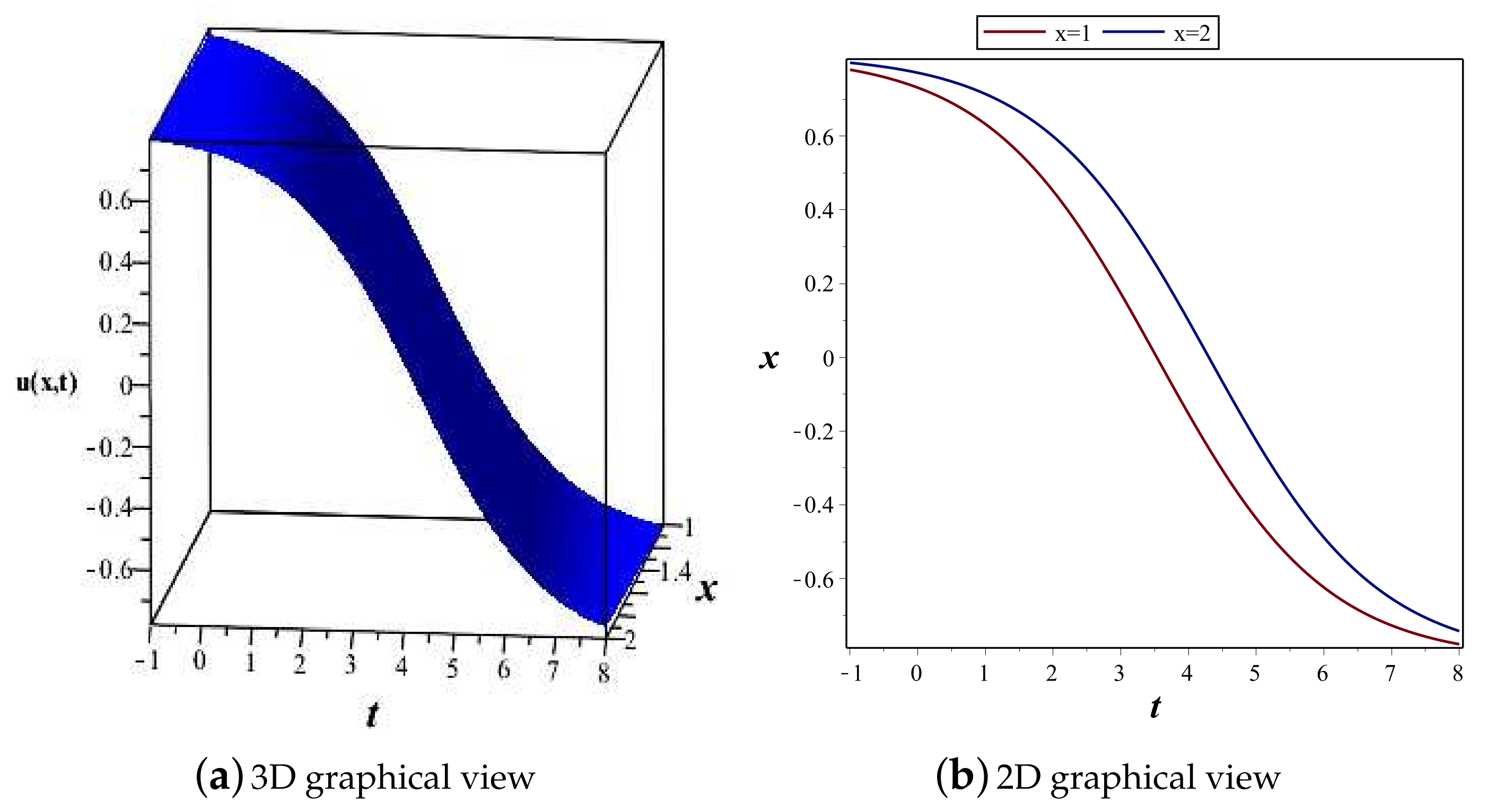
In this section, our focus is to define the physical behavior of traveling wave solutions which are obtained from governing equations. Figure 1, Figure 2 and Figure 3 illustrate the graphical behavior in 2D and 3D graphs of polynomial and rational function solutions of (RLW) Equation (8). Figure 4, Figure 5 and Figure 6 show the 2D and 3D graphs of polynomial and rational solution of (MRLW) Equation (27). Figure 7, Figure 8 and Figure 9 express the polynomial and rational solutions in 2D and 3D forms of (mZK) Equation (45). In the polynomial, Figure 1a,b and Figure 2a,b plot the graphs at different values of parameters, respectively ($a_2=4,$$b_2=1.4,v=2,\beta =1.2$), ($a_1=-0.3,a_2=2.4,v=3,\beta =2$). In the rational, Figure 3a,b plots a graph at constants ($c_0=1.3,c_1=2,c_2=3,a_2=1$, $v=-5$, $\beta =-1,$, $C=0$). For Equation (27), Figure 4a,b, Figure 5a,b and Figure 6a,b plot graphs at the given parameters ($a_0=-1.3,a_1=2.3,b_2=1.9,v=0.4,\beta =2$), ($a_0=-1,a_1=2.6,v=2,\beta =-2,C=1$) and ($a_0=1.9,a_1=2.3,c_0=2.8,c_1=2.8,v=1.3,\beta =-1.2,C=0$). Similarly, for (mZK) Equation (45), Figure 7a,b, Figure 8a,b and Figure 9a,b indicate the plot in 3D and 2D forms at the given parameters ($a_1=2.5,b_0=-0.2,b_1=1.4,b_2=1.8,v=1,y=2$), ($a_0=-2.3,a_1=2.4,y=2,v=1.4,\beta =-1.6,C=0$) and ($a_0=1,a_1=2.2,c_0=-2.4,c_1=1.3,c_2=2,v=-0.06,y=2,C=0$).

5. Advantages and Limitations

5.1. Advantages

• The unified method gives analytical solutions using traveling wave transformations.
• The proposed method provides us with multiple solutions of different types of governing equations with minimum effort.

5.2. Limitations

• The unified method is not applicable to linear PDEs due to the absence of a highest order nonlinear term.
• The proposed scheme is also not applicable to those equations which have a balancing number zero, such as the Zabolotskaya–Khokhlov (ZK) equation [38].

6. Conclusions

In this article, exact solutions of two nonlinear homogeneous partial differential equations, namely the generalized regularized long wave equation and modified Zakharov–Kuznetsov (mZK) equation, were investigated. For this purpose, we used different traveling wave transformations for finding the analytical solution in polynomial and rational forms. On the basis of traveling wave transformation, PDE was converted into ODE. The exact solution can be found by applying the unified method. Computer software, such as Maple and Mathematica, were used to solve the system of equations. This method provided us with an exact solution of the (GRLW) and (mZK) equations and also described their graphical representation in 2D and 3D forms using specific parameters. The unified method offers multiple solutions of different types with minimum effort.

References

- Osman, M.S. Multi-soliton rational solutions for quantum Zakharov-Kuznetsov equation in quantum magnetoplasmas. Waves Random Complex Media 2016, 26, 434–443. [Google Scholar] [CrossRef]
- Osman, M.S.; Baleanu, D.; Adem, A.R.; Hosseini, K.; Mirzazadeh, M.; Eslami, M. Double-wave solu-tions and Lie symmetry analysis to the (2 + 1)-dimensional coupled Burgers equations. Chin. J. Phys. 2020, 63, 122–129. [Google Scholar] [CrossRef]
- El-Sherif, A.A.; Shoukry, M.M. Equilibrium investigation of complex formation reactions involving copper (II), nitrilo-tris (methyl phosphonic acid) and amino acids, peptides or DNA constitutents. The kinetics, mechanism and correlation of rates with complex stability for metal ion promoted hydrolysis of glycine methyl ester. J. Coord. Chem. 2006, 59, 1541–1556. [Google Scholar]
- Soliman, A.A.; Amin, M.A.; El-Sherif, A.A.; Sahin, C.; Varlikli, C. Synthesis, characterization and molecular modeling of new ruthenium (II) complexes with nitrogen and nitrogen/oxygen donor ligands. Arab. J. Chem. 2017, 10, 389–397. [Google Scholar] [CrossRef]
- Ali, K.K.; Cattani, C.; Gómez-Aguilar, J.F.; Baleanu, D.; Osman, M.S. Analytical and numerical study of the DNA dynamics arising in oscillator-chain of Peyrard-Bishop model. Chaos Solitons Fractals 2020, 139, 110089. [Google Scholar] [CrossRef]
- Ding, Y.; Osman, M.S.; Wazwaz, A.M. Abundant complex wave solutions for the nonautonomous Fokas Lenells equation in presence of perturbation terms. Optik 2019, 181, 503–513. [Google Scholar] [CrossRef]
- Fan, E.; Hona, Y.C. Generalized tanh method extended to special types of nonlinear equations. Z. Naturforsch. A 2002, 57, 692–700. [Google Scholar] [CrossRef]
- He, J.H.; Wu, X.H. Exp-function method for nonlinear wave equations. Chaos Solitons Fractals 2006, 30, 700–708. [Google Scholar] [CrossRef]
- Zhang, S. Exp-function method exactly solving a KdV equation with forcing term. Appl. Math. Comput. 2008, 197, 128–134. [Google Scholar] [CrossRef]
- Akbar, M.A.; Ali, N.H.M.; Zayed, E.M.E. Abundant exact traveling wave solutions of generalized bretherton equation via improved (G’/G)-expansion method. Commun. Theor. Phys. 2012, 57, 173. [Google Scholar] [CrossRef]
- Alam, M.N.; Akbar, M.A.; Mohyud-Din, S.T. A novel (G’/G)-expansion method and its application to the Boussinesq equation. Chin. Phys. B 2013, 23, 020203. [Google Scholar] [CrossRef]
- Hasan, Q.M.U.; Naher, H.; Abdullah, F.; Mohyud-Din, S.T. Solutions of the nonlinear evolution equation via the generalized Riccati equation mapping together with the (G/G)-expansion method. J. Comput. Anal. Appl. 2016, 21, 62–82. [Google Scholar]
- Alam, M.N. Exact solutions to the foam drainage equation by using the new generalized G0/G-expansion method. Results Phys. 2015, 5, 168–177. [Google Scholar] [CrossRef]
- Wang, M.; Li, X.; Zhang, J. The (G’ G)-expansion method and travelling wave solutions of nonlinear evolution equations in mathematical physics. Phys. Lett. A 2008, 372, 417–423. [Google Scholar] [CrossRef]
- Conte, R.; Musette, M. Link between solitary waves and projective Riccati equations. J. Phys. A Math. Gen. 1992, 25, 5609. [Google Scholar] [CrossRef]
- Tanoglu, G. Solitary wave solution of nonlinear multi-dimensional wave equation by bilinear transformation method. Commun. Nonlinear Sci. Numer. Simul. 2007, 12, 1195–1201. [Google Scholar] [CrossRef]
- Hirota, R. Exact envelope-soliton solutions of a nonlinear wave equation. J. Math. Phys. 1973, 14, 805–809. [Google Scholar] [CrossRef]
- Hirota, R.; Satsuma, J. Soliton solutions of a coupled Korteweg-de Vries equation. Phys. Lett. A 1981, 85, 407–408. [Google Scholar] [CrossRef]
- Inc, M.; Kilic, B.; Karatas, E.; Akgul, A. Solitary wave solutions for the Sawada Kotera equation. J. Adv. Phys. 2017, 6, 288–293. [Google Scholar] [CrossRef]
- Inc, M.; Gencoglu, M.T.; Akgul, A. Application of extended Adomian decomposition method and ex-tended variational iteration method to Hirota Satsuma coupled kdv equation. J. Adv. Phys. 2017, 6, 216–222. [Google Scholar] [CrossRef]
- Mohammed, P.O.; Alqudah, M.A.; Hamed, Y.S.; Kashuri, A.; Abualnaja, K.M. Solving the modified regularized long wave equations via higher degree B–spline algorithm. J. Funct. Spaces 2021, 2021, 5580687. [Google Scholar] [CrossRef]
- Srivastava, H.M.; Gusu, D.M.; Mohammed, P.O.; Wedajo, G.; Nonlaopon, K.; Hamed, Y.S. Solutions of General Fractional–Order Differential Equations by Using the Spectral Tau Method. Fractal Fract. 2021, 6, 7. [Google Scholar] [CrossRef]
- Mohammed, P.O.; Machado, J.A.T.; Guirao, J.L.; Agarwal, R.P. Adomian decomposi-tion and fractional power series solution of a class of nonlinear fractional differential equations. Mathematics 2021, 9, 1070. [Google Scholar] [CrossRef]
- Srivastava, H.M.; Mohammed, P.O.; Guirao, J.L.; Hamed, Y.S. Some higher–degree Lacunary fractional splines in the approximation of fractional differential equations. Symmetry 2021, 13, 422. [Google Scholar] [CrossRef]
- Salas, A.H.; Gomez S, C.A. Application of the Cole Hopf transformation for finding exact so-lutions to several forms of the seventh-order KdV equation. Math. Probl. Eng. 2010, 2010, 194329. [Google Scholar] [CrossRef]
- Majeed, A.; Rafiq, M.N.; Kamran, M.; Abbas, M.; Inc, M. Analytical solutions of the fifth-order time fractional nonlinear evolution equations by the unified method. Mod. Phys. Lett. B 2022, 36, 2150546. [Google Scholar] [CrossRef]
- Raza, N.; Rafiq, M.H.; Kaplan, M.; Kumar, S.; Chu, Y.M. The unified method for abundant soliton solutions of local time fractional nonlinear evolution equations. Results Phys. 2021, 22, 103979. [Google Scholar] [CrossRef]
- Rafiq, M.N.; Majeed, A.; Yao, S.W.; Kamran, M.; Rafiq, M.H.; Inc, M. Analytical solutions of nonlinear time fractional evaluation equations via unified method with different derivatives and their comparison. Results Phys. 2021, 26, 104357. [Google Scholar] [CrossRef]
- Savovic, S.; Drljaca, B.; Djordjevich, A. A comparative study of two different finite difference methods for solving advection diffusion reaction equation for modeling exponential traveling wave in heat and mass transfer processes. Ric. Mat. 2021, 71, 245–252. [Google Scholar] [CrossRef]
- Pindza, E.; Mare, E. Solving the generalized regularized long wave equation using a distributed approximating functional method. Int. J. Comput. Math. 2014, 178024. [Google Scholar] [CrossRef]
- Ali, K.K.; Seadawy, A.R.; Yokus, A.; Yilmazer, R.; Bulut, H. Propagation of dispersive wave solu-tions for (3 + 1)-dimensional nonlinear modified Zakharov Kuznetsov equation in plasma physics. Int. J. Mod. Phys. B 2020, 34, 2050227. [Google Scholar] [CrossRef]
- Panahipour, H. Application of extended tanh method to generalized Burgers-type equations. Commun. Numer. Anal. 2012, 2012, 1–14. [Google Scholar] [CrossRef]
- Osman, M.S.; Korkmaz, A.; Rezazadeh, H.; Mirzazadeh, M.; Eslami, M.; Zhou, Q. The unified method for conformable time fractional Schro dinger equation with perturbation terms. Chin. J. Phys. 2018, 56, 2500–2506. [Google Scholar] [CrossRef]
- Seadawy, A.R. Three-dimensional nonlinear modified Zakharov Kuznetsov equation of ion-acoustic waves in a magnetized plasma. Comput. Math. Appl. 2016, 71, 201–212. [Google Scholar] [CrossRef]
- Khalfallah, M. New Exact Traveling Wave Solutions of the (2 + 1) dimensional Zakharov-Kuznetsov (ZK) Equation. Analele Stiint. Univ. Ovidius Constanta 2007, 15, 35–43. [Google Scholar]
- Bekir, A. Application of the (G’ G)-expansion method for nonlinear evolution equations. Phys. Lett. A 2008, 372, 3400–3406. [Google Scholar] [CrossRef]
- Islam, M.H.; Khan, K.; Akbar, M.A.; Salam, M.A. Exact traveling wave solutions of modified KdV Zakharov Kuznetsov equation and viscous Burgers equation. SpringerPlus 2014, 3, 105. [Google Scholar] [CrossRef]
- Bruzon, M.S.G.; Arias, M.L.; Torrisi, M.; Tracina, R. Some traveling wave solutions for the dissipative Zabolotskaya Khokhlov equation. J. Math. Phys. 2009, 50, 103504. [Google Scholar] [CrossRef]
Figure 1.
Graphical representation of Equation (17) within interval 5 ≤ x ≤ 7 and −2 ≤ t ≤ 9 (the (b) shows 2D plot for x = 5, 6).
Figure 2.
Graphical behavior of Equation (20) within interval 0.7 ≤ x ≤ 1.3 and −1 ≤ t ≤3 ((b) 2D plot for x = 0.7, 0.9).
Figure 3.
Graphical visualizations of Equation (26) within interval 0.7 ≤ x ≤ 2 and −2 ≤ t ≤ 1 ((a) 3D plot, (b) 2D plot for x = 1, 1.3).
Figure 4.
Graphical representation of Equation (36) within interval −1 ≤ x ≤ 5 and 4.5 ≤ t ≤ 5 ((a) 3D plot, (b) 2D plot for t = 4.5, 5).
Figure 5.
Graphical representation of Equation (39) within interval 2 ≤ x ≤ 5 and −3 ≤ t ≤ 7 ((a) 3D plot, (b) 2D plot for t = 4, 5).
Figure 6.
Graphical representation of Equation (44) within interval 1 ≤ x ≤ 2 and −1 ≤ t ≤ 8 ((a) 3D plot, (b) 2D plot for t = 1, 2).
Figure 7.
Graphical behavior of Equation (54) within interval −2 ≤ x ≤ 2.5 and 2 ≤ t ≤ 3 ((a) 3D plot, (b) 2D plot for t = 2.1, 2.7).
Figure 8.
Graphical representation of Equation (57) within interval 1 ≤ x ≤ 2.3 and 1 ≤ t ≤ 6 ((a) 3D plot, (b) 2D plot for x = 1.2, 1.6).
Figure 9.
Graphical representation of Equation (63) within interval −1 ≤ x ≤ 9 and 5.2 ≤ t ≤ 6.3 ((a) 3D plot, (b) 2D plot for t = 5.9).
Publisher’s Note: MDPI stays neutral with regard to jurisdictional claims in published maps and institutional affiliations. |
© 2022 by the authors. Licensee MDPI, Basel, Switzerland. This article is an open access article distributed under the terms and conditions of the Creative Commons Attribution (CC BY) license (https://creativecommons.org/licenses/by/4.0/).
Share and Cite
MDPI and ACS Style
Wang, X.; Javed, S.A.; Majeed, A.; Kamran, M.; Abbas, M. Investigation of Exact Solutions of Nonlinear Evolution Equations Using Unified Method. Mathematics 2022, 10, 2996. https://doi.org/10.3390/math10162996
AMA Style
Wang X, Javed SA, Majeed A, Kamran M, Abbas M. Investigation of Exact Solutions of Nonlinear Evolution Equations Using Unified Method. Mathematics. 2022; 10(16):2996. https://doi.org/10.3390/math10162996
Chicago/Turabian StyleWang, Xiaoming, Shehbaz Ahmad Javed, Abdul Majeed, Mohsin Kamran, and Muhammad Abbas. 2022. "Investigation of Exact Solutions of Nonlinear Evolution Equations Using Unified Method" Mathematics 10, no. 16: 2996. https://doi.org/10.3390/math10162996
Note that from the first issue of 2016, this journal uses article numbers instead of page numbers. See further details here.