Solution of the Thermoelastic Problem for a Two-Dimensional Curved Beam with Bimodular Effects

Abstract

In classical thermoelasticity, the bimodular effect of materials is rarely considered. However, all materials will present, in essence, different properties in tension and compression, more or less. The bimodular effect is generally ignored only for simple analysis. In this study, we theoretically analyze a two-dimensional curved beam with a bimodular effect and under mechanical and thermal loads. We first establish a simplified model on a subarea in tension and compression. On the basis of this model, we adopt the Duhamel similarity theorem to change the initial thermoelastic problem as an elasticity problem without the thermal effect. The superposition of the special solution and supplement solution of the Lamé displacement equation enables us to satisfy the boundary conditions and stress continuity conditions of the bimodular curved beam, thus obtaining a two-dimensional thermoelastic solution. The results indicate that the solution obtained can reduce to bimodular curved beam problems without thermal loads and to the classical Golovin solution. In addition, the bimodular effect on thermal stresses is discussed under linear and non-linear temperature rise modes. Specially, when the compressive modulus is far greater than the tensile modulus, a large compressive stress will occur at the inner edge of the curved beam, which should be paid with more attention in the design of the curved beams in a thermal environment.

1. Introduction

In the theory of thermoelasticity, it is generally assumed that materials that constitute the studied body are perfectly elastic, homogeneous and isotropic; thus, conventional analyses in classical elasticity [1] can also be used in the analysis of the theory of thermoelasticity. For example, in the theory of thermoelasticity, the establishment of the Lamé equation with displacement components as the fundamental variable and the obtainment of the corresponding solution can follow the routine mode from classical elasticity. However, if the bimodular effect of materials is newly added into the original thermoelasticity, existing analyses will encounter, more or less, differences and even difficulties. For a specific issue, our attention may focus on when the bimodular effect is newly introduced, where the impact on the existing results is, and how much it will be. In this study, we theoretically analyze a two-dimensional curved beam with bimodular effect under the combined action of thermal and mechanical loads. Thus, the review for the existing works will begin with the bimodular material model and the application of the proposed model in the analysis of structural elements, then the development of thermoelasticity, and lastly, several recent works concerning bimodular thermoelastic problems of structural elements.

Many investigations showed that the vast majority of materials [2,3], such as graphite, ceramics, rubber, concrete and certain biomedical materials, have tensile and compressive strains of different magnitudes when they are subjected to tensile and compressive stresses of the same magnitude. Jones [4] called these materials as bimodular materials or multimodulus materials. In the theoretical analysis of the engineering field, two material models are widely adopted. The first is the Bert model [5], which is established on the criterion of positive–negative signs in strains of the longitudinal fibers. Generally, this model is used in the analysis of orthotropic materials and laminated composites [6,7,8]. The second is the Ambartsumyan model [9], which is established on the criterion of principal stress’s positive–negative signs, and this model is mainly applicable to the analysis of isotropic materials. The existing studies showed that the application of the Ambartsumyan model in structural analysis is of particular significance, because it is the judgment on principal stress that determines whether a certain point in a structure is in tension or in compression. Our study is based on the latter model on principal stress.

For the purpose of representation of the stress–strain relation, Ambartsumyan [9] used two broken straight lines to linearize the bimodular model that is originally nonlinear, as shown in Figure 1, in which the principal stress is denoted by σ and the principal strain by ε. For this model, the basic assumptions are as follows: (1) The studied body is elastic, continuous, isotropic and homogeneous. (2) Small deformations are satisfied. (3) When the materials is tensile along a certain principal direction, Young’s modulus and Poisson’s ratio are taken as E⁺ and μ⁺, respectively; while the materials are compressive, Young’s modulus and Poisson’s ratio are taken as E⁻ and μ⁻, respectively. (4) For three-dimensional spatial problems, basic equations including the equilibrium equation, geometrical equation and physical equation are essentially the same as those of classical elasticity when three principal stresses are uniformly positive or uniformly negative, but when the signs of three principal stresses are different, except for the physical equation, the remaining two equations are the same as those of classical elasticity. (5) μ⁺/E⁺ = μ⁻/E⁻, which ensures symmetry of the flexibility matrix in the usage of the finite element method. Note that this is a restrictive assumption that loses sense when the absolute value of the Poisson’s ratio is zero or very small [9].

According to the bimodular material model described above, the constitutive relation of bimodular materials is established on the basis of the determined positive and negative signs of principal stresses, thus the principal stress must be known in advance. However, principal stresses are generally obtained as a final solving result, not as a known condition before solving. Thus, in most cases, it is difficult to know the stress state at a point and this is the motivation to analyze the bimodular mechanical behavior. Moreover, it is difficult to conduct experiments to describe the elastic coefficients in complex stress states during the construction of constitutive relations. Analytical solutions are available in some simple cases, although they only concern bending elements including beams and plates [10,11,12,13]. In complex problems, we have to resort to the finite element method on an iterative technique [14,15,16,17,18].

In the theory of thermoelasticity [19], the thermal effect on the governing equations is reflected in the constitutive relation, in which the modulus of elasticity and the Poisson’s ratio of materials are two important constants. The linear thermoelasticity is established on the linear supplement of thermal strains to the original mechanical strains. When arbitrary mass forces act on an object, we generally solve the thermoelastic problem by finding a solution to the Lamé equation. Therefore, many basic thermoelastic problems were solved within the scope of the theory of elasticity. This is the classical body force analogy that is referred to as the Duhamel similarity theorem, which may date back to Duhamel who made great contributions to this field in history.

With the development of the theory of thermoelasticity, some generalized thermoelastic models have been presented for transient responses in many applications (for example, low temperatures and ultra-fast lasers heating) where the classical theory of thermoelasticity fails. Some representative theories in this regard can be found in [20,21,22,23]. Green and Lindsay’s theory has been addressed for many types of media, in which Marin et al. [24] used this theory in dipolar thermoelastic bodies. However, besides the development of the theory itself, it is also important to apply the theory to the analysis of the engineering components, or more specifically, it is equally important to analyze the thermoelastic behavior of engineering structures, for example, the thermoelastic behavior of nanobeams [25], microbeams [26], composite beams [27] and laminated beams [28]. The bimodular material beams including straight beams and curved beams should also be incorporated into the thermoelastic analysis of structures.

Recently, Wen et al. [29] first obtained a two-dimensional thermoelastic solution of a bimodular beam under thermal and mechanical loads, in which the Duhamel similarity theorem was used to transform the thermoelastic problem into a pure elastic problem. For the thermal stress problems of bimodular functionally graded beams, the displacement method in the Duhamel similarity theorem is no longer usable; thus, Xue et al. [30] adopted the stress method to obtain one- and two-dimensional thermal stress solutions under different temperature rise patterns. For metal bars, Guo et al. [31] adopted the common strain suppression method to derive a one-dimensional thermal stress expression and used the Duhamel similarity theorem to derive a two-dimensional thermoelastic solution, in which the two important conditions, stress equilibrium conditions and strain compatibility conditions, were discussed.

In existing studies, the thermal stress problem of curved beams rarely involves a bimodular effect of materials, which seems insufficient. The originality of the presented work lies in the obtainment of a two-dimensional thermal stress solution of the bimodular curved beam, for the first time, based on the Duhamel similarity theorem. Although Wen et al. [29] adopted the same method, the studied objects in [29] are bimodular straight beams. Xue et al. [30] aimed at bimodular functionally graded straight beams, and the method used was the stress method, not the displacement method discussed here. At the same time, Guo et al. [31] dealt with a bimodular straight beam only under thermal load. None of the existing works involve the thermal stress of bimodular curved beams; this may be seen as a research motivation for this paper. However, the curved beam that is widely used in the engineering field is an important component of special form with an initial curvature. Compared with the analysis of a straight beam, the analysis of a curved beam is much more complicated due to the existence of the initial curvature, in addition to the introduction of a bimodular effect of the materials. In other words, the application of the Duhamel similarity theorem in bimodular curved beams is more complicated than that in bimodular straight beams, which may be easily seen from the next analysis.

In this study, we theoretically analyze a two-dimensional curved beam with bimodular effect and under the combined action of thermal and mechanical loads. To this end, this paper is organized as follows. First, the solving problem is described in Section 2. The mechanical model based on the subarea in tension and compression is established in Section 3. The analyses for the problem proposed, including the establishment of the Lamé displacement equation, the composition of the solution and the final solution in an axisymmetric case, are given in Section 4. The regression verification of the solution and comparison are presented in Section 5. In Section 6, some typical computational examples are given, in which the bimodular effect on the thermoelastic solution is discussed. The concluding remarks are presented in Section 7.

2. Problem Description

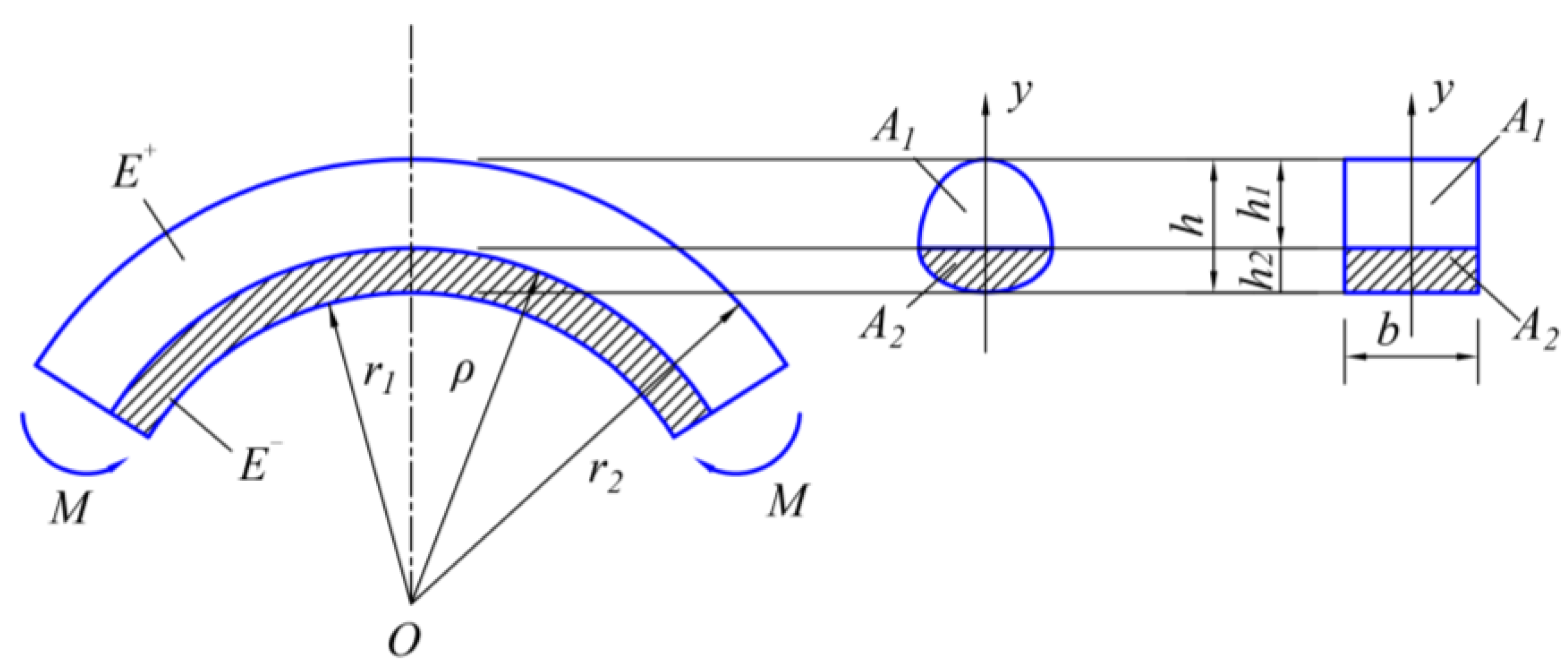
A bimodular curved beam with a certain section type and unit thickness is subjected to the bending moment, M, and the thermal load, T, and any segment in the beam is taken as a studied object, as shown in Figure 2, in which r₁ represents the inner radius of the curved beam, r₂ represents the outer radius, and ρ is the curvature radius of the neutral layer, which is unknown at present. For any point P of the beam, r represents its polar radius, and θ represents its polar angle, in which the positive rotation direction is specified as from the positive half x-axis to the positive half y-axis; that is, the positive rotation direction is clockwise, as shown in Figure 2. In this study, we adopt two-dimensional thermoelasticity to find thermal stresses of the bimodular curved beam under bending moment and thermal load. Under the action of external bending moment M, the curved beam further bends inward, generating an inner tensile area, as shown in the shading in Figure 2, and an outer compressive area. Our simplified mechanical model is established on the basis of a subarea in tension and compression.

3. Simplified Mechanical Model on Tension—Compression Subarea

The basic assumptions in the next analysis are as follows: (i) The initial neutral layer depends only on the bending moment, not on the thermal load, which is to say, the thermal load is applied after the action of the bending moment and the generation of the neutral layer. (ii) Similar to common shallow beams, the bending is limited in plane by a small-deflection bending without torsion. (iii) The material of the beam is considered to be perfectly elastic but with the bimodular effect. (iv) The temperature varies only with the radial direction of the curved beam, meaning T = T(r).

As indicated above, under the action of bending moment shown in Figure 2, the curved beam will further deflect inward to resist the external bending moment, thus resulting in compression for the inside part of the beam and in tension for the outside part. Correspondingly, the modulus of elasticity for the inside part is taken as E⁻ while the modulus for the outside part is taken as E⁺, while neglecting the tension–compression difference for the Poisson’s ratio μ and the line expansion coefficient α. Studies have shown that it is reasonable to ignore the tension–compression differences of the Poisson’s ratio, because it has less impact on the results, in addition to the beam problem in which the Poisson’s ratio is set as zero in the shallow beam case.

To realize the tension–compression subarea, we need to derive the formulas of the position of the unknown neutral layer of the bimodular curved beam under the bending moment alone, as shown in Figure 3. The section type of the curved beam may initially be arbitrary as long as the cross section is symmetrical to the y-axis, as shown in the middle of Figure 3, in which A₁ and A₂ are the tensile area and compressive area of the cross section, respectively. Especially, for the convenience of derivation, the section may be selected as rectangular, as shown in the right of Figure 3, in which h and b (=1) are the height and width of the section, respectively, and h₁ and h₂ are the tensile and compressive heights, respectively.

Following the above assumption, the external bending moment M is applied at the two ends of the beam, and at the same time, no external axial force N is applied here, as shown in Figure 3. The circumferential fiber in the outer part of the beam is tensile, while the circumferential fiber in the inner part of the beam is compressive; thus, the resultants of the circumferential stress σ_θ acting on the section are

$$N={\displaystyle {\int }_{A_1}^{}{\sigma }_{\theta }^{+}}dA+{\displaystyle {\int }_{A_2}^{}{\sigma }_{\theta }^{-}}dA=0$$

(1)

and

$$M={\displaystyle {\int }_{A_1}^{}y{\sigma }_{\theta }^{+}}dA+{\displaystyle {\int }_{A_2}^{}y{\sigma }_{\theta }^{-}}dA,$$

(2)

in which the symbol “+” denotes the tension while the symbol ”−” denotes the compression.

Figure 4 shows the geometrical relation of a segment taken from the curved beam, in which dθ denotes the central angle of this segment, and δdθ denotes the change of central angle after deformation. Thus, the arc length of the circumferential fiber with a distance y from the neutral layer is (y + ρ) dθ. After deformation, this arc length elongates by yδdθ along the circumferential direction. Under the assumption of plane section, the relative elongation of the circumferential fiber is

$${\epsilon }_{\theta }=\frac{y}{y+\rho }\frac{\delta d\theta }{d\theta }.$$

(3)

Thus, according to Hooke’s law, in the tensile part, 0 ≤ y ≤ r₂ − ρ, we have

$${\sigma }_{\theta }^{+}=E^{+}\frac{y}{y+\rho }\frac{\delta d\theta }{d\theta },$$

(4)

while in the compressive part, r₁ − ρ ≤ y ≤ 0, we have

$${\sigma }_{\theta }^{-}=E^{-}\frac{y}{y+\rho }\frac{\delta d\theta }{d\theta }.$$

(5)

Substituting Equations (4) and (5) into Equations (1) and (2), we have

$$E^{+}{\displaystyle {\int }_{A_1}^{}\frac{y}{y+\rho }}dA+E^{-}{\displaystyle {\int }_{A_2}^{}\frac{y}{y+\rho }}dA=0,$$

(6)

which is used for determining the neutral layer and

$$\frac{\delta d\theta }{d\theta }\left[E^{+}{\displaystyle {\int }_{A_1}^{}\frac{y^2}{y+\rho }}dA+E^{-}{\displaystyle {\int }_{A_2}^{}\frac{y^2}{y+\rho }}dA\right]=M$$

(7)

or alternatively,

$$\frac{\delta d\theta }{d\theta }\left[E^{+}\left({\displaystyle {\int }_{A_1}^{}ydA}-{\displaystyle {\int }_{A_1}^{}\frac{y\rho }{y+\rho }}dA\right)+E^{-}\left({\displaystyle {\int }_{A_2}^{}ydA}-{\displaystyle {\int }_{A_2}^{}\frac{y\rho }{y+\rho }}dA\right)\right]=M.$$

(8)

If we note the relation from Equation (6), Equation (8) may be simplified as

$$\frac{\delta d\theta }{d\theta }=\frac{M}{E^{+}{\displaystyle {\int }_{A_1}^{}ydA}+E^{-}{\displaystyle {\int }_{A_2}^{}ydA}}.$$

(9)

Substituting Equation (9) into Equations (4) and (5) yields, for 0 ≤ y ≤ r₂ − ρ,

$${\sigma }_{\theta }^{+}=\frac{y}{y+\rho }\frac{M}{{\displaystyle {\int }_{A_1}^{}ydA}+\frac{E^{-}}{E^{+}}{\displaystyle {\int }_{A_2}^{}ydA}},$$

(10)

and for r₁ − ρ ≤ y ≤ 0,

$${\sigma }_{\theta }^{-}=\frac{y}{y+\rho }\frac{M}{\frac{E^{+}}{E^{-}}{\displaystyle {\int }_{A_1}^{}ydA}+{\displaystyle {\int }_{A_2}^{}ydA}}.$$

(11)

Thus, we obtain the tensile and compressive circumferential stresses.

Furthermore, Equation (6) may be changed as

$$E^{+}{\displaystyle {\int }_{A_1}^{}\left(1-\frac{\rho }{y+\rho }\right)}dA+E^{-}{\displaystyle {\int }_{A_2}^{}\left(1-\frac{\rho }{y+\rho }\right)}dA=0;$$

(12)

this gives

$$E^{+}{A}_1+E^{-}{A}_2=\rho E^{+}{\displaystyle {\int }_{A_1}^{}\frac{1}{y+\rho }}dA+\rho E^{-}{\displaystyle {\int }_{A_2}^{}\frac{1}{y+\rho }}dA.$$

(13)

If the section type of the cross section of the curved beam is rectangular, as shown in Figure 3, then the area of A₁ and A₂ may be computed as A₁ = r₂ − ρ and A₂ = ρ − r₁ (note that b = 1). The integral containing the variable y in Equation (13) may be transformed into the integral containing the polar radius r (see Figure 3), and thus Equation (13) may be written as

$$E^{+}(r_2-\rho )+E^{-}(\rho -r_1)=\rho E^{+}{\displaystyle {\int }_{\rho }^{r_2}\frac{1}{r}}dr+\rho E^{-}{\displaystyle {\int }_{r_1}^{\rho }\frac{1}{r}}dr.$$

(14)

After a simple computation, we obtain

$$\frac{E^{+}}{E^{-}}(r_2-\rho )+\rho -r_1-\frac{E^{+}}{E^{-}}\rho \ln \frac{r_2}{\rho }-\rho \ln \frac{\rho }{r_1}=0.$$

(15)

If we specify the ratio of E⁺ to E⁻ and the ratio of r₁ to r₂, Equation (15) may be used for the determination of ρ. The unknown neutral layer is found; thus, the simplified mechanical model based on a subarea in tension and compression is finally established.

4. Problem Solution

4.1. Displacement Governing Equation

In this section, we adopt the displacement method to solve the thermoelastic problem. As indicated above, the problem we consider here is a typical plane stress problem concerning thermal effect. In the polar coordinate system, if we let ε_r, ε_θ and γ_rθ be the strains of plane stress problems and σ_r, σ_θ and τ_rθ be the corresponding stresses, α represents the linear thermal expansion coefficient, and T represents the temperature variation. The physical equation of two-dimensional thermoelectricity will give [1]

$$\{\begin{array}{l}{\epsilon }_r=\frac{1}{E^{+/-}}\left({\sigma }_r-\mu {\sigma }_{\theta }\right)+\alpha T\\ {\epsilon }_{\theta }=\frac{1}{E^{+/-}}\left({\sigma }_{\theta }-\mu {\sigma }_r\right)+\alpha T\\ {\gamma }_{r\theta }=\frac{2(1+\mu )}{E^{+/-}}{\tau }_{r\theta }\end{array},$$

(16)

in which the tensile and compressive Young’s moduli are denoted by E^+/− for the time being, since in this case, there is no method to determine in advance whether the stress state of any point is tensile or compressive. For the physical equation, we may have another form as follows:

$$\{\begin{array}{l}{\sigma }_r=\frac{E^{+/-}}{1-{\mu }^2}({\epsilon }_r+\mu {\epsilon }_{\theta })-\frac{\alpha T{E}^{+/-}}{1-\mu }\\ {\sigma }_{\theta }=\frac{E^{+/-}}{1-{\mu }^2}({\epsilon }_{\theta }+\mu {\epsilon }_r)-\frac{\alpha T{E}^{+/-}}{1-\mu }\\ {\tau }_{r\theta }=\frac{E^{+/-}}{2(1+\mu )}{\gamma }_{r\theta }\end{array}.$$

(17)

If we let u_r and u_θ be the displacement along r and θ direction, respectively, the geometrical equation of the plane problem gives [1]

$$\{\begin{array}{l}{\epsilon }_r=\frac{\partial u_r}{\partial r}\\ {\epsilon }_{\theta }=\frac{u_r}{r}+\frac{1}{r}\frac{\partial u_{\theta }}{\partial \theta }\\ {\gamma }_{r\theta }=\frac{1}{r}\frac{\partial u_r}{\partial \theta }+\frac{\partial u_{\theta }}{\partial r}-\frac{u_{\theta }}{r}\end{array}.$$

(18)

Substituting Equation (18) into Equation (17), the stress components expressed in terms of the u_r, u_θ and T may be obtained as

$$\{\begin{array}{l}{\sigma }_r=\frac{E^{+/-}}{1-{\mu }^2}\left[\frac{\partial u_r}{\partial r}+\mu \left(\frac{u_r}{r}+\frac{1}{r}\frac{\partial u_{\theta }}{\partial \theta }\right)\right]-\frac{E^{+/-}\alpha T}{1-\mu }\\ {\sigma }_{\theta }=\frac{E^{+/-}}{1-{\mu }^2}\left(\frac{u_r}{r}+\frac{1}{r}\frac{\partial u_{\theta }}{\partial \theta }+\mu \frac{\partial u_r}{\partial r}\right)-\frac{E^{+/-}\alpha T}{1-\mu }\\ {\tau }_{r\theta }=\frac{E^{+/-}}{2\left(1+\mu \right)}\left(\frac{1}{r}\frac{\partial u_r}{\partial \theta }+\frac{\partial u_{\theta }}{\partial r}-\frac{u_{\theta }}{r}\right)\end{array}.$$

(19)

If we let K_r and K_θ be the body forces along the radial and circumferential direction, respectively, the equation of equilibrium of the plane problem gives [1]

$$\{\begin{array}{l}\frac{\partial {\sigma }_r}{\partial r}+\frac{1}{r}\frac{\partial {\tau }_{r\theta }}{\partial \theta }+\frac{{\sigma }_r-{\sigma }_{\theta }}{r}+K_r=0\\ \frac{1}{r}\frac{\partial {\sigma }_{\theta }}{\partial \theta }+\frac{\partial {\tau }_{r\theta }}{\partial r}+\frac{2{\tau }_{r\theta }}{r}+K_{\theta }=0\end{array}.$$

(20)

Substituting Equation (19) into Equation (20), the Lamé equation used for the displacement method may be obtained as follows

$$\{\begin{array}{l}\frac{E^{+/-}}{1-{\mu }^2}\left[\frac{{\partial }^2{u}_r}{\partial r^2}+\frac{1-\mu }{2r^2}\frac{{\partial }^2{u}_r}{\partial {\theta }^2}+\frac{1+\mu }{2r}\frac{{\partial }^2{u}_{\theta }}{\partial r\partial \theta }+\frac{1}{r}\frac{\partial u_r}{\partial r}+\frac{\mu -3}{2r^2}\frac{\partial u_{\theta }}{\partial \theta }-\frac{u_r}{r^2}\right]\\ -\frac{E\alpha }{1-\mu }\frac{\partial T}{\partial r}=0\\ \frac{E^{+/-}}{1-{\mu }^2}\left[\frac{1}{r^2}\frac{{\partial }^2{u}_{\theta }}{\partial {\theta }^2}+\frac{1-\mu }{2}\frac{{\partial }^2{u}_{\theta }}{\partial r^2}+\frac{1+\mu }{2r}\frac{{\partial }^2{u}_r}{\partial r\partial \theta }+\frac{3-\mu }{2r^2}\frac{\partial u_r}{\partial \theta }+\frac{1-\mu }{2r}\frac{\partial u_{\theta }}{\partial r}+\frac{\mu -1}{2}\frac{u_{\theta }}{r^2}\right]\\ -\frac{E\alpha }{1-\mu }\frac{1}{r}\frac{\partial T}{\partial \theta }=0\end{array},$$

(21)

in which K_r and K_θ are prescribed as zero.

In addition, the stress boundary conditions of the plane problem are [1]

$$\{\begin{array}{l}l{({\sigma }_r)}_s+m{({\tau }_{r\theta })}_s={\overline{f}}_r\\ m{({\sigma }_{\theta })}_s+l{({\tau }_{r\theta })}_s={\overline{f}}_{\theta }\end{array},$$

(22)

in which l and m are the direction cosines, and ${\overline{f}}_r$ and ${\overline{f}}_{\theta }$ are the surfaces forces. Substituting Equation (19) into the above equation, we will have the stress boundary conditions used for the displacement method (noting ${\overline{f}}_r={\overline{f}}_{\theta }=0$)

$$\{\begin{array}{l}l{\left[\frac{\partial u_r}{\partial r}+\mu \left(\frac{u_r}{r}+\frac{1}{r}\frac{\partial u_{\theta }}{\partial \theta }\right)\right]}_s+m\frac{1-\mu }{2}{\left(\frac{1}{r}\frac{\partial u_r}{\partial \theta }+\frac{\partial u_{\theta }}{\partial r}-\frac{u_{\theta }}{r}\right)}_s=l\left(1+\mu \right)\alpha T\\ m{\left(\frac{u_r}{r}+\frac{1}{r}\frac{\partial u_{\theta }}{\partial \theta }+\mu \frac{\partial u_r}{\partial r}\right)}_s+l\frac{1-\mu }{2}{\left(\frac{1}{r}\frac{\partial u_r}{\partial \theta }+\frac{\partial u_{\theta }}{\partial r}-\frac{u_{\theta }}{r}\right)}_s=m\left(1+\mu \right)\alpha T\end{array}.$$

(23)

Therefore, we derive the Lamé equation and corresponding boundary conditions in the polar coordinate system, that is, Equations (21) and (23), which are used for the displacement method of the two-dimensional thermoelastic problem.

Comparing Equations (21) and (23) with the counterparts in the plane stress problem without thermal effect, we may find such a fact that the original body forces, K_r and K_θ, are now replaced by the following formulas

$$\{\begin{array}{l}{K}_r\to -\frac{E^{+/-}\alpha }{1-\mu }\frac{\partial T}{\partial r}\\ K_{\theta }\to -\frac{E^{+/-}\alpha }{1-\mu }\frac{1}{r}\frac{\partial T}{\partial \theta }\end{array},$$

(24)

while at the same time, the original surface forces, ${\overline{f}}_r$ and ${\overline{f}}_{\theta }$ are now replaced by

$$\{\begin{array}{l}{\overline{f}}_r\to l\frac{E^{+/-}\alpha T}{1-\mu }\\ {\overline{f}}_{\theta }\to m\frac{E^{+/-}\alpha T}{1-\mu }\end{array}.$$

(25)

This fact suggests that although the bimodular effect is introduced in this study, under certain displacement boundary conditions, the displacement due to temperature variation T is equal to the displacement of the elastic body without temperature variation, which is subjected to the imaginary body forces shown in Equation (24) and the imaginary surface forces shown in Equation (25). Therefore, the thermoelastic plane stress problem with the bimodular effect may also be transformed into a pure elasticity problem under the known body forces and known surface forces; this is the Duhamel similarity theorem we are familiar with.

4.2. Composition of Solution

Generally, under the stress boundary condition (23) and displacement boundary condition, it is difficult for us to obtain the analytical solution of the displacement governing Equation (21). Therefore, in an actual solving process, it is a common practice to follow the next two steps. First, we need to find any special solution of Equation (21) that may not satisfy the boundary conditions. Second, not considering temperature changes, another supplement solution is found. By superposing the supplement solution on the previous special solution, the total stress is finally obtained to satisfy the boundary conditions.

To find the special solution of Equation (21), a potential function of displacement, $\psi (r,\theta )$, is introduced here, and the special solution of displacement may be adopted as

$$u_r\prime =\frac{\partial \psi }{\partial r}, u_{\theta }\prime =\frac{1}{r}\frac{\partial \psi }{\partial \theta }.$$

(26)

Regarding $u_r\prime$ and $u_{\theta }\prime$ as u_r and u_θ, substituting them into Equation (21) yields

$$\{\begin{array}{l}\frac{\partial }{\partial r}{\nabla }^2\psi =\left(1+\mu \right)\alpha \frac{\partial T}{\partial r}\\ \frac{1}{r}\frac{\partial }{\partial \theta }{\nabla }^2\psi =\left(1+\mu \right)\alpha \frac{1}{r}\frac{\partial T}{\partial \theta }\end{array}.$$

(27)

Note that μ and α are both constants in this problem, which shows if the function $\psi (r,\theta )$ can satisfy the following differential equation

$${\nabla }^2\psi =(1+\mu )\alpha T,$$

(28)

in which

$${\nabla }^2=\frac{{\partial }^2}{\partial r^2}+\frac{1}{r}\frac{\partial }{\partial r}+\frac{1}{r^2}\frac{{\partial }^2}{\partial {\theta }^2},$$

(29)

then $\psi (r,\theta )$ can satisfy Equation (27), thus also satisfying Equation (21). Eventually, $u_r\prime$ and $u_{\theta }\prime$ may be regarded as a special solution of displacement. By substituting Equations (26) and (28) into Equation (19), we may have the stress component corresponding to the special solution

$$\{\begin{array}{l}{\sigma }_r\prime =-\frac{E^{+/-}}{1+\mu }\left(\frac{1}{r}\frac{\partial \psi }{\partial r}+\frac{1}{r^2}\frac{{\partial }^2\psi }{\partial {\theta }^2}\right)\\ {\sigma }_{\theta }\prime =-\frac{E^{+/-}}{1+\mu }\frac{{\partial }^2\psi }{\partial r^2}\\ {\tau }_{r\theta }\prime =\frac{E^{+/-}}{1+\mu }\frac{\partial }{\partial r}\left(\frac{1}{r}\frac{\partial \psi }{\partial \theta }\right)\end{array}.$$

(30)

Meanwhile, the supplement solution of displacement $u_r″$ and $u_{\theta }″$ need to satisfy the homogeneous form of Equation (21), such that

$$\{\begin{array}{l}\frac{{\partial }^2{u}_r}{\partial r^2}+\frac{1-\mu }{2r^2}\frac{{\partial }^2{u}_r}{\partial {\theta }^2}+\frac{1+\mu }{2r}\frac{{\partial }^2{u}_{\theta }}{\partial r\partial \theta }+\frac{1}{r}\frac{\partial u_r}{\partial r}+\frac{\mu -3}{2r^2}\frac{\partial u_{\theta }}{\partial \theta }-\frac{u_r}{r^2}=0\\ \frac{1}{r^2}\frac{{\partial }^2{u}_{\theta }}{\partial {\theta }^2}+\frac{1-\mu }{2}\frac{{\partial }^2{u}_{\theta }}{\partial r^2}+\frac{1+\mu }{2r}\frac{{\partial }^2{u}_r}{\partial r\partial \theta }+\frac{3-\mu }{2r^2}\frac{\partial u_r}{\partial \theta }+\frac{1-\mu }{2r}\frac{\partial u_{\theta }}{\partial r}+\frac{\mu -1}{2}\frac{u_{\theta }}{r^2}=0\end{array}.$$

(31)

By using Equation (19) and also letting T = 0, we have the stress components corresponding to the supplement solution of displacement,

$$\{\begin{array}{l}{\sigma }_r″=\frac{E^{+/-}}{1-{\mu }^2}\left[\frac{\partial u_r″}{\partial r}+\mu \left(\frac{u_r″}{r}+\frac{1}{r}\frac{\partial u_{\theta }″}{\partial \theta }\right)\right]\\ {\sigma }_{\theta }″=\frac{E^{+/-}}{1-{\mu }^2}\left(\frac{u_r″}{r}+\frac{1}{r}\frac{\partial u_{\theta }″}{\partial \theta }+\mu \frac{\partial u_r″}{\partial r}\right)\\ {\tau }_{r\theta }″=\frac{E^{+/-}}{2\left(1+\mu \right)}\left(\frac{1}{r}\frac{\partial u_r″}{\partial \theta }+\frac{\partial u_{\theta }″}{\partial r}-\frac{u_{\theta }″}{r}\right)\end{array}.$$

(32)

Lastly, the total displacements are

$$u_r=u_r\prime +u_r″,u_{\theta }=u_{\theta }\prime +u_{\theta }″,$$

(33)

which need to satisfy displacement boundary conditions. In addition, the total stress are

$$\{\begin{array}{l}{\sigma }_r={\sigma }_r\prime +{\sigma }_r″\\ {\sigma }_{\theta }={\sigma }_{\theta }\prime +{\sigma }_{\theta }″\\ {\tau }_{r\theta }={\tau }_{r\theta }\prime +{\tau }_{r\theta }″ \end{array},$$

(34)

which need to satisfy stress boundary conditions.

4.3. Solution in Axisymmetric Case

4.3.1. Special Solution

In an axisymmetric problem, if the temperature variation is also axisymmetric, that is, T = T(r), it is easy for us to obtain the special solution according to the description above. In this case, the displacement potential function may be simplified as $\psi =\psi (r)$; thus, the differential Equation (28), of which the $\psi (r)$ should satisfy now, becomes

$$\left(\frac{d^2}{d{r}^2}+\frac{1}{r}\frac{d}{dr}\right)\psi =\left(1+\mu \right)\alpha T$$

(35)

or alternatively,

$$\frac{1}{r}\frac{d}{dr}\left(r\frac{d\psi }{dr}\right)=\left(1+\mu \right)\alpha T.$$

(36)

Integrating the above formula with respect to r twice, we have

$$\psi (r)=\left(1+\mu \right)\alpha {\displaystyle \int \frac{1}{r}}{\displaystyle \int Trdr}dr+\left(1+\mu \right)\alpha D_1\ln r+D_2$$

(37)

in which D₁ and D₂ are two integral constants, and for the convenience of the next computation, the factor (1 + μ) α is multiplied before the constant D₁. Substituting Equation (37) into Equation (30), we have the stress components corresponding to displacement special solution as follows

$$\{\begin{array}{l}{\sigma }_r\prime =-\frac{E^{+/-}}{1+\mu }\frac{1}{r}\frac{d\psi }{dr}=-\frac{E^{+/-}\alpha }{r^2}\left({\displaystyle \int Trdr}+D\right)\\ {\sigma }_{\theta }\prime =-\frac{E^{+/-}}{1+\mu }\frac{d^2\psi }{d{r}^2}=\frac{E^{+/-}\alpha }{r^2}\left({\displaystyle \int Trdr}+D-T{r}^2\right)\\ {\tau }_{r\theta }\prime =0\end{array}.$$

(38)

in which D₂ disappear, and for simplicity, D₁ has been changed to D. Note that in the above equation, the upper limit of the integral should be the variable r, while the lower limit of the integral may be arbitrarily selected, according to the real problem. In this study, r₁ and r₂ are the inner radius and outer radius of the curved beam, respectively (see Figure 2); thus, the lower limit of the integral is r₁. In addition, according to our previous study [29], the stress in the special solution always corresponds to the compressive stress; thus, the E^+/− in Equation (38) should be modified as E⁻, according to the bimodular characteristics described above. Finally, the stress components corresponding to the displacement special solution becomes

$$\{\begin{array}{l}{\sigma }_r\prime =-\frac{E^{-}\alpha }{r^2}\left({\displaystyle {\int }_{r_1}^{r}T}rdr+D\right)\\ {\sigma }_{\theta }\prime =\frac{E^{-}\alpha }{r^2}\left({\displaystyle {\int }_{r_1}^{r}T}rdr+D-T{r}^2\right)\\ {\tau }_{r\theta }\prime =0\end{array}.$$

(39)

It is easy to see that this special solution cannot satisfy the boundary conditions shown in Figure 2, that is, σ_r is zero not only at r₁ but also at r₂. By observing the ${\sigma }_r\prime$ in Equation (39), it was found that there is no way to find such a constant D that satisfies the two conditions simultaneously. Therefore, seeking the supplement solution of displacement is necessary.

4.3.2. Supplement Solution

To obtain the supplement solution, we need to adopt the stress function method, that is, to introduce a stress function, ϕ(r,θ), which should satisfy the following consistency equation

$${\left(\frac{{\partial }^2}{\partial r^2}+\frac{1}{r}\frac{\partial }{\partial r}+\frac{1}{r^2}\frac{{\partial }^2}{\partial {\theta }^2}\right)}^2\phi =0.$$

(40)

The corresponding stress components, that is, the supplement solution, will become [1]

$$\{\begin{array}{l}{\sigma }_r″=\frac{1}{r}\frac{\partial \phi }{\partial r}+\frac{1}{r^2}\frac{{\partial }^2\phi }{\partial {\theta }^2}\\ {\sigma }_{\theta }″=\frac{{\partial }^2\phi }{\partial r^2}\\ {\tau }_{r\theta }″=-\frac{\partial }{\partial r}\left(\frac{1}{r}\frac{\partial \phi }{\partial \theta }\right)\end{array}.$$

(41)

However, it is still hard to determine the specific form of the ϕ(r,θ). Due to the axisymmetric stress problem of the present study, we now have ϕ = ϕ(r); thus, Equation (40) may be simplified as

$${\left(\frac{d^2}{d{r}^2}+\frac{1}{r}\frac{d}{dr}\right)}^2\phi =0,$$

(42)

or alternatively,

$$\frac{1}{r}\frac{d}{dr}\left\{r\frac{d}{dr}\left[\frac{1}{r}\frac{d}{dr}\left(r\frac{d\phi }{dr}\right)\right]\right\}=0.$$

(43)

Integrating with respect to r four times, we may obtain [1]

$$\phi =A\ln r+B{r}^2\ln r+C{r}^2+G,$$

(44)

in which A, B, C and G are four integral constants. Here, we adopt the mechanical model on the subarea in tension and compression; thus, the stress components should be given in the form of tensile and compressive parts. Substituting Equation (44) into Equation (41), we have the stress components expressed in terms of the unknown constants that distinguish between tension and compression. Specifically, for the tensile part, ρ ≤ r ≤ r₂,

$$\{\begin{array}{l}{\sigma }_r^{+}″=\frac{1}{r}\frac{d{\phi }^{+}}{dr}=\frac{A^{+}}{r^2}+B^{+}\left(1+2\ln r\right)+2C^{+}\\ {\sigma }_{\theta }^{+}″=\frac{d^2{\phi }^{+}}{d{r}^2}=-\frac{A^{+}}{r^2}+B^{+}\left(3+2\ln r\right)+2C^{+}\\ {\tau }_{r\theta }^{+}″=0\end{array},$$

(45)

and for the compressive part, r₁ ≤ r ≤ ρ,

$$\{\begin{array}{l}{\sigma }_r^{-}″=\frac{1}{r}\frac{d{\phi }^{-}}{dr}=\frac{A^{-}}{r^2}+B^{-}\left(1+2\ln r\right)+2C^{-}\\ {\sigma }_{\theta }^{-}″=\frac{d^2{\phi }^{-}}{d{r}^2}=-\frac{A^{-}}{r^2}+B^{-}\left(3+2\ln r\right)+2C^{-}\\ {\tau }_{r\theta }^{-}″=0\end{array}.$$

(46)

in which the quantities with superscript ‘+’ denote the tension, and the quantities with superscript ‘−’ denote the compression.

4.3.3. Superposition of Two Solutions

Now, superposing the special solution on the supplement solution, that is, by adding Equations (39) and (45)–(46), we have, for ρ ≤ r ≤ r₂,

$$\{\begin{array}{l}{\sigma }_r^{+}=-\frac{E^{-}\alpha }{r^2}\left[{\displaystyle {\int }_{r_1}^{r}T}rdr+D\right]+\frac{A^{+}}{r^2}+B^{+}\left(1+2\ln r\right)+2C^{+}\\ {\sigma }_{\theta }^{+}=\frac{E^{-}\alpha }{r^2}\left[{\displaystyle {\int }_{r_1}^{r}T}rdr+D-T{r}^2\right]-\frac{A^{+}}{r^2}+B^{+}\left(3+2\ln r\right)+2C^{+}\\ {\tau }_{r\theta }^{+}={\tau }_{\theta r}^{+}=0\end{array},$$

(47)

and for r₁ ≤ r ≤ ρ,

$$\{\begin{array}{l}{\sigma }_r^{-}=-\frac{E^{-}\alpha }{r^2}\left[{\displaystyle {\int }_{r_1}^{r}T}rdr+D\right]+\frac{A^{-}}{r^2}+B^{-}\left(1+2\ln r\right)+2C^{-}\\ {\sigma }_{\theta }^{-}=\frac{E^{-}\alpha }{r^2}\left[{\displaystyle {\int }_{r_1}^{r}T}rdr+D-T{r}^2\right]-\frac{A^{-}}{r^2}+B^{-}\left(3+2\ln r\right)+2C^{-}\\ {\tau }_{r\theta }^{-}={\tau }_{\theta r}^{-}=0\end{array},$$

(48)

Note that after the subarea is in tension and compression, the number of undetermined constants is basically redoubled, from the original three to six, except for the constant D. Not only the stress boundary conditions but also the stress continuity conditions need to be combined to determine the seven unknown constants, A^+/−, B^+/−, C^+/− and D.

The total stresses should satisfy the following boundary conditions: at the inner edge of the curved beam, first, we have

$${\sigma }_r^{-}=0, {\tau }_{r\theta }^{-}=0 \mathrm{at} r=r_1.$$

(49)

Substituting the first one of Equation (48) into the above condition will give

$$-\frac{E^{-}\alpha }{r_1^2}\left[{\displaystyle {\int }_{r_1}^{r_1}T}rdr+D\right]+\frac{A^{-}}{r_1^2}+B^{-}\left(1+2\ln r_1\right)+2C^{-}=0,$$

(50)

which is simplified as, noting that the integral in Equation (50) is zero,

$$\frac{A^{-}}{r_1^2}+B^{-}\left(1+2\ln r_1\right)+2C^{-}=\frac{E^{-}\alpha }{r_1^2}D.$$

(51)

At the outer edge of the curved beam, we have

$${\sigma }_r^{+}=0, {\tau }_{r\theta }^{+}=0 \mathrm{at} r=r_2.$$

(52)

Substituting the first one of Equation (47) into the above condition will give

$$-\frac{E^{-}\alpha }{r_2^2}\left[{\displaystyle {\int }_{r_1}^{r_2}T}rdr+D\right]+\frac{A^{+}}{r_2^2}+B^{+}\left(1+2\ln r_2\right)+2C^{+}=0.$$

(53)

If we let

$$J_1={\displaystyle {\int }_{r_1}^{r_2}T}rdr$$

(54)

Equation (53) may be written as

$$\frac{A^{+}}{r_2^2}+B^{+}\left(1+2\ln r_2\right)+2C^{+}=\frac{E^{-}\alpha }{r_2^2}\left(J_1+D\right).$$

(55)

Due to the fact that r₁ or r₂ is far greater than the section height h of the curved beam, the de Saint-Venant Principle may be used to formulate the boundary conditions at any end of the curved beam, this gives

$$\{\begin{array}{l}{\displaystyle {\int }_{\rho }^{r_2}{\sigma }_{\theta }^{+}dr}+{\displaystyle {\int }_{r_1}^{\rho }{\sigma }_{\theta }^{-}dr}=0\\ {\displaystyle {\int }_{\rho }^{r_2}{\sigma }_{\theta }^{+}rdr}+{\displaystyle {\int }_{r_1}^{\rho }{\sigma }_{\theta }^{-}rdr}=0\\ {\displaystyle {\int }_{\rho }^{r_2}{\tau }_{r\theta }^{+}dr}+{\displaystyle {\int }_{r_1}^{\rho }{\tau }_{r\theta }^{-}dr}=0\end{array}.$$

(56)

In addition, the stress continuity conditions on the neutral layer should be

$${\sigma }_r^{+}={\sigma }_r^{-} \mathrm{at} r=\rho ,$$

(57)

and

$${\sigma }_{\theta }^{+}={\sigma }_{\theta }^{-}=0,{ }_{}^{}\mathrm{at} r=\rho .$$

(58)

First, the third integral of Equation (56) is naturally satisfied. Substituting the second one of Equations (47) and (48) into the first integral of Equation (56) will give

$$\begin{array}{l}{\displaystyle {\int }_{\rho }^{r_2}\left[\frac{E^{-}\alpha }{r^2}\left({\displaystyle {\int }_{r_1}^{r}T}rdr+D-T{r}^2\right)-\frac{A^{+}}{r^2}+B^{+}\left(3+2\ln r\right)+2C^{+}\right]dr}\\ +{\displaystyle {\int }_{r_1}^{\rho }\left[\frac{E^{-}\alpha }{r^2}\left({\displaystyle {\int }_{r_1}^{r}T}rdr+D-T{r}^2\right)-\frac{A^{-}}{r^2}+B^{-}\left(3+2\ln r\right)+2C^{-}\right]dr}=0\end{array}$$

(59)

Noting that the terms containing A^+/−, B^+/− and C^+/− in the above integral may be written as [32], according to Equations (45) and (46),

$$\begin{array}{l}{\displaystyle {\int }_{\rho }^{r_2}\frac{d^2{\phi }^{+}}{d{r}^2}}dr+{\displaystyle {\int }_{r_1}^{\rho }\frac{d^2{\phi }^{-}}{d{r}^2}}dr={\left[\frac{d{\phi }^{+}}{dr}\right]}_{\rho }^{r_2}+{\left[\frac{d{\phi }^{-}}{dr}\right]}_{r_1}^{\rho }={\left[r{\sigma }_r^{+}\right]}_{\rho }^{r_2}+{\left[r{\sigma }_r^{-}\right]}_{r_1}^{\rho }\\ =r_2{\left[{\sigma }_r^{+}\right]}_{r=r_2}-\rho {\left[{\sigma }_r^{+}\right]}_{r=\rho }+\rho {\left[{\sigma }_r^{-}\right]}_{r=\rho }-r_1{\left[{\sigma }_r^{-}\right]}_{r=r_1}\end{array}$$

(60)

If we note Equations (49), (52) and (57), it is easy to see that the above integral is zero, and the two integrals in Equation (59) may be combined due to the same integrands; thus, Equation (59) may be further simplified as

$$E^{-}\alpha {\displaystyle {\int }_{r_1}^{r_2}\left(\frac{1}{r^2}{\displaystyle {\int }_{r_1}^{r}T}rdr+\frac{1}{r^2}D-T\right)dr}=0.$$

(61)

If we let

$$J_2={\displaystyle {\int }_{r_1}^{r_2}T}dr$$

(62)

and

$$J_3={\displaystyle {\int }_{r_1}^{r_2}\frac{1}{r^2}{\displaystyle {\int }_{r_1}^{r}T}}rdrdr,$$

(63)

Equation (61) becomes

$$J_3-D\left(\frac{1}{r_2}-\frac{1}{r_1}\right)-J_2=0.$$

(64)

Substituting the second one of Equations (47) and (48) into the second integral of Equation (56) will give

$$\begin{array}{l}{\displaystyle {\int }_{\rho }^{r_2}\left[\frac{E^{-}\alpha }{r^2}\left({\displaystyle {\int }_{r_1}^{r}T}rdr+D-T{r}^2\right)-\frac{A^{+}}{r^2}+B^{+}\left(3+2\ln r\right)+2C^{+}\right]rdr}\\ +{\displaystyle {\int }_{r_1}^{\rho }\left[\frac{E^{-}\alpha }{r^2}\left({\displaystyle {\int }_{r_1}^{r}T}rdr+D-T{r}^2\right)-\frac{A^{-}}{r^2}+B^{-}\left(3+2\ln r\right)+2C^{-}\right]rdr}=M\end{array}$$

(65)

Similarly, noting that the terms containing A^+/−, B^+/− and C^+/− in the above integral may be written as [32], according to Equations (45) and (46),

$$\begin{array}{l}{\displaystyle {\int }_{\rho }^{r_2}\frac{d^2{\phi }^{+}}{d{r}^2}}rdr+{\displaystyle {\int }_{r_1}^{\rho }\frac{d^2{\phi }^{-}}{d{r}^2}}rdr={\displaystyle {\int }_{\rho }^{r_2}rd\left(\frac{d{\phi }^{+}}{dr}\right)}+{\displaystyle {\int }_{r_1}^{\rho }rd\left(\frac{d{\phi }^{-}}{dr}\right)}\\ ={\left[r^2{\sigma }_r^{+}\right]}_{\rho }^{r_2}-{\left[{\phi }^{+}\right]}_{\rho }^{r_2}+{\left[r^2{\sigma }_r^{-}\right]}_{r_1}^{\rho }-{\left[{\phi }^{-}\right]}_{r_1}^{\rho }\\ =r_2^2{\left[{\sigma }_r^{+}\right]}_{r=r_2}-{\rho }^2{\left[{\sigma }_r^{+}\right]}_{r=\rho }-{\left[{\phi }^{+}\right]}_{\rho }^{r_2}+{\rho }^2{\left[{\sigma }_r^{-}\right]}_{r=\rho }-r_1^2{\left[{\sigma }_r^{-}\right]}_{r=r_1}-{\left[{\phi }^{-}\right]}_{r_1}^{\rho }\end{array}$$

(66)

If we note Equations (49), (52) and (57), it is easy to see that in the above integral, only $-{[{\phi }^{+}]}_{\rho }^{r_2}-{[{\phi }^{-}]}_{r_1}^{\rho }$ remain, and the two integrals in Equation (65) may be combined due to the same integrands; thus, Equation (65) becomes

$${\displaystyle {\int }_{r_1}^{r_2}\left[\frac{E^{-}\alpha }{r^2}\left({\displaystyle {\int }_{r_1}^{r}T}rdr+D-T{r}^2\right)\right]rdr}-{[{\phi }^{+}]}_{\rho }^{r_2}-{[{\phi }^{-}]}_{r_1}^{\rho }=M.$$

(67)

If we let

$$J_4={\displaystyle {\int }_{r_1}^{r_2}\frac{1}{r}{\displaystyle {\int }_{r_1}^{r}T}}rdrdr,$$

(68)

and also noting Equations (44) and (54), Equation (67) becomes

$$\begin{array}{l}{A}^{+}\ln \frac{r_2}{\rho }+B^{+}\left(r_2{}^2\ln r_2-{\rho }^2\ln \rho \right)+C^{+}\left(r_2{}^2-{\rho }^2\right)\\ +A^{-}\ln \frac{\rho }{r_1}+B^{-}\left({\rho }^2\ln \rho -r_1{}^2\ln r_1\right)+C^{-}\left({\rho }^2-r_1{}^2\right)=E^{-}\alpha \left(J_4+D\ln \frac{r_2}{r_1}+J_1\right)-M\end{array}$$

(69)

For the stress continuity conditions, substituting the first one of Equations (47) and (48) into Equation (57) will give

$$\frac{A^{+}}{{\rho }^2}+B^{+}\left(1+2\ln \rho \right)+2C^{+}=\frac{A^{-}}{{\rho }^2}+B^{-}\left(1+2\ln \rho \right)+2C^{-}.$$

(70)

In addition, substituting the second one of Equations (47) and (48) into Equation (58) will give

$$-\frac{A^{+}}{{\rho }^2}+B^{+}\left(3+2\ln \rho \right)+2C^{+}=0,$$

(71)

and

$$-\frac{A^{-}}{{\rho }^2}+B^{-}\left(3+2\ln \rho \right)+2C^{-}=0,$$

(72)

in which the stress terms concerning thermal load are not considered since the neutral layer of the beam is determined only under the action of external bending moment M, as indicated in our previous assumption in Section 3.

Finally, Equations (51), (55), (64) and (69)–(72), in total, seven in number, are used for the solution of the seven undetermined constants, A^+/−, B^+/−, C^+/− and D. For the solving process in detail, refer to Appendix A.

5. Regression Verification and Comparison

5.1. Reduction to Bimodular Problem

In this section, let us verify if the solution obtained may reduce to the existing bimodular problem. Supposing that there is no temperature variation, that is, T(r) = 0, we may have the following simple relations, by referring to Appendix A,

$$\{\begin{array}{l}{J}_1=J_2=J_3=J_4=0,D=(J_3-J_2)\frac{r_1{r}_2}{r_1-r_2}=0\\ F_1=\frac{E^{-}\alpha }{r^2}\left(J_1+D\right)=0,F_2=\frac{E^{-}\alpha }{r_1{}^2}D=0\\ F_3=E^{-}\alpha (J_4+D\ln \frac{r_2}{r_1}+J_1)=0\end{array},$$

(73)

thus

$$K_1=K_2=K_3=K_4=K_5=K_6=0.$$

(74)

A^+/−, B^+/− and C^+/− now become

$$\{\begin{array}{l}{A}^{+}=\frac{4M{P}_1}{R}{\rho }^2{r}_2{}^2(\ln \frac{r_2}{\rho }-1)\hspace{1em}{A}^{-}=\frac{4M{P}_2}{R}{\rho }^2{r}_1{}^2(\ln \frac{r_1}{\rho }-1)\\ B^{+}=-\frac{2M{P}_1}{R}({\rho }^2+r_2{}^2)\hspace{1em}{B}^{-}=-\frac{2M{P}_2}{R}({\rho }^2+r_1{}^2)\\ C^{+}=\frac{M{P}_1}{R}[{\rho }^2(3+2\ln \rho )+r_2{}^2(1+2\ln r_2)]\\ C^{-}=\frac{M{P}_2}{R}[{\rho }^2(3+2\ln \rho )+r_1{}^2(1+2\ln r_1)]\end{array}.$$

(75)

which is exactly the solution from He et al. [32], in which P₁, P₂ and R are the same as those in [32], according to Equation (A4). This agreement verifies the correctness of the solution obtained in this study from the side.

5.2. Reduction to Classical Golovin Solution

The above reduction seems insufficient to verify the correctness of the solution; we may further derive the solution without the bimodular effect, to demonstrate the rationality of the solving process presented in this study. For this purpose, we first give the stress formulas as, corresponding to Equations (47) and (48),

$$\{\begin{array}{l}{\sigma }_r=-\frac{E\alpha }{r^2}\left({\displaystyle {\int }_{r_1}^{r}T}rdr+D\right)+\frac{A}{r^2}+B\left(1+2\ln r\right)+2C\\ {\sigma }_{\theta }=\frac{E\alpha }{r^2}\left({\displaystyle {\int }_{r_1}^{r}T}rdr+D-T{r}^2\right)-\frac{A}{r^2}+B\left(3+2\ln r\right)+2C\\ {\tau }_{r\theta }={\tau }_{r\theta }=0\end{array},$$

(76)

in which only four constants, A, B, C and D, need to be determined. The boundary conditions are listed as follows

$$\{\begin{array}{l}{\sigma }_r=0, r=r_1, r_2\\ {\displaystyle {\int }_{r_1}^{r_2}{\sigma }_{\theta }dr}=0\\ {\displaystyle {\int }_{r_1}^{r_2}{\sigma }_{\theta }rdr}=M\end{array}.$$

(77)

The above four boundary conditions are sufficient to determine A, B, C and D. Substituting Equation (76) into Equation (77), we may obtain the following four equations used for the determination of A, B, C and D,

$$\{\begin{array}{l}\frac{A}{r_1{}^2}+B\left(1+2\ln r_1\right)+2C=\frac{E\alpha }{r_1{}^2}D\\ \frac{A}{r_2{}^2}+B\left(1+2\ln r_2\right)+2C=\frac{E\alpha }{r_2{}^2}\left(J_1+D\right)\\ J_3-D\left(\frac{1}{r_2}-\frac{1}{r_1}\right)-J_2=0\\ A\ln \frac{r_2}{r_1}+B\left(r_2{}^2\ln r_2-r_1{}^2\ln r_1\right)+C\left(r_2{}^2-r_1{}^2\right)=E\alpha \left(J_4+D\ln \frac{r_2}{r_1}+J_1\right)-M\end{array},$$

(78)

which gives

$$\{\begin{array}{l}A=\frac{4\left(F_3-M\right)r_1^2{r}_2^2\ln \left(r_1/r_2\right)}{N{r}_1^4}+\frac{\left(F_1-F_2\right)r_1^2{r}_2^2\left(r_1{}^2-r_2{}^2\right)+2F_2{r}_1^2{r}_2^4\ln \left(r_2/r_1\right)-2F_1{r}_1^4{r}_2^2\ln \left(r_2/r_1\right)}{N{r}_1^4}\\ B=\frac{2\left(F_3-M\right)\left(r_1{}^2-r_2{}^2\right)}{N{r}_1^4}+\frac{\left(F_1{r}_1{}^2-F_2{r}_2{}^2\right)\left(r_1{}^2-r_2{}^2\right)+2\left(F_1-F_2\right)r_1{}^2{r}_2{}^2\ln \left(r_2/r_1\right)}{N{r}_1^4}\\ C=\frac{\left(F_3-M\right)\left[2\left(r_2{}^2\ln r_2-r_1{}^2\ln r_1\right)-\left(r_1{}^2-r_2{}^2\right)\right]}{N{r}_1^4}\\ -\frac{\left(F_1{r}_1{}^2-F_2{r}_2{}^2\right)\left(r_1{}^2\ln r_1-r_2{}^2\ln r_2\right)+r_1{}^2{r}_2{}^2\ln \left(r_2/r_1\right)\left[F_1-F_2+2\left(F_1\ln r_2-F_2\ln r_1\right)\right]}{N{r}_1^4}\\ D=\left(J_3-J_2\right)\frac{r_2{r}_1}{r_1-r_2}\end{array},$$

(79)

in which

$$\{\begin{array}{l}{F}_1=\frac{E\alpha }{r^2}(J_1+D)\\ F_2=\frac{E\alpha }{r_1{}^2}D\\ F_3=E\alpha (J_4+D\ln \frac{r_2}{r_1}+J_1)\\ N=\frac{{\left(r_1{}^2-r_2{}^2\right)}^2-4r_1{}^2{r}_2{}^2{\ln }^2\left(r_2/r_1\right)}{r_1^4}\end{array}.$$

(80)

When T(r) = 0, we still have

$$\{\begin{array}{l}{J}_1=J_2=J_3=J_4=0\\ D=0\\ F_1=F_2=F_3=0\end{array}.$$

(81)

Substituting them into Equations (79) and (76), we obtain the classical Golovin solution [1] as follows

$$\{\begin{array}{l}{\sigma }_r=-\frac{4M}{N{r}_1^2}\left(\frac{r_2{}^2}{r_1{}^2}\ln \frac{r_2}{r}+\ln \frac{r}{r_1}-\frac{r_2{}^2}{r^2}\ln \frac{r_2}{r_1}\right)\\ {\sigma }_{\theta }=\frac{4M}{N{r}_1^2}\left(\frac{r_2{}^2}{r_1{}^2}-1-\frac{r_2{}^2}{r_1{}^2}\ln \frac{r_2}{r}-\ln \frac{r}{r_1}-\frac{r_2{}^2}{r^2}\ln \frac{r_2}{r_1}\right)\\ {\tau }_{r\theta }={\tau }_{\theta r}=0\end{array}.$$

(82)

which verifies again, from the aspect of the solving method, the correctness of the solution obtained.

Due to the lack of the other solution to the same problem in the existing work, whether an analytical solution or numerical one, the verification of the solution is only conducted on the basis of the satisfaction of regression. The satisfaction at least guarantees the necessity condition of the correct solution, but it is not a condition of sufficiency. Follow-up work will focus on the verification to the condition of sufficiency, and from this point of view, the numerical simulation of practical problems may be a solution.

6. Bimodular Effect on Thermal Stress

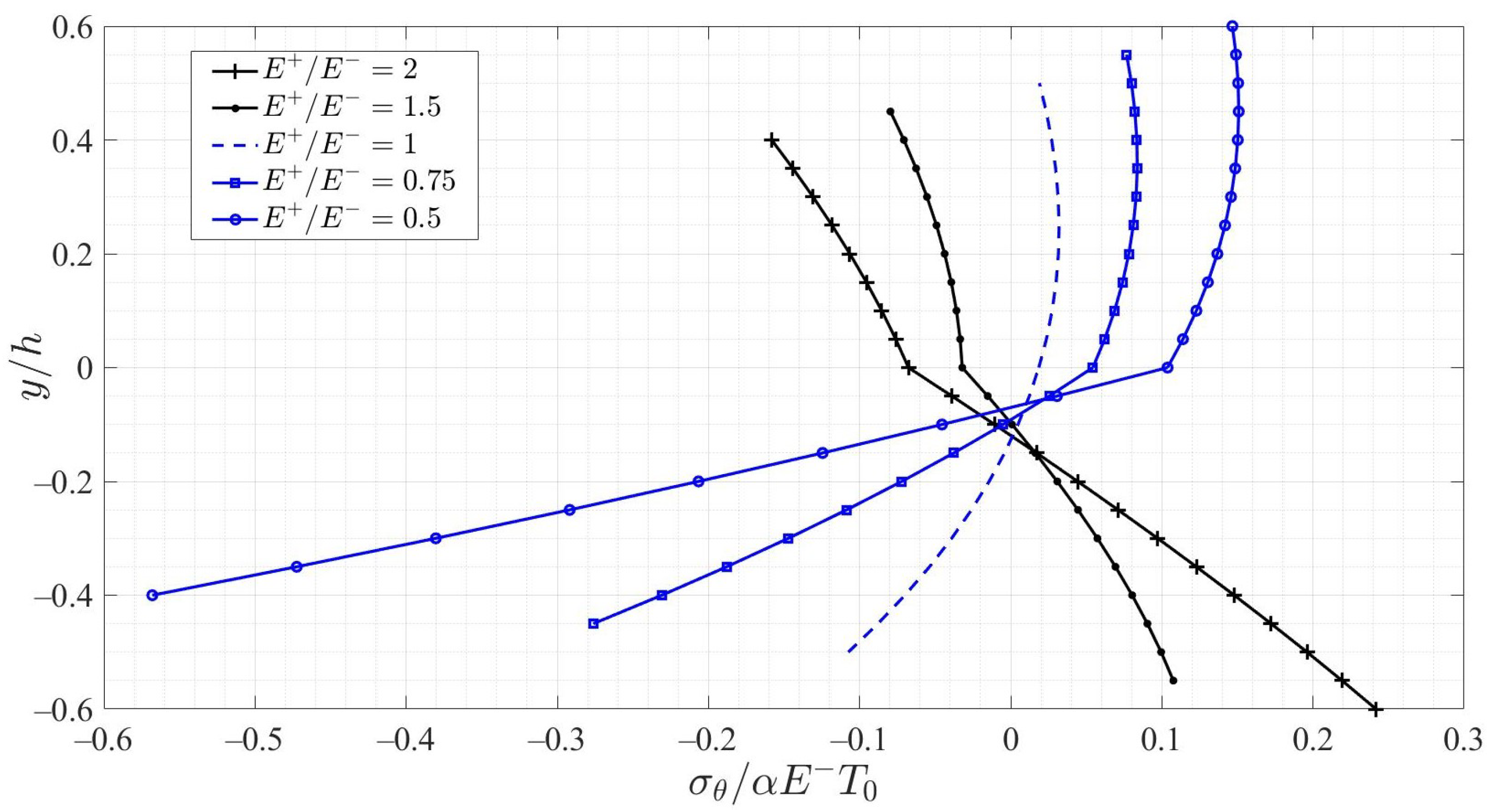
In order to study the bimodular effect on the thermal stress σ_θ, the five bimodular cases are considered: (1) E⁺ = 2E⁻, (2) E⁺ = 1.5E⁻, (3) E⁺ = E⁻, (4) E⁺ = 0.75E⁻ and (5) E⁺ = 0.5E⁻, in which the first two cases belong to E⁺ > E⁻, while the latter two cases belong to E⁺ < E⁻. Considering that the curved beam is relatively shallow, the values of r₁/r₂ are taken as 0.80. Thus, according to Equation (15), the positions for the unknown neutral layers, which is given in the form of dimensionless quantities, ρ/r₂, are computed and listed in

Table 1. Neutral layer positions for five bimodular cases when r₁/r₂ = 0.8.

Bimodular Cases	Tensile Modulus	Compressive Modulus	ρ/r2
E+ = 2E−	2E−	E−	0.913539
E+ = 1.5E	1.5E−	E−	0.906417
E+ = E−	E−	E−	0.896284
E+ = 0.75E−	0.75E−	E−	0.889128
E+ = 0.5E−	0.5E−	E−	0.879248

.

According to our previous studies on thermal stresses of bimodular beams [30,31,32], one-dimensional solutions on the strain suppression method are basically consistent with two-dimensional thermoelastic solutions. Given that the thermoelastic solution obtained in this study is too complex to be conveniently used for numerical analysis, we have to resort to the one-dimensional solution to discuss the bimodular effect on the thermal stress, in which the mechanical load, that is, the bending moment M, is set to zero to focus our attention on the thermal stress introduced only by the temperature load.

According to the strain suppression method [1] and Equations (10) and (11) derived in this work, the thermal stress σ_θ in the tensile and compression areas may be easily determined as (please refer to Figure 3), for the tensile area, 0 ≤ y ≤ h₁ (in which h₁ = r₂ − ρ)

$${\sigma }_{\theta }^{+}=-\alpha E^{-}T(y)+\frac{1}{A}{\displaystyle {\int }_{-h_2}^{h_1}\alpha E^{-}T(y)bdy}+\frac{y}{y+\rho }\frac{{\displaystyle {\int }_{-h_2}^{h_1}\alpha E^{-}T(y)bydy}}{{\displaystyle {\int }_{A_1}^{}ydA}+\frac{E^{-}}{E^{+}}{\displaystyle {\int }_{A_2}^{}ydA}},$$

(83)

and for the compressive area, −h₂ ≤ y ≤ 0 (in which h₂ = ρ − r₁)

$${\sigma }_{\theta }^{-}=-\alpha E^{-}T(y)+\frac{1}{A}{\displaystyle {\int }_{-h_2}^{h_1}\alpha E^{-}T(y)bdy}+\frac{y}{y+\rho }\frac{{\displaystyle {\int }_{-h_2}^{h_1}\alpha E^{-}T(y)bydy}}{\frac{E^{+}}{E^{-}}{\displaystyle {\int }_{A_1}^{}ydA}+{\displaystyle {\int }_{A_2}^{}ydA}}.$$

(84)

From Equations (83) and (84), in the one-dimensional solutions on the strain suppression method, there are basically three terms that give clear physical meanings, and they are the compressive stress due to initial strain suppression, the axial tensile stress that counteracts the compression applied before, and the bending stress that also counteracts the compression applied in the first step. Note that in the above equations, the basic variable is y but not r, and if the rectangular section type is considered here, we may have the area A = bh, the tensile height h₁ = r₂ − ρ and the compressive height h₂ = ρ − r₁. Thus, we may further compute the integral on the denominator in Equations (83) and (84), and obtain, for 0 ≤ y ≤ h₁,

$${\sigma }_{\theta }^{+}=-\alpha E^{-}T(y)+\frac{1}{h}{\displaystyle {\int }_{-h_2}^{h_1}\alpha E^{-}T(y)dy}+\frac{y}{y+\rho }\frac{2E^{+}{\displaystyle {\int }_{-h_2}^{h_1}\alpha E^{-}T(y)ydy}}{E^{+}{(r_2-\rho )}^2-E^{-}{(r_1-\rho )}^2},$$

(85)

and for −h₂ ≤ y ≤ 0,

$${\sigma }_{\theta }^{-}=-\alpha E^{-}T(y)+\frac{1}{h}{\displaystyle {\int }_{-h_2}^{h_1}\alpha E^{-}T(y)dy}+\frac{y}{y+\rho }\frac{2E^{-}{\displaystyle {\int }_{-h_2}^{h_1}\alpha E^{-}T(y)ydy}}{E^{+}{(r_2-\rho )}^2-E^{-}{(r_1-\rho )}^2}.$$

(86)

If we further give the function form of T(y), for example, T(y) = T₀f(y/h), Equations (85) and (86) may be changed as the dimensionless form, for 0 ≤ y/h ≤ h₁/h,

$$\frac{{\sigma }_{\theta }^{+}}{\alpha E^{-}{T}_0}=-f(y/h)+\frac{1}{h}{\displaystyle {\int }_{-h_2}^{h_1}f(y/h)dy}+\frac{y}{y+\rho }\frac{2E^{+}{\displaystyle {\int }_{-h_2}^{h_1}f(y/h)ydy}}{E^{+}{(r_2-\rho )}^2-E^{-}{(r_1-\rho )}^2},$$

(87)

and for h₂/h ≤ y/h ≤ 0,

$$\frac{{\sigma }_{\theta }^{-}}{\alpha E^{-}{T}_0}=-f(y/h)+\frac{1}{h}{\displaystyle {\int }_{-h_2}^{h_1}f(y/h)dy}+\frac{y}{y+\rho }\frac{2E^{-}{\displaystyle {\int }_{-h_2}^{h_1}f(y/h)ydy}}{E^{+}{(r_2-\rho )}^2-E^{-}{(r_1-\rho )}^2}.$$

(88)

Now, we prescribe two different temperature rise modes, the linear and the non-linear, to plot the variation curves of the dimensionless thermal stress σ_θ/αE⁻T₀ with y/h, under different bimodular cases, as shown in Figure 5 and Figure 6, in which the x-axis stands for the dimensionless stress σ_θ/αE⁻T₀ and the y-axis for the dimensionless section height y/h. The linear and non-linear temperature rise modes are defined as, respectively,

$$T(y)=T_{0}f(y)=T_0\frac{y+h_2}{h}$$

(89)

and

$$T(y)=T_{0}f(y)=T_0\frac{e^{(y+h_2)/h}-1}{e-1}$$

(90)

which both satisfy the outer edge of the curved beam, that is, y = h₁, T(y) = T₀, and at the inner edge of the curved beam, that is, y = −h₂, T(y) = 0.

From Figure 5 and Figure 6:

(i)

Except for the case E⁺ = E⁻ whose curves are continuous and smooth, other curves from all bimodular cases will lose their smoothness on the neutral layer; this phenomenon is consistent with the bimodular material model shown in Figure 1.

(ii)

Regardless of the temperature change modes, the distribution of thermal stress is essentially nonlinear, which may be easily observed from Equations (87) and (88). However, if the temperature rise mode is non-linear, the curves from Figure 6 present relatively obvious nonlinear characteristics. Compared to the curves from Figure 5 under the linear temperature rise mode, the curvature of the curves becomes somewhat larger.

(iii)

Under the given temperature change modes, that is, from the inner edge of the curved beam to the outer edge, the temperature variation is from 0 to T₀; the tensile and compressive stresses occurring in different zones are also different for the bimodular cases. Especially, if E⁺ > E⁻, from the inner edge to the outer edge, the change of thermal stress status is basically from compression to tension; if E⁺ < E⁻, also from the inner edge to the outer edge, the situation is the opposite; the change in thermal stress status is basically from tension to compression. If E⁺ = E⁻, the stress transformation in tension and compression is slightly complicated. For the linear temperature rise mode, from the inner edge to the outer edge, the stress change is from compression to tension, while for the non-linear mode, the stress first experiences a compressive status, then changes to a tensile status, and finally returns to the compressive status.

(iv)

For the case E⁺ > E⁻, the change of stress status from tension to compression is moderate, but for the case E⁺ < E⁻, the change of stress status is quite drastic; this phenomenon may be easily observed from Figure 5 and Figure 6. Especially for the case of E⁺/E⁻ = 0.5, the maximum compressive stress approaches −0.58, indicating that when the compressive modulus is far greater than the tensile modulus, a large unexpected compressive stress will occur on the inner edge of the curved beam, which must be given sufficient attention to in the design of the curved beam with a bimodular effect in a thermal environment.

7. Concluding Remarks

In this paper, based on the simplified model on the subarea in tension and compression, we theoretically analyzed a two-dimensional curved beam with bimodular effect and under the combined action of thermal and mechanical loads. The following conclusions can be drawn.

(i)

Similar to the bimodular straight beam case, the Duhamel similarity theorem based on the body force and surface force analogy is still applicable to the bimodular curved beam, which enables us to transform the thermoelastic problem to a classical elastic problem.

(ii)

The obtainment of the solution was still established on the superposition of a special solution and supplement solution of the Lamé equation; however, due to the introduction of the bimodular effect, the superposed solution needs to satisfy the boundary conditions on the inner and outer edges as well as the stress continuity conditions on the neutral layer, simultaneously.

(iii)

The thermoelastic solution obtained may reduce not only to the bimodular curved beam but also to the classical Golovin solution, which verifies, from the side, the correctness of the solving.

(iv)

The introduction of the bimodular effect will bring great change to the thermal stress. If E⁺ > E⁻, from the inner edge to the outer edge of the curved beam, the change of thermal stress status is basically from compression to tension; if E⁺ < E⁻, the situation is the opposite. Specially, when the compressive modulus is far greater than the tensile modulus, a large unexpected compressive stress will occur on the inner edge of the curved beam, which should be given sufficient attention to in the design of a bimodular curved beam in a thermal environment.

In addition, due to the fact that the verification of the presented method of the solution is based on the regression of the solution by neglecting the temperature variation, the verification is somewhat insufficient. In subsequent work, the precise numerical simulation based on the finite element method may be adopted to realize the verification. The related work is being planned.

References

- Timoshenko, S.P.; Goodier, J.N. Theory of Elasticity, 3rd ed.; McGraw Hill: New York, NY, USA, 1970. [Google Scholar]
- Barak, M.M.; Currey, J.D.; Weiner, S.; Shahar, R. Are tensile and compressive Young’s moduli of compact bone different. J. Mech. Behav. Biomed. Mater. 2009, 2, 51–60. [Google Scholar] [CrossRef] [PubMed]
- Destrade, M.; Gilchrist, M.D.; Motherway, J.A.; Murphy, J.G. Bimodular rubber buckles early in bending. Mech. Mater. 2010, 42, 469–476. [Google Scholar] [CrossRef]
- Jones, R.M. Apparent flexural modulus and strength of multimodulus materials. J. Compos. Mater. 1976, 10, 342–354. [Google Scholar] [CrossRef]
- Bert, C.W. Models for fibrous composites with different properties in tension and compression. ASME J. Eng. Mater. Technol. 1977, 99, 344–349. [Google Scholar] [CrossRef]
- Reddy, J.N.; Chao, W.C. Nonlinear bending of bimodular material plates. Int. J. Solids Struct. 1983, 19, 229–237. [Google Scholar] [CrossRef]
- Zinno, R.; Greco, F. Damage evolution in bimodular laminated composite under cyclic loading. Compos. Struct. 2001, 53, 381–402. [Google Scholar] [CrossRef]
- Khan, A.H.; Patel, B.P. Nonlinear periodic response of bimodular laminated composite annular sector plates. Compos. Part B-Eng. 2019, 169, 96–108. [Google Scholar] [CrossRef]
- Ambartsumyan, S.A. Elasticity Theory of Different Moduli; Wu, R.F.; Zhang, Y.Z., Translators; China Railway Publishing House: Beijing, China, 1986. [Google Scholar]
- Yao, W.J.; Ye, Z.M. Analytical solution for bending beam subject to lateral force with different modulus. Appl. Math. Mech. 2004, 25, 1107–1117. [Google Scholar]
- Zhao, H.L.; Ye, Z.M. Analytic elasticity solution of bi-modulus beams under combined loads. Appl. Math. Mech. 2015, 36, 427–438. [Google Scholar] [CrossRef]
- He, X.T.; Sun, J.Y.; Wang, Z.X.; Chen, Q.; Zheng, Z.L. General perturbation solution of large-deflection circular plate with different moduli in tension and compression under various edge conditions. Int. J. Non-Linear Mech. 2013, 55, 110–119. [Google Scholar] [CrossRef]
- He, X.T.; Cao, L.; Wang, Y.Z.; Sun, J.Y.; Zheng, Z.L. A biparametric perturbation method for the Föppl-von Kármán equations of bimodular thin plates. J. Math. Anal. Appl. 2017, 455, 1688–1705. [Google Scholar] [CrossRef]
- Ye, Z.M.; Chen, T.; Yao, W.J. Progresses in elasticity theory with different moduli in tension and compression and related FEM. Mech. Eng. 2004, 26, 9–14. [Google Scholar]
- Sun, J.Y.; Zhu, H.Q.; Qin, S.H.; Yang, D.L.; He, X.T. A review on the research of mechanical problems with different moduli in tension and compression. J Mech. Sci. Technol. 2010, 24, 1845–1854. [Google Scholar] [CrossRef]
- Du, Z.L.; Zhang, Y.P.; Zhang, W.S.; Guo, X. A new computational framework for materials with different mechanical responses in tension and compression and its applications. Int. J. Solids Struct. 2016, 100, 54–73. [Google Scholar] [CrossRef]
- Gao, J.L.; Yao, W.J.; Liu, J.K. Temperature stress analysis for bi-modulus beam placed on Winkler foundation. Appl. Math. Mech.-Engl. Ed. 2017, 38, 921–934. [Google Scholar] [CrossRef]
- Ma, J.W.; Fang, T.C.; Yao, W.J. Nonlinear large deflection buckling analysis of compression rod with different moduli. Mech. Adv. Mater. Struct. 2019, 26, 539–551. [Google Scholar] [CrossRef]
- Hetnarski, R.B.; Eslami, M.R. Thermal Stresses-Advanced Theory and Applications; Solid Mechanics and Its Applications 158; Springer Science+Business Media B.V.: Berlin, Germany, 2009. [Google Scholar]
- Green, A.E.; Lindsay, K.A. Thermoelasticity. J. Elast. 1972, 2, 1–7. [Google Scholar] [CrossRef]
- Green, A.E.; Naghdi, P.M. On undamped heat wave in elastic solids. J. Therm. Stresses 1992, 15, 253–264. [Google Scholar] [CrossRef]
- Choudhuri, S.K.R. On a thermoelastic three-phase-lag model. J. Therm. Stresses 2007, 30, 231–238. [Google Scholar] [CrossRef]
- Svanadze, M.; Scalia, A. Mathematical problems in the coupled linear theory of bone poroelasticity. Comput. Math. Appl. 2013, 66, 1554–1566. [Google Scholar] [CrossRef]
- Marin, M.; Craciun, E.; Pop, N. Some results in Green–Lindsay thermoelasticity of bodies with dipolar structure. Mathematics 2020, 8, 497. [Google Scholar] [CrossRef]
- Abouelregal, A.E.; Marin, M. The size-dependent thermoelastic vibrations of nanobeams subjected to harmonic excitation and rectified sine wave heating. Mathematics 2020, 8, 1128. [Google Scholar] [CrossRef]
- Abouelregal, A.E.; Zenkour, A.M. Thermoelastic problem of an axially moving microbeam subjected to an external transverse excitation. J. Theor. Appl. Mech. 2015, 53, 167–178. [Google Scholar] [CrossRef]
- Warmińska, A.; Manoach, E.; Warmiński, J. Vibrations of a composite beam under thermal and mechanical loadings. Procedia Eng. 2016, 144, 959–966. [Google Scholar] [CrossRef]
- Tao, C.; Fu, Y.M.; Dai, H.L. Nonlinear dynamic analysis of fiber metal laminated beams subjected to moving loads in thermal environment. Compos. Struct. 2016, 140, 410–416. [Google Scholar] [CrossRef]
- Wen, S.R.; He, X.T.; Chang, H.; Sun, J.Y. A two-dimensional thermoelasticity solution for bimodular material beams under the combination action of thermal and mechanical Loads. Mathematics 2021, 9, 1556. [Google Scholar] [CrossRef]
- Xue, X.Y.; Wen, S.R.; Sun, J.Y.; He, X.T. One- and two-dimensional analytical solutions of thermal stress for bimodular functionally graded beams under arbitrary temperature rise modes. Mathematics 2022, 10, 1756. [Google Scholar] [CrossRef]
- Guo, Y.; Wen, S.R.; Sun, J.Y.; He, X.T. Theoretical study on thermal stresses of metal bars with different moduli in tension and compression. Metals 2022, 12, 347. [Google Scholar] [CrossRef]
- He, X.T.; Xu, P.; Sun, J.Y.; Zheng, Z.L. Analytical solutions for bending curved beams with different moduli in tension and compression. Mech. Adv. Mater. Struct. 2015, 5, 325–337. [Google Scholar] [CrossRef]
Figure 1.
Bimodular materials model presented by Ambartsumyan.
Figure 2.
The bimodular curved beam under bending moment and thermal load.
Figure 3.
A segment of the bimodular curved beam and its cross section types.
Figure 4.
The geometrical relation of a segment from the curved beam.
Figure 5.
Thermal stress variation along thickness direction under linear temperature rise.
Figure 6.
Thermal stress variation along thickness direction under non-linear temperature rise.