Parametric Distributions for Survival and Reliability Analyses, a Review and Historical Sketch

Abstract

During its 330 years of history, parametric distributions have been useful for survival and reliability analyses. In this paper, we comprehensively review the historical backgrounds and statistical properties of a number of parametric distributions used in survival and reliability analyses. We provide encyclopedic coverage of the important parametric distributions, which is more extensive than the existing textbooks on survival and reliability analyses. We also explain how these distributions have been adopted in survival and reliability analyses with original and state-of-the-art references. We cover the exponential, Weibull, Rayleigh, lognormal, log-logistic, gamma, generalized gamma, Pareto (types I, II, and IV), Hjorth, Burr (types III and XII), Dagum, exponential power, Gompertz, Birnbaum-Saunders, exponential-logarithmic, piecewise exponential, generalized exponential, exponentiated Weibull, generalized modified Weibull, and spline distributions. We analyze a real dataset for illustration.

1. Introduction

Survival analysis is a field of statistics dealing with event time data. Examples include the analysis of time-to-death for cancer patients, time-to-failure for mechanical items, time-to-bankruptcy of companies, time-to-pregnancy of married couples, and many others. Any type of non-negative data collected from any individual can be considered as the target for survival analysis. Reliability analysis is also a field of statistics tailored for the analysis of event time collected from mechanical items or products, but usually not from human subjects. Modern industrial and scientific studies necessarily demand the skills of survival and reliability analyses developed in their long history.

The origin of survival/reliability analysis can be traced back to Edmund Halley’s life table that estimated survival probabilities at each age for residents of Breslau [1]. The table was created by using demographic data collected for the years 1687–1691 from residents of Breslau [2]. To analyze survival data, “censoring” arises as natural deaths may not be observable by accidental or unexpected events, such as dropouts and competing risks. Many prominent researchers later investigated the data, including the 18th-century mathematician Daniel Bernoulli. He proposed the idea of “competitive risk” to explain how the life table would change when deaths due to smallpox were removed [3]. Nowadays, techniques for censoring and competing risk are important parts of survival and reliability analyses. With these techniques, survival analysis has been grown in clinical/epidemiological data analyses [4,5,6,7,8,9] and reliability analysis [10,11,12,13,14,15].

In survival and reliability data analyses, researchers necessarily deal with various types of “parametric distributions”. However, many parametric distributions for survival/reliability analyses are not found in standard textbooks of statistics. Parametric distributions for survival time data are often characterized by the fact that data can only take non-negative values and the distribution of survival time is skewed by a long tail to the right [6]. Furthermore, parametric distributions necessarily reflect the underlying mechanisms of failure or death, such as the aging process and infant mortality phenomenon (Section 2.4). Therefore, researchers require special knowledge of probability distributions not found in ordinary statistical analysis based on the normal distribution.

While there are many reliable and reputable textbooks for survival and reliability analyses [4,5,6,7,8,9,10,11,12,13,14,15,16,17], the list of parametric distributions covered in these books is far from complete. Encyclopedic books for statistical distributions [18,19,20,21] are comprehensive in this regard, yet they are not focused on survival and reliability analyses and do not acknowledge recent references. These general-purpose books are not only valuable and informative resources for researchers who focus on survival and reliability analyses. Furthermore, we believe that the references should be updated to reflect recent advances in biostatistics and reliability.

In this context, the goal of our paper is to provide encyclopedic coverage of the important parametric distributions that have been adopted in survival and reliability analyses. Our review includes both the historical background and statistical/mathematical properties of the parametric distributions tailored for survival and reliability analyses. Our list of parametric distributions is more comprehensive than the aforementioned textbooks for survival and reliability analyses. The list of the distributions is useful for students to build the basics and industrial/biomedical researchers to apply the existing parametric distributions to their own statistical applications.

The paper is organized as follows. In Section 2, we will explain the basic terms and ideas for understanding survival and reliability analyses. These preliminary materials help interpret a variety of parametric distributions of Section 3. In Section 3, we review the exponential, Weibull, Rayleigh, lognormal, log-logistic, gamma, generalized gamma, Pareto (types I, II, and IV), Hjorth, Burr (types III and XII), Dagum, exponential power, piecewise exponential, Gompertz, exponential-logarithmic, exponentiated Weibull, generalized exponential, generalized modified Weibull, Birnbaum-Saunders, and spline distributions. In Section 4, we analyze a real dataset. Section 5 concludes the paper.

2. Fundamentals of Survival Analysis

This section explains the basic ideas for survival analysis. The basics of this section will be useful to study many properties of parametric distributions in Section 3.

2.1. Definition of Survival Time

Let $X$ be the time at which a particular event occurs for an individual. We assume that $X$ is a non-negative random variable, namely, $X\ge 0$.

For example, suppose that a physician obtains the time of death for his/her patient who undergoes surgery in his/her clinic. The years of survival from surgery to death are a metric for the physician to evaluate the surgery. The physician may expect his/her patient to survive more than 5 years after surgery, which is denoted by $X>5$ (in years). With reference to the 5-year survival probability, $P(X>5)$, physicians are able to assess the effectiveness of the surgery. Clearly, survival probability is a useful and easy-to-understand metric for users.

A vast array of applications is possible in survival/reliability analyses since the definition of “event” is arbitrary, not restricted to death. The events can be the appearance of tumor lesions and the onset/recurrence of diseases [5], progression of tumor [9], kidney failure [22], migraine [23], cognitive impairment [24], and others. The event could also be a good event, such as remission [5], return to work [25], marital pregnancy [26], and others. In addition, when individuals are mechanical devices, the occurrence of failure is considered an event [14]. There are no restrictions on what kinds of events can be considered or what kinds of individuals can be investigated. Nonetheless, it is normal to think about phenomena that occur physiologically, naturally, and uncontrollably. Rather than an event that is planned/controlled to happen at any prespecified time, one tends to consider an event that is random or unpredictable. That is why a random variable and its distribution play a fundamental role in describing survival.

Below, we introduce two important functions: the survival function (Section 2.2) and the hazard function (Section 2.3).

2.2. Survival Function

The survival function is the probability that an individual will survive beyond a certain time $x$. The unit of $x$ is, for example, hours, days, months, years, cycles, and so on. In reliability analyses, the probability that a machine has not failed at time $x$ is called “reliability function” [13,14]. The survival function (or reliability function) is defined by $S\left(x\right)=P\left(X>x\right).$ It follows that $S\left(x\right)=1-F\left(x\right)$, where $F\left(x\right)=P\left(X\le x\right)$ is the distribution function.

We assume that $X$ is a continuous random variable. Thus, $S\left(x\right)=\underset{x}{\overset{\infty }{{\displaystyle \int }}}f\left(t\right) dt$, where $f\left(x\right)$ is the probability density function (pdf). By continuity, $P\left(X=x\right)=0$ for any $x\ge 0$. Obviously, $S\left(x\right)$ is non-increasing, $S\left(0\right)=1$, and ${\lim }_{x\to \infty }S\left(x\right)=0$. The survival function and the pdf are related via $f\left(x\right)=-dS\left(x\right)/dx$.

The mean and variance of $X$ are defined as

$$E\left(X\right)=\underset{0}{\overset{\infty }{{\displaystyle \int }}}xf\left(x\right)dx=\underset{0}{\overset{\infty }{{\displaystyle \int }}}S\left(x\right)dx, V\left(X\right)=\underset{0}{\overset{\infty }{{\displaystyle \int }}}{x}^{2}f\left(x\right)dx-{\left\{E\left(X\right)\right\}}^2.$$

The mean represents “typical” life. The mean is called “life expectancy” in medical studies and “mean time to failure (MTTF)” in reliability [14]. It is important to note that the integral may diverge to infinity for heavy-tailed distributions. In this case, the mean does not exist.

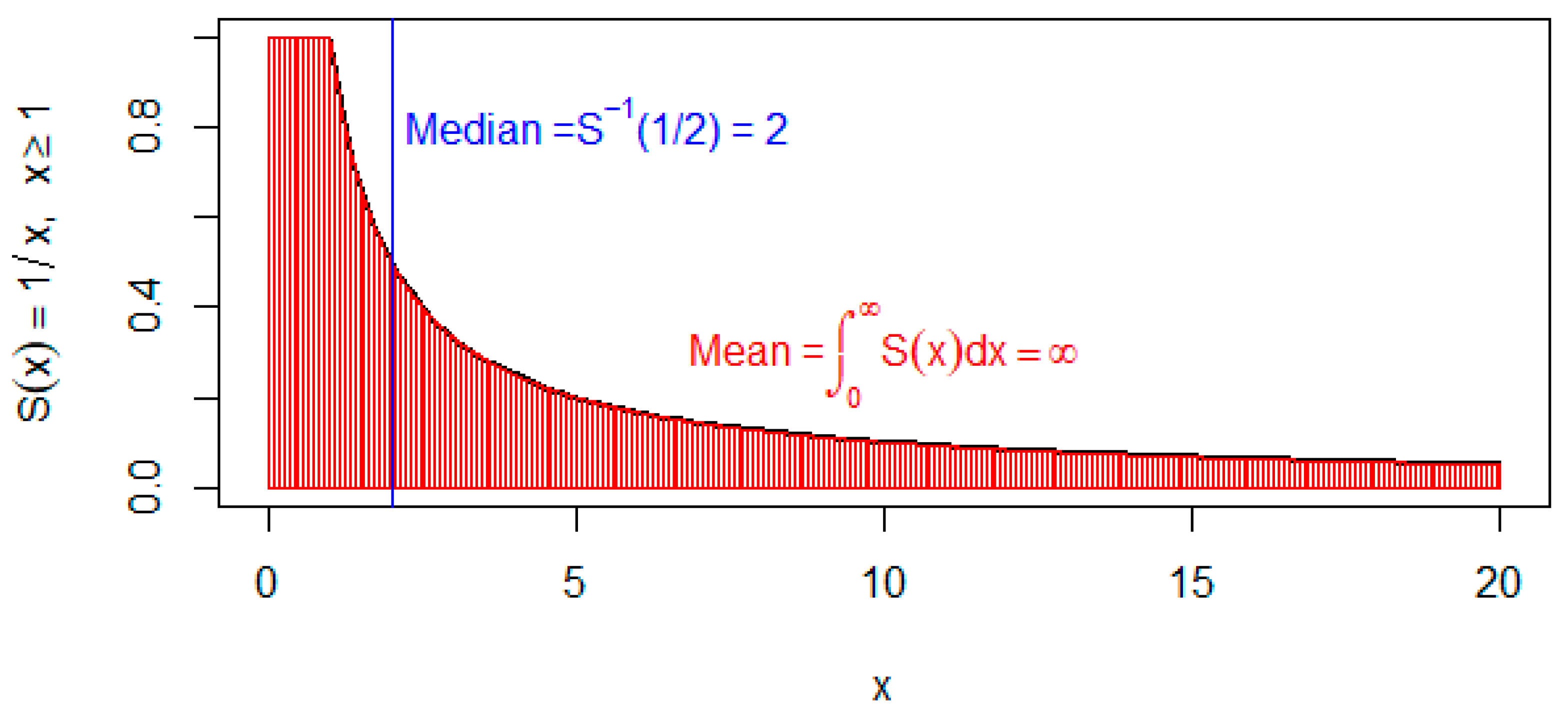
Figure 1 shows an example of a survival function, defined as

$$S\left(x\right)=\{\begin{array}{c}1 \mathrm{if} 0\le x<1,\\ 1/x \mathrm{if} x\ge 1\end{array}$$

.

We see $S\left(0\right)=1$ and $S\left(x\right)$ is decreasing toward zero as $x\to \infty$. We will see that this survival function belongs to the Pareto type I distribution (Section 3.8). The pdf is

$$f\left(x\right)=\{\begin{array}{c}0 \mathrm{if} 0\le x<1,\\ 1/x^2 \mathrm{if} x\ge 1\end{array}$$

.

It is easy to see

$$E\left(X\right)=\underset{0}{\overset{\infty }{{\displaystyle \int }}}xf\left(x\right) dt=\underset{0}{\overset{\infty }{{\displaystyle \int }}}S\left(x\right) dx=1+\underset{1}{\overset{\infty }{{\displaystyle \int }}}1/x dx={1+\ln \left(x\right)|}_1^{\infty }=\infty .$$

Thus, the mean does not exist since the area under $S\left(x\right)$ blows up to infinity (Figure 1).

The $p$-th quantile is defined by solving $F\left(x\right)=p$ with respect to $x$, and therefore, is denoted by $x_p=F^{-1}\left(p\right)=S^{-1}\left(1-p\right)$. It may also be called the $100\times p$-th percentile. The median is defined as $x_{0.5}=F^{-1}\left(0.5\right)=S^{-1}\left(0.5\right)$, which represents a “typical” life. In reliability, one often needs to control the probability of early failure via low percentiles, such as $x_{0.01}$ and $x_{0.10}$, representing 1% and 10% points, in order to meet the minimal requirement for products’ life [14,27,28]. The median is often more useful than the mean since the mean may not exist for some distributions (e.g., Pareto types I and II distributions). For instance, Figure 1 shows that the mean is infinite while the median exists.

According to Halley’s life table, the probability of survival at age 20 years is 40.8%, namely, $S\left(20\right)=0.408$ [13]. This probability decreases as the age increases, and reaches almost zero at age 85 years, namely,$S\left(85\right)\approx 0$. This is an example of survival probabilities computed by observed data. Survival probabilities can also be computed by fitting parametric distributions to observed data (Section 4).

2.3. Hazard Function

The hazard rate at time $x$ is the rate of dying at the next moment $x+\Delta x$, where $\Delta x$ is a small value. In medicine, the hazard rate is an important measure for patients’ risks. The hazard function is the most fundamental quantity in reliability analysis as well [13,14]. In addition, hazard functions are used under different names in various fields, such as the “instantaneous failure rate” in reliability engineering [14,29] and the force of mortality in demographics [30].

The hazard function (or hazard rate function) is defined as

$$h\left(x\right)=\underset{\mathsf{\Delta }x\to 0}{\lim }P\left(x\le X\langle x+\Delta x|X\ge x\right)/\Delta x$$

(1)

From Equation (1), the hazard function is derived from the survival function via

$$h\left(x\right)=-\frac{1}{S\left(x\right)}\frac{dS\left(x\right)}{dx}=-\frac{d\ln \left\{S\left(x\right)\right\}}{dx}$$

(2)

Equation (2) also means $h\left(x\right)=f\left(x\right)/S\left(x\right)$.

The cumulative hazard function is defined as $H\left(x\right)=\underset{0}{\overset{x}{{\displaystyle \int }}}h\left(u\right) du$. The cumulative hazard function and survival function are related via $H\left(x\right)=-\ln \left\{S\left(x\right)\right\}$ and $S\left(x\right)=\exp \left\{-H\left(x\right)\right\}$. Thus, the hazard function is easy to be converted to the survival function, and vice versa.

2.4. Shape of Hazard Function

The hazard function describes the dynamic change of the probability of an event over time, and hence, it exhibits a variety of shapes [5,12,14,31,32,33]. An increasing hazard function corresponds to the cases of natural aging, wear-out, and fatigue. A decreasing hazard function arises for devices with defects, such as electronic devices that are considered to have an early breakdown, or patients who undergo organ transplantation resulting in early death. This decreasing hazard during early life is said to have “infant mortality”. The hazard function of the bathtub curve is the most appropriate when both infant mortality and aging co-exist, when observing an individual over a long period of time. In the case of a manufactured item, an initial failure due to a defective part tends to occur, followed by constant hazards, and finally, the hazard increases later in the life of the equipment. Based on demographic data released by the government, in the early stages, there are many deaths, mainly due to infant mortality [5,14]. The mortality rate may then be stabilized in middle age, before increasing sharply with increasing elderly age. If the hazard function increases in the early stages and eventually starts to decrease, the hazard function has the characteristics of a hump shape. The breast cancer data example in Section 3.9 supports this shape. Accordingly, the hazard function could describe the characteristics of the failure process.

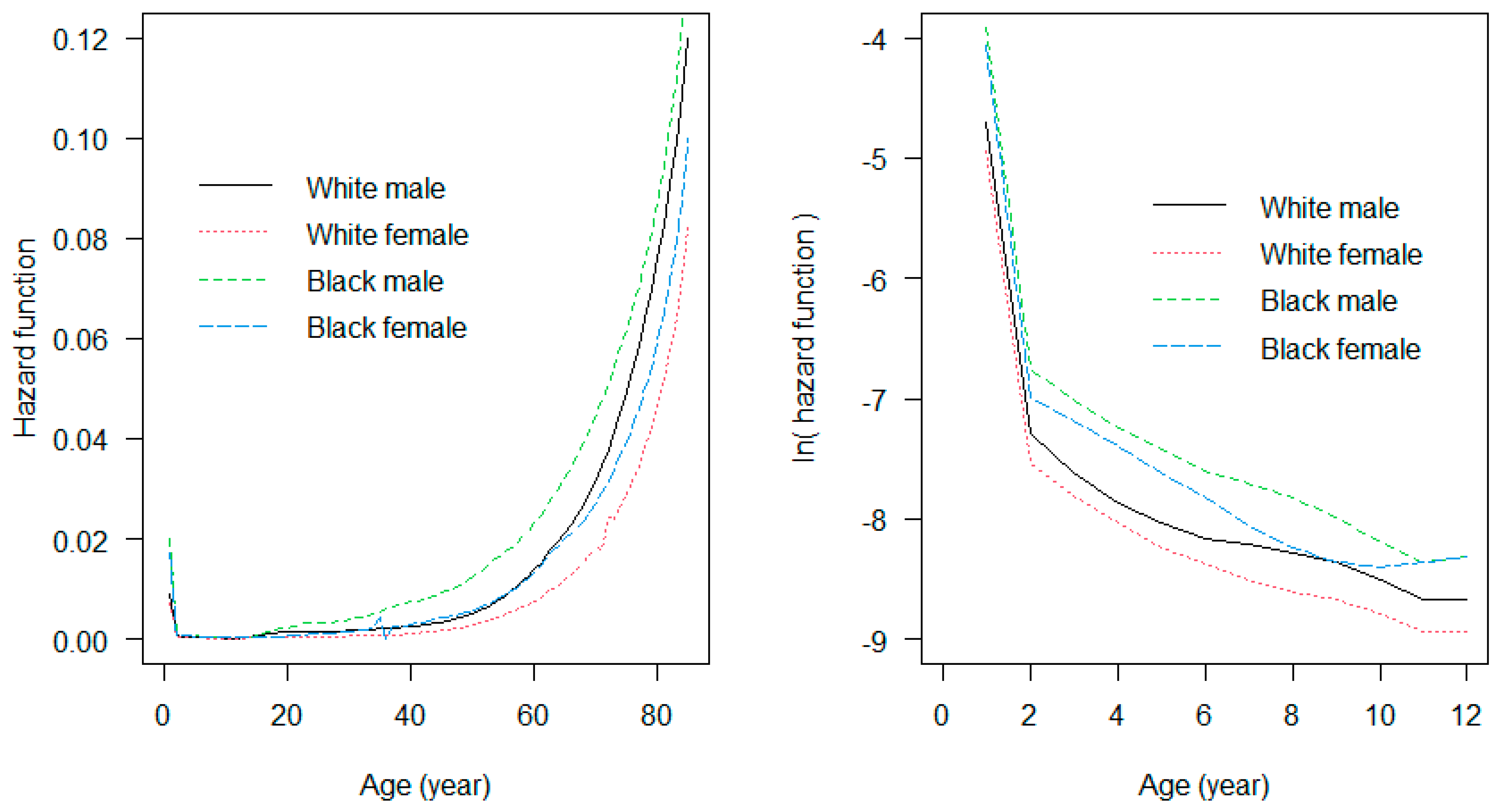
Figure 2 shows bathtub-shaped hazard functions for ages 1 to 85 estimated by the data collected from the residents of the United States as introduced by Klein and Moeschberger [5]. We see that the hazard gradually increases as they get older. However, for very young children, the hazard is somewhat high for all genders and races. Indeed, for ages 1 to 12, the hazard gradually decreases as they grow (the right panel of Figure 2).

The hazard function has visually attractive information about the underlying mechanism of death/failure. Thus, the hazard function should be considered for the interpretation of parametric models rather than the survival function. However, the survival function is usually easier to estimate by data (Section 4). The cumulative hazard function is also easy to estimate, and is often useful in acceleration tests and fatigue tests for reliability analysis of equipment because they give intuitive information about the suitability of the model [34,35]. Hence, both the hazard and survival functions play important roles in survival and reliability analyses.

3. Parametric Models

This section describes a variety of parametric distributions that are widely recognized for survival and reliability analyses.

Table 1. Parametric distributions for survival and reliability analyses.

Distribution	Parameter	Hazard Function	Survival Function	Expectation
Exponential	$\lambda >0$	$\lambda$	$\exp \left(-\lambda x\right)$	$1/\lambda$
Piecewise Exponential	${\lambda }_i>0,$ $j=1,\dots ,m$	${\displaystyle \sum }_{j=1}^m{\lambda }_j{I}_{\left(a_{j-1}, a_j\right]}\left(x\right)$	$\exp \left\{-{\lambda }_j\left(x-a_{j-1}\right)- {\displaystyle \sum }_{k=1}^{j-1}{\lambda }_k\Delta a_k\right\}, x\in \left(a_{j-1}, a_j\right]$	-
Weibull	$\alpha ,\lambda >0$	$\alpha \lambda x^{\alpha -1}$	$\exp \left(-\lambda x^{\alpha }\right)$	${\lambda }^{-1/\alpha }\mathsf{\Gamma }\left(1+1/\alpha \right)$
Rayleigh	$\lambda >0$	$2\lambda x$	$\exp \left(-\lambda x^2\right)$	${\lambda }^{-1/2}\sqrt{\pi }/2$
Gamma	$\beta ,\lambda >0$	$\frac{-dS\left(x\right)/dx}{S\left(x\right)}$	$\underset{x}{\overset{\infty }{{\displaystyle \int }}}\frac{{\lambda }^{\beta }{t}^{\beta -1}\exp \left(-\lambda t\right)}{\mathsf{\Gamma }\left(\beta \right)} dt$	$\frac{\beta }{\lambda }$
Lognormal	$\sigma >0$	$\frac{1}{S\left(x\right)\sigma x}\varphi \left(\frac{\ln x-\mu }{\sigma }\right)$	$1-\mathsf{\Phi }\left(\frac{\ln x-\mu }{\sigma }\right)$	$\exp \left(\mu +\frac{{\sigma }^2}{2}\right)$
Log-logistic	$\alpha$,$\lambda >0$	$\frac{\alpha \lambda x^{\alpha -1}}{1+\lambda x^{\alpha }}$	$\frac{1}{1+\lambda x^{\alpha }}$	${\lambda }^{-\frac{1}{\alpha }}\mathsf{\Gamma }\left(1+\frac{1}{\alpha }\right)\mathsf{\Gamma }\left(1-\frac{1}{\alpha }\right)$
Pareto I	$\alpha ,\lambda >0$	$\frac{\alpha }{x}I\left(x\ge \frac{1}{\lambda }\right)$	$\frac{1}{{\left(\lambda x\right)}^{\alpha }}I\left(x\ge \frac{1}{\lambda }\right)$	$\frac{\alpha }{\lambda \left(\alpha -1\right)}, \alpha >1$
Pareto II	$\alpha ,\lambda >0$	$\alpha \lambda /\left(1+\lambda x\right)$	${\left(1+\lambda x\right)}^{-\alpha }$	$1/\left[\lambda \left(\alpha -1\right)\right], \alpha >1$
Pareto IV	$\alpha ,\lambda >0;$ $\delta \ge 0$	$\frac{\alpha \lambda }{\delta }\frac{{\left(\lambda x\right)}^{1/\delta -1}}{1+{\left(\lambda x\right)}^{1/\delta }}$	${\left\{1+{\left(\lambda x\right)}^{\frac{1}{\delta }}\right\}}^{-\alpha }$	$\alpha {\lambda }^{-1}\mathrm{B}\left(\alpha -\delta ,1+\delta \right),$ $\alpha >\delta >0$
Hjorth	$\alpha ,\delta \ge 0;$ $\lambda >0$	$\delta x+\frac{\alpha }{1+\lambda x}$	$\frac{\exp \left(-\frac{\delta x^2}{2}\right)}{{\left(1+\lambda x\right)}^{\frac{\alpha }{\lambda }}}$	$\left(\frac{1}{\lambda }\right)\mathrm{H}\left(\frac{\delta }{{\lambda }^2},\frac{\delta }{\lambda }\right)$
Burr III	$\alpha ,\delta >0$	$\frac{-dS\left(x\right)/dx}{S\left(x\right)}$	$1-{\left(1+x^{-\delta }\right)}^{-\alpha }$	${\alpha }^{\frac{1}{\delta }}\mathrm{B}\left(1-\frac{1}{\delta },\alpha +\frac{1}{\delta }\right)$
Burr XII	$\alpha ,\delta >0$	$\frac{\alpha \delta x^{\delta -1}}{\left(1+x^{\delta }\right)}$	${\left(1+x^{\delta }\right)}^{-\alpha }$	$\alpha \mathrm{B}\left(\alpha -\frac{1}{\delta },1+\frac{1}{\delta }\right)$
Exponential power	$\alpha ,\lambda >0$	$\alpha \lambda {\left(\lambda x\right)}^{\alpha -1}{e}^{{\left(\lambda x\right)}^{\alpha }}$	$\exp \left\{1-e^{{\left(\lambda x\right)}^{\alpha }}\right\}$	-
Gompertz	$\alpha ,\lambda >0$	$\alpha \lambda e^{\lambda x}$	$\exp \left\{-\alpha \left(e^{\lambda x}-1\right)\right\}$	$\left(1/\lambda \right)\exp \left(\alpha \right)\mathrm{Ei}\left(\alpha \right)$
Generalized Gamma	$\alpha ,\beta ,\lambda >0$	$\frac{-dS\left(x\right)/dx}{S\left(x\right)}$	$\underset{x}{\overset{\infty }{{\displaystyle \int }}}\frac{\alpha {\lambda }^{\beta }{t}^{\alpha \beta -1}\exp \left(-\lambda t^{\alpha }\right)}{\mathsf{\Gamma }\left(\beta \right)} dt$	$\underset{0}{\overset{\infty }{{\displaystyle \int }}}S\left(x\right) dx$
Birnbaum–Saunders	$\beta ,\sigma >0$	$\frac{-dS\left(x\right)/dx}{S\left(x\right)}$	$\mathsf{\Phi }\left[\frac{1}{\sigma }\left({\left(\frac{x}{\beta }\right)}^{-\frac{1}{2}}-{\left(\frac{x}{\beta }\right)}^{\frac{1}{2}}\right)\right]$	$\beta \left(1+\frac{{\sigma }^2}{2}\right)$
Exponential-logarithmic	$\lambda >0;$ $0<p<1$	$\frac{-dS\left(x\right)/dx}{S\left(x\right)}$	$\frac{\ln \left[1-\left(1-p\right){\mathrm{e}}^{-\lambda x} \right]}{\ln \left(p\right)}$	$-\frac{\mathrm{polylog}\left(2,1-p\right)}{\lambda \ln \left(p\right)}$
Generalized-Exponential	$\beta ,\lambda >0$	$\left[-dS\left(x\right)/dx\right]/S\left(x\right)$	$1-{\left[1-\exp \left(-\lambda x\right)\right]}^{\beta }$	Gupta and Kundu [36]
Exponentiated-Weibull	$\beta ,\lambda ,\gamma >0$	$\left[-dS\left(x\right)/dx\right]/S\left(x\right)$	$1-{\left[1-\exp \left(-\lambda x^{\gamma }\right)\right]}^{\beta }$	Nadarajah and Gupta [37]
G-modified Weibull	$\alpha ,\beta ,\gamma ,\lambda >0$	$\left[-dS\left(x\right)/dx\right]/S\left(x\right)$	$1-{\left[1-\exp \left(-\alpha x^{\gamma }{\mathrm{e}}^{\lambda x}\right)\right]}^{\beta }$	Carrasco et al. [38]
M-spline	$h_{\ell }\ge 0,$ $\ell =1, \dots ,L$	${\displaystyle \sum }_{\ell =1}^L{h}_{\ell }{M}_{\ell }\left(x\right)$	$\exp \left\{-{\displaystyle \sum }_{\ell =1}^L{h}_{\ell }{M}_{\ell }\left(x\right)\right\}$	-

Note: The mean of the Pareto types I–II goes to infinity for $\alpha \le 1$. G-modified = Generalized modified.$I_{\left(a_{j-1}, a_j\right]}\left(x\right)=I(a_{j-1}<x\hspace{0.17em}\le a_j)$;$\Delta a_k=a_k-a_{k-1}$, $\mathrm{H}\left(a,b\right)=\underset{0}{\overset{\infty }{{\displaystyle \int }}}\exp \left(-a{t}^2/2\right)/{\left(1+t\right)}^{b}dt$; $\mathrm{B}\left(a,b\right)=\underset{0}{\overset{\infty }{{\displaystyle \int }}}{t}^{a-1}{\left(1-t\right)}^{b-1}dt$; $\mathrm{polylog}\left(2,z\right)={\displaystyle \sum }_{k=1}^{\infty }{z}^k/k^2$. $\mathrm{Ei}\left(a\right)=\underset{a}{\overset{\infty }{{\displaystyle \int }}} \exp \left(-t\right)/tdt$.

gives a list of 22 distributions selected by a procedure described in Appendix A. Many distributions have the scale parameter and shape parameter. In addition, all the distributions have the time $x$, restricted to non-negative values $x\ge 0$.

Some of the distributions have a long tail to the right, such as the Pareto distributions of types I and II. In such distributions, the value of the shape parameter causes the tail of the distribution to become very heavy, and thus, the mean may not exist. Therefore, for data in which the population follows these distributions, even if the mean or variance is calculated from the data, it does not provide useful information for the population.

In the following, the individual distributions are explained in detail.

3.1. Exponential Distribution and Its Variants

Historically, exponential distribution has been widely used in reliability engineering as a distribution of the lifetime of materials, products, and equipment. Many papers began to be published as statistical models for reliability analysis around the 1960s, when Epstein [39] started discussing estimation theory under censored data.

The survival function of the exponential distribution is $S\left(x\right)=\exp \left(-\lambda x\right), x\ge 0$. Here, $\lambda >0$ is a scale parameter (also called a rate parameter). In reliability, $\lambda$ is called “failure rate” and may be interpreted as the number of failures per million hours, percent per month, etc. This is because the hazard function is $h\left(x\right)=\lambda$. The mean and variance of $X$ following such an exponential distribution are

$$E\left(X\right)=1/\lambda , V\left(X\right)=1/{\lambda }^2.$$

A remarkable feature of the exponential distribution is the “memoryless” property, given by

$$S\left(x\right)=P\left(X\ge x|X\ge 0\right)=P\left(X\ge x+t|X\ge t\right), t>0, x>0.$$

That is, the $x$-year survival probability is equal to the $x$-year survival probability after surviving $t$ years. This property may apply to a person who stays young and is of uncertain age $t$. This property is a consequence of the constant hazard function, $h\left(x\right)=\lambda$; the risks of death are unchanged over time. The $p$-th quantile is $x_p=-\left(1/\lambda \right)\ln \left(1-p\right)$.

Many modern researchers think that the exponential distribution does not fit to real data since it has only one parameter (see Section 4 for a real data example). Since the hazard function of the exponential distribution is constant, there is a concern that it cannot explain the time transition of the hazard rate. Nelson [14] wrote, “it adequately describes only 10 to 15% of products in the lower tail of the distribution”. On the other hand, the exponential distribution has been useful for the analysis of complex survival data, such as those involving double truncation [40,41], recurrent events [42], competing risks [43], and sequential sampling designs [44], and progressive censoring [45]. The analysis of such complex survival data is made possible by the simplicity of the exponential distribution.

The exponential distribution is the basis of creating many distributions: by adding one parameter, the Weibull and gamma distributions can be obtained. The exponential power distribution (Table 1) is a distribution that can model bathtub-type hazard functions [46], which is useful for reliability analysis. The piecewise exponential model (Table 1) is defined as $h\left(x\right)={\lambda }_j$ for $x\in \left(a_{j-1},a_j\right]$, $j=1,\dots ,m$, defined on a prespecified knot sequence $0=a_0<a_1<\dots <a_m$, and $m$ is the number of pieces. The piecewise exponential distribution has been successfully adapted for modeling event times for biological, medical, environmental, and econometric studies [25,47,48,49,50,51].

3.2. Weibull Distribution

The Weibull distribution was first proposed by Rosin and Rammler [52] who applied it to describe the law governing the fineness of pulverized coal (it is also known as the Rosin–Ramler distribution). Later, Werody Weibull [53,54] proposed a distribution for the lifespan of materials. This distribution has been used to analyze a lot of lifetime data, including human subjects, such as the death time of Hiroshima’s atomic bomb survivors [55].

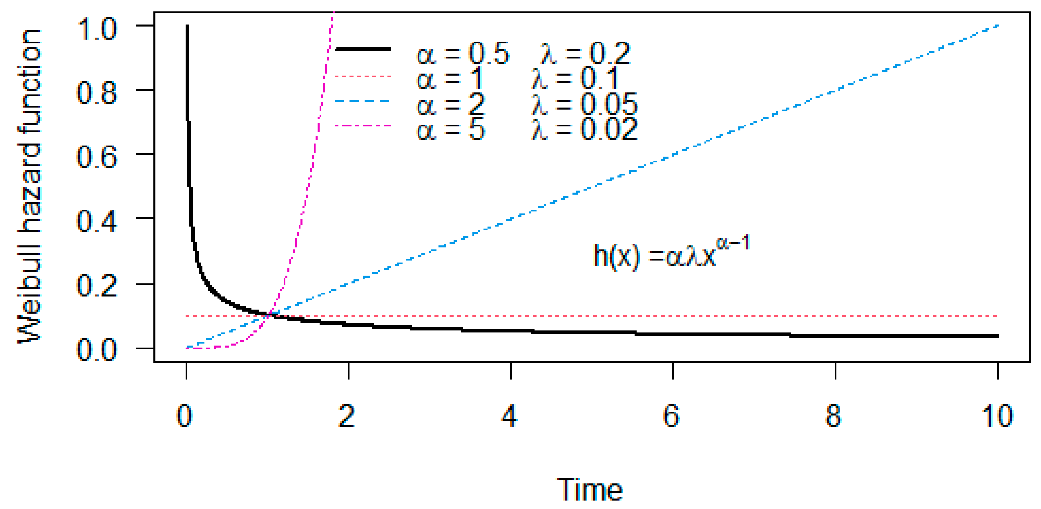
The Weibull survival function is $S\left(x\right)=\exp \left(-\lambda x^{\alpha }\right), x\ge 0$, with the scale parameter $\lambda >0,$ and the shape parameter $\alpha >0$. The case of $\alpha =1$ reduces to the exponential distribution having a constant hazard function $h\left(x\right)=\lambda$. The case of $\alpha =2$ gives the Rayleigh distribution (named after Lord Rayleigh) having a linear hazard function $h\left(x\right)=2\lambda x$. Thus, the Weibull distribution is more flexible than the exponential and Rayleigh distributions. Figure 3 shows the hazard functions with the increasing ($\alpha >1$), constant ($\alpha =1$), and decreasing ($\alpha <1$) shapes.

The Weibull distribution is useful because the survival and hazard functions are simple, and the shape parameters is easy to interpret. Furthermore, the formula of the moments of a random variable $X$ following such a Weibull distribution is

$$E\left(X^r\right)={\lambda }^{-r/\alpha }\mathsf{\Gamma }\left(1+r/\alpha \right), r>-\alpha ,$$

where $\mathsf{\Gamma }\left(\alpha \right)=\underset{0}{\overset{\infty }{{\displaystyle \int }}}{u}^{\alpha -1}{e}^{-u} du$ is the gamma function for $\alpha >0$. The mean and variance are,

$$E\left(X\right)={\lambda }^{-1/\alpha }\mathsf{\Gamma }\left(1+1/\alpha \right),$$

$$V\left(X\right)={\lambda }^{-2/\alpha }\left[\mathsf{\Gamma }\left(1+2/\alpha \right)-\mathsf{\Gamma }{\left(1+1/\alpha \right)}^2\right].$$

The $p$-th quantile is $x_p={\left[-\left(1/\lambda \right)\ln \left(1-p\right)\right]}^{1/\alpha }$.

Let $Y=\ln \left(X\right)$, where $X$ follows the Weibull distribution. Then,

$$P\left(Y>y\right)=\exp \left[-\exp \left(\frac{y-\mu }{\sigma }\right)\right]=S_0\left(\frac{y-\mu }{\sigma }\right), -\infty <y<\infty .$$

where $\mu =-{\alpha }^{-1}\ln \left(\lambda \right)$, $\sigma ={\alpha }^{-1}$, and $S_0\left(w\right)=\exp \left(-e^w\right)$, $-\infty <w<\infty$. Thus, one can write $Y=\mu +\sigma W$, where $W$ has the standard extreme value distribution with $P\left(W>w\right)=S_0\left(w\right)$. Thus, $Y$ follows the extreme value distribution with the location parameter $\mu$ and scale parameter $\sigma$ [4,5,12].

A number of papers adopted the Weibull distribution for accelerated life data [27,56,57,58,59], left-truncated data [60,61], breast/colorectal/ovarian cancer data [6,62,63,64], the AIDS data [65], and others. The Weibull distribution is also useful for creating multivariate survival distributions [66]. Some authors employed the Weibull distribution as a convenient choice for multivariate survival and competing risk models under the common shape parameter [67,68,69].

3.3. Lognormal Distribution

The lognormal distribution is perhaps the third most popular distribution after the exponential and Weibull distributions. The lognormal distribution has a good ability to fit data for reliability analysis, such as the analysis of equipment failure time under fatigue life testing [35,70] or under field reliability testing [71,72,73,74]. The reason for its popularity is its relationship with normal distribution. However, the lognormal distribution exhibits surprisingly good fits to many data with no particular relationship with the normal distribution [75].

Let $N\left(\mu ,{\sigma }^2\right)$ denote a normal distribution with mean $\mu$ and variance ${\sigma }^2$.

A random variable $X$ follows the lognormal distribution if $\ln \left(X\right)$ follows $N\left(\mu ,{\sigma }^2\right)$. The pdf of the lognormal distribution is

$$f\left(x\right)=\frac{1}{x\sigma \sqrt{2\pi }}\exp \left\{-\frac{1}{2}{\left(\frac{\ln x-\mu }{\sigma }\right)}^2\right\}=\frac{1}{x\sigma }\varphi \left(\frac{\ln x-\mu }{\sigma }\right),x>0,$$

where $\varphi \left(z\right)=\left(1/\sqrt{2\pi }\right)\exp \left(-z^2/2\right)$ is the pdf of $N\left(0,1\right)$. The survival function is

$$S\left(x\right)=P\left(X>x\right)=1-\mathsf{\Phi }\left(\frac{\ln x-\mu }{\sigma }\right),x>0,$$

where $\mathsf{\Phi }\left(z\right)=\underset{-\infty }{\overset{z}{{\displaystyle \int }}}\varphi \left(w\right)dw$ is the cumulative distribution function of $N\left(0,1\right)$. The mean and variance of the lognormal distribution are, respectively,

$$E\left(X\right)=\exp \left(\mu +\frac{{\sigma }^2}{2}\right), V\left(X\right)=\left\{\exp \left({\sigma }^2\right)-1\right\}\exp \left(2\mu +{\sigma }^2\right).$$

The hazard function of the lognormal distribution is

$$h\left(x\right)=\frac{ 1}{x\sigma }\frac{\varphi \left(\frac{\ln x-\mu }{\sigma }\right)}{\left\{1-\mathsf{\Phi }\left(\frac{\ln x-\mu }{\sigma }\right)\right\}}, x>0.$$

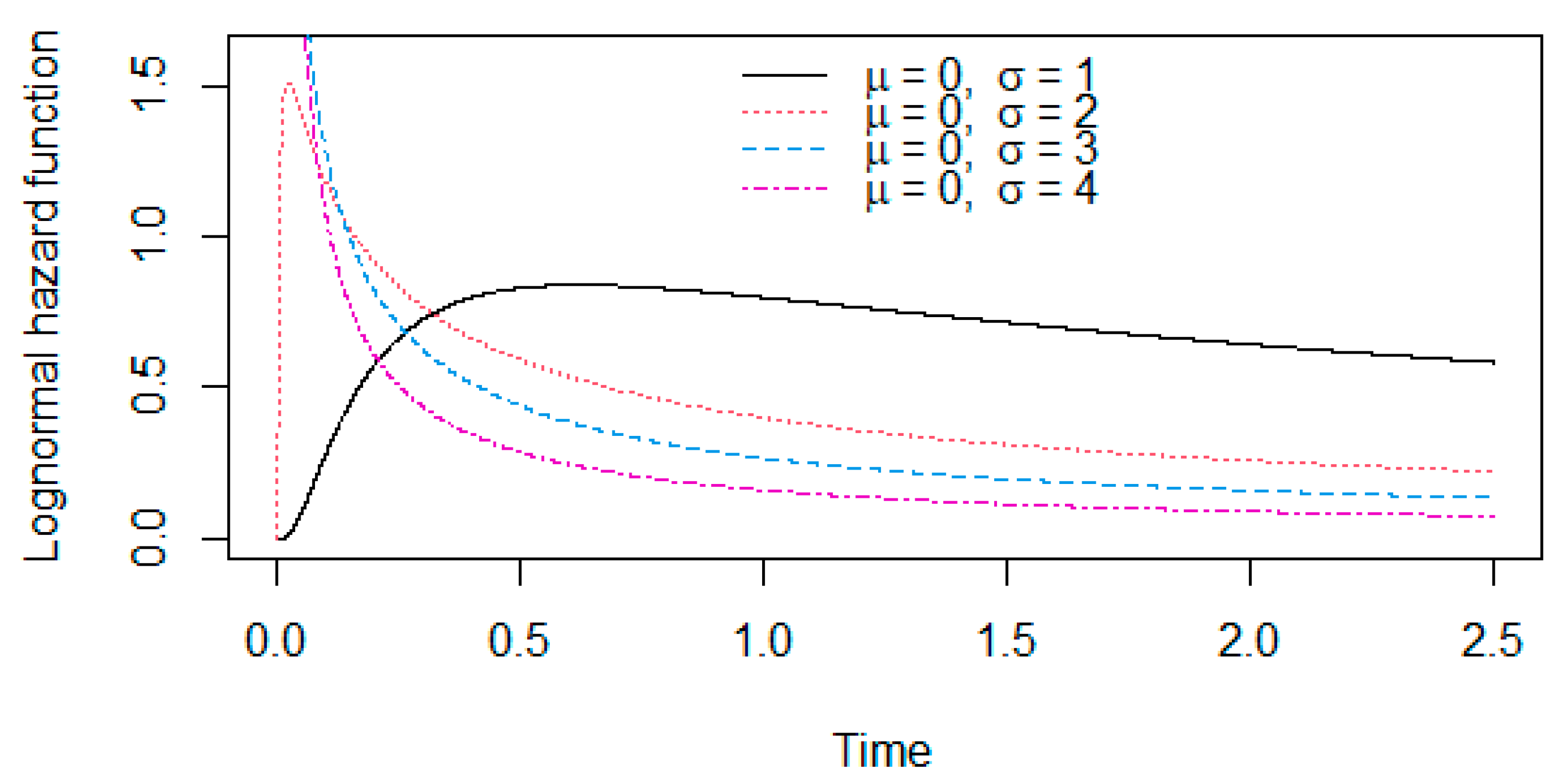
In this model, the hazard function at $x=0$ is ${\lim }_{x\to +0}h\left(x\right)=0$. Figure 4 shows that $h\left(x\right)$ is a one-hump shape. In many human and mechanical individuals, it is assumed that the hazard increases as they get old. Since the hazard function of the lognormal distribution does not allow this aging process, it has been criticized as unrealistic in many situations.

If $X$ follows the lognormal distribution, one can write $\ln X=\mu +\sigma W$, where $W$ follows the standard normal $N\left(0,1\right)$ distribution.

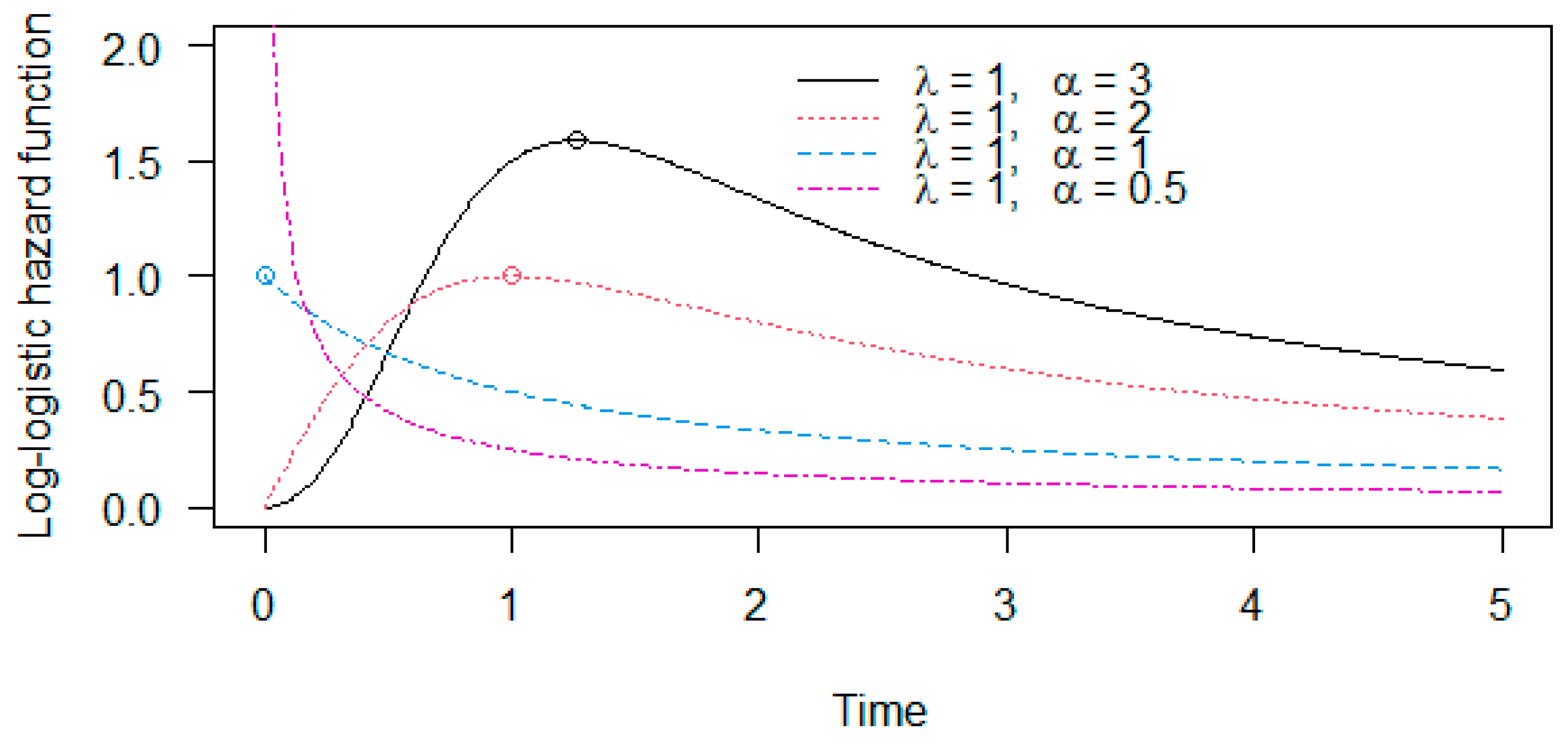
3.4. Log-Logistic Distribution

We have seen that the three most popular distributions (exponential, Weibull, and lognormal) are all written as $\ln \left(X\right)=\mu +\sigma W$, where $W$ follows some standard distribution. If one assumes that $W$ follows the standard logistic distribution,$P\left(W>w\right)=1/\left\{1+\exp \left(w\right)\right\}$, $-\infty <w<\infty$, then, $X$ yields the log-logistic distribution.

A random variable $X$ follows the log-logistic distribution if $\ln \left(X\right)$ follows a logistic distribution with the location parameter $\mu$ and the scale parameter $\sigma$, defined as

$$P\left(\ln \left(X\right)>y\right)=\frac{1}{1+\exp \left(\frac{y-\mu }{\sigma }\right)} , -\infty <y<\infty ,$$

Re-parameterizing by $\alpha =1/\sigma$ and $\lambda =\exp \left(-\mu /\sigma \right)$, the survival function of $X$ is

$$S\left(x\right)=P\left(X>x\right)=\frac{1}{1+\lambda x^{\alpha }}, x>0.$$

Here, we call $\lambda >0$ scale parameter, and $\alpha >0$ shape parameter.

Since the logistic function $\exp \left(z\right)/\left[1+\exp \left(z\right)\right]$ and the probit function $\mathsf{\Phi } \left(z\right)$ are similar in shape, the log-logistic distribution is similar to the lognormal distribution. Nonetheless, it is possible to distinguish two distributions from the data [76].

The hazard function is

$$h\left(x\right)=\frac{\alpha \lambda x^{\alpha -1}}{\left(1+\lambda x^{\alpha }\right)}, x>0.$$

The numerator of the hazard function is the same as that of the Weibull distribution. However, the shape of the hazard function is rather similar to that for the lognormal distribution (compare Figure 4 and Figure 5 side by side). The hazard function is either decreasing ($\alpha \le 1$) or hump-shaped ($\alpha >1$) with the mode ${\left\{\left(\alpha -1\right)/\lambda \right\}}^{1/\alpha }$ for $\alpha \ge 1$ (see the circles in Figure 5).

The $p$-th quantile is $x_p={\left[{\lambda }^{-1}p/\left(1-p\right)\right]}^{1/\alpha }.$ The mean and variance are, respectively,

$$E\left(X\right)={\lambda }^{-\frac{1}{\alpha }}\mathsf{\Gamma }\left(1+\frac{1}{\alpha }\right)\mathsf{\Gamma }\left(1-\frac{1}{\alpha }\right) , \alpha >1$$

$$V\left(X\right)={\lambda }^{-\frac{2}{\alpha }}\left[\mathsf{\Gamma }\left(1+\frac{2}{\alpha }\right)\mathsf{\Gamma }\left(1-\frac{2}{\alpha }\right)-{\mathsf{\Gamma }}^2\left(1+\frac{1}{\alpha }\right){\mathsf{\Gamma }}^2\left(1-\frac{1}{\alpha }\right)\right], \alpha >2.$$

The log-logistic, lognormal, and Weibull distributions are the three most popular members in the log-location-scale model, which are applied widely in medical studies [5,6] and engineering studies [12,13,14,15,27,73].

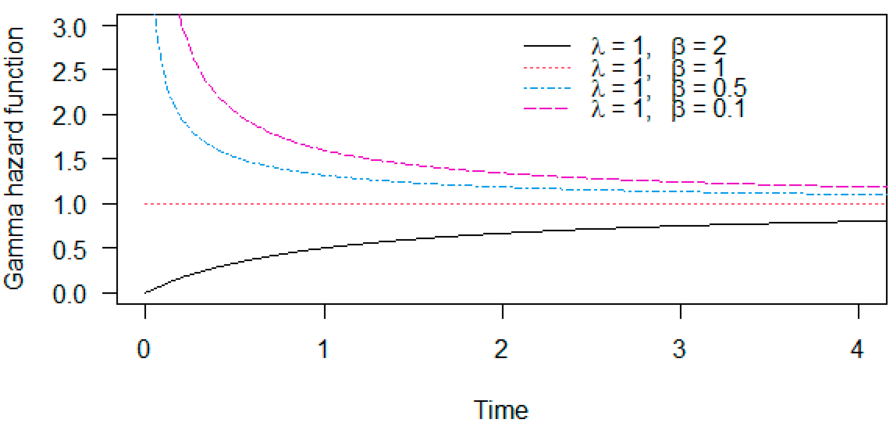
3.5. Gamma Distribution

The gamma distribution is popular in statistics. In survival and reliability analyses, it is somewhat inconvenient because the hazard function is complex. Indeed, the gamma distribution is the secondary choice to the Weibull, lognormal, and logistic distributions. In applications, the gamma distribution is applied with the lognormal and Weibull distributions [72,74,77] or without any other [78,79].

When a random variable, $X,$ follows a gamma distribution, its pdf is

$$f\left(x\right)=\frac{{\lambda }^{\beta }}{\mathsf{\Gamma }\left(\beta \right)}{x}^{\beta -1}\exp \left(-\lambda x\right), x>0,$$

for the scale parameter $\lambda >0$ and shape parameter $\beta \ge 1$. The gamma distribution includes the exponential distribution ($\beta =1$). By $\beta =v/2$ and $\lambda =1/2$, the gamma distribution includes the chi-square distribution with degrees of freedom $v$. The survival function is

$$S\left(x\right)=\frac{1}{\mathsf{\Gamma }\left(\beta \right)}\underset{x}{\overset{\infty }{{\displaystyle \int }}}\lambda {\left(\lambda t\right)}^{\beta -1}\exp \left(-\lambda t\right) dt.$$

The mean and variance of $X$ are, respectively,

$$E\left(X\right)=\beta /\lambda ,V\left(X\right)=\beta /{\lambda }^2.$$

For $\beta >1$, the hazard function is increasing, and

$$\underset{x\to +0}{\lim }h\left(x\right)=0, \underset{x\to \infty }{\lim }h\left(x\right)=\lambda .$$

For $\beta <1$, the hazard function in decreasing, and

$$\underset{x\to +0}{\lim }h\left(x\right)=\infty ,\underset{x\to \infty }{\lim }h\left(x\right)=\lambda .$$

For $\beta =1$, the hazard function is constant. Figure 6 demonstrates the above properties.

3.6. Generalized Gamma Distribution

The generalized gamma distribution is a three-parameter distribution adding one more shape parameter ($\alpha >0$) to the gamma distribution. The pdf of the generalized gamma distribution is

$$f\left(x\right)=\frac{\alpha {\lambda }^{\beta }}{\mathsf{\Gamma }\left(\beta \right)}{x}^{\alpha \beta -1}\exp \left(-\lambda x^{\alpha }\right), x>0.$$

The value $\alpha =1$ results in the gamma distribution. The value $\beta =1$ results in the Weibull distribution. The distribution was first proposed by Stacy [80]. The parameter estimation problem was considered by Stacy and Mihram [81]. The generalized gamma distribution includes the half-normal, circular normal, spherical normal, and Rayleigh distributions as special cases [81]. While the generalized gamma distribution is a flexible distribution due to the three parameters, it may produce computational problems for maximum likelihood estimation [82].

Farewell and Prentice [83] developed an alternative version of the generalized gamma distribution by including the lognormal distribution as a limiting case. This version has also been popular in reliability [15] and biostatistics [5,84,85].

3.7. Burr Distributions

Burr [86] proposed a list of twelve distributions. They are now called the Burr distribution of type I, type II, and so on. The Burr distribution of type I (the Burr I distribution) is the uniform distribution, which is less common in lifetime modeling. Among all the distributions, the Burr XII distribution is the most common and useful distribution for lifetime data analyses, and the Burr distribution usually refers to the Burr XII distribution. The Burr III distribution is also popular and often studied together with the Burr XII distribution [87,88]. We, therefore, introduce the Burr III and Burr XII distributions below.

The survival function of the Burr XII distribution is

$$S\left(x\right)={\left\{1+{\left(\lambda x\right)}^{\delta }\right\}}^{-\alpha }, x>0,$$

where $\delta >0$ and $\alpha >0$ are shape parameters. The original version is the case of $\lambda =1$ [86]. The case of $\alpha =1$ is the log-logistic distribution (Table 1). The case of $\delta =1$ is the Pareto type II (Lomax) distribution (Table 1).

The Burr XII distribution has been the basis of generating many lifetime distributions, such as the beta Burr XII distribution [89] and the Sine Burr distribution [90]. The Burr XII distribution has been applied to a number of applications, such as the multicomponent stress–strength reliability [91] and disease data analysis with competing risks [92,93].

The survival function of the Burr III distribution is

$$S\left(x\right)=1-{\left\{1+{\left(\lambda x\right)}^{-\delta }\right\}}^{-\alpha }, x>0,$$

where $\delta >0$ and $\alpha >0$ are shape parameters. The original version is the case of $\lambda =1$ (Burr [86]; Table 1). The Burr III distribution is also known as the Dagum distribution (Dagum [94]) whose properties have been investigated [95,96,97]. The Burr III distribution is the reciprocal of the Burr XII distribution. The Burr III distribution can cover a wider range of skewness and kurtosis values than the Weibull distribution does, and hence, the former can fit better than the latter in some applications [88]. The Burr III distribution has a simple distribution function $F\left(x\right)={\left(1+{\left(\lambda x\right)}^{-\delta }\right)}^{-\alpha }$. This makes the Burr III distribution useful for dealing with the stress–strength models [98,99] and latent failure time distribution for competing risk models [100,101], and bivariate distribution function [102].

3.8. Pareto Distributions

There are four types of the Pareto distribution (Pareto types I-IV distributions). Due to their popularity, we review the Pareto types I, II, and IV distributions below.

The original Pareto distribution, also known as the Pareto type I distribution (Table 1), was proposed by Vilfredo Pareto for income data. The survival function is $S\left(x\right)={\left(\lambda x\right)}^{-\alpha }I\left(x\ge 1/\lambda \right)$, where $\alpha >0$ is the shape parameter (sometimes called the Paretian index), $I(.)$ is the indicator function, and $\lambda$ is the scale parameter. Under the Pareto type I distribution, survival time $X$ takes values greater than $1/\lambda$. The hazard function is $h\left(x\right)=\left(\alpha /x\right)I\left(x\ge 1/\lambda \right)$, which is restricted to be the decreasing shape. This decreasing nature of the hazard function comprises the main feature of the Pareto type I distribution; it produces a right-skewed distribution. The Pareto type I distribution remains a useful model to fit income data and analyze their inequality [103]. The Pareto type I distribution also fits well to censored survival data from medicine [104,105] and engineering [106].

The Pareto type II distribution, also known as the Lomax distribution [107], is defined by the survival function $S\left(x\right)={\left(1+\lambda x\right)}^{-\alpha }$. The Pareto type II distribution can fit various types of data. For instance, it was chosen as the better distribution [108] than the Weibull and Gomperz distributions for the life of electric power transformers. The Pareto type IV distribution generalizes the Pareto type II by adding one more shape parameter $\delta$, leading to $S\left(x\right)={\left(1+{\left(\lambda x\right)}^{1/\delta }\right)}^{-\alpha }$. This is essentially equal to the Burr XII distribution.

We specifically notice the mathematical convenience of the Pareto II distribution in bivariate failure time data. Lindley and Singpurwalla [109] introduced a bivariate Pareto model for the life lengths of system components, which is called the Lindley-Singpurwalla bivariate Pareto (LSBP) model. Sankaran and Nair [110] extended the LSBP model for applications to reliability which shall be called the Sankaran and Nair bivariate Pareto (SNBP) model. It was also used in dynamic reliability prediction analyses [111]. Escarela and Carrière [92] proposed to fit the Frank copula model with the Pareto type II margins for the prostate cancer data. Sankaran and Kundu [112] proposed to fit the SNBP model for the life test data on appliances. See also Shih et al. [113] for the Frank copula and SNBP distributions. While these bivariate models are all based on the Pareto type II distribution, the bivariate model based on the Pareto type I distribution is referred to p.91 of Mardia [114] and Lin et al. [105].

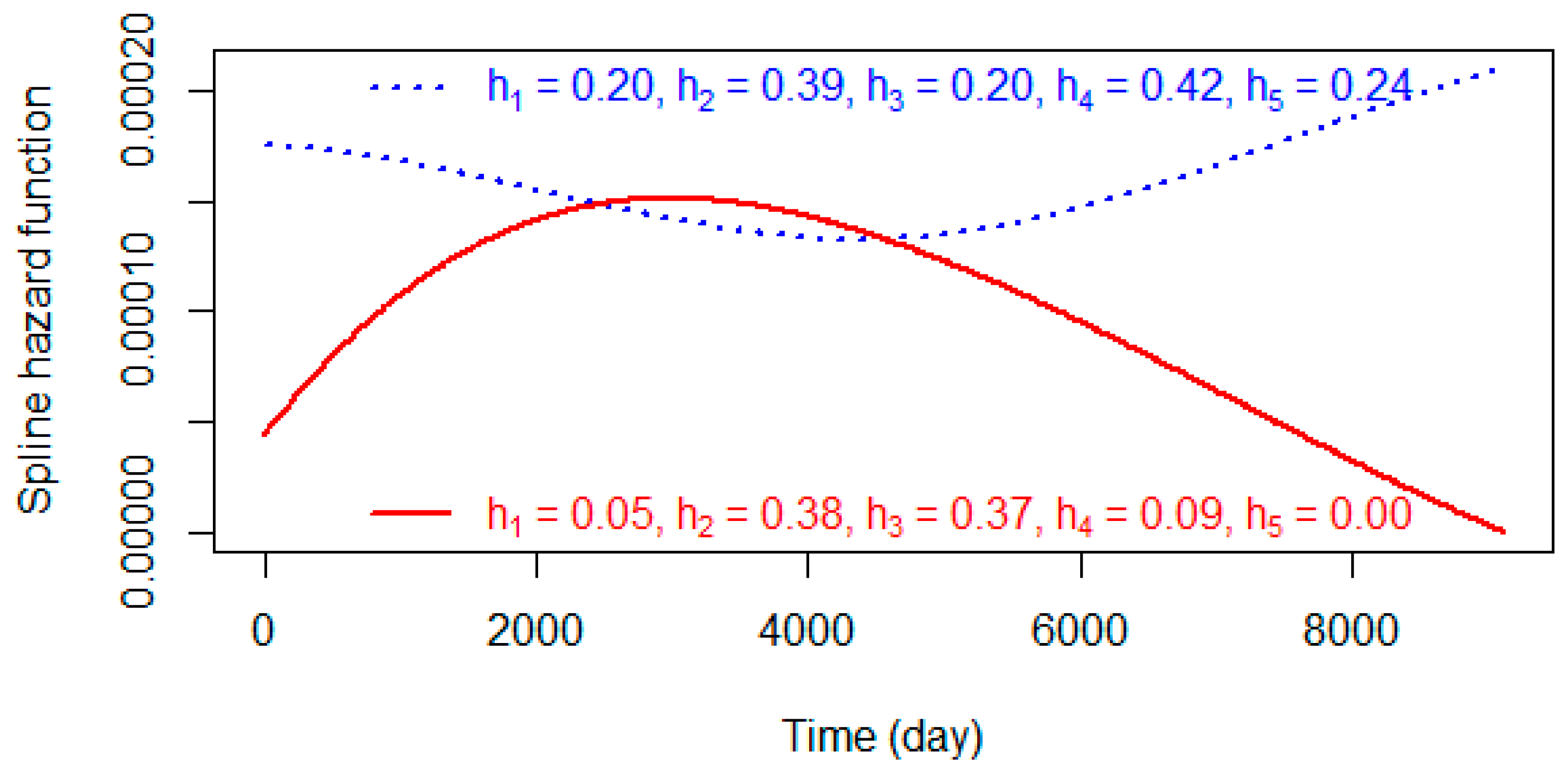
3.9. Spline Distributions

A hazard function specified by splines is more flexible than the aforementioned parametric models. A spline-based hazard function is $h\left(x\right)={\displaystyle \sum }_{\ell =1}^L{h}_{\ell }{M}_{\ell }\left(x\right)$, where $M_{\ell }\left(x\right)$ is a known basis function, and $h_{\ell }\ge 0$ is a parameter for $\ell =1, 2, \dots , L$. To define the basis functions, cubic polynomial functions are usually employed; see P.32 of Lawless [12]. Lower degrees of polynomials may also be used, such as linear and quadratic functions [115]. The books [7,12] review the spline-based methods.

The idea of modeling the hazard function via B-splines basis functions was first proposed by Klotz [115]. Inference methods for the spline-based models were further developed by Jarjoura [116] and O’Sullivan [117] via penalized likelihood procedures. In survival analysis, the B-splines may be replaced by the M-splines [118]. The M-splines are simply the standardized versions of the B-splines so that the integration becomes one.

While the spline is usually regarded as a nonparametric model, it may be treated as a parametric distribution when the number of parameters is fixed [32,115,119]. For example, for a five-parameter spline, one defines the hazard function as $h\left(x\right)={\displaystyle \sum }_{\ell =1}^5{h}_{\ell }{M}_{\ell }\left(x\right)$, where the base function $M_{\ell }\left(x\right)$ is a M-spline basis function (defined in Appendix B) for $\ell =1, 2, \dots , 5$. As in the piecewise exponential distribution, there exists a knot sequence defining the range of $x$, which is suppressed in the function $M_{\ell }\left(x\right)$. Shih and Emura [32] gave the formulas of $M_{\ell }\left(x\right)$, and showed the necessary and sufficient conditions for the parameters corresponding to the constant, increasing, decreasing, convex, and concave functions. For example, the necessary and sufficient conditions for being convex are

$$4h_1-3h_2+h_3\le 0, h_2-2h_3+h_4\le 0, h_3-3h_4+4h_5\le 0.$$

Another important feature of the spline function is that the integral of the cubic spline is explicitly available. This means that the cumulative hazard and the survival functions can be obtained explicitly via $H\left(x\right)={\displaystyle \sum }_{\ell =1}^L{h}_{\ell }{I}_{\ell }\left(x\right)$, where $I_{\ell }\left(t\right)=\underset{-\infty }{\overset{x}{{\displaystyle \int }}}{M}_{\ell }\left(t\right)dt$ is called the I-spline (the formulas are given in Appendix B). This made the spline function attractive to model marginal survival functions in copula models [9,119,120,121,122].

Figure 7 shows two hazard functions that were fitted to breast cancer patients: the time from surgery to distant metastasis (blue dotted line) and the time until death (solid red line) [122]. From the figure, the hazard function of death has the characteristics of a hump-type, and the hazard at the time of surgery is low. Just after surgery, the hazard ratio suddenly increases due to the possibility of infection, bleeding, and other complications. After some time, the hazard decreases as the patient recovers.

3.10. Other Distributions

Table 1 shows many distributions that are highly cited in the literature and widely applied to survival and reliability. Due to the space limitation, we only give the original references and some latest references for them for further reading.

The Birnbaum–Saunders distribution (Table 1) was introduced for modeling failure caused by fatigue or crack [123]. The distribution is commonly used to describe the fatigue life of metals (e.g., aluminum coupons) [123,124]. Since its original paper, the distribution has attracted a large number of statisticians for its inference methods [125,126,127].

The Hjorth distribution ([128], Table 1) is a three-parameter distribution whose hazard function is $\lambda \left(x\right)=\delta x+\alpha /\left(1+\lambda x\right)$. It can be increasing, decreasing, constant, or bathtub-shaped. The Hjorth distribution includes the Pareto type II distribution (Table 1) by $\delta =0$, and the Rayleigh distribution (Table 1) by $\alpha =0$ as a special case. One of the most recent applications is the reliability modeling of Demirci et al. [129].

The exponentiated Weibull (EW) distribution was created by adding one parameter to the Weibull distribution ([130], Table 1), and applied to the bus-motor-failure data. Gupta and Kundu [36] called it the generalized exponential distribution for the case of the exponentiated exponential distribution. Nadarajah and Gupta [37] obtained the moments of the EW distribution in a complex form. Carrasco et al. [38] proposed a generalized modified Weibull distribution (Table 1) that includes the EW distribution as a special case. This distribution has a wide range of applications (e.g., reliability applications [131]).

The exponential-logarithmic (EL) distribution was proposed by Tahmasbi and Rezaei ([132], Table 1). The EL distribution can only produce a decreasing hazard function. For this reason, some authors tried to extend this distribution to be more flexible; see the recent review and generalization by Chesneau et al. [133]. The EL distribution was derived as the minimum of N exponentially distributed random variables, where N follows the discrete logistic distribution. Thus, the EL distribution can model the lifetime of a series system consisting of N components.

4. Data Analysis

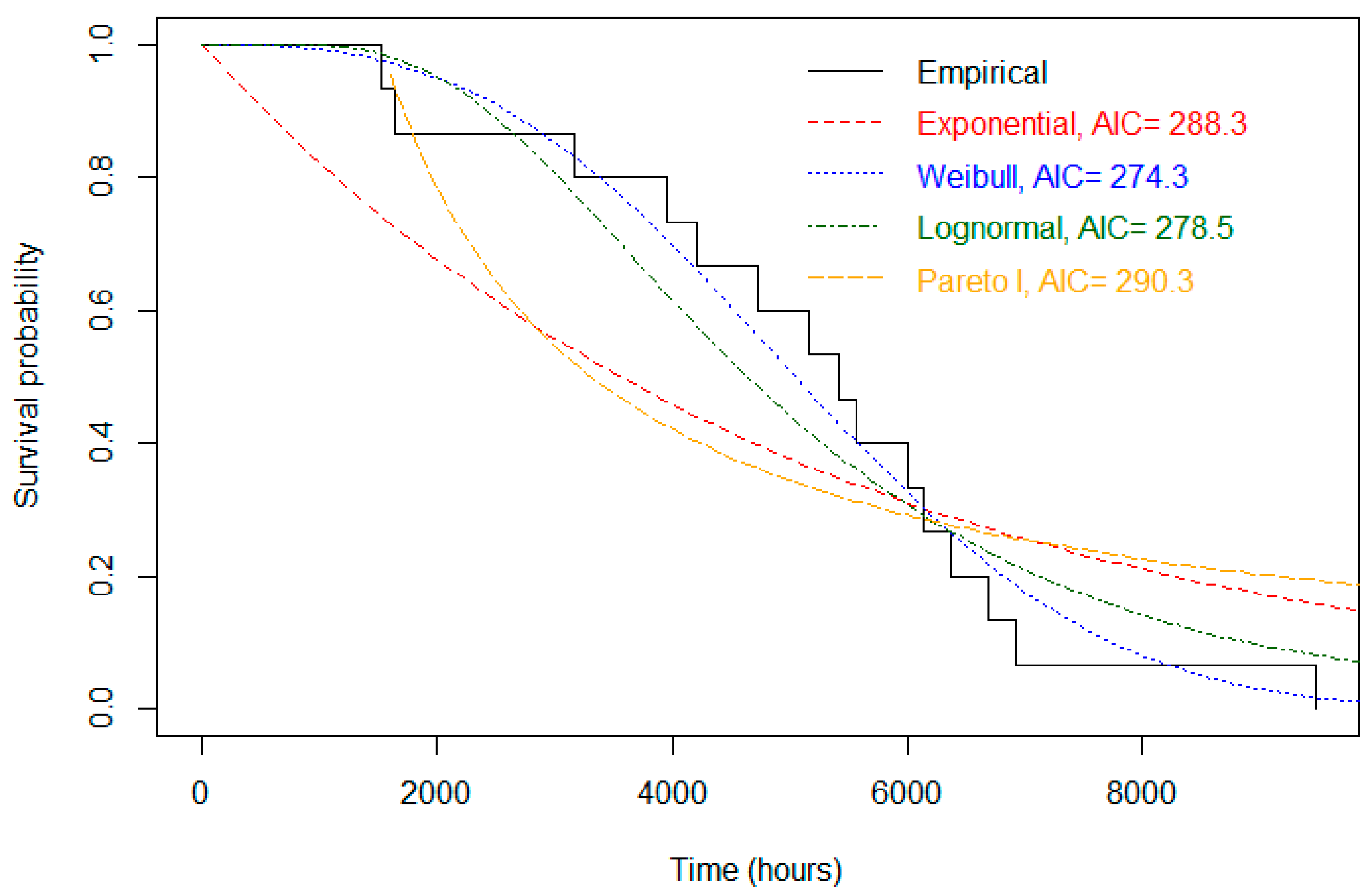
This section analyzes a real dataset to explain the ability of parametric distributions. Unless there is a prescription to choose a distribution, we suggest fitting a couple of distributions (from Table 1) and choosing one that most closely agrees with the given data.

A reliable metric for the agreement between a dataset and distribution is the Akaike Information Criterion (AIC) (Akaike [134]). The AIC is defined as −2ln(L)+2k, where L is the likelihood and k is the number of parameters. The possible formulas of ln(L) depend on the types of data (complete, right-censored, left-truncated, and others) and the distribution. A smaller value of AIC corresponds to a better model (higher likelihood and fewer parameters). The AIC can be employed when researchers try to find the best model among candidate models, as seen in Emura and Shiu [71], Korkmaz et al. [135], Santoro et al. [136], Thach [33], and others.

We consider a dataset consisting of failure times (in hours) of transmission on $n=15$ caterpillar tractors. The dataset extracted from Nayak [137] is given as follows:

{1641, 5556, 5421, 3168, 1534, 6367, 9460, 6679, 6142, 5995, 3953, 6922, 4210, 5161, 4732}.

We fitted the exponential, Weibull, lognormal, and Pareto type I distributions in order to show the different shapes of the survival functions. The parameters in all the distributions were estimated by maximizing the likelihood function $\ln \left(L\right)=\ln \left[{\displaystyle \prod }_{i=1}^{n}f\left(x_i\right)\right]$ for $n=15$ based on the formulas in Appendix C.

Figure 8 displays the empirical survival function $S\left(x\right)={\displaystyle \sum }_{i=1}^{n}I(x_i>x)/n$ and the four fitted survival functions. The values of the AIC are also shown (a smaller AIC value gives a better model). The Weibull distribution was the best model due to its smallest AIC value. Indeed, the Weibull distribution gave the survival function closest to the empirical survival function. On the other hand, the Pareto type I distribution led to the worst fit. Overall, the values of the AIC are in good agreement with the visual impressions of the goodness-of-fit of the distributions.

5. Conclusions

This paper reviews important parametric distributions used to model survival and reliability data, which consists of a list of 22 distributions (Table 1). The list could be insufficient since the research fields of survival and reliability analyses are wide-ranging, highly developed, and even growing recently [138,139,140]. Nonetheless, we hope that the list of parametric distributions may help researchers grasp the state-of-the-art knowledge for survival and reliability analyses.

We analyze a real dataset to explain how to choose a suitable model for a given data. We suggest the AIC in Section 4, yet there could be many other metrics, such as the BIC. Another commonly used metric is the Kolmogorov–Smirnov (K–S) distance defined as the sup-norm between the empirical distribution function and a fitted parametric distribution. The advantage of the K–S distance is the availability of the P-value for testing the distribution. However, the K–S distance does not account for the number of parameters, and thus, it favors a distribution with a larger number of parameters.

In practice, survival/reliability data contain covariates or acceleration factors so that regression models have to be considered [5,6,7,9,13,14,15,16]. The review of parametric regression models in survival and reliability is a potential topic for further investigation. Moreover, many real data include multivariate survival outcomes, recurrent events, dependent censoring, and competing risks [5,6,8,9,44,49,50,61,121,141,142,143,144,145]. The state-of-the art review of multivariate survival distributions and competing risk models is an important topic for further investigation.

References

- Halley, E. An estimate of the degrees of the mortality of mankind, drawn from curious tables of the births and funerals at the city of Breslaw; with an attempt to ascertain the price of annuities upon lives. Phil. Trans. R. Soc. London 1693, 17, 596–610. [Google Scholar] [CrossRef] [Green Version]
- Bellhouse, D.R. A new look at Halley’s life table. J. R. Stat. Soc. Ser. A 2011, 174, 823–832. [Google Scholar] [CrossRef]
- Bernoulli, D. Essai d’une Nouvelle Analyse de la Mortalite Cause e par la Petite Verole, et des Avantages de L’inoculation pour le Prevenir; Histoire avec le Memoires; Academie Royal des Sciences: Paris, France, 1760; pp. 11–45. [Google Scholar]
- Kalbfleisch, J.D.; Prentice, R.L. The Statistical Analysis of Failure Time Data, 2nd ed.; John Wiley & Sons: Hoboken, NJ, USA, 2002. [Google Scholar]
- Klein, J.P.; Moeschberger, M.L. Survival Analysis: Techniques for Censored and Truncated Data, 2nd ed.; Springer: New York, NY, USA, 2003. [Google Scholar]
- Collett, D. Modelling Survival Data in Medical Research, 3rd ed.; CRC Press: Boca Raton, FL, USA, 2015. [Google Scholar]
- Commenges, D.; Jacqmin-Gadda, H. Dynamical Biostatistical Models; CRC Press: Boca Raton, FL, USA, 2015; Volume 86. [Google Scholar]
- Emura, T.; Chen, Y.H. Analysis of Survival Data with Dependent Censoring: Copula-Based Approaches; Springer: Singapore, 2018. [Google Scholar]
- Emura, T.; Matsui, S.; Rondeau, V. Survival Analysis with Correlated Endpoints, Joint Frailty-Copula Models; JSS Research Series in Statistics; Springer: Berlin/Heidelberg, Germany, 2019. [Google Scholar]
- Cohen, A.C.; Whitten, B.J. Parameter Estimation in Reliability and Life Span Models; CRC Press: Boca Raton, FL, USA, 1988. [Google Scholar]
- Cohen, A.C. Truncated and Censored Samples: Theory and Applications; CRC Press: Boca Raton, FL, USA, 1991. [Google Scholar]
- Lawless, J.F. Statistical Models and Methods for Lifetime Data; John Wiley & Sons: Hoboken, NJ, USA, 2003. [Google Scholar]
- Nelson, W.B. Applied Life Data Analysis; John Wiley & Sons: Hoboken, NJ, USA, 2003; Volume 521. [Google Scholar]
- Nelson, W.B. Accelerated Testing: Statistical Models, Test Plans, and Data Analysis; John Wiley & Sons: Hoboken, NJ, USA, 2009. [Google Scholar]
- Meeker, W.Q.; Escobar, L.A.; Pascual, F.G. Statistical Methods for Reliability Data; John Wiley & Sons: Hoboken, NJ, USA, 1998. [Google Scholar]
- Cox, D.R.; Oakes, D. Analysis of Survival Data; Chapman: London, UK; Hall/CRC: Boca Raton, FL, USA, 1984. [Google Scholar]
- Klein, J.P.; Van Houwelingen, H.C.; Ibrahim, J.G.; Scheike, T.H. (Eds.) Handbook of Survival Analysis; CRC Press: Boca Raton, FL, USA, 2014. [Google Scholar]
- Johnson, N.L.; Kotz, S.; Balakrishnan, N. Continuous Univariate Distributions, Volume 1; John Wiley & Sons: Hoboken, NJ, USA, 1994. [Google Scholar]
- Johnson, N.L.; Kotz, S.; Balakrishnan, N. Continuous Univariate Distributions, Volume 2; John Wiley & Sons: Hoboken, NJ, USA, 1995. [Google Scholar]
- Balakrishnan, N.; Nevzorov, V.B. A Primer on Statistical Distributions; John Wiley & Sons: Hoboken, NJ, USA, 2004. [Google Scholar]
- Krishnamoorthy, K. Handbook of Statistical Distributions with Applications; Chapman & Hall: London, UK, 2006. [Google Scholar]
- Shewa, F.; Endale, S.; Nugussu, G.; Abdisa, J.; Zerihun, K.; Banbeta, A. Time to Kidneys Failure Modeling in the Patients at Adama Hospital Medical College: Application of Copula Model. J. Res. Health Sci. 2022, 22, e00549. [Google Scholar] [CrossRef]
- Huang, X.; Xu, J. Subgroup Identification and Regression Analysis of Clustered and Heterogeneous Interval-Censored Data. Mathematics 2022, 10, 862. [Google Scholar] [CrossRef]
- Huang, X.; Xu, J.; Zhou, Y. Profile and Non-Profile MM Modeling of Cluster Failure Time and Analysis of ADNI Data. Mathematics 2022, 10, 538. [Google Scholar] [CrossRef]
- Lipowski, C.; Lo, S.; Shi, S.; Wilke, R.A. Competing risks regression with dependent multiple spells: Monte Carlo evidence and an application to maternity leave. Jpn. J. Stat. Data Sci. 2021, 4, 953–981. [Google Scholar] [CrossRef]
- Scheike, T.H.; Keiding, N. Design and analysis of time-to-pregnancy. Stat. Method Med. Res. 2006, 15, 127–140. [Google Scholar] [CrossRef]
- Emura, T.; Wang, H. Approximate tolerance limits under the log-location-scale models in the presence of censoring. Technometrics 2010, 52, 313–323. [Google Scholar] [CrossRef]
- Chiang, J.Y.; Lio, Y.L.; Ng, H.K.T.; Tsai, T.R.; Li, T. Robust bootstrap control charts for percentiles based on model selection approaches. Comp. Indus. Eng. 2018, 123, 119–133. [Google Scholar] [CrossRef]
- Wong, K.L. The physical basis for the roller-coaster hazard rate curve for electronics. Qual. Reliab. Eng. Int. 1991, 7, 489–495. [Google Scholar] [CrossRef]
- Andreopoulos, P.; Bersimis, G.F.; Tragaki, A.; Rovolis, A. Mortality modeling using probability distributions. Application in Greek mortality data. Commun. Stat. Theory Methods 2019, 48, 127–140. [Google Scholar] [CrossRef]
- Olkin, I. Life distributions: A brief discussion. Comm. Stat. Simul. Comp. 2016, 45, 1489–1498. [Google Scholar] [CrossRef]
- Shih, J.H.; Emura, T. Penalized Cox regression with a five-parameter spline model. Commun. Stat. Theory Methods 2021, 50, 3749–3768. [Google Scholar] [CrossRef]
- Thach, T.T. A Three-Component Additive Weibull Distribution and Its Reliability Implications. Symmetry 2022, 14, 1455. [Google Scholar] [CrossRef]
- Nelson, W.B. Theory and applications of hazard plotting for censored failure data. Technometrics 1972, 14, 945–966. [Google Scholar] [CrossRef]
- Li, H.; Wen, D.; Lu, Z.; Wang, Y.; Deng, F. Identifying the probability distribution of fatigue life using the maximum entropy principle. Entropy 2016, 18, 111. [Google Scholar] [CrossRef] [Green Version]
- Gupta, R.D.; Kundu, D. Generalized exponential distributions. Aust. New Zealand J. Stat. 1999, 41, 173–188. [Google Scholar] [CrossRef]
- Nadarajah, S.; Gupta, A.K. On the moments of the exponentiated Weibull distribution. Commun. Stat. Theory Methods 2005, 34, 253–256. [Google Scholar] [CrossRef]
- Carrasco, J.M.; Ortega, E.M.; Cordeiro, G.M. A generalized modified Weibull distribution for lifetime modeling. Comp. Stat. Data Anal. 2008, 53, 450–462. [Google Scholar] [CrossRef]
- Epstein, B. Estimation from life test data. Technometrics 1960, 2, 447–454. [Google Scholar] [CrossRef]
- Weißbach, R.; Wied, D. Truncating the exponential with a uniform distribution. Stat. Pap. 2021, 63, 1247–1270. [Google Scholar] [CrossRef]
- Weißbach, R.; Dörre, A. Retrospective sampling of survival data based on a Poisson birth process: Conditional maximum likelihood. Statistics 2022, 56, 844–866. [Google Scholar] [CrossRef]
- Li, Z.; Chinchilli, V.M.; Wang, M. A Bayesian joint model of recurrent events and a terminal event. Biom. J. 2019, 61, 187–202. [Google Scholar] [CrossRef] [PubMed] [Green Version]
- Ling, M.H. Optimal constant-stress accelerated life test plans for one-shot devices with components having exponential lifetimes under gamma frailty models. Mathematics 2022, 10, 840. [Google Scholar] [CrossRef]
- Hu, J.; Zhuang, Y.; Goldiner, C. Fixed-accuracy confidence interval estimation of P (X <Y) under a geometric–exponential model. Jpn. J. Stat. Data Sci. 2021, 4, 1079–1104. [Google Scholar]
- Wang, Y.; Yan, Z.; Chen, Y. E-Bayesian and H-Bayesian Inferences for a Simple Step-Stress Model with Competing Failure Model under Progressively Type-II Censoring. Entropy 2022, 24, 1405. [Google Scholar] [CrossRef]
- Smith, R.M.; Bain, L.J. An exponential power life-testing distribution. Commun. Stat. Theory Methods 1975, 4, 469–481. [Google Scholar]
- Furukawa, K.; Preston, D.L.; Misumi, M.; Cullings, H.M. Handling incomplete smoking history data in survival analysis. Stat. Method Med. Res. 2017, 26, 707–723. [Google Scholar] [CrossRef]
- Emura, T.; Michimae, H. A copula-based inference to piecewise exponential models under dependent censoring, with application to time to metamorphosis of salamander larvae. Environ. Ecol. Stat. 2017, 24, 151–173. [Google Scholar] [CrossRef]
- Schneider, S.; Demarqui, F.N.; Colosimo, E.A.; Mayrink, V.D. An approach to model clustered survival data with dependent censoring. Biom. J. 2020, 62, 157–174. [Google Scholar] [CrossRef]
- Schneider, S.; Demarqui, F.N.; de Freitas Costa, E. Free-ranging dogs’ lifetime estimated by an approach for long-term survival data with dependent censoring. Environ. Ecol. Stat. 2022, 1–43. [Google Scholar] [CrossRef]
- Zhang, Z.; Charalambous, C.; Foster, P. A Gaussian copula joint model for longitudinal and time-to-event data with random effects. arXiv 2022, arXiv:2112.01941. [Google Scholar]
- Rosin, P.; Rammler, E. The laws governing the fineness of powdered coal. J. Inst. Fuel 1933, 7, 29–36. [Google Scholar]
- Weibull, W. A Statistical Theory of Strength of Materials; Generalstabens Litografiska Anstalts Förlag: Stockholm, Sweden, 1939. [Google Scholar]
- Weibull, W. A statistical distribution function of wide applicability. J. Appl. Mech. 1951, 18, 293–297. [Google Scholar] [CrossRef]
- Anzures-Cabrera, J.; Hutton, J.L. Competing risks, left truncation and late entry effect in A-bomb survivors cohort. J. Appl. Stat. 2010, 37, 821–831. [Google Scholar] [CrossRef] [Green Version]
- Fan, T.H.; Wang, Y.F.; Ju, S.K. A competing risks model with multiply censored reliability data under multivariate Weibull distributions. IEEE Trans. Reliab. 2019, 68, 462–475. [Google Scholar] [CrossRef]
- Wang, Y.C.; Emura, T.; Fan, T.H.; Lo, S.M.; Wilke, R.A. Likelihood-based inference for a frailty-copula model based on competing risks failure time data. Qual. Reliab. Eng. Int. 2020, 36, 1622–1638. [Google Scholar] [CrossRef]
- Wang, L.; Zhang, C.; Tripathi, Y.M.; Dey, S.; Wu, S.J. Reliability analysis of Weibull multicomponent system with stress-dependent parameters from accelerated life data. Qual. Reliab. Eng. Int. 2021, 37, 2603–2621. [Google Scholar] [CrossRef]
- Shu, M.H.; Wu, C.W.; Hsu, B.M.; Wang, T.C. Standardized lifetime-capability and warranty-return-rate-based suppliers qualification and selection with accelerated Weibull-life type II testing data. Commun. Stat. Theory Methods 2022, 51, 8186–8204. [Google Scholar] [CrossRef]
- Emura, T.; Pan, C.H. Parametric likelihood inference and goodness-of-fit for dependently left-truncated data, a copula-based approach. Stat. Pap. 2020, 61, 479–501. [Google Scholar] [CrossRef]
- Michimae, H.; Emura, T. Likelihood Inference for Copula Models Based on Left-Truncated and Competing Risks Data from Field Studies. Mathematics 2022, 10, 2163. [Google Scholar] [CrossRef]
- Wu, B.H.; Michimae, H.; Emura, T. Meta-analysis of individual patient data with semi-competing risks under the Weibull joint frailty–copula model. Comput. Stat. 2020, 35, 1525–1552. [Google Scholar] [CrossRef]
- Shinohara, S.; Lin, Y.H.; Michimae, H.; Emura, T. Dynamic lifetime prediction using a Weibull-based bivariate failure time model: A meta-analysis of individual-patient data. Comm. Stat. Simul Comp. 2020, 1–20. [Google Scholar] [CrossRef]
- Huang, X.W.; Wang, W.; Emura, T. A copula-based Markov chain model for serially dependent event times with a dependent terminal event. Jpn. J. Stat. Data Sci. 2021, 4, 917–951. [Google Scholar] [CrossRef]
- Zhang, Z.; Charalambous, C.; Foster, P. Joint modelling of longitudinal measurements and survival times via a multivariate copula approach. J. Appl. Stat. 2022, 1–21. [Google Scholar] [CrossRef]
- Lee, L. Multivariate distributions having Weibull properties. J Mult. Anal. 1979, 9, 267–277. [Google Scholar] [CrossRef] [Green Version]
- Yeh, H.C. Characterizations of the general multivariate Weibull distributions. Commun. Stat. Theory Methods 2012, 41, 76–87. [Google Scholar] [CrossRef]
- Kundu, D.; Gupta, A.K. Bayes estimation for the Marshall–Olkin bivariate Weibull distribution. Comp. Stat. Data Anal. 2013, 57, 271–281. [Google Scholar] [CrossRef]
- Rehman, H.; Chandra, N. Inferences on cumulative incidence function for middle censored survival data with Weibull regression. Jpn. J. Stat. Data Sci. 2022, 5, 65–86. [Google Scholar] [CrossRef]
- Gupta, S.S. Life test sampling plans for normal and lognormal distributions. Technometrics 1962, 4, 151–175. [Google Scholar] [CrossRef]
- Emura, T.; Shiu, S.-K. Estimation and model selection for left-truncated and right-censored lifetime data with application to electric power transformers analysis. Commun. Stat.Simul. 2016, 45, 3171–3189. [Google Scholar] [CrossRef]
- Ranjan, R.; Sen, R.; Upadhyay, S.K. Bayes analysis of some important lifetime models using MCMC based approaches when the observations are left truncated and right censored. Reliab. Eng. Syst. Saf. 2021, 214, 107747. [Google Scholar] [CrossRef]
- Dörre, A.; Huang, C.Y.; Tseng, Y.K.; Emura, T. Likelihood-based analysis of doubly-truncated data under the location-scale and AFT model. Comp. Stat. 2021, 36, 375–408. [Google Scholar] [CrossRef]
- Emura, T.; Michimae, H. Left-truncated and right-censored field failure data: Review of parametric analysis for reliability. Qual. Reliab. Eng. Int. 2022, 24, 151–173. [Google Scholar] [CrossRef]
- Aldeni, M.; Wagaman, J.; Amezziane, M.; Ahmed, S.E. Pretest and shrinkage estimators for log-normal means. Comput. Stat. 2022, 1–24. [Google Scholar] [CrossRef]
- Dey, A.K.; Kundu, D. Discriminating between the log-normal and log-logistic distributions. Commun. Stat. Theory Methods 2009, 39, 280–292. [Google Scholar] [CrossRef] [Green Version]
- de Freitas Costa, E.; Schneider, S.; Carlotto, G.B.; Cabalheiro, T.; de Oliveira Júnior, M.R. Zero-inflated-censored Weibull and gamma regression models to estimate wild boar population dispersal distance. Jpn. J. Stat. Data Sci. 2021, 4, 1133–1155. [Google Scholar] [CrossRef]
- Dörre, A. Bayesian estimation of a lifetime distribution under double truncation caused by time-restricted data collection. Stat. Pap. 2020, 61, 945–965. [Google Scholar] [CrossRef]
- Dörre, A. Semiparametric likelihood inference for heterogeneous survival data under double truncation based on a Poisson birth process. Jpn. J. Stat. Data Sci. 2021, 4, 1203–1226. [Google Scholar] [CrossRef]
- Stacy, E.W. A generalization of the gamma distribution. Ann. Math. Stat. 1962, 3, 1187–1192. [Google Scholar] [CrossRef]
- Stacy, E.W.; Mihram, G.A. Parameter estimation for a generalized gamma distribution. Technometrics 1965, 7, 349–358. [Google Scholar] [CrossRef]
- Özsoy, V.S.; Ünsal, M.G.; Örkcü, H.H. Use of the heuristic optimization in the parameter estimation of generalized gamma distribution: Comparison of GA, DE, PSO and SA methods. Comput. Stat. 2020, 35, 1895–1925. [Google Scholar] [CrossRef]
- Farewell, V.T.; Prentice, R.L. A study of distributional shape in life testing. Technometrics 1977, 19, 69–75. [Google Scholar]
- Balakrishnan, N.; Pal, S. An EM algorithm for the estimation of parameters of a flexible cure rate model with generalized gamma lifetime and model discrimination using likelihood-and information-based methods. Comp. Stat. 2015, 30, 151–189. [Google Scholar] [CrossRef]
- He, Z.; Emura, T. The COM-Poisson cure rate model for survival data-computational aspects. J. Chin. Stat. Assoc. 2019, 57, 1–42. [Google Scholar]
- Burr, I.W. Cumulative frequency functions. Ann. Math. Stat. 1942, 13, 215–232. [Google Scholar] [CrossRef]
- Nadarajah, S.; Pogány, T.K.; Saxena, R.K. On the characteristic function for Burr distributions. Statistics 2012, 46, 419–428. [Google Scholar] [CrossRef]
- Lindsay, S.R.; Wood, G.R.; Woollons, R.C. Modelling the diameter distribution of forest stands using the Burr distribution. J. Appl. Stat. 1996, 23, 609–620. [Google Scholar] [CrossRef]
- Paranaíba, P.F.; Ortega, E.M.; Cordeiro, G.M.; Pescim, R.R. The beta Burr XII distribution with application to lifetime data. Comp. Stat. Data Anal. 2011, 55, 1118–1136. [Google Scholar] [CrossRef]
- Elbatal, I.; Khan, S.; Hussain, T.; Elgarhy, M.; Alotaibi, N.; Semary, H.E.; Abdelwahab, M.M. A New Family of Lifetime Models: Theoretical Developments with Applications in Biomedical and Environmental Data. Axioms 2022, 11, 361. [Google Scholar] [CrossRef]
- Lio, Y.; Tsai, T.R.; Wang, L.; Cecilio Tejada, I.P. Inferences of the Multicomponent Stress–Strength Reliability for Burr XII Distributions. Mathematics 2022, 10, 2478. [Google Scholar] [CrossRef]
- Escarela, G.; Carriere, J.F. Fitting competing risks with an assumed copula. Stat. Method Med. Res. 2003, 12, 333–349. [Google Scholar] [CrossRef]
- Almuhayfith, F.E.; Darwish, J.A.; Alharbi, R.; Marin, M. Burr XII Distribution for Disease Data Analysis in the Presence of a Partially Observed Failure Mode. Symmetry 2022, 14, 1298. [Google Scholar] [CrossRef]
- Dagum, C. A Model of Income Distribution and the Conditions of Existence of Moments of Finite Order. Bull. Int. Stat. Inst. 1975, 46, 199–205. [Google Scholar]
- Domma, F.; Giordano, S.; Zenga, M.A. Maximum likelihood estimation in dagum distribution from censored samples. J. Appl. Statist. 2011, 38, 2971–2985. [Google Scholar] [CrossRef]
- Domma, F.; Latorre, G.; Zenga, M.A. Reliablity studies of Dagum distribution. Stat. E Appl. 2012, 10, 97–113. [Google Scholar]
- Domma, F.; Condino, F. The beta-Dagum distribution: Definition and properties. Commun. Stat. Theory Methods 2013, 42, 4070–4090. [Google Scholar] [CrossRef]
- Mokhlis, N.A. Reliability of a stress-strength model with Burr type III distributions. Commun. Stat. Theory Methods 2005, 34, 1643–1657. [Google Scholar] [CrossRef]
- Domma, F.; Giordano, S. A copula-based approach to account for dependence in stress-strength models. Stat. Pap. 2013, 54, 807–826. [Google Scholar] [CrossRef]
- Shih, J.H.; Emura, T. Likelihood-based inference for bivariate latent failure time models with competing risks under the generalized FGM copula. Comp. Stat. 2018, 33, 1293–1323. [Google Scholar] [CrossRef]
- Shih, J.H.; Emura, T. Bivariate dependence measures and bivariate competing risks models under the generalized FGM copula. Stat. Pap. 2019, 60, 1101–1118. [Google Scholar] [CrossRef]
- Domma, F. Some properties of the bivariate Burr type III distribution. Statistics 2010, 44, 203–215. [Google Scholar] [CrossRef]
- Jenkins, S.P. Pareto models, top incomes and recent trends in UK income inequality. Economica 2017, 84, 261–289. [Google Scholar] [CrossRef] [Green Version]
- Amin, Z.H. Bayesian inference for the Pareto lifetime model under progressive censoring with binomial removals. J. Appl. Stat. 2008, 35, 1203–1217. [Google Scholar] [CrossRef]
- Lin, Y.H.; Sun, L.H.; Tseng, Y.J.; Emura, T. The Pareto type I joint frailty-copula model for clustered bivariate survival data. Comm. Stat. Simul Comp. 2022, 1–25. [Google Scholar] [CrossRef]
- Saldaña-Zepeda, D.P.; Vaquera-Huerta, H.; Arnold, B.C. A goodness of fit test for the Pareto distribution in the presence of type II censoring, based on the cumulative hazard function. Comp. Stat. Data Anal. 2010, 54, 833–842. [Google Scholar] [CrossRef]
- Lomax, K.S. Business failures. Another example of the analysis of failure data. J. Am. Statist. Assoc. 1954, 49, 847–852. [Google Scholar] [CrossRef]
- Mitra, D.; Kundu, D.; Balakrishnan, N. Likelihood analysis and stochastic EM algorithm for left truncated right censored data and associated model selection from the Lehmann family of life distributions. Jpn. J. Stat. Data Sci. 2021, 4, 1019–1048. [Google Scholar] [CrossRef]
- Lindley, D.V.; Singpurwalla, N.D. Multivariate distributions for the reliability of a system of components having a common environment. J. Appl. Probab. 1986, 23, 418–431. [Google Scholar] [CrossRef]
- Sankaran, P.G.; Nair, N.U. A bivariate Pareto model and its applications to reliability. Naval. Res. Logist. 1993, 40, 1013–1020. [Google Scholar] [CrossRef]
- Noughabi, M.S.; Kayid, M. Bivariate quantile residual life: A characterization theorem and statistical properties. Stat. Pap. 2019, 60, 2001–2012. [Google Scholar] [CrossRef]
- Sankaran, P.G.; Kundu, D. A bivariate Pareto model. Statistics 2014, 48, 241–255. [Google Scholar] [CrossRef]
- Shih, J.H.; Lee, W.; Sun, L.H.; Emura, T. Fitting competing risks data to bivariate Pareto models. Commun. Stat. Theory Methods 2019, 48, 1193–1220. [Google Scholar] [CrossRef]
- Mardia, K.V. Families of Bivariate Distributions; No. 27; Lubrecht & Cramer Limited: Port Jervis, NY, USA, 1970. [Google Scholar]
- Klotz, J. Spline smooth estimates of survival. Surviv. Anal. Lect. Notes-Monogr. Ser. 1982, 2, 14–25. [Google Scholar]
- Jarjoura, D. Smoothing hazard rates with cubic splines. Commun. Stat. Simul. Comput. 1988, 17, 377–392. [Google Scholar] [CrossRef]
- O’Sullivan, F. Fast computation of fully automated log-density and log-hazard estimation. SIAM J. Sci. Stat. Comput. 1988, 9, 363–379. [Google Scholar] [CrossRef]
- Ramsay, J.O. Monotone regression splines in action. Stat. Sci. 1988, 3, 425–441. [Google Scholar] [CrossRef]
- Kwon, S.; Ha, I.D.; Shih, J.H.; Emura, T. Flexible parametric copula modeling approaches for clustered survival data. Pharm. Stat. 2022, 21, 69–88. [Google Scholar] [CrossRef]
- Emura, T.; Nakatochi, M.; Murotani, K.; Rondeau, V. A joint frailty-copula model between tumour progression and death for meta-analysis. Stat. Method. Med. Res. 2017, 26, 2649–2666. [Google Scholar] [CrossRef]
- Emura, T.; Shih, J.H.; Ha, I.D.; Wilke, R.A. Comparison of the marginal hazard model and the sub-distribution hazard model for competing risks under an assumed copula. Stat. Method. Med. Res. 2020, 29, 2307–2327. [Google Scholar] [CrossRef]
- Emura, T.; Michimae, H.; Matsui, S. Dynamic risk prediction via a joint frailty-copula model and IPD meta-analysis: Building web applications. Entropy 2022, 24, 589. [Google Scholar] [CrossRef] [PubMed]
- Birnbaum, Z.W.; Saunders, S.C. A new family of life distributions. J. Appl. Prob. 1969, 6, 319–327. [Google Scholar] [CrossRef]
- Achcar, J.A. Inferences for the Birnbaum—Saunders fatigue life model using Bayesian methods. Comp. Stat. Data Anal. 1993, 15, 367–380. [Google Scholar] [CrossRef]
- Wang, M.; Zhao, J.; Sun, X.; Park, C. Robust explicit estimation of the two-parameter Birnbaum–Saunders distribution. J. Appl. Stat. 2013, 40, 2259–2274. [Google Scholar] [CrossRef]
- Wang, M.; Sun, X.; Park, C. Bayesian analysis of Birnbaum–Saunders distribution via the generalized ratio-of-uniforms method. Comp. Stat. 2016, 31, 207–225. [Google Scholar] [CrossRef]
- Teimouri, M. Fast Bayesian inference for Birnbaum-Saunders distribution. Comp. Stat. 2022, 1–33. [Google Scholar] [CrossRef]
- Hjorth, U. A reliability distribution with increasing, decreasing, constant and bathtub-shaped failure rates. Technometrics 1980, 22, 99–107. [Google Scholar] [CrossRef]
- Demirci Bicer, H.; Bicer, C.; Bakouch, H.S.H. A geometric process with Hjorth marginal: Estimation, discrimination, and reliability data modeling. Qual. Reliab. Eng. Int. 2022, 38, 2795–2819. [Google Scholar] [CrossRef]
- Mudholkar, G.S.; Srivastava, D.K.; Freimer, M. The exponentiated Weibull family: A reanalysis of the bus-motor-failure data. Technometrics 1995, 37, 436–445. [Google Scholar] [CrossRef]
- Sattari, M.; Haidari, A.; Barmalzan, G. Orderings for series and parallel systems comprising heterogeneous new extended Weibull components. Commun. Stat. Theory Methods. 2022, 1–16. [Google Scholar] [CrossRef]
- Tahmasbi, R.; Rezaei, S. A two-parameter lifetime distribution with decreasing failure rate. Comput. Stat. Data Anal. 2008, 52, 3889–3901. [Google Scholar] [CrossRef]
- Chesneau, C.; Tomy, L.; Jose, M.; Jayamol, K.V. Odd Exponential-Logarithmic Family of Distributions: Features and Modeling. Math. Comput. Appl. 2022, 27, 68. [Google Scholar] [CrossRef]
- Akaike, H. Information theory and an extension of the maximum likelihood principle. In Selected Papers of Hirotugu Akaike; Springer: New York, NY, USA, 1998; pp. 199–213. [Google Scholar]
- Korkmaz, M.Ç.; Altun, E.; Alizadeh, M.; El-Morshedy, M. The Log Exponential-Power Distribution: Properties, Estimations and Quantile Regression Model. Mathematics 2021, 9, 2634. [Google Scholar] [CrossRef]
- Santoro, K.I.; Gómez, H.J.; Barranco-Chamorro, I.; Gómez, H.W. Extended Half-Power Exponential Distribution with Applications to COVID-19 Data. Mathematics 2022, 10, 942. [Google Scholar] [CrossRef]
- Nayak, T.K. Testing equality of conditionally independent exponential distributions. Commun. Stat. Theory Methods 1988, 17, 807–820. [Google Scholar] [CrossRef]
- Andersen, P.K. Recent developments in survival analysis. Stat. Method Med. Res. 2010, 19, 3–4. [Google Scholar] [CrossRef] [PubMed] [Green Version]
- Datta, S.; del Carmen Pardo, M.; Scheike, T.; Yuen, K.C. Special issue on advances in survival analysis. Comp. Stat. Data Anal. 2016, 93, 255–256. [Google Scholar] [CrossRef]
- Emura, T.; Ha, I.D. Special feature: Recent statistical methods for survival analysis. Jpn. J. Stat. Data Sci. 2018, 4, 889–894. [Google Scholar] [CrossRef]
- Crowder, M.J. Multivariate Survival Analysis and Competing Risks; CRC Press: Boca Raton, FL, USA, 2012. [Google Scholar]
- Ha, I.D.; Lee, Y. A review of h-likelihood for survival analysis. Jpn. J. Stat. Data Sci. 2021, 4, 1157–1178. [Google Scholar] [CrossRef]
- Su, C.L.; Lin, F.C. Analysis of cyclic recurrent event data with multiple event types. Jpn. J. Stat. Data Sci. 2021, 4, 895–915. [Google Scholar] [CrossRef]
- Li, D.; Hu, X.J.; Wang, R. Evaluating Association Between Two Event Times with Observations Subject to Informative Censoring. J.Am. Stat. Assoc. 2021, 1–3. [Google Scholar] [CrossRef]
- Wang, Y.C.; Emura, T. Multivariate failure time distributions derived from shared frailty and copulas. Jpn. J. Stat. Data Sci. 2021, 4, 1105–1131. [Google Scholar] [CrossRef]
- Kleinbaum, D.G.; Klein, M. Survival Analysis: A Self-Learning Text; Springer: New York, NY, USA, 2012; Volume 3. [Google Scholar]
Figure 1.
A survival function , . The area under is shown in red color.
Figure 2.
Hazard functions estimated by data from the residents of the United States. The left panel uses the whole range (age 1 to 85), while the right panel uses the restricted range (age 1 to 12).
Figure 3.
Hazard functions for the Weibull distribution with parameters and .
Figure 4.
Hazard functions of the lognormal distribution with parameters and .
Figure 5.
Hazard functions of the log-logistic distribution with parameters and . The mode is denoted by circles.
Figure 6.
Hazard functions of the gamma distribution with parameters and .
Figure 7.
Hazard functions defined by the spline functions , where the parameters were estimated by the breast cancer data analysis of Emura et al. [122].
Figure 8.
Empirical survival function and fitted parametric survival functions based on a dataset consisting of failure times (in hours) of transmission on n = 15 caterpillar tractors.