
A Q-Learning and Fuzzy Logic-Based Hierarchical Routing Scheme in the Intelligent Transportation System for Smart Cities
 , , and
Abstract
:1. Introduction
- In QFHR, a traffic detection algorithm is presented for identifying the traffic status of four road sections connected to each intersection. The algorithm provides new traffic information for the Q-learning-based routing process and inform RSUs of the traffic status in the network at any moment.
- In QFHR, a Q-learning-based routing scheme called the intersection-to-intersection (I2I) routing algorithm is designed in accordance with a distributed strategy to obtain the best route between different intersections using traffic information. Moreover, The I2I routing algorithm manages network congestion and can quickly discover and replace congested paths.
- In QFHR, a greedy routing technique is designed by vehicles to find the best route in each road section. This algorithm addresses the local optimum issue using a fuzzy path recovery algorithm.
2. Related Works
3. Base Concepts
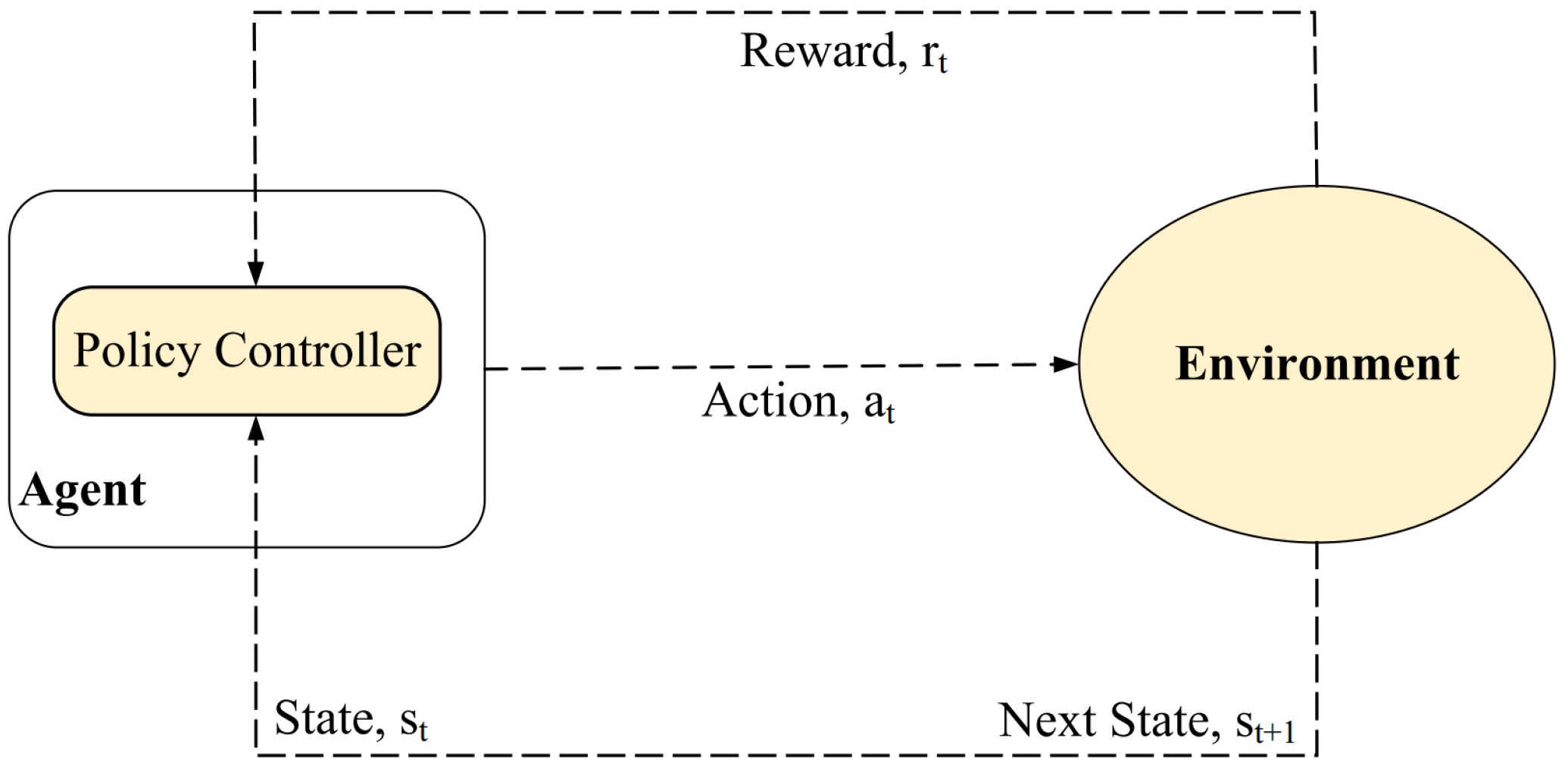
3.1. Reinforcement Learning
3.2. Fuzzy Logic
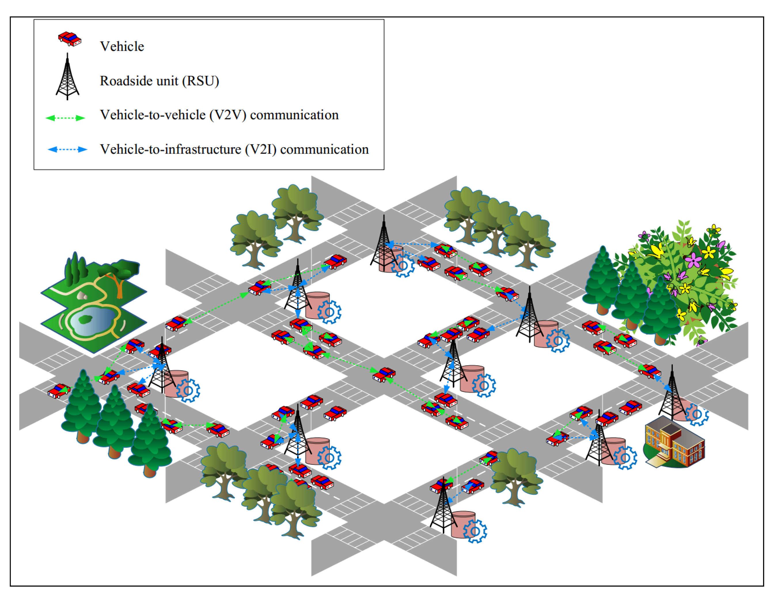
4. Network Model
- Roadside units (RSUs): These components are located at intersections, and their task is to monitor the network and control congestion in each road section. RSUs store a traffic table to record the traffic status of the four road sections connected to the corresponding intersection. This table is periodically updated. Moreover, each RSU holds a Q-table produced by the Q-learning-based routing algorithm to select the best routes between different intersections on the network.
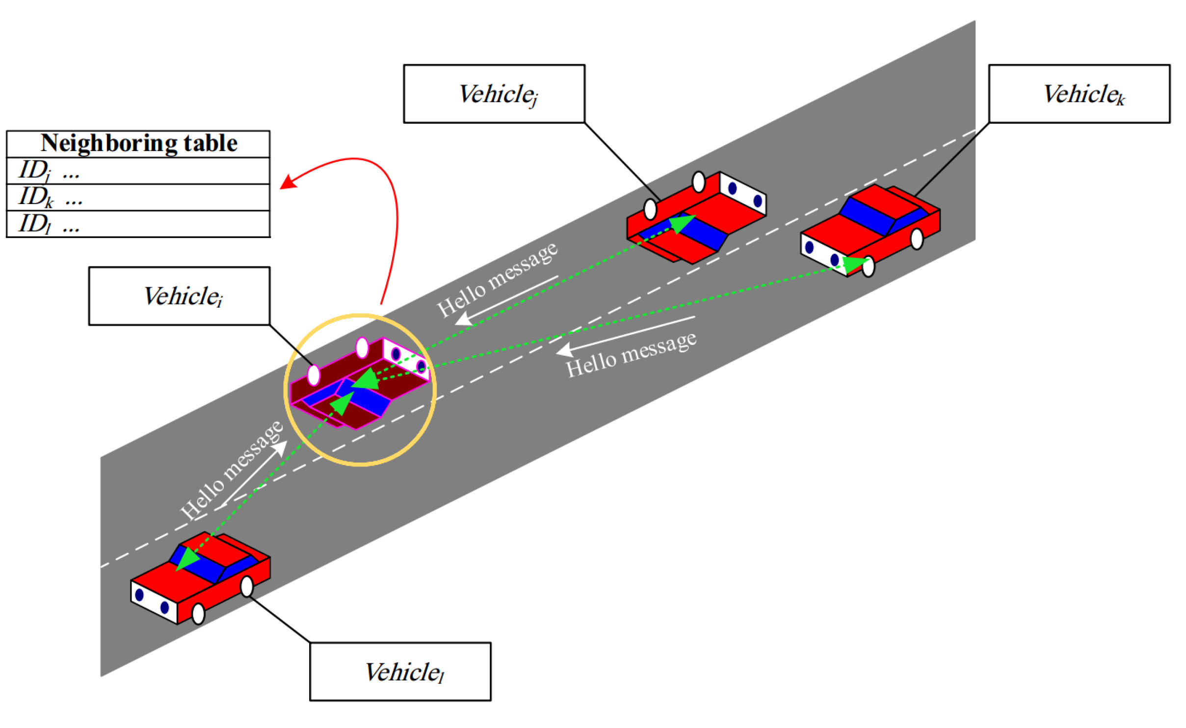
- Vehicles: Each vehicle periodically sends a hello message to its neighboring nodes. These vehicles establish a neighbor table in their memory to store information about neighboring nodes. Additionally, they can achieve their position and speed at any time using a positioning system.
5. Proposed Method
- Identifying traffic conditions;
- Routing algorithm at the intersection level;
- Routing algorithm at the road section level.
5.1. Identifying Traffic Conditions
- Vehicle ID: This field represents the identification of a neighboring vehicle in the road section. After receiving a hello packet from a neighbors, searches its ID in its neighbor table. If this ID is not available in the table, it adds a new entry to this table and records this ID in the ”Vehicle ID” field.
- Road ID: This field is the identification of the road section corresponding to the neighboring vehicle. Upon receiving a new hello message, refreshes the road ID corresponding to the vehicle recorded in its neighbor table.
- Spatial coordinates: It indicates the position of a neighboring vehicle in the road section and is updated after the time period .
- Speed: This field indicates the speed of the neighboring vehicle in the road section. It is fixed at the time period and refreshed after receiving the new hello message.
- Queue status: Using this parameter, can detect the congestion level in the neighboring vehicle. The queue status () is normalized using Equation (3).where, and are the number of packets in the queue and maximum queue length of , respectively.
- Connection quality: It represents the quality of the connection between and . It is measured based on two parameters, namely the connection time and the hello packet reception rate. Section 5.1.1 describes how to calculate this parameter in detail.
- Validity time: It is a time interval when this entry is valid in the neighbor table. After receiving each new hello message from a vehicle, this time interval is refreshed. If the new hello message is not received from the vehicle, the entry related to the vehicle will be removed from the neighbor table after ending the validity time.
5.1.1. Calculating the Connection Quality of Two Vehicles
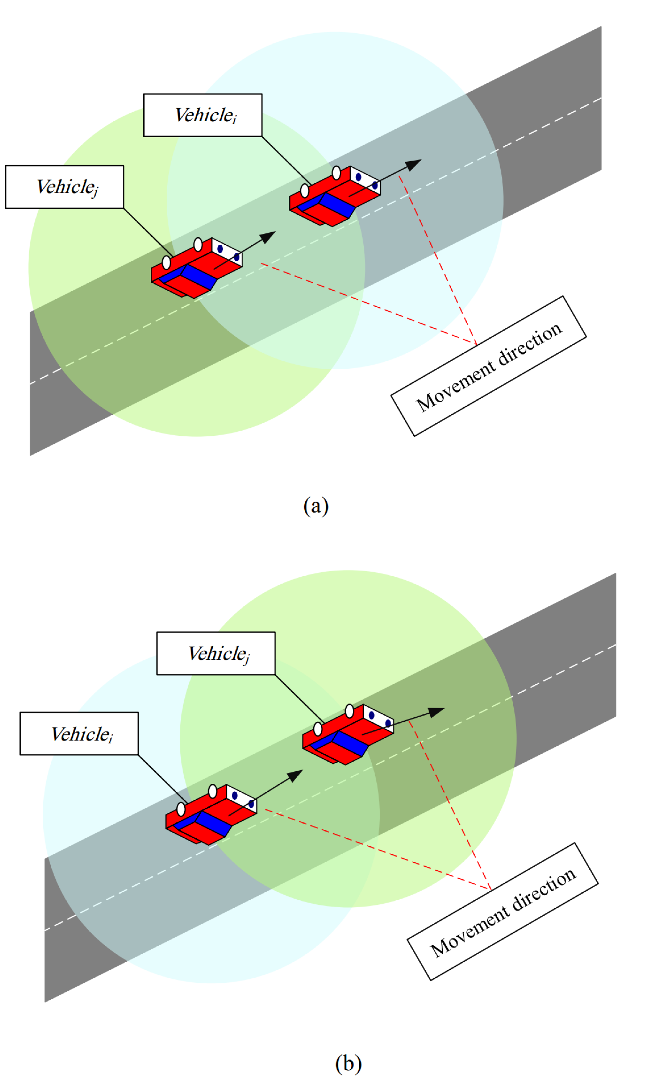
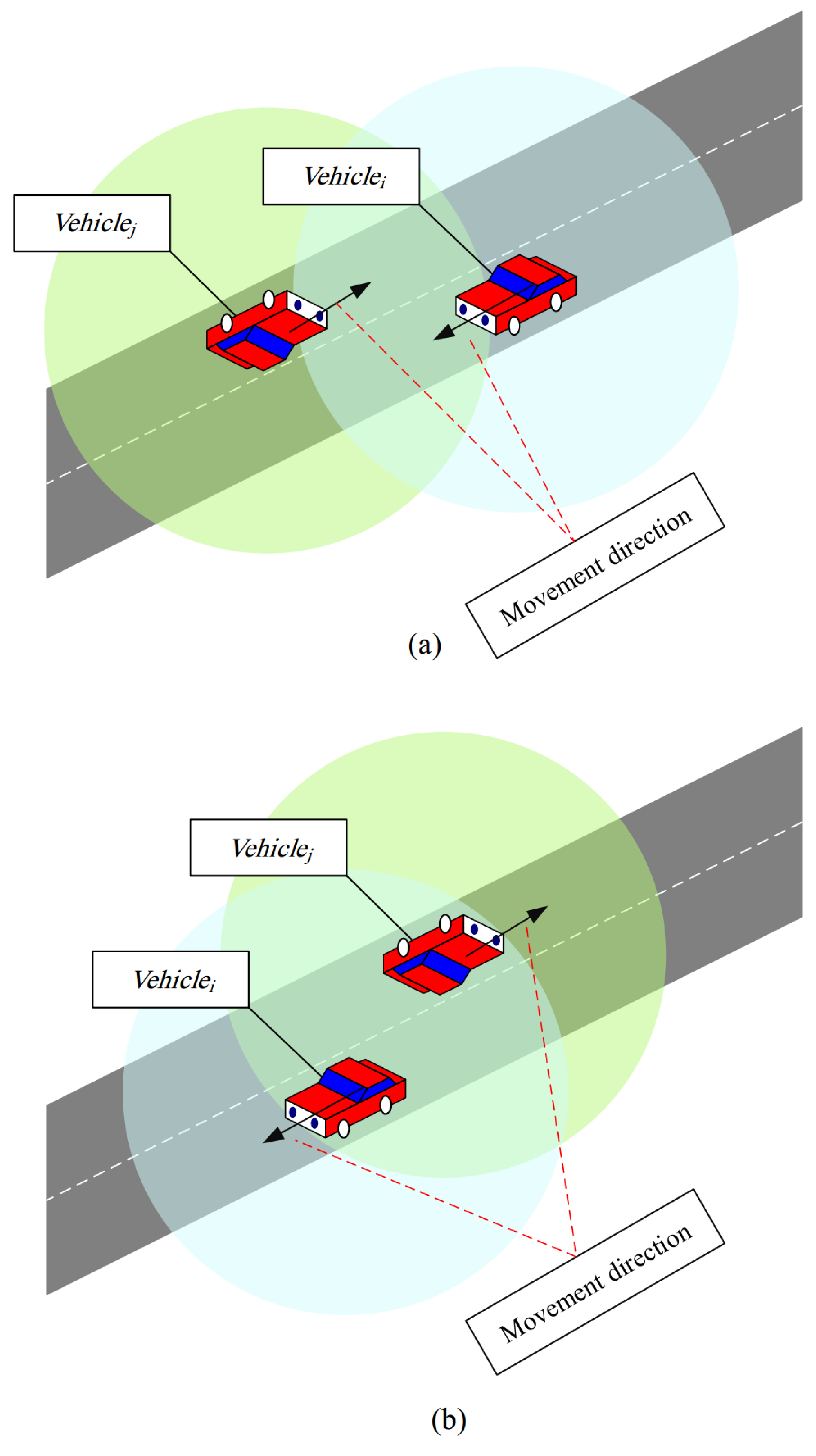
- Connection time (): The connection time of and is evaluated by Equation (5):where, R is the communication radius of vehicles, is the Euclidean distance between the two vehicles and expresses the relative speed of with regard to . Moreover, and represent the spatial coordinates of and , respectively. In addition, and are their speed. is the maximum connection time, which is a fixed value determined based on the simulation time. To accurately estimate the connection time in the dynamic environment of VANET, two configuration coefficients are added to Equation (6). As a result:where, and are the configuration coefficients that are determined as follows:
- Hello packet reception rate (): The quality of the link between and is measured based on the ratio of the hello packages received by to all hello packets transmitted by at the time interval . Each node uses a counter to count the number of hello messages received from its neighbors. Moreover, the hello broadcast time is equal to the specified time frame . As a result, the number of hello messages sent by can be calculated in a certain time . Therefore, each vehicle can calculate the hello reception rate according to Equation (10):where and are equal to the number of received hello messages and the number of sent hello messages, respectively. Then, each vehicle uses Equation (9) to refresh the hello reception rate () using the WMEWMA method.
5.1.2. Forming a Traffic Table
- Neighbor table (): It contains information about neighboring vehicles. The format of this table is presented in Section 5.1. After receiving new hello messages from vehicles in different road sections, RSU searches their IDs in its neighbor table. If these IDs are in the table, RSU updates the recorded information about these vehicles in its neighbor table. Otherwise, RSU adds new entries to this table to record the information about new vehicles.
- Traffic table (): It indicates traffic conditions on the roads connected to the intersection related to RSU. The format of is presented in Table 3. is periodically refreshed every five seconds () because traffic status information at the road level does not change before this time period. includes various fields explained as follows.
- −
- Road ID: Each intersection is connected to the four road sections: the northern road, the southern road, the eastern road, and the western road. The road ID is obtained from the neighbor table.
- −
- Road length: Each RSU (such as ) is aware of its location and the position of its neighboring RSUs (such as ) at adjacent intersections. Therefore, it can calculate the road length using Equation (11):where and are spatial coordinates of and , respectively.
- −
- Average road time (): This field represents the average time required to travel the road section. RSU estimates using Equation (12), which considers two scales, the road length () and the average speed of neighbors in this road section:where is the speed of the neighbors obtained from the neighbor table and is all number of vehicles on the road section. RSU uses the WMEWMA scheme to update using Equation (9) in each road section.
- −
- Vehicle density (): This field represents the number of available vehicles in a road section (i.e., northern, southern, eastern, or western road sections). It is obtained from the neighbor table. To update , RSU uses the WMEWMA method in Equation (9).
- −
- Congestion status (): The value of this field corresponds to the average queue status of vehicles in the road section. It is achieved from the neighbor table:Note that RSU refreshes this parameter in the traffic table using the WMEWMA scheme in Equation (9).
- −
- Average connection quality (): This field represents the average connection quality of vehicles (i.e., ) in each road section. It can be calculated based on Equation (14) and recorded in the traffic table.where is all number of vehicles in the road section R. RSU uses the WMEWMA to update in the traffic table using Equation (9).
- −
- Validity time (): This field represents the time interval that this entry is valid in the traffic table.
| Algorithm 1 Traffic condition detection |
Begin
End |
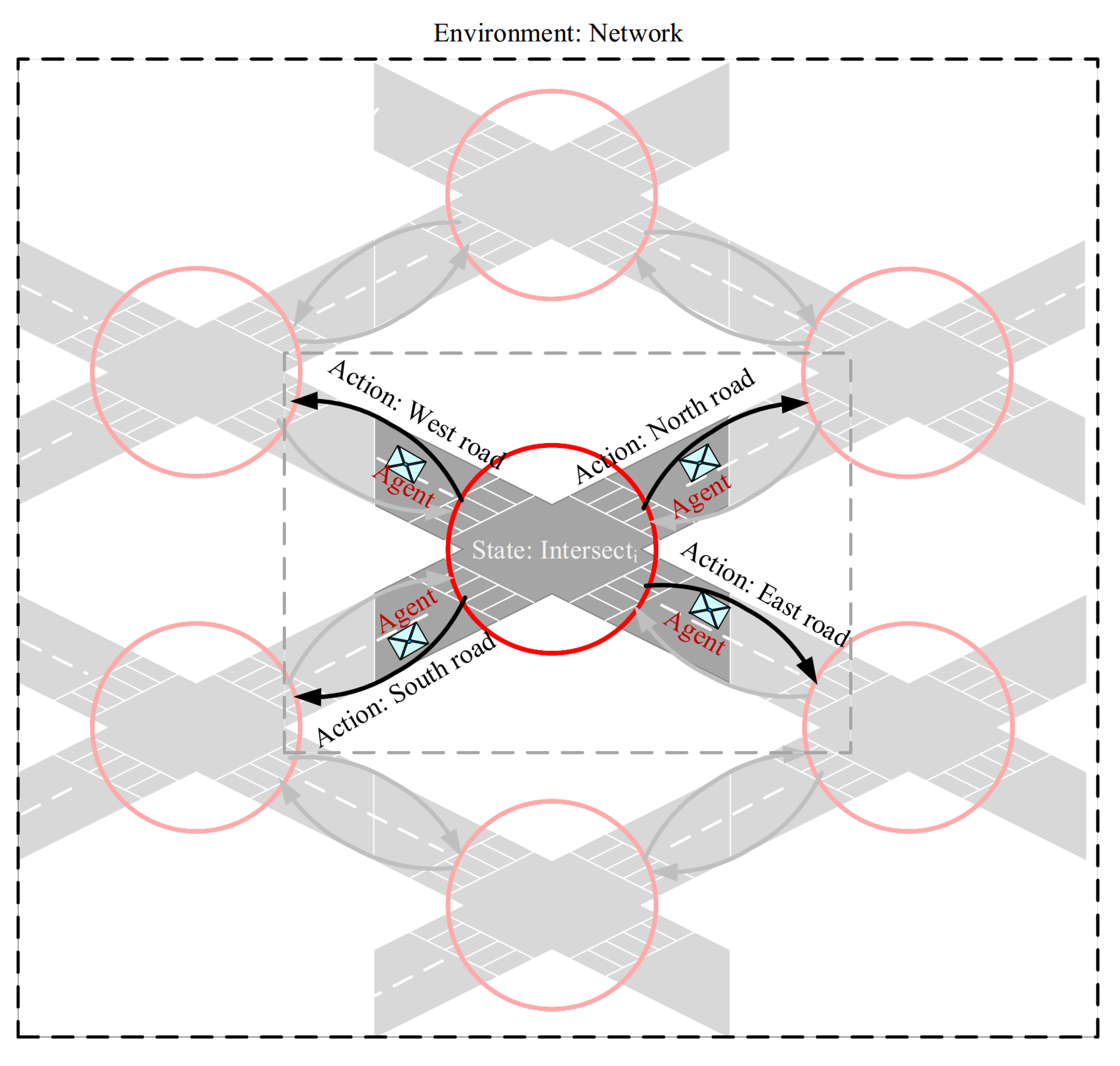
5.2. Routing Algorithm at Intersection Level
| Algorithm 2 Q-learning-based routing algorithm (I2I routing) |
Begin
End |
5.3. Routing Algorithm at the Road Level
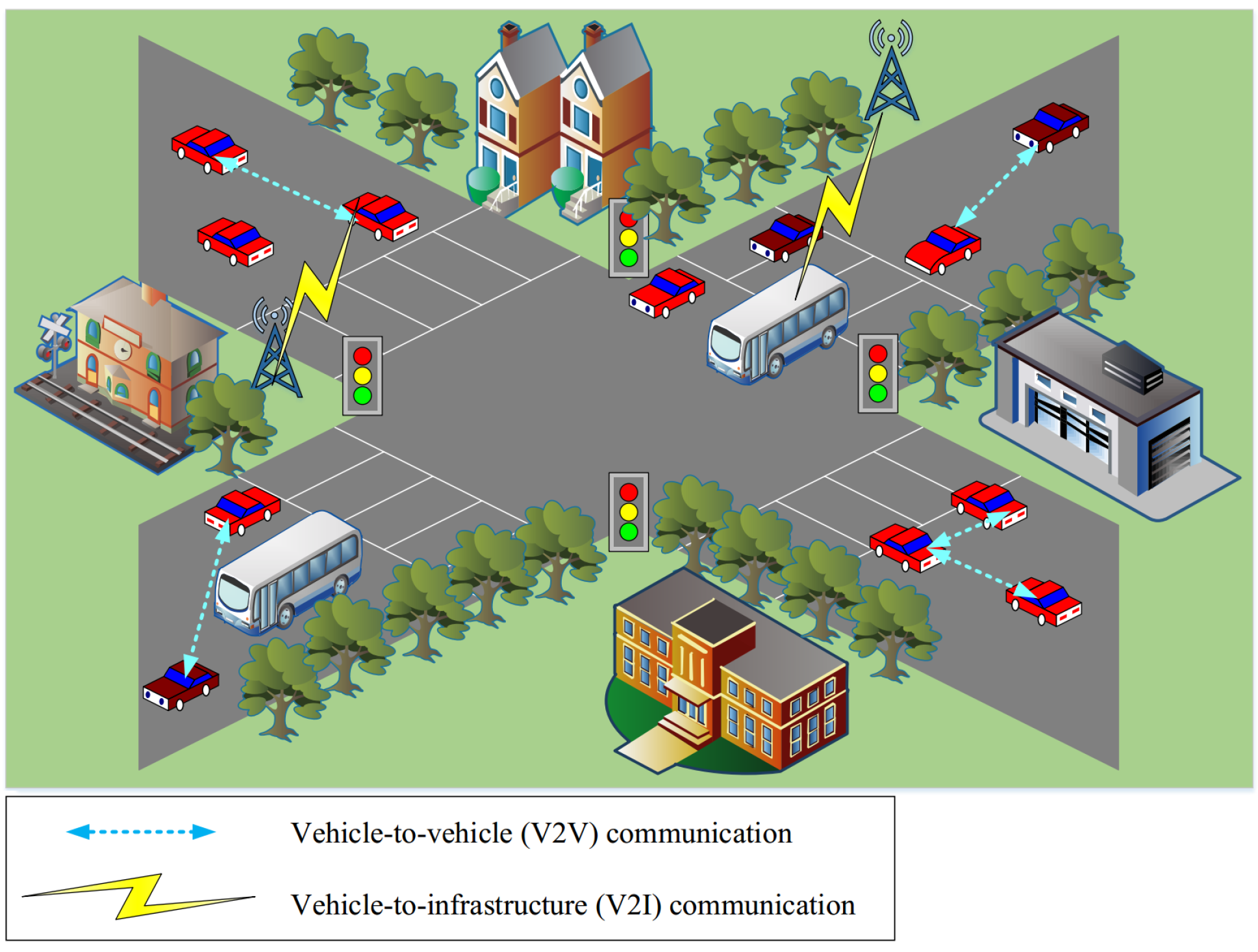
- Vehicle-to-vehicle (V2V) routing algorithm;
- Route recovery algorithm;
- Vehicle-to-infrastructure (V2I) routing algorithm.
5.3.1. Vehicle-to-Vehicle (V2V) Routing Algorithm
- First mode: and move on the same road section. In this case, is determined as a target point ().
- Second mode: and move in different road sections. , which means the source vehicle in this case, considers as .
- Third mode: and move in different road sections. , which is an intermediate vehicle in this case, considers the intersection obtained from Algorithm 2 (i.e., ) as .
5.3.2. Route Recovery Algorithm
Fuzzy Inputs
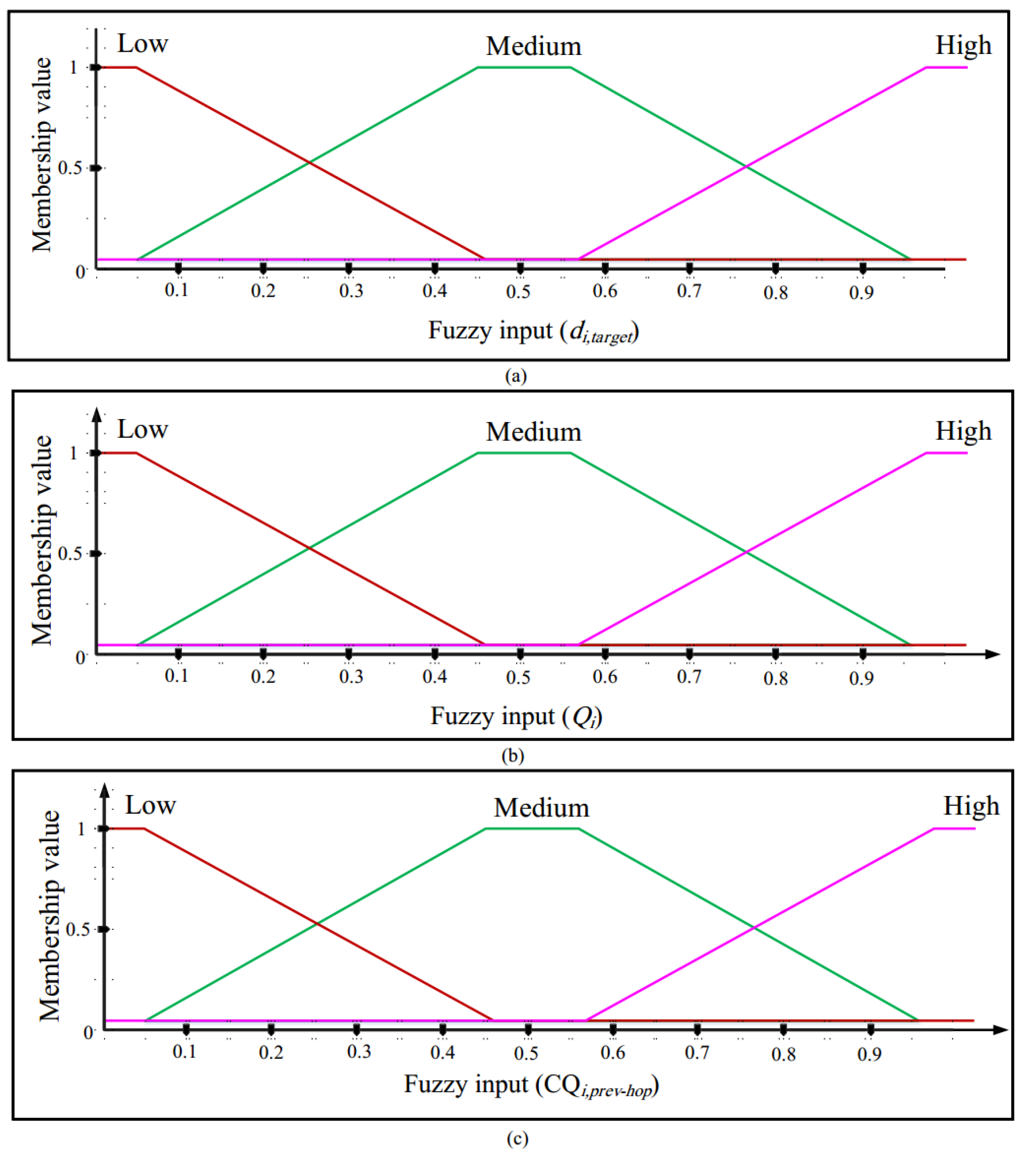
- Distance to (): obtains the distance from a neighboring vehicle (such as ) to with regard to the information stored in the neighbor table based on Equation (17). In this process, the vehicle that is closest to the destination compared to other neighbors gains more chance to be selected as the relay vehicle.where and display the spatial coordinates of and , respectively. Moreover, indicates the length of the road related to . It is calculated using Equation (11). The membership function chart of is presented in Figure 8a. It involves three states: low, medium, and high.
- Queue status (): extracts for each neighboring vehicle (such as ) from the neighbor table. The purpose of this parameter is to lower the chance of vehicles with high traffic being selected as the relay vehicle. See the membership function chart of in Figure 8b. This input considers three states: low, medium, and high.
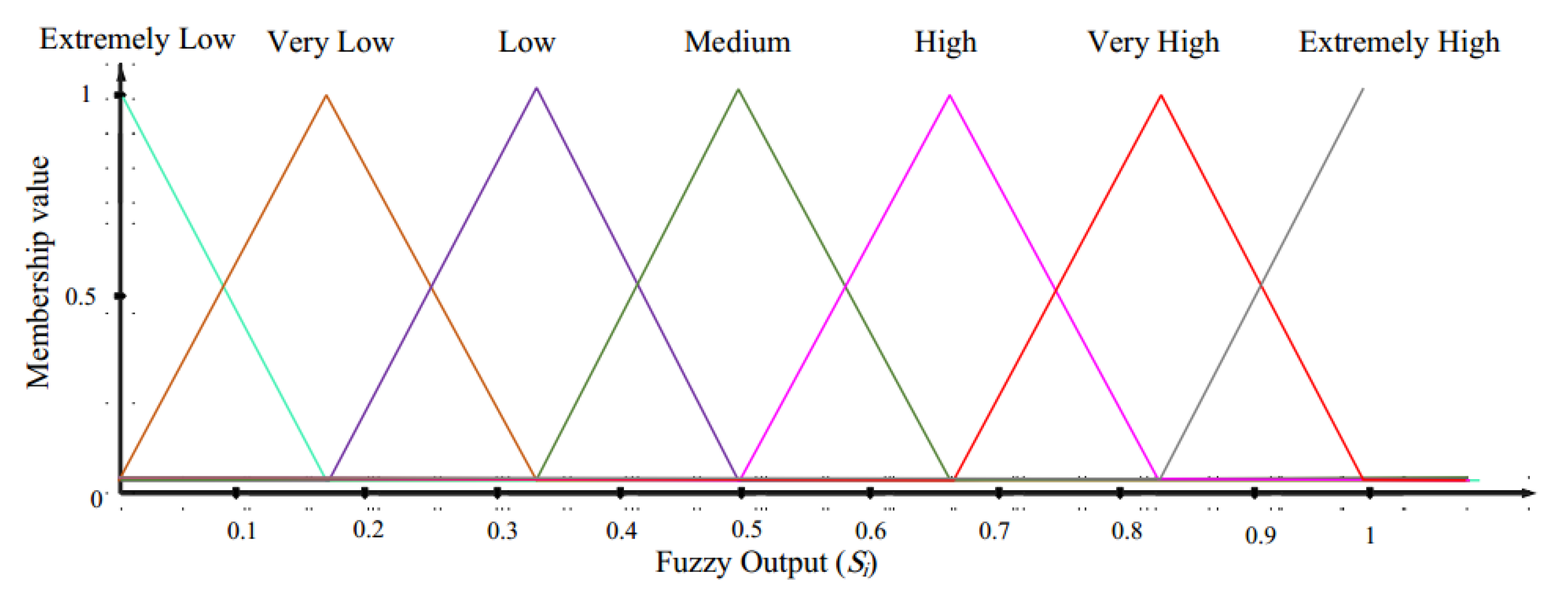
Fuzzy Output
Rule Base
| Algorithm 3 V2V routing process |
Begin
End |
5.3.3. Vehicle-to-Infrastructure (V2I) Routing Algorithm
- First mode: moves in this road section. In this case, is determined as a target point ().
- Second mode: does not move in this road section. In this case, the next intersection is considered as .
| Algorithm 4 V2I routing process |
Begin
End |
6. Simulates and Evaluation of Results
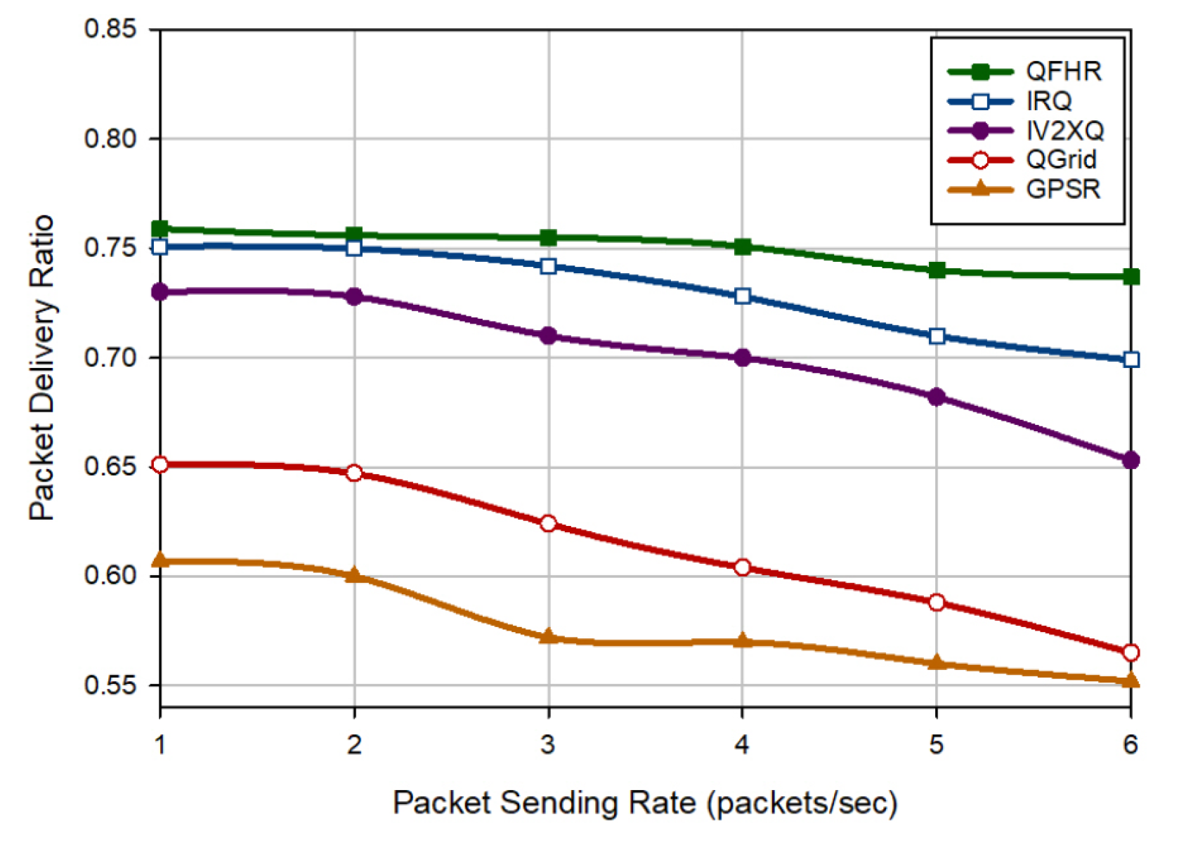
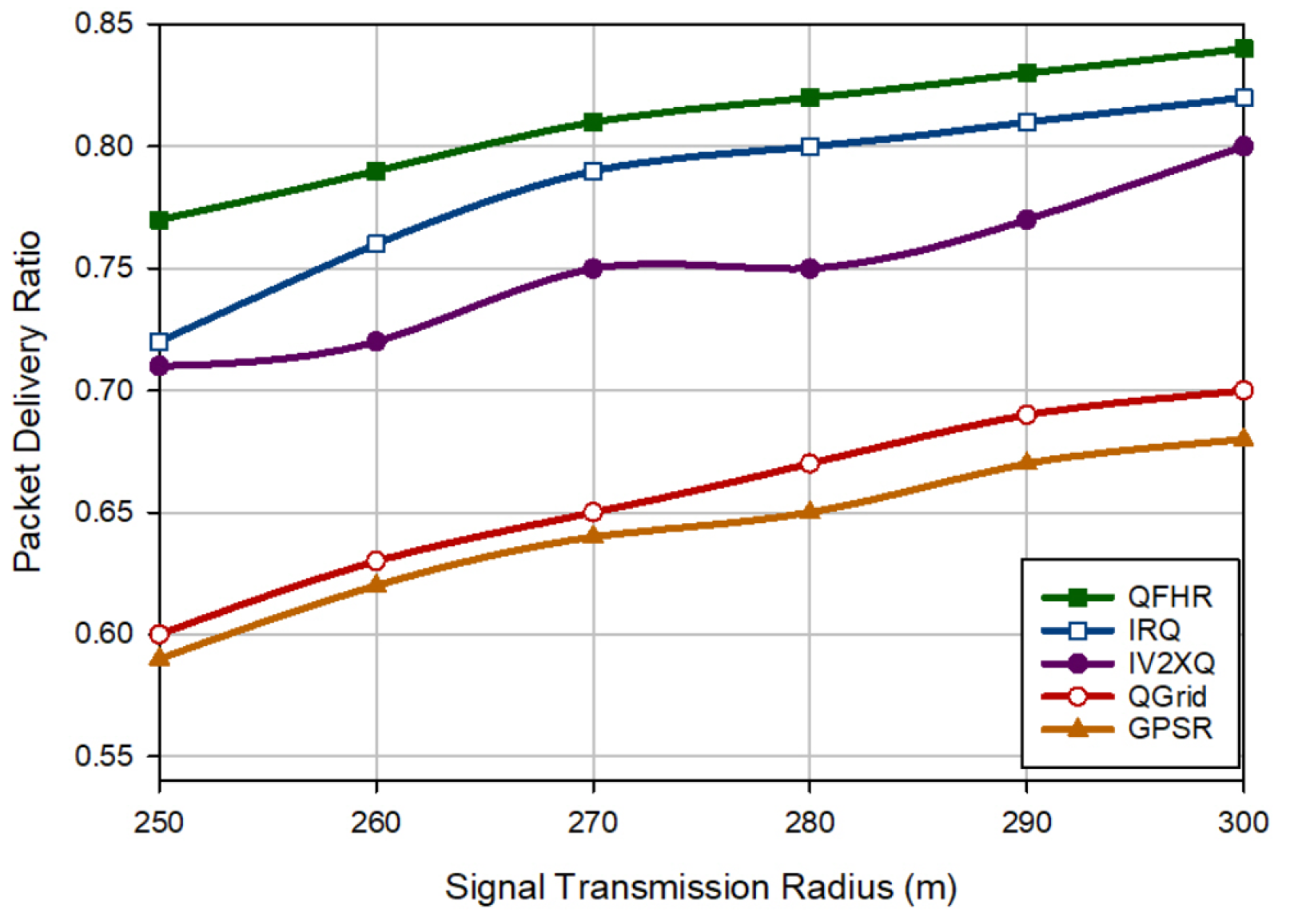
6.1. Packet Delivery Rate (PDR)
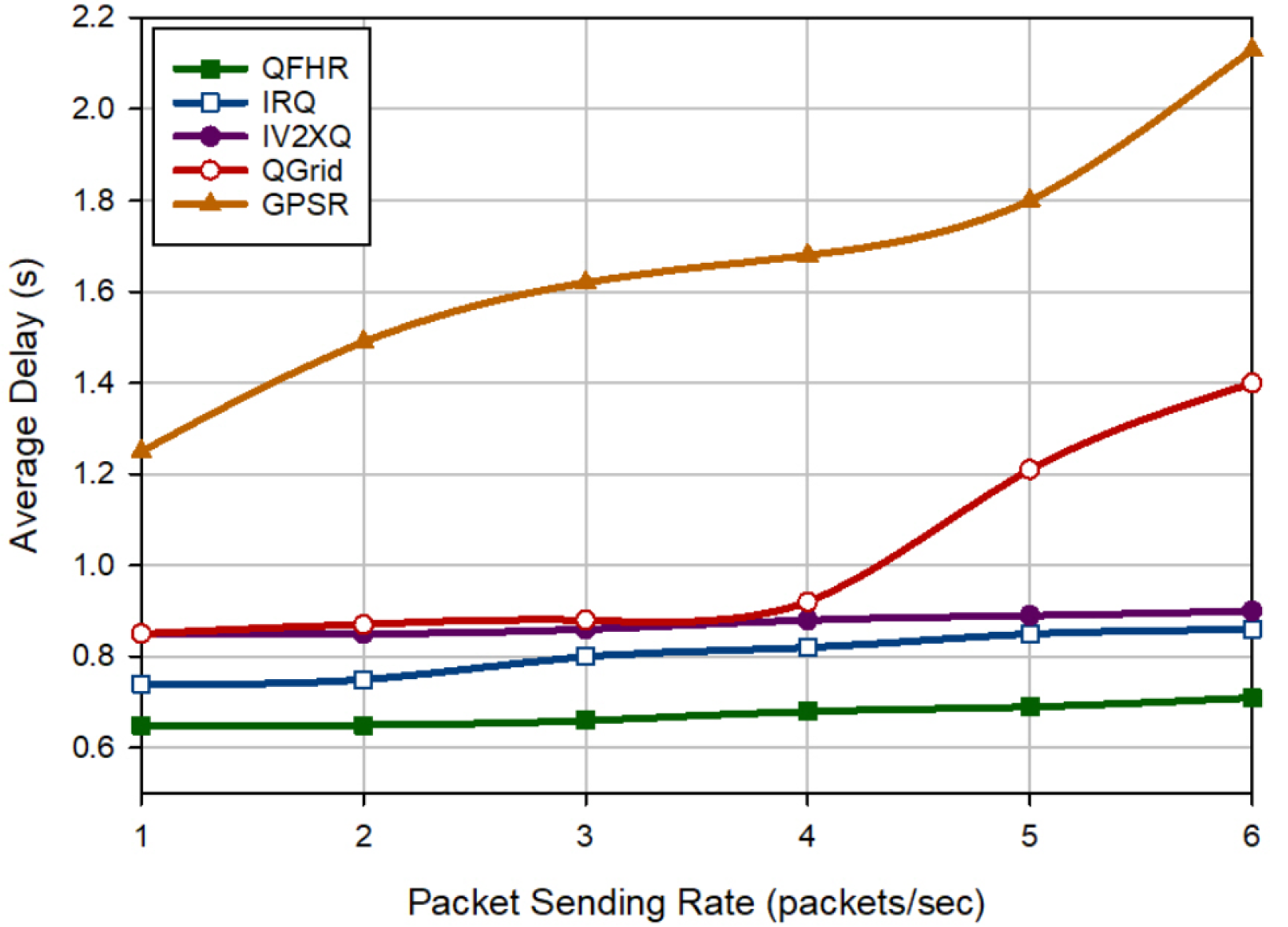
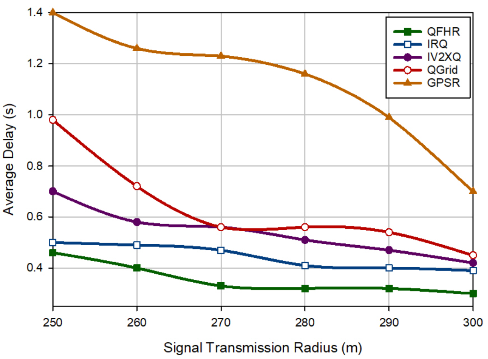
6.2. Delay
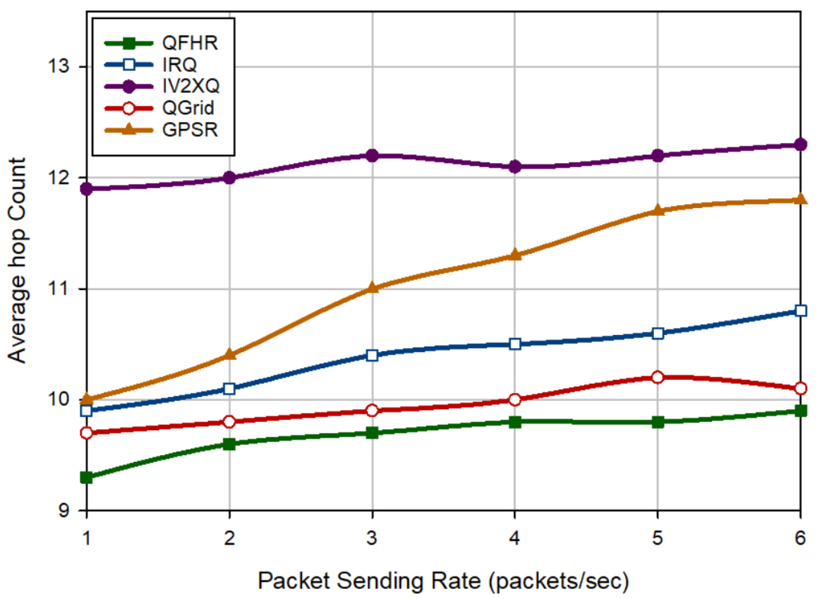
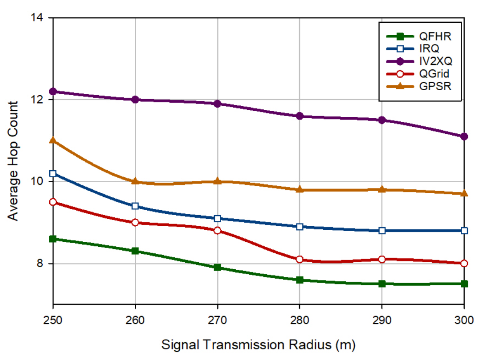
6.3. Hop Count
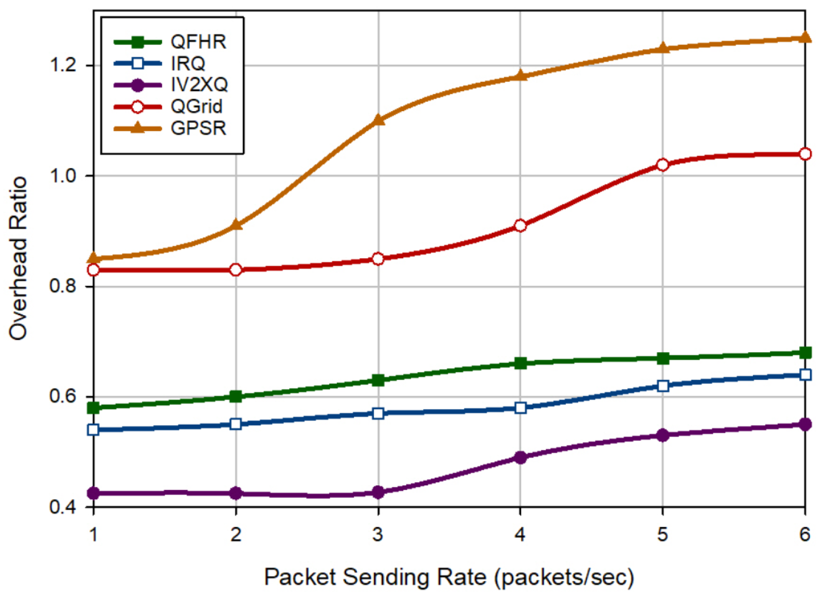
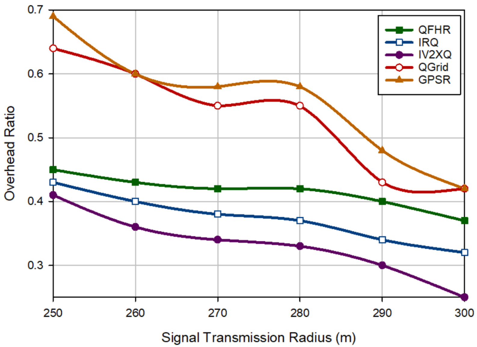
6.4. Routing Overhead
7. Conclusions
Author Contributions
Funding
Data Availability Statement
Conflicts of Interest
References
- Mchergui, A.; Moulahi, T.; Zeadally, S. Survey on Artificial Intelligence (AI) Techniques for Vehicular ad-hoc Networks (VANETs). Veh. Commun. 2021, 100403. [Google Scholar] [CrossRef]
- Xia, Z.; Wu, J.; Wu, L.; Chen, Y.; Yang, J.; Yu, P.S. A comprehensive survey of the key technologies and challenges surrounding vehicular ad hoc networks. ACM Trans. Intell. Syst. Technol. (TIST) 2021, 12, 1–30. [Google Scholar] [CrossRef]
- Abdelgadir, M.; Saeed, R.A.; Babiker, A. Mobility Routing Model for Vehicular ad-hoc Networks (VANETs), Smart City Scenarios. Veh. Commun. 2017, 9, 154–161. [Google Scholar] [CrossRef]
- Li, H.; Liu, Y.; Qin, Z.; Rong, H.; Liu, Q. A large-scale urban vehicular network framework for IoT in smart cities. IEEE Access 2019, 7, 74437–74449. [Google Scholar] [CrossRef]
- Mustakim, H.U. 5G vehicular network for smart vehicles in smart city: A review. J. Comput. Electron. Telecommun. 2020, 1. [Google Scholar] [CrossRef]
- Quy, V.K.; Nam, V.H.; Linh, D.M.; Ban, N.T.; Han, N.D. Communication Solutions for Vehicle ad-hoc Network in Smart Cities Environment: A Comprehensive Survey. Wirel. Pers. Commun. 2021, 122, 2791–2815. [Google Scholar] [CrossRef]
- Li, F.; Wang, Y. Routing in vehicular ad hoc networks: A survey. IEEE Veh. Technol. Mag. 2007, 2, 12–22. [Google Scholar] [CrossRef]
- Domingos, F.; Villas, L.; Boukerche, A. Data Communication in VANETs: Survey, Applications and Challenges. Ad Hoc Netw. 2016, 44, 90–103. [Google Scholar]
- Lee, S.W.; Ali, S.; Yousefpoor, M.S.; Yousefpoor, E.; Lalbakhsh, P.; Javaheri, D.; Rahmani, A.M.; Hosseinzadeh, M. An energy-aware and predictive fuzzy logic-based routing scheme in flying ad hoc networks (fanets). IEEE Access 2021, 9, 129977–130005. [Google Scholar] [CrossRef]
- Rahmani, A.M.; Ali, S.; Yousefpoor, M.S.; Yousefpoor, E.; Naqvi, R.A.; Siddique, K.; Hosseinzadeh, M. An area coverage scheme based on fuzzy logic and shuffled frog-leaping algorithm (sfla) in heterogeneous wireless sensor networks. Mathematics 2021, 9, 2251. [Google Scholar] [CrossRef]
- Dua, A.; Kumar, N.; Bawa, S. A Systematic Review on Routing Protocols for Vehicular ad hoc Networks. Veh. Commun. 2014, 1, 33–52. [Google Scholar] [CrossRef]
- Boussoufa-Lahlah, S.; Semchedine, F.; Bouallouche-Medjkoune, L. Geographic routing protocols for Vehicular Ad hoc NETworks (VANETs): A survey. Veh. Commun. 2018, 11, 20–31. [Google Scholar] [CrossRef]
- Aggarwal, A.; Gaba, S.; Nagpal, S.; Vig, B. Bio-Inspired Routing in VANET. Cloud IoT-Based Veh. Ad Hoc Netw. 2021, 199–220. [Google Scholar] [CrossRef]
- Ksouri, C.; Jemili, I.; Mosbah, M.; Belghith, A. Towards general Internet of Vehicles networking: Routing protocols survey. Concurr. Comput. Pract. Exp. 2022, 34, e5994. [Google Scholar] [CrossRef]
- Teixeira, L.H.; Huszák, Á. Reinforcement Learning Environment for Advanced Vehicular Ad Hoc Networks Communication Systems. Sensors 2022, 22, 4732. [Google Scholar] [CrossRef] [PubMed]
- Pateria, S.; Subagdja, B.; Tan, A.H.; Quek, C. Hierarchical reinforcement learning: A comprehensive survey. ACM Comput. Surv. (CSUR) 2021, 54, 1–35. [Google Scholar] [CrossRef]
- Genders, W.; Razavi, S. Asynchronous n-step Q-learning adaptive traffic signal control. J. Intell. Transp. Syst. 2019, 23, 319–331. [Google Scholar] [CrossRef]
- Chen, X.; Wu, S.; Shi, C.; Huang, Y.; Yang, Y.; Ke, R.; Zhao, J. Sensing data supported traffic flow prediction via denoising schemes and ANN: A comparison. IEEE Sens. J. 2020, 20, 14317–14328. [Google Scholar] [CrossRef]
- Gronauer, S.; Diepold, K. Multi-agent deep reinforcement learning: A survey. Artif. Intell. Rev. 2022, 55, 895–943. [Google Scholar] [CrossRef]
- Chen, W.; Qiu, X.; Cai, T.; Dai, H.N.; Zheng, Z.; Zhang, Y. Deep reinforcement learning for Internet of Things: A comprehensive survey. IEEE Commun. Surv. Tutor. 2021, 23, 1659–1692. [Google Scholar] [CrossRef]
- Sun, Y.; Lin, Y.; Tang, Y. A reinforcement learning-based routing protocol in VANETs. In International Conference in Communications, Signal Processing, and Systems; Springer: Singapore, 2017; pp. 2493–2500. [Google Scholar] [CrossRef]
- Roh, B.S.; Han, M.H.; Ham, J.H.; Kim, K.I. Q-LBR: Q-learning based load balancing routing for UAV-assisted VANET. Sensors 2020, 20, 5685. [Google Scholar] [CrossRef] [PubMed]
- Bi, X.; Gao, D.; Yang, M. A reinforcement learning-based routing protocol for clustered EV-VANET. In Proceedings of the 2020 IEEE 5th Information Technology and Mechatronics Engineering Conference (ITOEC), Chongqing, China, 12–14 June 2020; pp. 1769–1773. [Google Scholar] [CrossRef]
- Yang, X.; Zhang, W.; Lu, H.; Zhao, L. V2V routing in VANET based on heuristic Q-learning. Int. J. Comput. Commun. Control 2020, 15. [Google Scholar] [CrossRef]
- Wu, C.; Yoshinaga, T.; Bayar, D.; Ji, Y. Learning for adaptive anycast in vehicular delay tolerant networks. J. Ambient Intell. Humaniz. Comput. 2019, 10, 1379–1388. [Google Scholar] [CrossRef]
- Karp, B.; Kung, H.T. GPSR: Greedy perimeter stateless routing for wireless networks. In Proceedings of the 6th Annual International Conference on Mobile Computing and Networking, Boston, MA, USA, 6–11 August 2000; pp. 243–254. [Google Scholar]
- Li, F.; Song, X.; Chen, H.; Li, X.; Wang, Y. Hierarchical routing for vehicular ad hoc networks via reinforcement learning. IEEE Trans. Veh. Technol. 2018, 68, 1852–1865. [Google Scholar] [CrossRef]
- Luo, L.; Sheng, L.; Yu, H.; Sun, G. Intersection-based V2X routing via reinforcement learning in vehicular Ad Hoc networks. IEEE Trans. Intell. Transp. Syst. 2021, 23, 5446–5459. [Google Scholar] [CrossRef]
- Khan, M.U.; Hosseinzadeh, M.; Mosavi, A. An Intersection-Based Routing Scheme Using Q-Learning in Vehicular Ad Hoc Networks for Traffic Management in the Intelligent Transportation System. Mathematics 2022, 10, 3731. [Google Scholar] [CrossRef]
- Rezwan, S.; Choi, W. A survey on applications of reinforcement learning in flying ad-hoc networks. Electronics 2021, 10, 449. [Google Scholar] [CrossRef]
- Padakandla, S. A survey of reinforcement learning algorithms for dynamically varying environments. ACM Comput. Surv. (CSUR) 2021, 54, 1–25. [Google Scholar] [CrossRef]
- Al-Rawi, H.A.; Ng, M.A.; Yau, K.L.A. Application of reinforcement learning to routing in distributed wireless networks: A review. Artif. Intell. Review. 2015, 43, 381–416. [Google Scholar] [CrossRef]
- Rahmani, A.M.; Yousefpoor, E.; Yousefpoor, M.S.; Mehmood, Z.; Haider, A.; Hosseinzadeh, M.; Ali Naqvi, R. Machine learning (ML) in medicine: Review, applications, and challenges. Mathematics 2021, 9, 2970. [Google Scholar] [CrossRef]
- Dumitrescu, C.; Ciotirnae, P.; Vizitiu, C. Fuzzy logic for intelligent control system using soft computing applications. Sensors 2021, 21, 2617. [Google Scholar] [CrossRef] [PubMed]
- Nadaban, S. From classical logic to fuzzy logic and quantum logic: A general view. Int. J. Comput. Commun. Control 2021, 16. [Google Scholar] [CrossRef]
- van Krieken, E.; Acar, E.; van Harmelen, F. Analyzing differentiable fuzzy logic operators. Artif. Intell. 2022, 302, 103602. [Google Scholar] [CrossRef]
- Perry, M.B. The exponentially weighted moving average. Wiley Encycl. Oper. Res. Manag. Sci. 2010. [Google Scholar] [CrossRef]
- Nabi, M.; Geilen, M.M.; Basten, T.A. An empirical study of link quality estimation techniques for disconnection detection in WBANs. In Proceedings of the 16th ACM International Conference on Modeling, Analysis & Simulation of Wireless and Mobile Systems, Barcelona, Spain, 3–8 November 2013; pp. 219–228. [Google Scholar]
- Altman, E.; Jimenez, T. NS Simulator for beginners. Synth. Lect. Commun. Netw. 2012, 5, 1–184. [Google Scholar]


| Method | Strengths | Weaknesses |
|---|---|---|
| PbQR [21] | Stability of communication links, improving packet transmission rate, reducing delay in the routing process, high scalability | Applying a greedy approach to obtain Q-value from Q-table, high dependence on RSU, not considering traffic lights as warning signs |
| Q-LBR [22] | Low routing overhead, high packet transmission rate, stability of communication links, suitable for urban areas during natural disasters, high scalability | Not considering a mechanism for adding drones to the network, not providing techniques to calculate the optimal height of drones, not specifying the number of drones |
| RLRC [23] | Considering the optimal energy consumption in electric vehicles, using SARSA for optimizing the routing process, scalability | High bandwidth consumption, high delay, low throughput, not paying attention to motion direction |
| HQVR [24] | Determining the learning rate based on the link quality, increasing packet delivery rate, reducing the effect of the node mobility on the convergence speed of Q-learning algorithm, low dependence on infrastructure (RSUs) | High dependence of Q-learning algorithm to beacon messages, slow convergence speed of the learning algorithm, applying an exploration technique based on a specific probability |
| QVDRP [25] | High delay-tolerant, increasing packet delivery rate, reducing the number of duplicated control messages, considering relative velocity of vehicles | Slow convergence speed of the learning algorithm |
| GPSR [26] | Reducing routing overhead, reducing delay in the network | Not considering factors, like velocity, movement direction, and link lifetime in the routing process |
| QGrid [27] | Reducing the number of states in Q-learning algorithm, appropriate convergence speed, reducing communication overhead, determining the discount factor based on vehicle density | Designing an off-line routing, not designing a congestion control mechanism in the network, fixing Q-table during the simulation process, not considering the effect of intersections and buildings on the transmission quality in each grid, not considering parameters such as speed, movement direction, and link lifetime in the routing process, introducing a centralized reinforcement learning-based routing algorithm |
| IV2XQ [28] | Determining the discount factor with regard to the density and distance of vehicles on the road section, reducing communication overhead, designing a congestion control mechanism, appropriate convergence speed, reducing the number of states in the Q-learning algorithm | Not considering factors, like speed, movement direction, and link lifetime in the routing process, not relying on new traffic information in the network, introducing a centralized reinforcement learning-based routing algorithm |
| IRQ [29] | Adjusting the discount factor with regard to the vehicle density and distance, high PDR, reducing latency in the routing process, presenting a evaluation mechanism for controlling the congested paths, suitable convergence speed, reducing the number of states in the Q-learning algorithm, considering new traffic information in the network | High routing overhead, introducing a centralized reinforcement learning-based routing algorithm |
| Vehicle ID | Road ID | Spatial Coordinates | Speed | Queue Status | Connection Quality | Validity Time |
|---|---|---|---|---|---|---|
| Road ID | Road Length | Average Road Time | Vehicle Density | Congestion Status | Average Connection Quality | Validity Time |
|---|---|---|---|---|---|---|
| Northern road length | Average northern road time | The number of vehicles in the northern road | Average congestion status in the northern road | Average connection quality in the northern road | ||
| Southern road length | Average southern road time | The number of vehicles in the southern road | Average congestion status in the southern road | Average connection quality in the southern road | ||
| Eastern road length | Average eastern road time | The number of vehicles in the eastern road | Average congestion status in the eastern road | Average connection quality in the eastern road | ||
| Western road length | Average western road time | The number of vehicles in the western road | Average congestion status in the western road | Average connection quality in the western road |
| Fuzzy System Inputs | Fuzzy System Output | |||
|---|---|---|---|---|
| Fuzzy Rules | ||||
| 1 | Low | Low | Low | High |
| 2 | Low | Low | Medium | Very high |
| 3 | Low | Low | High | Extermely high |
| 4 | Low | Medium | Low | Medium |
| 5 | Low | Medium | Medium | High |
| 6 | Low | Medium | High | Very high |
| 7 | Low | High | Low | Low |
| 8 | Low | High | Medium | Medium |
| 9 | Low | High | High | High |
| 10 | Medium | Low | Low | Medium |
| 11 | Medium | Low | Medium | High |
| 12 | Medium | Low | High | Very high |
| 13 | Medium | Medium | Low | Low |
| 14 | Medium | Medium | Medium | Medium |
| 15 | Medium | Medium | High | High |
| 16 | Medium | High | Low | Very low |
| 17 | Medium | High | Medium | Low |
| 18 | Medium | High | High | Medium |
| 19 | High | Low | Low | Low |
| 20 | High | Low | Medium | Medium |
| 21 | High | Low | High | High |
| 22 | High | Medium | Low | Very low |
| 23 | High | Medium | Medium | Low |
| 24 | High | Medium | High | Medium |
| 25 | High | High | Low | Extermely low |
| 26 | High | High | Medium | Very low |
| 27 | High | High | High | Low |
| Parameters | Value |
|---|---|
| Network simulator | NS2 |
| Network size | km2 |
| Simulation time | 1000 s |
| Vehicles | 450 |
| Road sections | 38 |
| Intersections | 24 |
| Vehicle density | 0.005–0.02 (Vehicle/m) |
| Vehicle velocity | 14 m/s |
| Communication range of vehicles | 250–300 m |
| Communication range of RSUs | 300 m |
| Packet size | 512 byte |
| Packet sending rate | 1–6 (Packet/s) |
| Hello broadcast period | 1 s |
| Learning rate () | 0.1 |
| 0.2 |
Publisher’s Note: MDPI stays neutral with regard to jurisdictional claims in published maps and institutional affiliations. |
© 2022 by the authors. Licensee MDPI, Basel, Switzerland. This article is an open access article distributed under the terms and conditions of the Creative Commons Attribution (CC BY) license (https://creativecommons.org/licenses/by/4.0/).
Share and Cite
Rahmani, A.M.; Naqvi, R.A.; Yousefpoor, E.; Yousefpoor, M.S.; Ahmed, O.H.; Hosseinzadeh, M.; Siddique, K. A Q-Learning and Fuzzy Logic-Based Hierarchical Routing Scheme in the Intelligent Transportation System for Smart Cities. Mathematics 2022, 10, 4192. https://doi.org/10.3390/math10224192
Rahmani AM, Naqvi RA, Yousefpoor E, Yousefpoor MS, Ahmed OH, Hosseinzadeh M, Siddique K. A Q-Learning and Fuzzy Logic-Based Hierarchical Routing Scheme in the Intelligent Transportation System for Smart Cities. Mathematics. 2022; 10(22):4192. https://doi.org/10.3390/math10224192
Chicago/Turabian StyleRahmani, Amir Masoud, Rizwan Ali Naqvi, Efat Yousefpoor, Mohammad Sadegh Yousefpoor, Omed Hassan Ahmed, Mehdi Hosseinzadeh, and Kamran Siddique. 2022. "A Q-Learning and Fuzzy Logic-Based Hierarchical Routing Scheme in the Intelligent Transportation System for Smart Cities" Mathematics 10, no. 22: 4192. https://doi.org/10.3390/math10224192