
Distributionally Robust Optimization Model for a Minimum Cost Consensus with Asymmetric Adjustment Costs Based on the Wasserstein Metric

1
Alibaba, Hangzhou 311121, China
2
Business School, University of Shanghai for Science and Technology, Shanghai 200093, China
3
School of Management Science and Technology, Nanjing University of Information Science and Technology, Nanjing 210000, China
*
Author to whom correspondence should be addressed.
Mathematics 2022, 10(22), 4312; https://doi.org/10.3390/math10224312
Submission received: 28 August 2022
/
Revised: 4 November 2022
/
Accepted: 9 November 2022
/
Published: 17 November 2022
(This article belongs to the Special Issue Collaborative Decision-Making Analysis and Applications)
Abstract
:When solving the problem of the minimum cost consensus with asymmetric adjustment costs, decision makers need to face various uncertain situations (such as individual opinions and unit adjustment costs for opinion modifications in the up and down directions). However, in the existing methods for dealing with this problem, robust optimization will lead to overly conservative results, and stochastic programming needs to know the exact probability distribution. In order to overcome these shortcomings, it is essential to develop a novelty consensus model. Thus, we propose three new minimum-cost consensus models with a distributionally robust method. Uncertain parameters (individual opinions, unit adjustment costs for opinion modifications in the up and down directions, the degree of tolerance, and the range of thresholds) were investigated by modeling the three new models, respectively. In the distributionally robust method, the construction of an ambiguous set is very important. Based on the historical data information, we chose the Wasserstein ambiguous set with the Wasserstein distance in this study. Then, three new models were transformed into a second-order cone programming problem to simplify the calculations. Further, a case from the EU Trade and Animal Welfare (TAW) program policy consultation was used to verify the practicability of the proposed models. Through comparison and sensitivity analysis, the numerical results showed that the three new models fit the complex decision environment better.
1. Introduction
Group decision-making (GDM) is a current hot research direction in the field of decision science [1,2,3,4,5,6], and it can be applied in practical scenarios, such as the environmental management project in the Yangtze River Delta region or how institutions choose stocks during the COVID-19 crisis [7]. GDM plays a crucial role in both preliminary planning and project implementation.
In GDM research, consensus-reaching is a basic research content and is the most complex aspect in this field [8]. Consensus-reaching can be seen as the result of the coordinated consistency of group opinions or the convergence of opinions. GDM is essentially a multiround coordination problem involving multiple interactions [9]. Decision makers (DMs) express their opinions based on their decision preferences. However, in most cases, it is difficult for the DMs to obtain a satisfactory consensus opinion because different DMs are in different groups and have the characteristics of different interest groups. Thus, it requires DMs to continuously revise their initial decision opinions to reach a consensus [10]. When DMs have different opinions on the same problem, they want to maintain their original opinion and a final consensus cannot be reached. In this case, GDM needs a moderator with excellent communication skills and leadership who will convince them to change their opinions, and the moderator will spend some cost, such as providing time or money compensation during coordination. From a practical point of view, the moderator always wants to solve the problem efficiently with the minimum cost and within the shortest time. Therefore, it is necessary to study how to reach a consensus with the minimum cost [11].
Based on this practical background, in 2007, Ben-Arieh et al. [12] first pointed out the importance of the costs and deviations of DMs’ opinions and proposed the concept of the minimum cost consensus model (MCCM) to characterize the costs and DMs’ opinions. Finally, a linear time algorithm for all cost consensus problems was proposed. Unfortunately, the research results did not specifically propose a research model of consensus cost. According to the previous research, Ben-Arieh et al. [13] further proposed a consensus-reaching method based on quadratic cost and the model became the basis for future research. Zhang et al. [11] studied the minimum cost consensus model and combined the aggregation operator with the model to consider the consensus opinion. However, in this model, the conditions for reaching a consensus were very strict. In order to make the model more consistent with real life, Zhang et al. [14] put forward the concept of soft cost consensus, and a new model under a certain consensus level was structured, which can be called an MCCM with a weighted average operator, reconstructed a maximum objective model through its dual model, and applied it to the field of online lending to verify the validity of the model. Up to now, many scholars have adopted various methods to improve the MCCM [15,16,17,18].
Previous studies assumed that the unit adjustment cost in different directions is symmetrical, but in many real scenarios, the unit adjustment costs are not symmetrical. For example, in the establishment of environmental standards, local governments will have different expectations of standards due to differences in economic development status, technical conditions, geographical factors, and residents’ awareness of environmental protection; therefore, the costs of adjusting their opinions in different directions may not be symmetrical. Therefore, the research on asymmetric adjustment costs has practical significance. Based on this research idea, Cheng et al. [19] considered that the study of asymmetric cost has a certain significance and further thought that the compromise of each DM has a limit and the opinion adjustment has a threshold value; they then constructed three cost consensus models.
One purpose of this study was to investigate the realistic impact of asymmetric costs in detail. However, whether it is a model with asymmetric costs or a model with symmetric costs, an implicit assumption of models is that the unit adjustment costs and DMs’ opinions can be known exactly. As is known to all, uncertainty in the real world is normal and the data of real life is uncertain due to many reasons, such as prediction errors, measurement errors, or implementation errors. If we do not consider the uncertain influences in the models, our proposed models will fail owing to the disturbance of data. Therefore, another purpose of this study was to investigate the impact of uncertainty on the proposed models.
Nowadays, more and more scholars are studying uncertainty in MCCM [20,21,22,23,24]. Han et al. [25] pioneered the combination of a robust optimization method with the consensus cost problem, which considers that perturbations in the input data during GDM may degrade the quality of the optimal solution, and therefore, a robust optimization method is used to overcome the uncertainty in the unit adjustment cost. The numerical experiments in this study demonstrated that the traditional MCCM has overly optimistic results and the improved consensus model is more robust. Based on the previous study, Qu et al. [26] further investigated the consensus model based on an asymmetric adjustment cost and set uncertain parameters in the unit adjustment cost. Finally, cost consensus models for three MCCMs with directional restrictions were developed, the results of four uncertainty sets were compared with previous models, and the final data showed that the robust model with an interval-polyhedral set had the lowest consensus cost and guaranteed the robustness of the results. Jin et al. [27] considered multi-attribute decision problems: in order to achieve their own interests, different interest groups or individuals will intentionally set attribute weights, but in realistic decision environments, attribute weights are not easy to change and interest groups or individuals usually require compensation. The strategy weight assignment with robust optimization is studied and a new MIP 0-1 robust optimization MCCM is constructed. At the same time, strategy weight vectors for the required ranking of specific alternatives are set. Li et al. [28] used the two-stage stochastic method to study MCCM based on uncertain asymmetric costs and an L-shaped algorithm was included in the model’s calculations.
As already stated, the available studies on dealing with uncertain problems have some restrictions. First of all, most studies in MCCM are based on a symmetric adjustment cost. If we want to expand the application scope of this field, we need to study asymmetric models in uncertain environments. Second, only a few uncertain parameters are discussed in the models. However, in real decision-making scenarios, the DMs’ opinions, the adjustment costs in different directions, the degree of tolerance, and the range of thresholds may be uncertain. Thus, these uncertain parameters should be taken into account in our models. Finally, in the existing methods for dealing with uncertain problems, robust optimization will lead to overly conservative results, stochastic programming needs to know the exact probability distribution of parameters, and distributionally robust optimization (DRO) cannot be applied in MCCM to deal with uncertainty. Delage et al. [29,30] proposed a DRO model based on data-driven methods with the help of historical sample data and considering the independent identical distributions, confidence intervals of the mean, and covariance matrices of random vectors. In terms of a practical application, in the field of power grids, Yang et al. [31] proposed a real-time grid power dispatching problem based on DRO in which the known first-order moment information and second-order moment information were used to characterize the uncertainty of the generation output. DRO makes use of the advantages of stochastic programming and robust optimization, ensuring the best result under the worst probability distribution. DRO methods based on moment information are being rapidly developed [32,33,34,35].
To sum up, a distributionally robust optimization model for the minimum cost consensus with asymmetric adjustment costs should be constructed to enrich application scenarios in this field. The main contributions of this study are summarized as follows:
- The impact of uncertainties on the minimum cost consensus with asymmetric adjustment costs was fully considered. More uncertain parameters were included in the three new models, such as the DMs’ opinions, the adjustment costs in different directions, the degree of tolerance, and the range of thresholds.
- In order to overcome the shortcomings of traditional methods for dealing with uncertainty, the DRO method was therefore used to ensure that the robustness of the model can hedge against uncertainties. At the same time, the Wasserstein ambiguous set was constructed by using the Wasserstein distance as the basis of the metric through historical empirical data in the three new models.
- Considering the difficulty of solving the models, the three new models were transformed into a second-order cone programming problem and JDK 11 was used to solve the transformed models. In the meantime, numerical experiments based on the EU Trade and Animal Welfare (TAW) program policy consultation were conducted. The feasibility of the three new models was verified by the results of the numerical experiments.
The rest of the paper is arranged as follows. Section 2 provides some basic preliminaries of traditional consensus cost models and DRO. Section 3 presents the DRO models for the minimum cost consensus with asymmetric adjustment costs based on the Wasserstein metric. Section 4 provides the results of the numerical analysis based on the new models. Section 5 gives the conclusion of this paper and presents potential future work.
2. Preliminaries
2.1. Minimum Cost Consensus Model
Ben-Arieh et al. [13] first proposed the concept of consensus cost and established the minimum cost consensus model. The MCCM considers the unit adjustment cost in CRP. Assume that there are DMs that form the expert set that participates in the whole consensus-reaching progress; represents the original opinion of the DMi; and is the original opinion set of all DMs, which is denoted as . At the same time, represents the adjusted opinion set of the DMs, and is the adjusted opinion of DMi. For any DM, it is assumed that their adjusted opinion is greater than or equal to zero, i.e., each DM is guaranteed to provide an opinion. Assume that is the unit opinion adjustment cost of DMi, where , and is the distance between the original opinion and the adjusted opinion . The MCCM can be expressed as follows:
In Equation (1), if the unit opinion adjustment cost becomes larger, it is more difficult for DMi to be convinced. As a result, the cost of this decision problem is further increased relative to that DM. Therefore, when , DMi is compensated by . Conversely, when , DMi is compensated by .
Based on Equation (1), the minimum cost consensus problem with aggregation operators can be described as follows:
Further, if we assume that , , we can obtain , which, in turn, leads to
By using the above Equation (3), Gong et al. converted the model (2) into the following form:
It can be seen that the unit adjustment costs in model (2) and model (4) are sym-metric. This means that although experts can adjust their opinions in different directions, the unit adjustment cost will remain unchanged regardless of the direction. However, in real life, such minimum-cost consensus problems often fail to address practical needs. For example, in the product quality inspection standard, the unit adjustment costs are different in the up and down directions. In general, in the up direction is higher and in the down direction is lower. Therefore, the unit adjustment cost may vary significantly in different directions, it can be understood that the unit adjustment cost is asymmetric. In addition, the traditional minimum cost consensus model does not consider uncertain parameters, such as and , and studies the situation in various deterministic contexts.
To overcome these two drawbacks, Cheng et al. [19] studied the actual characteristics of the unit adjustment cost and brought the asymmetric adjustment costs into the three minimum cost consensus models.
Let and be used to represent the unit cost faced by when adjusting their opinion up or down, respectively. Let and represent the opinion adjustment distance in different directions, where . Since there is only one direction of opinion adjustment for each DM, we can get . Then, MCCM-DC (directional constraint) is represented as follows:
In the following model, each DM can adjust their opinions within a certain range . This reflects the maximum range of adjustments allowed by DMi away from their initial opinion. The friendliness of the DM determines the value of the parameter . -MCCM-DC can be expressed as follows:
Based on decision experience, it is assumed that within the range of opinion adjustments, DMs spend no cost on modifying their opinions. When the adjustment deviation of DMs to modify their initial opinions exceeds the threshold , additional compensation needs to be paid to DMs at this point.
When , no compensation is paid for opinion adjustment; when , DMi is compensated accordingly; and when , DMi is compensated accordingly. Based on the above description, TB-MCCM-DC with a cost-free threshold can be expressed as follows:
Suppose that , , , and , where , , , , , and . Thus, model (7) can also be expressed as
Model (8) assumes that each DM has a range of tolerance for changes in their opinions.
The above models do not consider uncertainty and the existing studies seldom propose MCCM research regarding asymmetric adjustment costs in uncertain envi-ronments. Based on the models (5), (6), and (8), three two-stage stochastic consensus models with asymmetric adjustment costs that consider uncertainties are given as fol-lows.
Let denotes the initial opinion with the uncertainty of DMi. There are two uncertain unit adjustment costs for opinion modifications in the up and down directions, namely, and , respectively. Assuming that , according to mode (5), the following two-stage stochastic minimum cost consensus model with different opinion adjustment directions (TSMCCM-DC) is given by Li et al. [28]:
where is the optimal value for the second-stage problem, is the final consensus opinion, and the second-stage problem is as follows:
where , , , , and
In model (6), the decision makers’ opinion has a range, the edges of which can be called tolerance limits. However, the model does not consider the uncertainty of the parameters. To remedy this deficiency, the model (6) is extended to a two-stage sto-chastic programming form (-TSMCCM-DC) as follows.
Given that , -TSMCCM-DC can be expressed as follows:
where is the optimal value for the second-stage problem, is the final consensus opinion, and the second-stage problem is as follows:
where , , , , , and
Model (8) assumes that each decision maker can tolerate changes in their opin-ions. However, this does not consider certain uncertainties. Assume uncertainty in the case of .
Assume that the uncertainty of tolerance for the DMi is . Assume , , , and , where , , , , , and . The two-stage stochastic TB-MCCM-DC (TB-TSMCCM-DC) is represented in the following form:
where is the optimal value for the second-stage problem, is the final consensus opinion, and the second-stage problem is as follows:
where:
,
,
,
,
, and
Although three two-stage stochastic consensus models with asymmetric adjustment costs can handle uncertain problems under several conditions, the true distribution of uncertain parameters cannot be obtained. Therefore, the distributionally robust optimization method can be adopted under the ambiguous set of all probability distributions.
2.2. Distributionally Robust Optimization Theory
The main features of the distribution robust optimization method are as follows: (1) the probability distribution function of uncertain parameters is unknown, but an ambiguous set is constructed to represent all probability distributions of uncertain parameters, where the set covers the information of uncertain parameters; (2) the objective function of the distributionally robust optimization model is to obtain the maximum expectation under the worst-case probability distribution, which is the worst-case probability distribution that satisfies one of the constructed ambiguous sets; and (3) in general, the distribution robust optimization model can be transformed into a deterministic equivalent or approximate model using a specific solution algorithm. Therefore, the general expression is as follows:
where is the expectation operator; is the column vector of random variables; is the decision variable; is the decision space; is the objective function; and is the ambiguous set, which contains the set of all possible probability distributions.
3. Model Reconstruction
Stochastic programming methods rely heavily on the decision maker’s portrayal of information about the true probability distribution. Thus, the asymmetric cost consensus problem based on distributionally robust optimization was reconstructed.
The two-stage distributionally robust optimization on the ambiguous set N is defined as
where N is the set of probability distributions and is the consensus opinion of the . In Section 3.2, the method of constructing ambiguous sets is described in detail and it is considered that the cost function in depends directly on , i.e.,
where the vector is a given cost constant. It is important to note that in model (19), is not necessarily feasible and the following conditions are needed to guarantee its feasibility.
Assumption 1.
For an arbitrary and , there is always a feasible solution in the second stage (19).
In order to assess an optimal solution, the following also derives the worst expectation distribution of the worst-case expectation , i.e.,
The ambiguous set N is a key component in distributionally robust optimization. An approach based on historical information is used to construct N. The empirical distribution on the sample set , i.e.,
where is a schematic function of the event and N is constructed as the set of all distributions that have a fixed distance from . Since the true distribution is usually continuous and the empirical distribution is discrete, the 1-Wasserstein metric [36] is used to measure their distances, resulting in a Wasserstein sphere N.
3.1. Construction of the Wasserstein Ambiguous Set
The Wasserstein metric, as a distance function that portrays the degree of variation between probability distributions, has the excellent property of maintaining the geometric properties of the distribution, providing a strong out-of-sample performance guarantee and facilitating the stability of the decision maker’s control model. The definition of the metric is given below.
Definition 1.
Suppose that denotes the -paradigm of over and is a Polish space. is a set containing all probability distributions supported on . Then, for a given pair of distributions and , the metric can be defined as
where and denotes the joint probability distribution of and with the marginal distributions and .
In order to avoid the case of infinity in Equation (22) and to ensure that it is exactly a real number, the following requirements need to be imposed on the set .
Assumption 2.
For any distribution , there is
In Equation (22), the 1-Wasserstein metric and the -paradigm where and are used to construct the ambiguous set N:
where is the radius of the ball and
is the set of distributions that are distant from . Here, represents the confidence level for , for example, the larger is, the lower the confidence level.
3.2. Model Reconstruction with Different Opinion Adjustment Directions
Let denote the uncertain initial opinion of DMi. and represent two uncertain unit adjustment costs for opinion modifications in different directions. Assuming that , according to model (9), the considered distribution robust asymmetric cost consensus model (TSWDRO-DC) can be expressed as follows:
where is the optimal value of the second-stage problem under this problem, is the ambiguous set space, is the final consensus opinion, and the second-stage problem is as follows:
where , , , , and
Theorem 1.
According to Assumption 1 and Assumption 2, the worst-case expected cost of the TSWDRO-DC problem on the 1-Wasserstein sphere N is equivalent to the minimum of a second-order cone programming (SOCP) problem:
where
,denotes the pairwise parametrization, and parametrization is used. Thus, the TSWDRO-DC model (23) is transformed into a second-order cone programming model as follows:
where
,,, and
Proof.
For any feasible first-stage decision vector , the expected cost on the 1-Wasserstein sphere can be obtained by solving the following linear cone programming problem:
The Lagrangian dual function of (29) is expressed as
Therefore, in Equation (29), the pairwise problem is expressed as follows:
It is important to note that K = N × N Equation (29) is a strictly feasible solution to the original problem due to , which satisfies the original problem (31) and its dual problem problem (31) of the strong duality condition. The constraint in can be reformulated for any uncertainty realization within the support set as follows:
Therefore, in the problem (31), the left-hand side of the constraint can be ex-pressed as
where denotes the pairwise parametrization and is the introduced decision variable. Since the -paradigm is used in this section, the corresponding pairwise criterion is the -paradigm.
Based on Equations (32) and (33), Equation (32) is reformulated as follows:
To facilitate the derivation, the following form is used to express the support set :
where and .
Therefore, it can be further deduced that the left-hand-side constraint in Equation (34) is as follows:
where is denoted as the pairwise variable corresponding to constrain (36), and
In summary, the following can be introduced:
Therefore, in Equation (31),the constraint has an equivalent form:
Substituting the above inequality into Equatio (31), the equivalence of the ex-pected cost in Equations (26) and (23) can be obtained. Thus, Equation (23) can be equivalently restated as the SOCP problem (27). □
3.3. Model Construction with Compromise Limits
Assuming that , the distributionally robust asymmetric adjustment cost consensus model with opinion tolerance limits (-TSWDRO-DC) can be expressed as follows:
where is the optimal value of the second-stage problem in the context of this problem, is the ambiguous set space, is the consensus opinion, and the second-stage problem is as follows:
where , , , , , and
Theorem 2.
The -TSWDRO-DC problem (41) is transformed into a second-order cone programming model:
where
,,, , and
3.4. Model Construction with Cost-Free Thresholds
Based on model (15), assuming that , the distributionally robust asymmetric adjustment cost consensus model with compromise limits (TB-TSWDRO-DC) can be expressed as follows:
where is the optimal value of the second-stage problem in the context of this problem, is the ambiguous set space, is the consensus opinion, and the second-stage problem is as follows:
where , , , , , and
Theorem 3.
The -TSWDRO-DC problem (46) is transformed into a second-order cone programming model:
where:
,
,
,
,and
4. Application
In this section, the hardware environment for all the simulated numerical experiments was a laptop computer with an Intel i7-1165G CPU and 16 GB RAM, and the solution was found using the software environment of JDK 11.
4.1. Case Background
The numerical experiments in this section were from the EU Trade and Animal Welfare (TAW) program policy consultation. In this consultation, many DMs, including senior officials and academics, participated in the meeting as representatives. In this section, the actual number of participants in the consultation was set to 10. As DMs, their past policy-making preferences were easily accessible. Based on the historical decision data, the reference distribution of uncertain demands was first estimated, and then the required ambiguous set was constructed using the Wasserstein metric based on this distribution, while sample data with sizes of 10, 20, …, 300 were randomly generated using the empirical distribution. During the consensus-building process of the consultation, the DMs were influenced by various factors, such as the actual decision expectations of the country or interest group they represented.
4.2. Results and Analysis
These ten DMs gave their respective initial decision opinions based on the actual situation of their industry. All parameters in the numerical cases of this section are given in appropriate units. The initial settings of the asymmetric adjustment cost coefficients and , the threshold , and the adjustment range obtained from historical data were established in conjunction with the previous opinion preferences of each DM, and the specific values are shown in Table 1.
According to Table 1, data related to the DMs in the model was put into the proposed models. The proposed models were solved using JDK 11 for three runs and the results were the average values of multiple operations.
The final minimum consensus costs obtained are shown in Table 2. By comparing the results of extensive numerical experiments on the models with different parameters, it can be seen from Table 2 that a small change in the radius of the Wasserstein uncertainty sphere set could have a large impact on the solution results of the models. Growing from 0.01 to 0.1, the consensus cost fluctuated but had an overall increasing trend. It showed that the optimal target cost value increased with the increase in ; in other words, the larger the radius of the Wasserstein uncertainty sphere set, the more conservative the model was. It can also be seen from the table that the results of the model were increasingly conservative with the increase in . The consequent effect was that it cost more for the decision community to counteract the possible effects of consensus uncertainty. This was because the proposed models effectively hedged the uncertainty of the distribution.
More importantly, Table 3 shows that when compared with the deterministic approach, the models in this study usually cost more to reach a consensus decision. Although the latter was less costly from the end point of view, the latter was a more conservative model because it did not consider the uncertainty effect. From the perspective of the actual decision-making environment, the models proposed in this study were more consistent with the complex decision-making environment. Qu et al. [26] extended the existing deterministic model to a robust optimization framework based on a data-driven approach. As can be seen from Table 4, the interval polyhedral uncertainty set under the robust optimization approach produced more excellent results and was the best performer among the four uncertainty sets, but was far inferior when compared with the Wasserstein-metric-based distribution robust optimization approach synthesized in this study. Therefore, the method overcame the overly conservative results under the robust optimization approach.
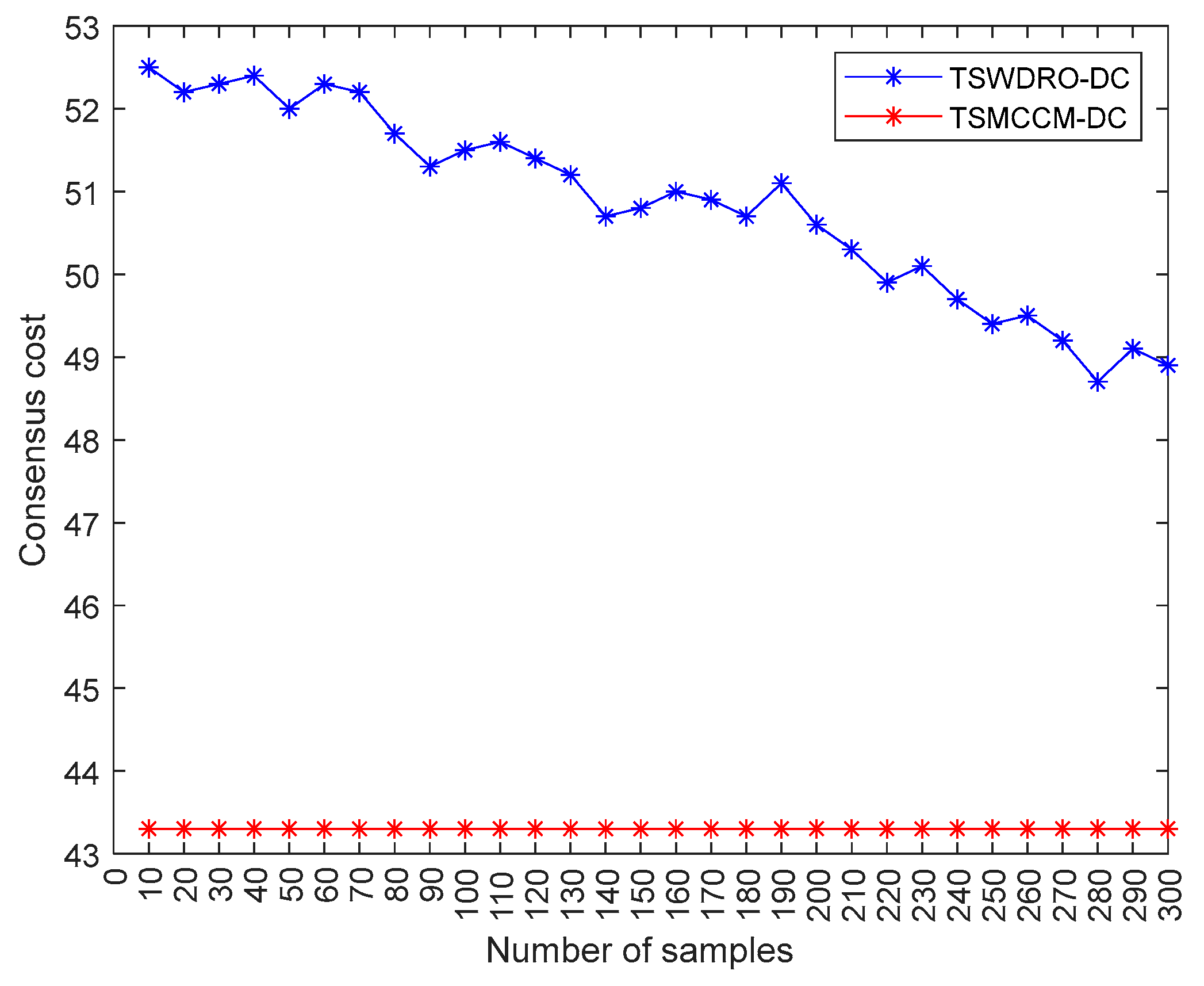
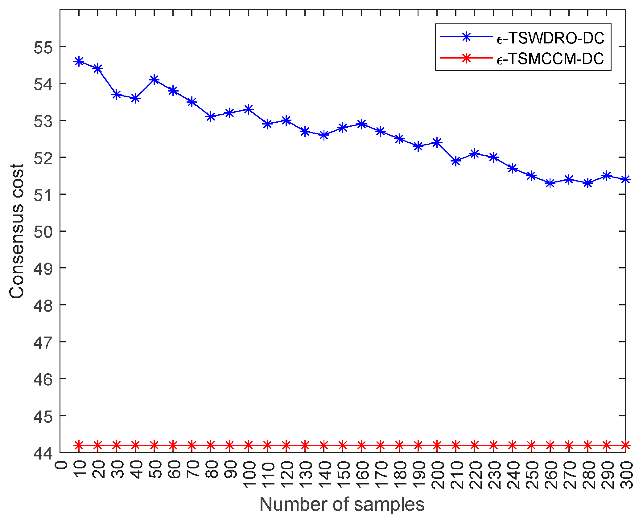
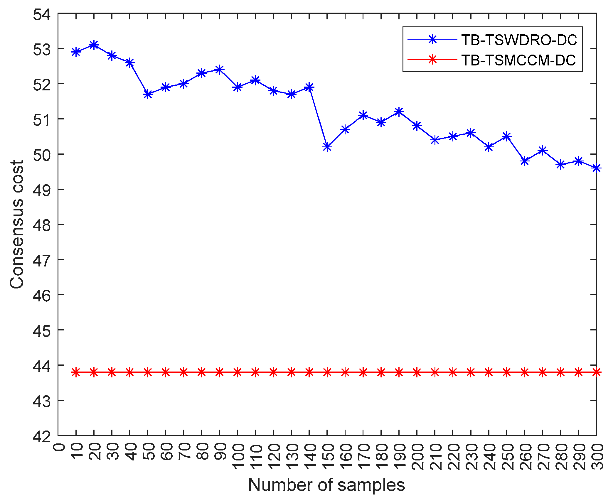
From Figure 1, Figure 2 and Figure 3, the fuzzy ensemble construction of TSWDRO-DC was influenced by the historical sample data and the results showed some volatility, reaching the optimal objective solution of 48.7 at a sample size of 280, while the result of TSMCCM-DC was constant at 43.3. Similarly, from Figure 2, at sample sizes of 260 and 280, the optimal result of 51.3 was reached by -TSMCCM-DC, where the result of 44.2 was reached using the deterministic approach. At a sample size of 300, the result of the TB-TSWDRO-DC model reached the optimal value of 49.6. Meanwhile, the result of the TB-TSMCCM-DC under the corresponding deterministic approach produced a value of 43.8. Although the cost value derived from the deterministic approach was smaller, the latter model was more conservative because it does not take the effect of risk uncertainty into account. From the perspective of the actual decision-making environment, the model proposed in this section was more consistent with the complex decision-making context, and the decision maker could flexibly choose different risk coefficients according to the current risk preference and obtain the corresponding decision results.
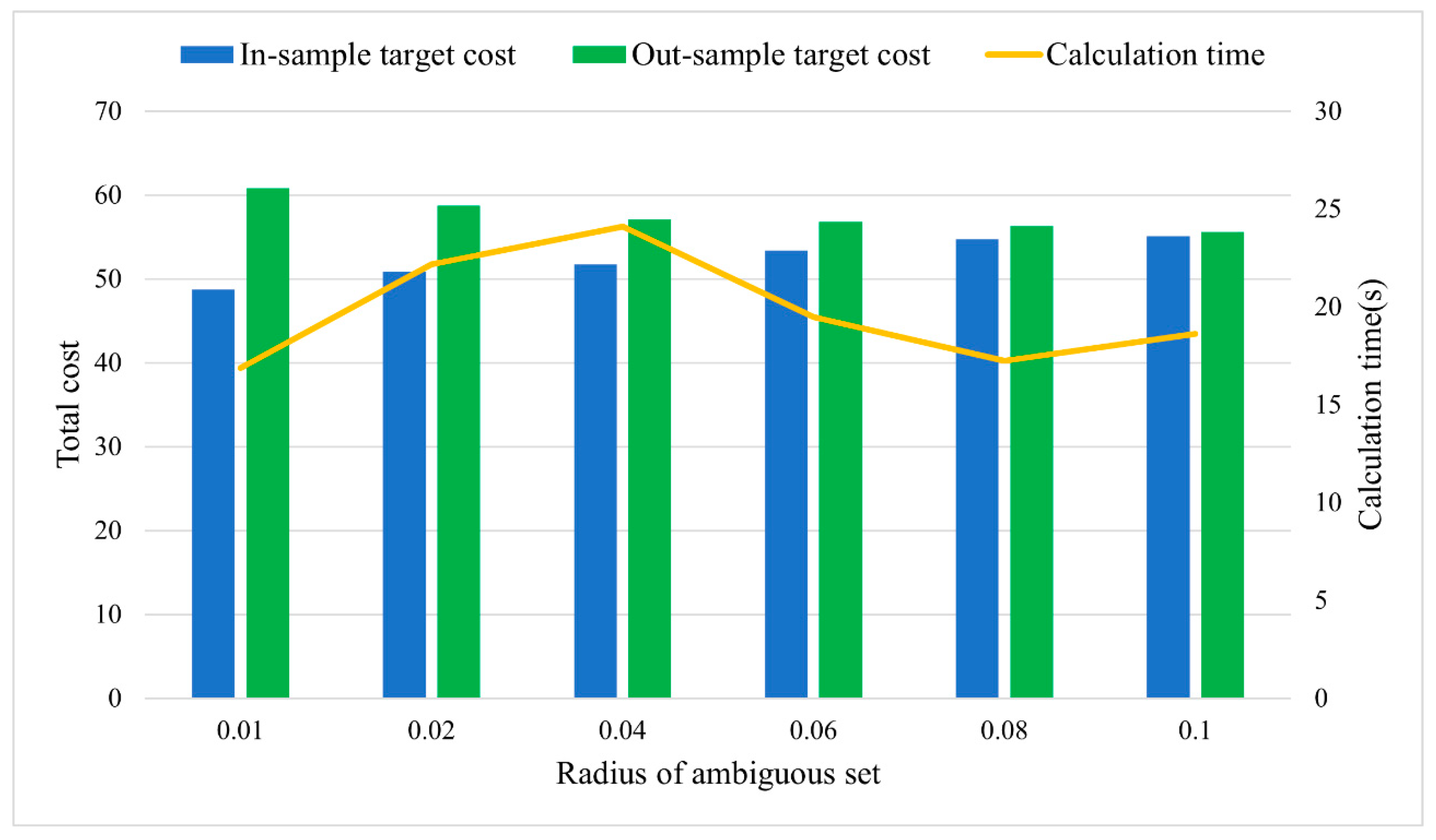
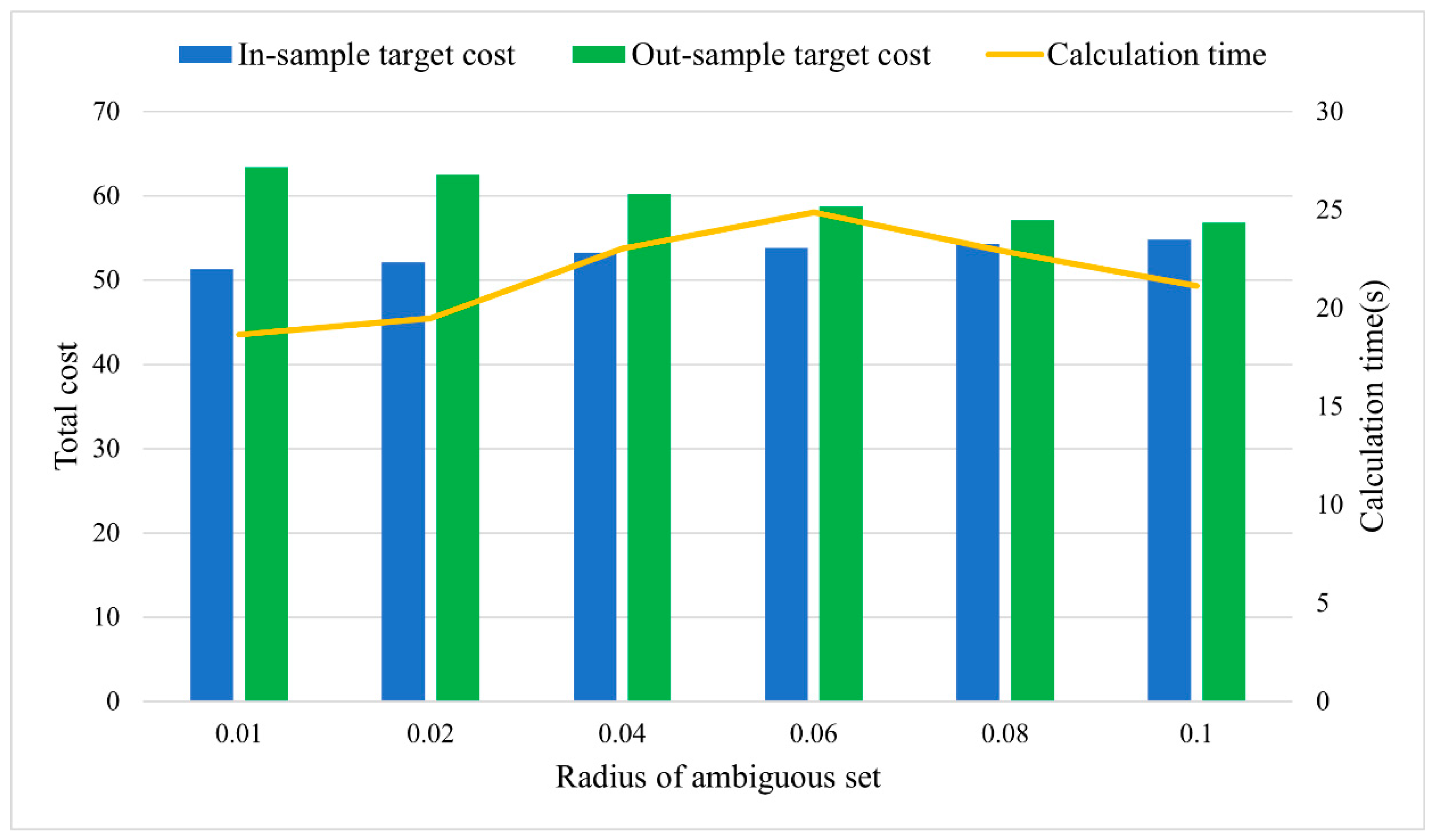
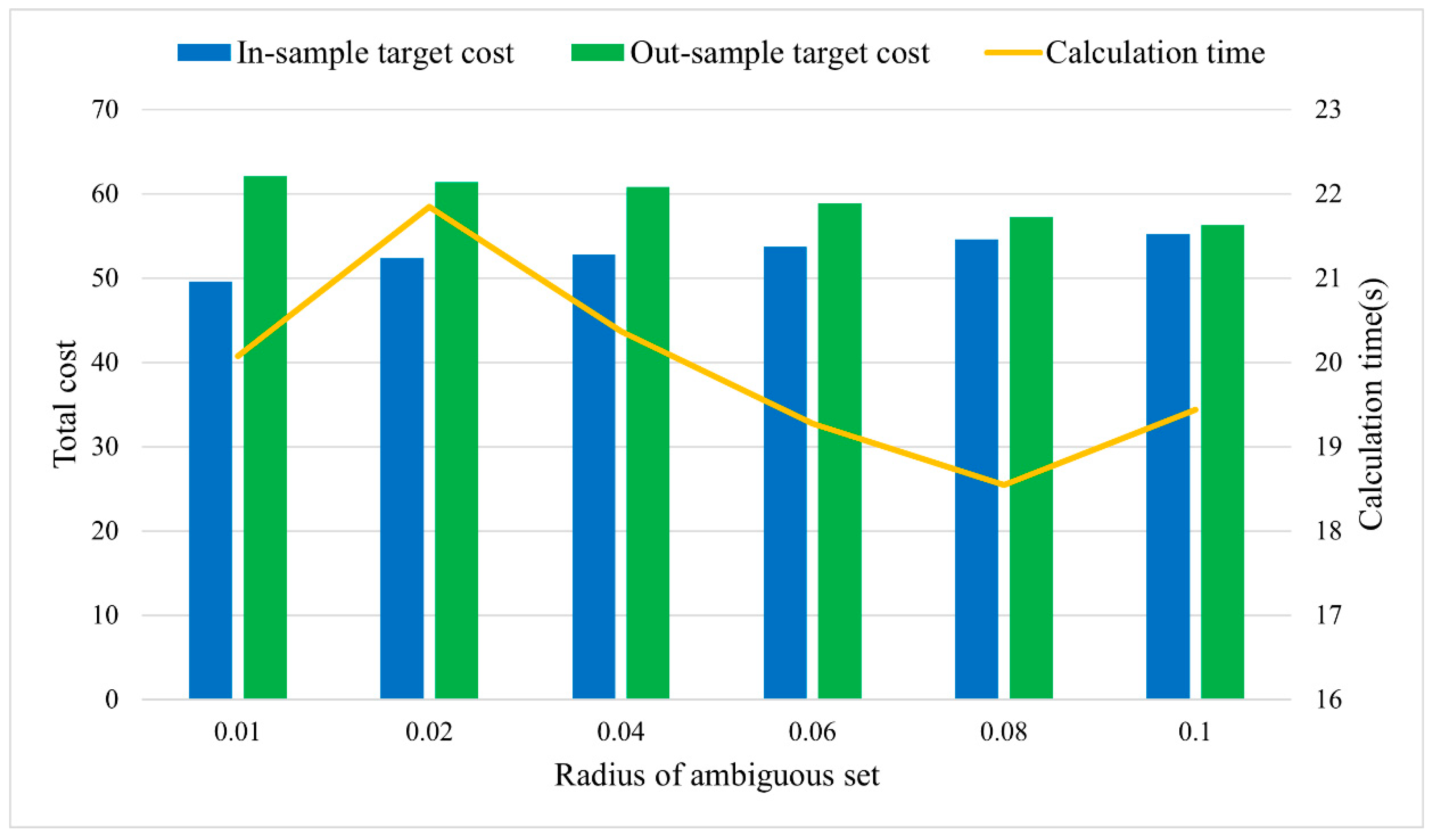
To further investigate how the in-sample performance, out-of-sample performance, and model solution time of the model varied with the radius of the Wasserstein ambiguous set in this section, a sensitivity analysis was performed. In Figure 4, Figure 5 and Figure 6, the results for different radius conditions are shown. The value of the radius specifies the size of the Wasserstein ambiguous set, and thus, the DMs can use it to adjust the conservativeness of the model. As mentioned above, as the radius increased, the ambiguous set encompassed more probability distributions, which meant that more distributions were hedged in the model. Since the model optimization in this section was about the worst-case expected cost of the ambiguous set, increasing the value of the ambiguous set radius led to a higher in-sample target cost, but the out-of-sample target cost decreased significantly initially and then stabilized. As can be seen from the orange line in the figure, increasing the radius of the Wasserstein ambiguous set did not significantly increase the computational burden, and the computational time to solve the corresponding problem fluctuated within a certain range.
5. Conclusions and Future Work
In this study, we proposed three new minimum-cost consensus models with asymmetric adjustment costs with the distributionally robust method. Then, a data-driven approach that utilized historical data was used to construct the Wasserstein ambiguous set with the Wasserstein distance as the basis of the metric. To simplify the calculation, three new models were transformed into a second-order cone programming problem. Then, taking the EU Trade and Animal Welfare (TAW) program policy consultation as an example, we carried out numerical simulations and compared the data with some existing models and the data were explained. Finally, some meaningful conclusions were obtained through numerical analysis:
- The change in the radius of the Wasserstein uncertainty sphere set had a significant impact on the consensus. As the radius increased, the target optimal cost became larger. The increase in radius meant that the ambiguous set covered more uncertainties. To overcome the effect of uncertainty, more cost was needed for the decision community to counteract the possible effects of consensus uncertainty. At the same time, this led to a more conservative model.
- Under the same initial settings, the optimal consensus cost in the three new models was higher than the deterministic models because the deterministic models did not consider the uncertainty effect and more cost was required to deal with the uncertainty. At the same time, the Wasserstein-metric-based distribution robust optimization approach was better than the robust optimization approach in the interval polyhedral uncertainty set for the TAW program policy consultation. The DRO method overcame the overly conservative results under the robust optimization approach and reflected the need for the study presented in this paper.
- The radius of the Wasserstein ambiguous set could be used to adjust the conservativeness of the models. As the radius increased, more probability distributions were contained in the ambiguous set, and thus, more distributions were hedged in the model.
- The models in this study considered the worst-case expected cost of the ambiguous set, where increasing the value of the ambiguous set radius led to a higher in-sample target cost, but the out-of-sample target cost decreased significantly initially and then stabilized.
To sum up, the proposed models better fit the complex decision context and yielded more realistic decision results. Although the proposed models expanded the MCCM to a certain extent, there were still some limitations in the real GDM. In the proposed models, besides the DMs’ opinions, the adjustment costs in different directions, the degree of tolerance, and the range of thresholds, other parameters can also impact the models, such as the DMs’ adjusted opinions. At the same time, the aggregation operators were not taken into account. In addition, only the Wasserstein ambiguous set was chosen in this study; this may lead to the models’ failure in other application scenarios.
Therefore, in the future, it is necessary to study the MCCM under different aggregation operators and more uncertain parameters should be considered with the DRO. Furthermore, it will be a very interesting research direction to extend the models proposed in this study to large-scale group decision-making. Finally, when the DRO method is used for research, a variety of different ambiguous sets can be selected, for example, the Wasserstein ambiguous set and -divergence, which will be meaningful in different applications.
Author Contributions
Conceptualization, Z.W.; methodology, Z.W.; software, Z.W.; validation, K.Z.; formal analysis, Z.W.; writing—original draft preparation, Z.W.; writing—review and editing, K.Z.; visualization, K.Z.; supervision, S.Q.; project administration, S.Q.; funding acquisition, S.Q. All authors have read and agreed to the published version of the manuscript.
Funding
This research received no external funding.
Institutional Review Board Statement
Not applicable.
Informed Consent Statement
Not applicable.
Data Availability Statement
The data is contained within the article.
Conflicts of Interest
The authors declare no conflict of interest.
References
- Wu, Z.; Xu, J. A concise consensus support model for group decision making with reciprocal preference relations based on deviation measures. Fuzzy Sets Syst. 2012, 206, 58–73. [Google Scholar] [CrossRef]
- Li, Y.; Chen, X.; Dong, Y.; Herrera, F. Linguistic group decision making: Axiomatic distance and minimum cost consensus. Inf. Sci. 2020, 541, 242–258. [Google Scholar] [CrossRef]
- Zhong, X.; Xu, X.; Pan, B. A non-threshold consensus model based on the minimum cost and maximum consensus-increasing for multi-attribute large group decision-making. Inf. Fusion 2022, 77, 90–106. [Google Scholar] [CrossRef]
- Wu, P.; Liu, J.; Zhou, L.; Chen, H. An Integrated Group Decision-Making Method with Hesitant Qualitative Information Based on DEA Cross-Efficiency and Priority Aggregation for Evaluating Factors Affecting a Resilient City. Group Decis. Negot. 2021, 31, 293–316. [Google Scholar] [CrossRef]
- He, Q.; Tong, H.; Liu, J.-B. How Does Inequality Affect the Residents’ Subjective Well-Being: Inequality of Opportunity and Inequality of Effort. Front. Psychol. 2022, 13, 843854. [Google Scholar] [CrossRef]
- Qu, S.; Xu, L.; Mangla, S.K.; Chan, F.T.S.; Zhu, J.; Arisian, S. Matchmaking in reward-based crowdfunding platforms: A hybrid machine learning approach. Int. J. Prod. Res. 2022, 1–21. [Google Scholar] [CrossRef]
- Zhang, X.; Ding, Z.; Hang, J.; He, Q. How do stock price indices absorb the COVID-19 pandemic shocks? N. Am. J. Econ. Financ. 2022, 60, 101672. [Google Scholar] [CrossRef]
- Priem, R.L.; Harrison, D.A.; Muir, N.K. Structured conflict and consensus outcomes in group decision making. J. Manag. 1995, 21, 691–710. [Google Scholar] [CrossRef]
- Palomares, I.; Martinez, L.; Herrera, F. A consensus model to detect and manage noncooperative behaviors in large-scale group decision making. IEEE Trans. Fuzzy Syst. 2013, 22, 516–530. [Google Scholar] [CrossRef]
- Mohammed, S.; Ringseis, E. Cognitive diversity and consensus in group decision making: The role of inputs, processes, and outcomes. Organ. Behav. Hum. Decis. Process. 2001, 85, 310–335. [Google Scholar] [CrossRef]
- Zhang, G.; Dong, Y.; Xu, Y.; Li, H. Minimum-Cost Consensus Models Under Aggregation Operators. IEEE Trans. Syst. Man Cybern. -Part A: Syst. Hum. 2011, 41, 1253–1261. [Google Scholar] [CrossRef]
- Ben-Arieh, D.; Easton, T. Multi-criteria group consensus under linear cost opinion elasticity. Decis. Support Syst. 2007, 43, 713–721. [Google Scholar] [CrossRef]
- Ben-Arieh, D.; Easton, T.; Evans, B. Minimum cost consensus with quadratic cost functions. IEEE Trans. Syst. Man Cybern. -Part A Syst. Hum. 2008, 39, 210–217. [Google Scholar] [CrossRef]
- Zhang, B.; Dong, Y.; Xu, Y. Maximum expert consensus models with linear cost function and aggregation operators. Comput. Ind. Eng. 2013, 66, 147–157. [Google Scholar] [CrossRef]
- Liang, Y.; Qin, J.; Martinez, L.; Liu, J. A heterogeneous QUALIFLEX method with criteria interaction for multi-criteria group decision making. Inf. Sci. 2020, 512, 1481–1502. [Google Scholar] [CrossRef]
- Xu, W.; Chen, X.; Dong, Y.; Chiclana, F. Impact of Decision Rules and Non-cooperative Behaviors on Minimum Consensus Cost in Group Decision Making. Group Decis. Negot. 2021, 30, 1239–1260. [Google Scholar] [CrossRef]
- Li, Y.; Ji, Y.; Qu, S. Consensus Building for Uncertain Large-Scale Group Decision-Making Based on the Clustering Algorithm and Robust Discrete Optimization. Group Decis. Negot. 2022, 31, 453–489. [Google Scholar] [CrossRef]
- Qin, J.; Li, M.; Liang, Y. Minimum cost consensus model for CRP-driven preference optimization analysis in large-scale group decision making using Louvain algorithm. Inf. Fusion 2022, 80, 121–136. [Google Scholar] [CrossRef]
- Cheng, D.; Zhou, Z.; Cheng, F.; Zhou, Y.; Xie, Y. Modeling the minimum cost consensus problem in an asymmetric costs context. Eur. J. Oper. Res. 2018, 270, 1122–1137. [Google Scholar] [CrossRef]
- Wei, J.; Qu, S.; Jiang, S.; Feng, C.; Xu, Y.; Zhao, X. Robust minimum cost consensus models with aggregation operators under individual opinion uncertainty. J. Intell. Fuzzy Syst. 2022, 42, 2435–2449. [Google Scholar] [CrossRef]
- Ma, G.; Zheng, J.; Wei, J.; Wang, S.; Han, Y. Robust optimization strategies for seller based on uncertainty sets in context of sequential auction. Appl. Math. Comput. 2021, 390, 125650. [Google Scholar] [CrossRef]
- Gong, Z.; Xu, X.; Guo, W.; Herrera-Viedma, E.; Cabrerizo, F.J. Minimum cost consensus modelling under various linear uncertain-constrained scenarios. Inf. Fusion 2021, 66, 1–17. [Google Scholar] [CrossRef]
- Ji, Y.; Li, H.; Zhang, H. Risk-Averse Two-Stage Stochastic Minimum Cost Consensus Models with Asymmetric Adjustment Cost. Group Decis. Negot. 2022, 31, 261–291. [Google Scholar] [CrossRef] [PubMed]
- Qu, S.; Li, Y.; Ji, Y. The mixed integer robust maximum expert consensus models for large-scale GDM under uncertainty circumstances. Appl. Soft Comput. 2021, 107, 107369. [Google Scholar] [CrossRef]
- Han, Y.; Qu, S.; Wu, Z.; Huang, R. Robust consensus models based on minimum cost with an application to marketing plan. J. Intell. Fuzzy Syst. 2019, 37, 5655–5668. [Google Scholar] [CrossRef]
- Qu, S.; Han, Y.; Wu, Z.; Raza, H. Consensus Modeling with Asymmetric Cost Based on Data-Driven Robust Optimization. Group Decis. Negot. 2020, 30, 1395–1432. [Google Scholar] [CrossRef]
- Jin, X.; Ji, Y.; Qu, S. Minimum cost strategic weight assignment for multiple attribute decision-making problem using robust optimization approach. Comput. Appl. Math. 2021, 40, 193. [Google Scholar] [CrossRef]
- Li, H.; Ji, Y.; Gong, Z.; Qu, S. Two-stage stochastic minimum cost consensus models with asymmetric adjustment costs. Inf. Fusion 2021, 71, 77–96. [Google Scholar] [CrossRef]
- Delage, E.H. Distributionally Robust Optimization in Context of Data-Driven Problems; Stanford University: Stanford, CA, USA, 2009. [Google Scholar]
- Delage, E.; Ye, Y. Distributionally robust optimization under moment uncertainty with application to data-driven problems. Oper. Res. 2010, 58, 595–612. [Google Scholar] [CrossRef] [Green Version]
- Yang, Y.; Wu, W. A Distributionally Robust Optimization Model for Real-Time Power Dispatch in Distribution Networks. IEEE Trans. Smart Grid 2018, 10, 3743–3752. [Google Scholar] [CrossRef]
- Han, Y.; Qu, S.; Wu, Z. Distributionally Robust Chance Constrained Optimization Model for the Minimum Cost Consensus. Int. J. Fuzzy Syst. 2020, 22, 2041–2054. [Google Scholar] [CrossRef]
- Huang, R.; Qu, S.; Yang, X.; Liu, Z. Multi-stage distributionally robust optimization with risk aversion. J. Ind. Manag. Optim. 2021, 17, 233–259. [Google Scholar] [CrossRef] [Green Version]
- Wang, W.; Yang, K.; Yang, L.; Gao, Z. Two-stage distributionally robust programming based on worst-case mean-CVaR criterion and application to disaster relief management. Transp. Res. Part E: Logist. Transp. Rev. 2021, 149, 102332. [Google Scholar] [CrossRef]
- Bertsimas, D.; Sim, M.; Zhang, M. Adaptive Distributionally Robust Optimization. Manag. Sci. 2019, 65, 604–618. [Google Scholar] [CrossRef] [Green Version]
- Cuesta, J.A.; Matrán, C. Notes on the Wasserstein metric in Hilbert spaces. Ann. Probab. 1989, 17, 1264–1276. [Google Scholar] [CrossRef]
Figure 1.
Comparison of the TSWDRO-DC and TSMCCM-DC results.

Figure 2.
Comparison of the -TSWDRO-DC and -TSMCCM-DC results.

Figure 3.
Comparison of the TB-TSWDRO-DC and TB-TSMCCM-DC results.

Figure 4.
Sensitivity analysis of TSWDRO-DC.

Figure 5.
Sensitivity analysis of -TSWDRO-DC.

Figure 6.
Sensitivity analysis of TB-TSWDRO-DC.


Table 1.
Information data related to the DMs in the model.
| Initial Decision-Making Comments | Experience Cost Factor | Experience Cost Factor | Threshold | Adjustment Range | |
|---|---|---|---|---|---|
| 1 | 5.7 | 11 | 13 | 24 | 3 |
| 2 | 6.3 | 16 | 14 | 22 | 6 |
| 3 | 4.9 | 12 | 15 | 18 | 5 |
| 4 | 5.3 | 13 | 14 | 21 | 2 |
| 5 | 2.8 | 9 | 15 | 15 | 4 |
| 6 | 3.2 | 10 | 11 | 16 | 7 |
| 7 | 4.5 | 14 | 11 | 25 | 3 |
| 8 | 6.8 | 15 | 13 | 18 | 8 |
| 9 | 7.1 | 18 | 14 | 20 | 6 |
| 10 | 3.6 | 10 | 15 | 22 | 4 |
Table 2.
Numerical simulation results.
| Models | Consensus Cost | Models | Consensus Cost | ||
|---|---|---|---|---|---|
| 0.01 | TSWDRO-DC | 48.7 | 0.02 | TSWDRO-DC | 50.9 |
| -TSWDRO-DC | 51.3 | -TSWDRO-DC | 52.1 | ||
| TB-TSWDRO-DC | 49.6 | TB-TSWDRO-DC | 52.4 | ||
| 0.04 | TSWDRO-DC | 51.7 | 0.06 | TSWDRO-DC | 53.4 |
| -TSWDRO-DC | 53.2 | -TSWDRO-DC | 53.8 | ||
| TB-TSWDRO-DC | 52.8 | TB-TSWDRO-DC | 53.7 | ||
| 0.08 | TSWDRO-DC | 54.7 | 0.1 | TSWDRO-DC | 55.1 |
| -TSWDRO-DC | 54.3 | -TSWDRO-DC | 54.8 | ||
| TB-TSWDRO-DC | 54.6 | TB-TSWDRO-DC | 55.2 |
Table 3.
Comparison of optimal results of different cost consensus models.
| Categorization | Models | Consensus Opinion | Optimal Consensus Cost |
|---|---|---|---|
| Deterministic approach | TSMCCM-DC | 5.8 | 43.3 |
| -TSMCCM-DC | 5.6 | 44.2 | |
| TB-TSMCCM-DC | 5.9 | 43.8 | |
| Methodology of this article | TSWDRO-DC | 5.7 | 48.7 |
| -TSWDRO-DC | 5.8 | 51.3 | |
| TB-TSWDRO-DC | 5.8 | 49.6 |
Table 4.
Comparison of optimal results of different cost consensus models.
| Categorization | Models | Ambiguous Set/Uncertain Set | Optimal Consensus Cost |
|---|---|---|---|
| Robust optimization methods | TSMCCM-DC | Box set | 53.2 |
| Ellipsoid set | 53.1 | ||
| Polyhedral set | 52.8 | ||
| Interval-polyhedral set | 51.6 | ||
| -TSMCCM-DC | Box set | 55.7 | |
| Ellipsoid set | 56.9 | ||
| Polyhedral set | 53.4 | ||
| Interval-polyhedral set | 53.9 | ||
| TSMCCM-DC | Box set | 54.8 | |
| Ellipsoid set | 52.6 | ||
| Polyhedral set | 53.1 | ||
| Interval-polyhedral set | 52.5 | ||
| Methodology of this article | TSWDRO-DC | Wasserstein ambiguous sets | 48.7 |
| -TSWDRO-DC | 51.3 | ||
| TB-TSWDRO-DC | 49.6 |
Publisher’s Note: MDPI stays neutral with regard to jurisdictional claims in published maps and institutional affiliations. |
© 2022 by the authors. Licensee MDPI, Basel, Switzerland. This article is an open access article distributed under the terms and conditions of the Creative Commons Attribution (CC BY) license (https://creativecommons.org/licenses/by/4.0/).
Share and Cite
MDPI and ACS Style
Wu, Z.; Zhu, K.; Qu, S. Distributionally Robust Optimization Model for a Minimum Cost Consensus with Asymmetric Adjustment Costs Based on the Wasserstein Metric. Mathematics 2022, 10, 4312. https://doi.org/10.3390/math10224312
AMA Style
Wu Z, Zhu K, Qu S. Distributionally Robust Optimization Model for a Minimum Cost Consensus with Asymmetric Adjustment Costs Based on the Wasserstein Metric. Mathematics. 2022; 10(22):4312. https://doi.org/10.3390/math10224312
Chicago/Turabian StyleWu, Ziqi, Kai Zhu, and Shaojian Qu. 2022. "Distributionally Robust Optimization Model for a Minimum Cost Consensus with Asymmetric Adjustment Costs Based on the Wasserstein Metric" Mathematics 10, no. 22: 4312. https://doi.org/10.3390/math10224312
Note that from the first issue of 2016, this journal uses article numbers instead of page numbers. See further details here.