


Increasing the Effectiveness of Network Intrusion Detection Systems (NIDSs) by Using Multiplex Networks and Visibility Graphs

1
Data, Complex Networks and Cybersecurity Sciences Technological Institute, University Rey Juan Carlos, 28028 Madrid, Spain
2
Departamento de Matemática Aplicada, Ciencia e Ingeniería de los Materiales y Tecnología Electrónica, ESCET Universidad Rey Juan Carlos, C/Tulipán s/n, 28933 Mostoles, Spain
3
Center for Computational Simulation, Universidad Politécnica de Madrid, 28223 Madrid, Spain
*
Authors to whom correspondence should be addressed.
Mathematics 2023, 11(1), 107; https://doi.org/10.3390/math11010107
Submission received: 26 October 2022
/
Revised: 24 November 2022
/
Accepted: 30 November 2022
/
Published: 26 December 2022
(This article belongs to the Special Issue Mathematical Models in Security, Defense, Cyber Security and Cyber Defense II)
Abstract
:In this paper, we present a new approach to NIDS deployment based on machine learning. This new approach is based on detecting attackers by analyzing the relationship between computers over time. The basic idea that we rely on is that the behaviors of attackers’ computers are different from those of other computers, because the timings and durations of their connections are different and therefore easy to detect. This approach does not analyze each network packet statistically. It analyzes, over a period of time, all traffic to obtain temporal behaviors and to determine if the IP is an attacker instead of that packet. IP behavior analysis reduces drastically the number of alerts generated. Our approach collects all interactions between computers, transforms them into time series, classifies them, and assembles them into a complex temporal behavioral network. This process results in the complex characteristics of each computer that allow us to detect which are the attackers’ addresses. To reduce the computational efforts of previous approaches, we propose to use visibility graphs instead of other time series classification methods, based on signal processing techniques. This new approach, in contrast to previous approaches, uses visibility graphs and reduces the computational time for time series classification. However, the accuracy of the model is maintained.
1. Introduction
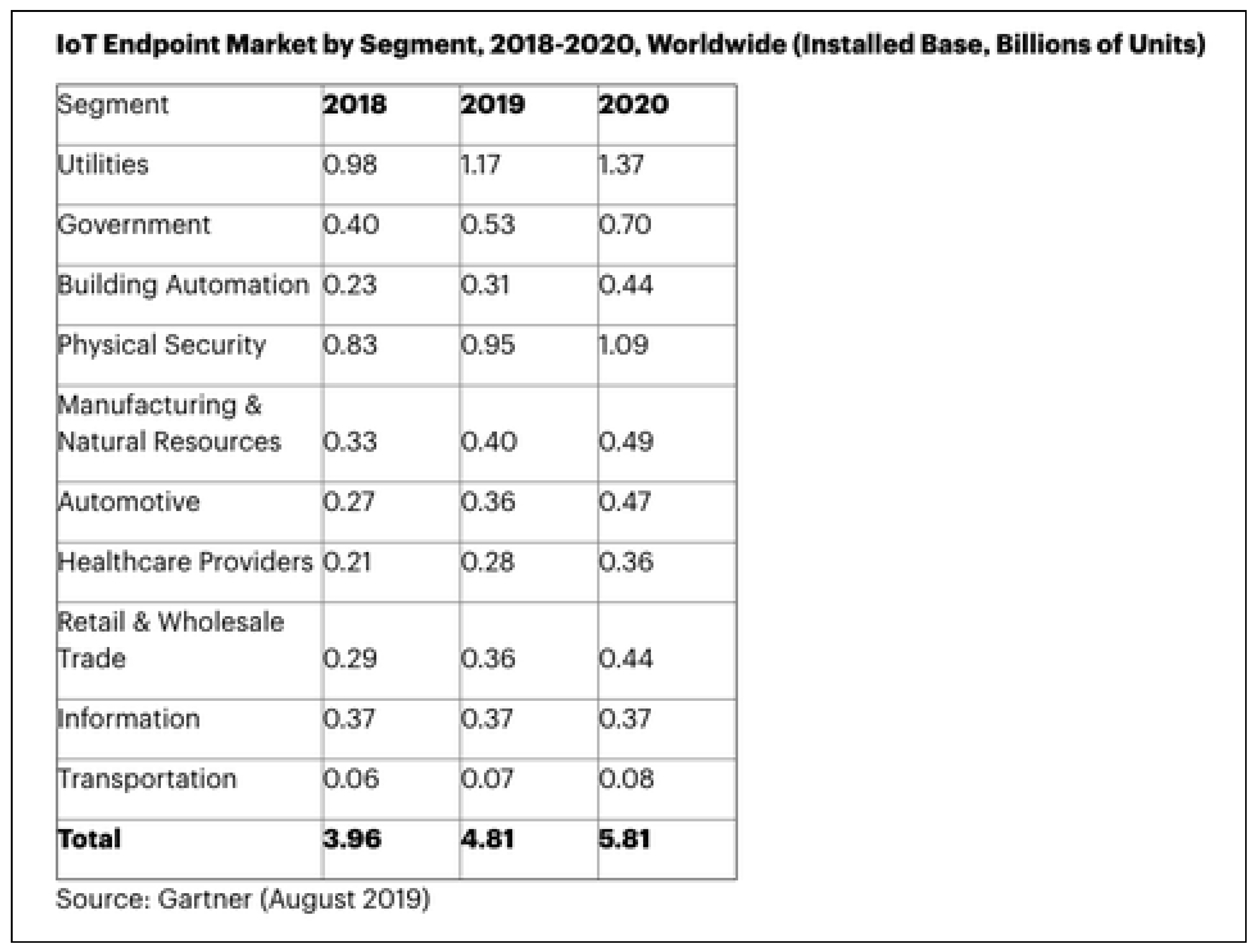
Nowadays, the amount of worldwide information among connected devices is growing exponentially. This growth provides us with a field where the availability of information in an adequate form provides a huge differential for the detection of appropriate shreds of evidence within an increasing amount of data. IoT is one of the most important disciplines where this increase happens. Gartner, the world’s leading research and advisory company, predicts a great amount of interconnected IoT endpoints. Cybersecurity must answer the requirements stemming from this increase in new devices. Network modeling provides a conceptual framework for describing the the relationships between systems and measures them in a meaningful way [1,2,3,4,5]. During the last two decades, a branch of science was born; it was known as complex network theory. This science has a main goal of exploiting the current availability of big data to extract a representation of the underlying complex systems and mechanisms [6,7,8,9,10,11,12,13]. Complex network theory tries to explore complex systems to find new forms to analyze them [14,15,16]. In the model, a complex network is used to represent the scenario, where the nodes are the different components of the system, while the edges represent the links between them. So, the attacker navigates through the computer network to extract and to capture valuable information contained in the system. Each hop from one node to another has its own cost, depending on the ease of accessing a new computer. In any case, this myriad of IoT endpoints (5.81 billion units of new IoT devices as describe in Figure 1) requires effective cybersecurity processes.
Cybersecurity is one of the disciplines that has grown the most in recent years, trying to cover new needs arising in the new digital environments and the IoT of large corporations. In the United States, cybercrime costs businesses more than $3.5 billion a year in Internet-related crimes and damages, according to a 2019 FBI report. The increasing number of computers and endpoints connected to the Internet renders a more complex playground to detect attackers. These losses show the real need to improve detection, protection, and reaction tools in large corporations where the current solutions don’t solve their real security needs. Cybersecurity spending will reach up to $123 B in 2020, and the security and risk management of cybersecurity is predicted to grow to 2.4%, down from a projected growth rate at the beginning of this year of 8.7%, according to Gartner’s security and risk management spending forecast.
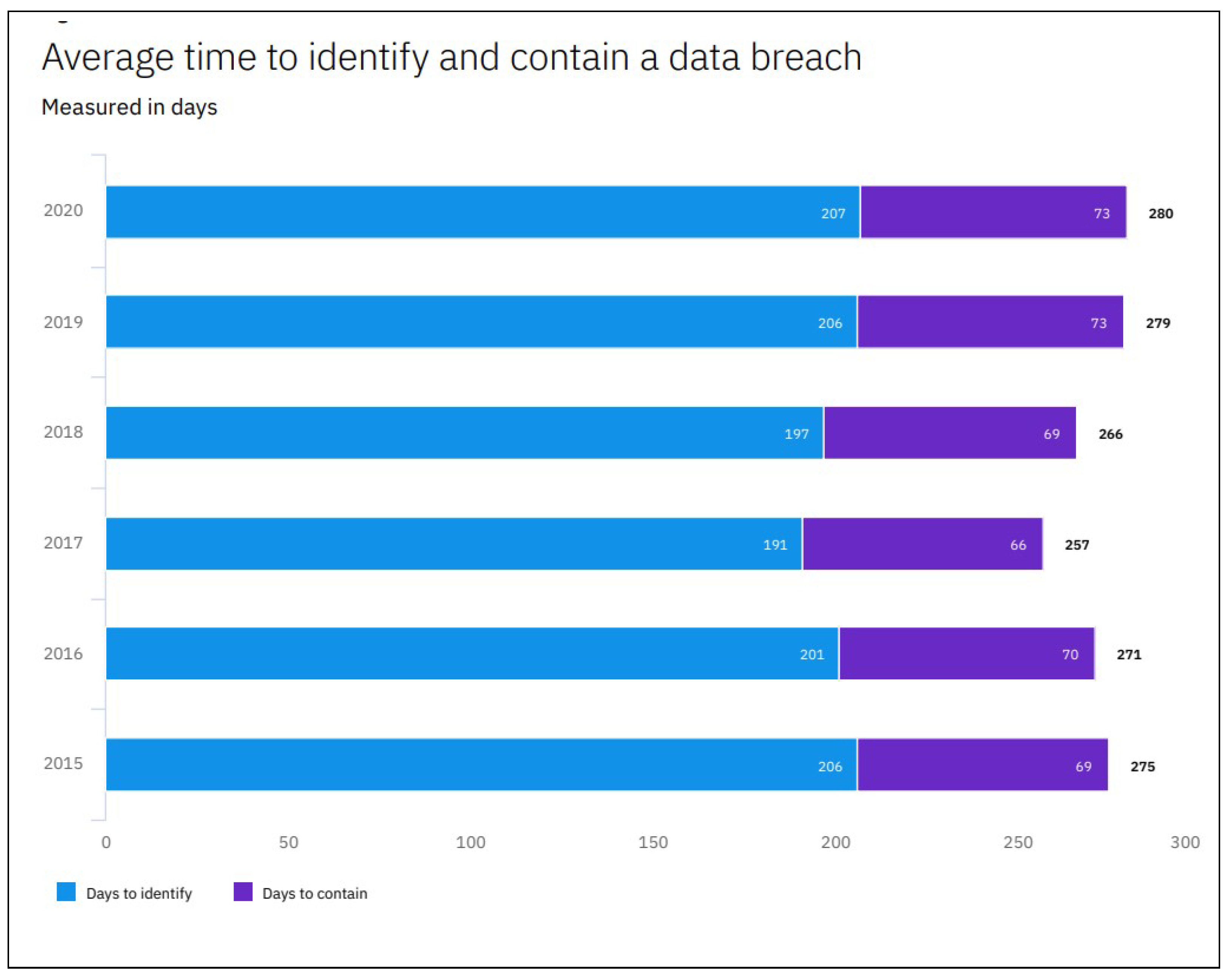
In this situation, one of the most important challenges is to detect any security gap inside the network as soon as possible. One of the most commonly used indicators to measure the time spent for SOC analysts to detect an attacker in the network is called MTTD (Mean Time to Detection). However, the evolution of the MTTD is increasing in recent years, as Cost of a Data Breach Report 2020 describes (https://www.ibm.com/security/digital-assets/cost-data-breach-report/, access on 20 September 2022). The actual trend is that the MTTD is increasing to 207 days over the last few years, as we can see in Figure 2.
To reduce this indicator, a large number of security arrangements are deployed in the networks. One of them is the NIDS. The Network Intrusion Detection System can be described as a device, a software application that monitors a network or computer for malicious activity or policy violations. NIDS inspects every network packet and payloads against a huge number of rules. These rules usually find some payload flag or information, similar to an antivirus, detecting some attack pattern, as we can see in the examples described in Listing 1. Every rule is made by inspecting every packet generated in an attack and finding some characteristic behavior, and so it must be developed by security analyst experts located in 24 × 7 security labs. After development, these rules are sent to large corporations using subscription services that update the ruleset periodically to detect new attack patterns.
| Listing 1. snort NIDS rule examples. |
| alert tcp $EXTERNAL_NET any -> $TELNET_SERVERS 23 \ ( msg:"MALWARE-BACKDOOR␣w00w00␣attempt"; flow:to_server,established; content:"w00w00"; metadata:ruleset community; classtype:attempted-admin; sid:209; rev:9; ) alert tcp $EXTERNAL_NET any -> $TELNET_SERVERS 23 \ ( msg:"MALWARE-BACKDOOR␣attempt"; flow:to_server,established; content:"backdoor",nocase; metadata:ruleset \ community; classtype:attempted-admin; sid:210; rev:7; ) alert tcp $EXTERNAL_NET any -> $TELNET_SERVERS 23 \ ( msg:"MALWARE-BACKDOOR␣MISC␣r00t␣attempt"; \ flow:to_server,established; content:"r00t"; metadata:ruleset community; classtype:attempted-admin; sid:211; rev:7; ) alert tcp $EXTERNAL_NET any -> $TELNET_SERVERS 23 \ ( msg:"MALWARE-BACKDOOR␣MISC␣rewt␣attempt"; flow:to_server,established; content:"rewt"; metadata:ruleset community; classtype:attempted-admin; sid:212; rev:7; ) |
This ruleset creation has three main disadvantages:
- No zero-day attacks detection,
- Lots of false positive alerts because the rule only finds limited patterns in the packets,
- No contextual information about generated alerts
Because any generated alert must be analyzed to detect attackers in large corporations, any intrusion activity or violation is typically reported to an administrator or is collected centrally using another cybersecurity tool called Security Information and Event Management (SIEM). SIEM tries to reduce one of the disadvantages of NIDS and other cybersecurity tools, and the contextual information, focusing on the correlation of existing information within the generated alerts, giving the SOC analyst more information about the environment where the alert was triggered. SIEM combines outputs from multiple sources and uses alarm filtering techniques to distinguish malicious activity from false alarms. These early detection systems need to send the least number of alarms possible to the SOC cybersecurity team. A large number of false positives can reduce the effectiveness of an entire cybersecurity department by focusing on non-critical investigations. Therefore, an actual approach of inspecting every network packet, focusing only on the payload of the packet and the network session information, is not enough to reduce the MTTD metric.
In this paper, our challenge is to reduce the number of days for the detection, focusing on the behavior of the network-connected device, rather than evaluating every networking event separately, because individual events don’t help us to detect them in the early stages of the attacks.
We therefore present an approach that provides us with the benefits of both techniques (time series and networks) by generating a graph that is contextualized with the information extracted from the communications behavior detailed using UEBA techniques (User Entity and Behavior Analytics).
To achieve this, we propose a new technique to develop NIDSs to focus on IP address behavior, instead of focusing on a single network packet. Using temporal behavior multiplex networks, we can obtain the behavior of each computer and find anomaly computers, generating alerts. In this paper, we use visibility graphs and Kmeans for clustering time series quicker than previous research.
2. Materials and Methods
This section is devoted to presenting our new approach, taking as a starting point the methodology developed in [17,18]. First, we suggest a possible NIDS architecture that can be used to deploy this NIDS. Second, we describe the dataset that we use to validate our method. Third, we describe, step-by-step, how we create and use the multiplex temporal behavioral network with a new visibility graph-based approach. Finally, we present the results.
3. Machine Learning Based on Intrusion Detection Systems
Nowadays, intrusion detection systems’ most important challenge is to increase their accuracy in more complex networks, with more computers and more communications taking place. As attack techniques become more sophisticated and more extended in time, the meantime to detect the attacker increases due to the difficulty of filtering false positive alarms from the real alerts generated for the attacker’s activity.
The most common type of NIDS is based on ruleset and protocol violation techniques. There are also new approaches based on machine learning techniques to identify attacker events. These new approaches try to solve two of the disadvantages of NIDSs: zero-day attack detection and false-positive reduction in large corporations trying to give the SOC analyst more accurate alerts to detect any attack in the early stages.
3.1. Related Works
There are many ways to analyze the network packet within the machine learning, based on intrusion detection systems. We can find several approaches based on each machine learning technique discovered.
At a first step, we can split them according to how many algorithms are used. Most common approach is to use only one algorithm. However, there are ones using a combination of algorithms [19,20].
In summary, we can reduce all the techniques in:
- Pattern classifiers;
- Single classifiers: K-nearest neighbor, support vector machines, artificial neural networks, etc.;
- Hybrid classifiers;
- Ensemble classifiers.
In addition to these techniques, in recent years, several new techniques have appeared, such as reinforcement learning [21] or Convolutional LSTM Networks [22] or deep learning [23,24,25]. Other techniques are based on time series, such as [26,27,28], as well as complex networks [29,30]. However, none of these approaches have provided a unique solution to this problem.
Generally speaking, any supervised or unsupervised technique is valid for use in developing an NIDS.
However, all of these approaches are focusing on the same target: find the best accuracy in the model. There is no different approach between them.
In our case, we propose a deeper technique to acquire the behavioral information.
To meet the challenge, we have relied on defining patterns of computer behavior through a temporal behavior multiplex network, and then looking for combinations that are unusual for attacker detection. There are other approaches, such as link prediction [31], which could be equally interesting for the detection of unusual computer behavior. Both approaches are complementary and could be a field for further research.
3.2. NIDS Architecture
We propose a new method for alert generation. An actual NIDS checks every network packet with a ruleset or machine learning algorithm; our approach collects network traffic in a period. After collecting all of this information, it activates alerts with the possible attacker IP addresses in the period. In Figure 3, we show the basic architecture for collecting network traffic and from it, triggering alerts.
With this approach, we take more information about the behaviors of the computers, rather than checking every network packet at the same time.
3.3. Dataset
The first challenge of most real cases is that the data arranged in log files that store the information sequentially. These files have little information on each event, so their aggregation into a network will allow us to obtain a greater amount of information.
As we have to create time series from the interactions between each IP address, it is necessary, for this technique to be used, there must be enough events that are relevant to each IP address.
One of the biggest challenges is to find a dataset that lets us compare our ideas with the ideas that are published in other papers. For this purpose, we have decided to use a dataset that is well known in the field of intrusion detection systems. In our case, we are going to use the Bot-IoT dataset [32] because it meets the requirements we need for our approach:
- A dataset format based on network flows and their features,
- Long-term monitoring: to understand the the behavior of every network communication, we need information over time,
- A labeled dataset,
- Wide usage in previous research to be compared with.
This dataset fulfils all our requirements:
- It collects every flow from a network. The dataset contains more than 72,000,000 records;
- It labels which communication is an attack;
- It provides us with a great number of features describing it from every network flow between two IP address, as we can see in Table 1.
In addition, we must not forget that this a reference for the evaluation of IDS.
3.4. Temporal Behavior Multiplex Network
In this paper, we propose an improved approach to creating a multiplex network of temporal behavior to forecast any time-based use case, based on the earlier published technique proposed in previous papers [17,18]. However, this new approach uses a different technique to acquire the temporal behaviors of the assets. In this case, we propose to use visibility graphs.
The main reason for modifying the technique proposed in a previous paper is to find more accuracy and less computational effort in optimizing the previously proposed technique, as we will discuss below.
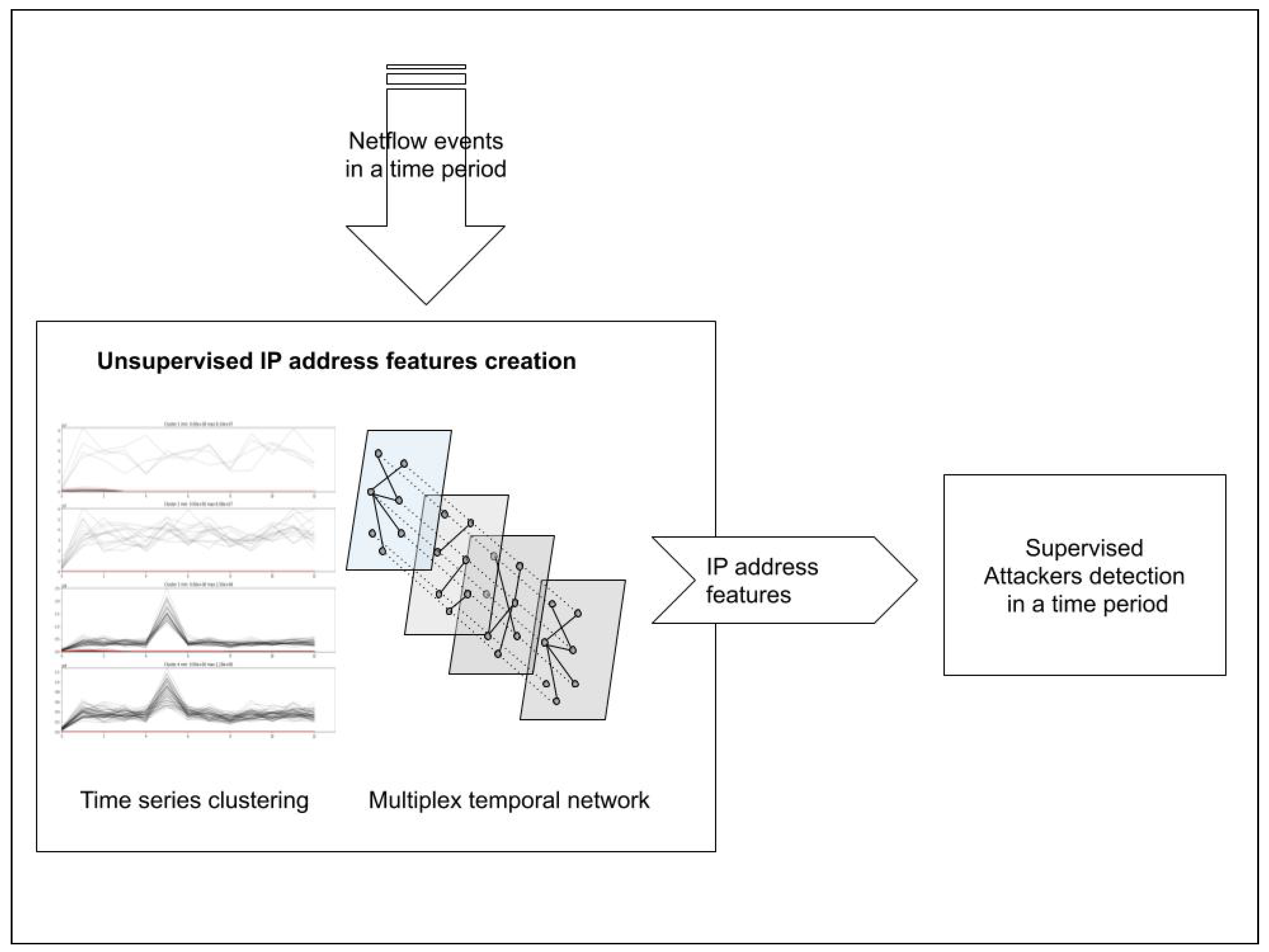
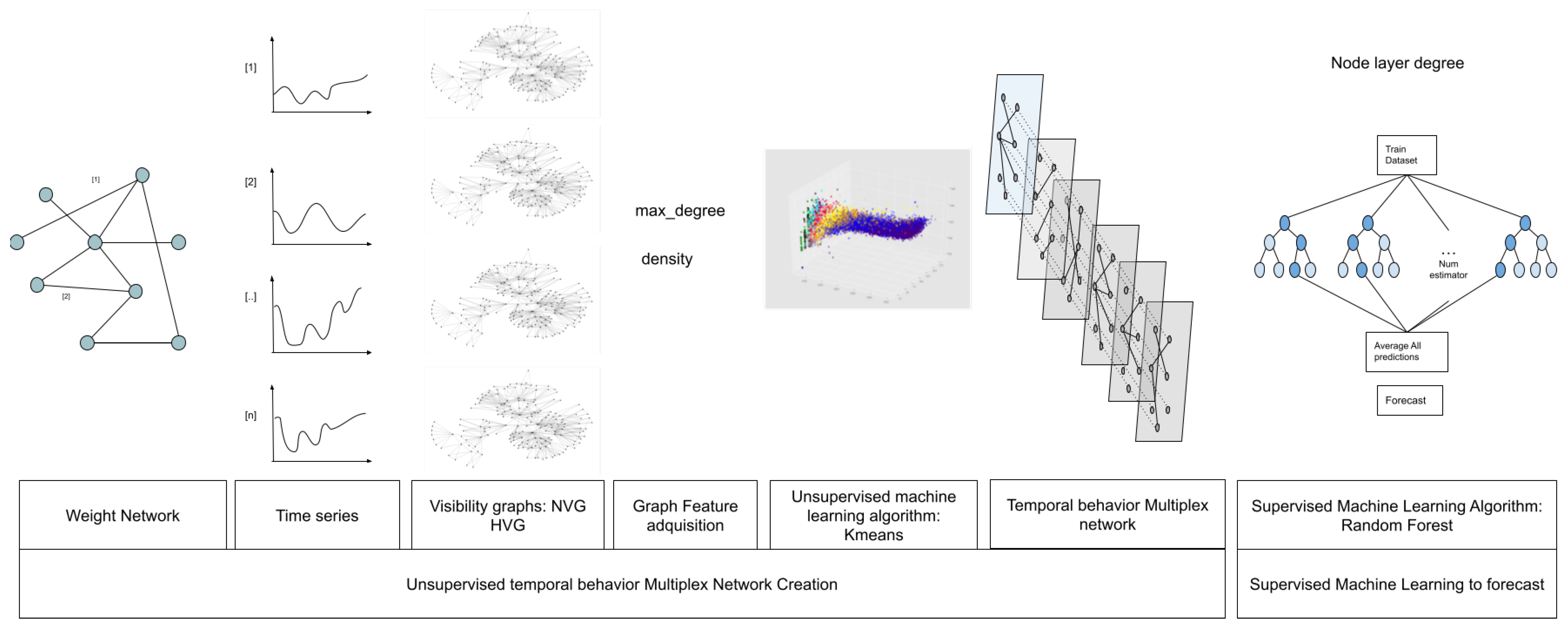
We follow the same workflow described before in the previous research Figure 4. First of all, we have to collect all of the network packet information inside the temporal behavior multiplex network, and after this, to extract complex features from the network to predict if an IP address is an attacker or not, using a controlled machine learning algorithm. However, in this new approach, we propose to use the visibility graphs, Kmeans to time series classification, instead of the KShape algorithm.
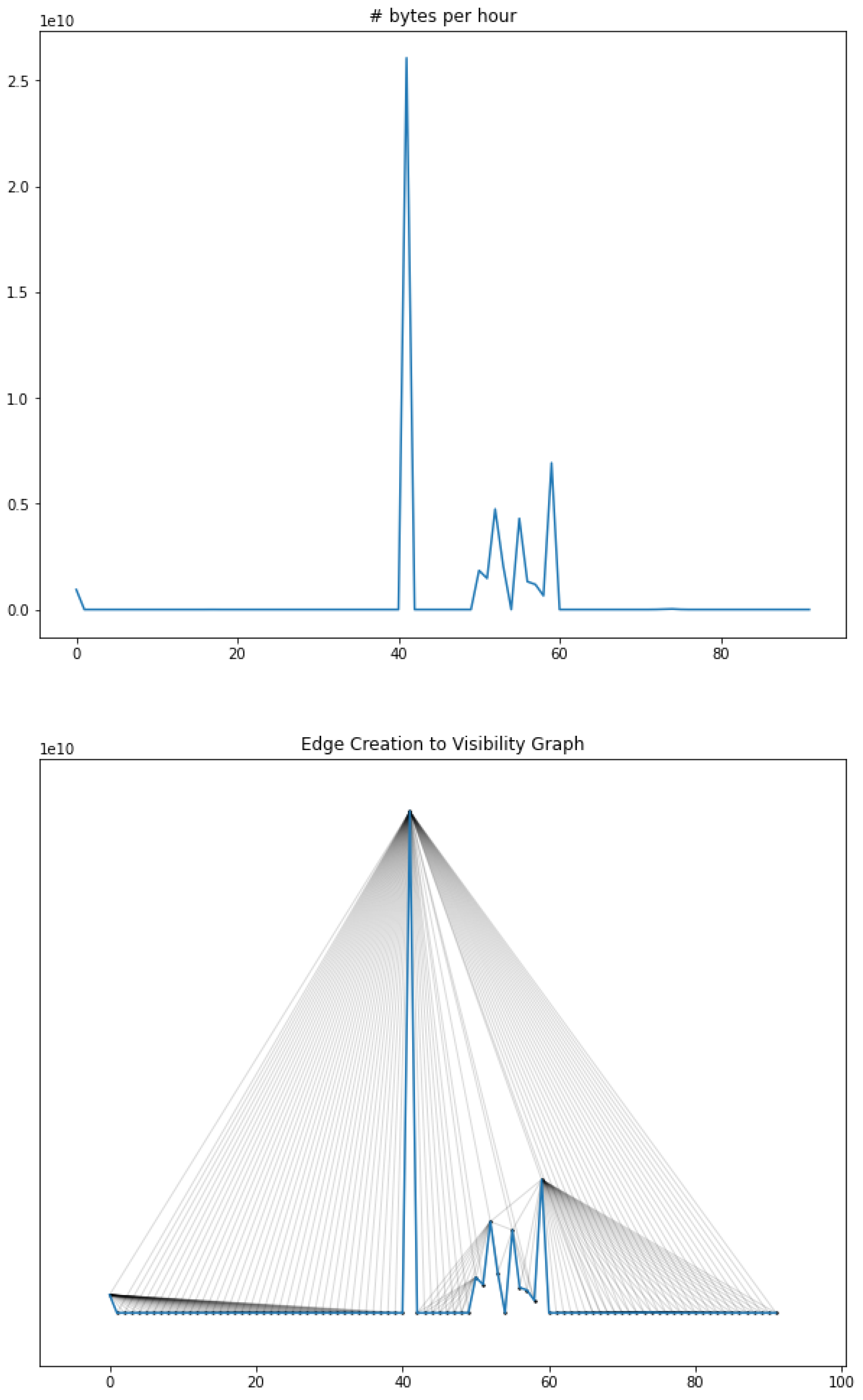
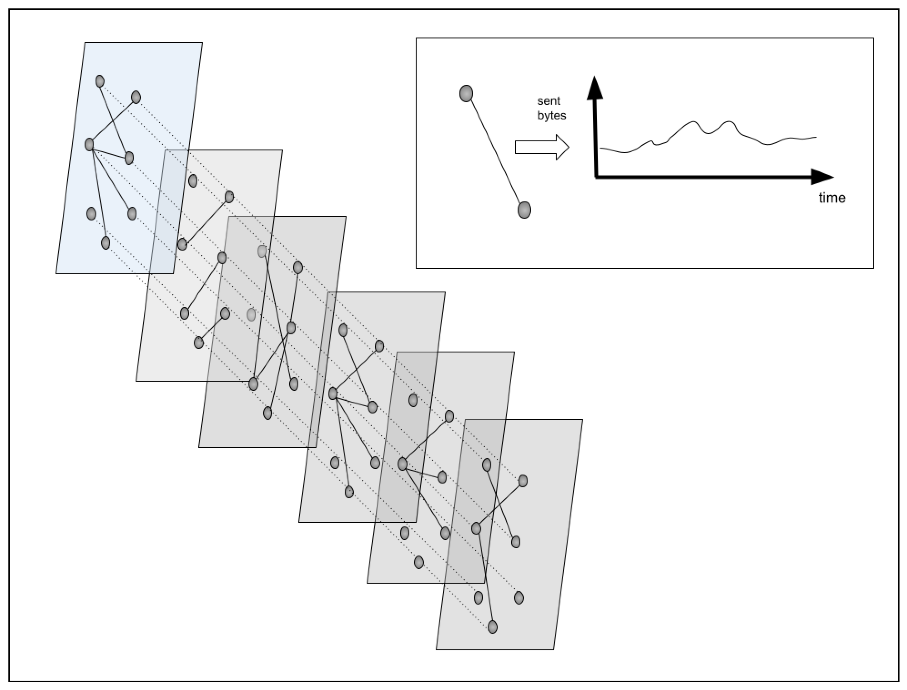
To create the temporal behavior multiplex network, first of all, we create a time series, collecting the iterations between two nodes. This time series gives us information about the evolution over time of the relation between them, using the number of bytes per hour as a slot, as we can see in the first part of Figure 5.
The second step consists in creating a classification of these times series. For this purpose, we decide to use a combination of visibility graphs and the Kmeans unsupervised algorithm. With this, we create time series clusters. Each cluster describes a similar relationship between two computers.
The final step is to fill the multiplex network. This multiplex network will have many layers as clusters of the time series we have. Each edge connecting two computers will be placed in the layer, depending on the cluster of the time series created from the information of the edge. For example, if the time series created with the bytes per hour between two computers is located in cluster #5, the edge between these two nodes will be placed in layer #5 of the multiplex network.
The ultimate goal of the creation of this multiplex network is to put it together in the same layer with similar traffic patterns. That is, all computers trying to surf the Internet will be located in the same layer. Each node will have edges in one or more layers describing its relationship with the rest of the network.
The first item is to collect all temporal information about the relationship between the assets inside a temporal behavior complex network. We describe in the following paragraphs how to create it.
First of all, we consider a weighted network as a single layer network defined using the form
where N is defined as a set of nodes and E the set of edges connecting the nodes as , and W is defined as the weight of every edge based on a discrete function based on time .
As a temporal approach, each edge can be defined as a discrete function based on t .
The time series described as a discrete function needs three characteristics to be defined:
- Start time: Defined first date to create the time series.
- Finish time: Last date taken into account for the time series creation.
- Frequency: Slot time where the discrete function is used. Normally, the frequency is based on days, weeks, seconds, or years.
Based on the previous characteristics, we describe the weight of every edge as:
Each edge can be defined as a time series or a discrete function with a number of elements equals to the number of periods inside the time reference between the start time and the finish time. For example, in our case, based on the start time (1 January 2019), finish time (30 June 2019), and daily frequency, we consider 181 elements in each edge. Each element is the sum of occurrences in the analyzed slot, as we can see in Figure 5.
3.5. Visibility Graphs
In previous research where we have presented temporal behavior complex networks [17,18], we used the KShape algorithm to classify all of the time series created in every edge. This algorithm is based on the “shape” of the time series. Using the fast Fourier transformation, it determines the classification of the time series depending on the distance between them. This approach gave us the ability to use a complex capability to classify a time series in a way that networks cannot.
The KShape process is very similar to the Kmeans technique. In both cases, the algorithm iterates finding the best approach to classifying assets. The algorithm iterates until no time series change in the recommended cluster or max iteration has occurred. In each iteration, the algorithm tries to find a mean point, called the centroid, for every cluster. After this, it tries to determine the best cluster for every time series.
One of the major drawbacks of the time series ranking algorithms based on a time series comparison is the deterioration of performance as the number of time series to be analyzed increases.
In order to solve this problem, we have looked for alternative solutions that allow us to solve the same problem but without the existing complexity limitations. In this case, as the challenge consists of classifying time series in a more computationally efficient way, we have looked for other ways of representing the time series. With new forms of representation, it is easier to use other classification techniques than the ones already used to date (Kshape).
In this research, we have proposed the use of visibility graphs [33] (Visibility graph and Horizontal visibility graph) in order to obtain a new way of representing time series. Each time series is defined as a network where each step is a node and it is connected to all steps that are visible from it. However, if any step value is bigger than its next not-visible steps, then no edge will appear between them, as we can see in Figure 5.
In this figure, we focus on the bytes sent between two computers. Each record is the number of bytes between two network computers, starting on 23 April 2019 at 13:00:0 and finishing on 27 April 2019 at 08:00:00. This approach gives us about 100 records as a time series.
3.5.1. Natural Visibility Graphs
In 2008, the first reference about natural visibility graphs appears. They were defined in the paper [33] and were very quickly used in several pieces of research to transform time series to networks. This transformation is very helpful to introduce network theory in time events as we do in this paper, characterizing a time series as a network.
In the following sections, we will describe the method for the creation of a natural visibility graph, as presented in the mentioned paper. For this, we first rely on the representation of a time series consisting of a limited number of integers representing the value of the time series at each of the time-points at which the time series is analyzed. The natural visibility graph will be based on creating edges between all the values of the series that are visible to each other. Specifically, they will be seen if there is no greater value of the series between them. In a mathematical way, based on a time series with a number of values in several times: , node 1 and node 2 are connected if a node 3 is not between them, as follows:
Using this approach, we can obtain a network representing a time series evolution to analyze temporal behavior using a network, instead of a traditional time series representation.
This network, as commented in previous research, is:
- Connected: based on the definition of the visibility graph. Each node is connected with the left and right node, at least.
- Undirected.
- Invariant: no escalation or translation can affect the generated visibility graph.
Based on the time series in Figure 5, two points of the time series are connected through an edge if it is possible to connect them; that is, no peaks are between them. This approach gives us information about the frequency and the behavior of the time series with the benefits of using networks.
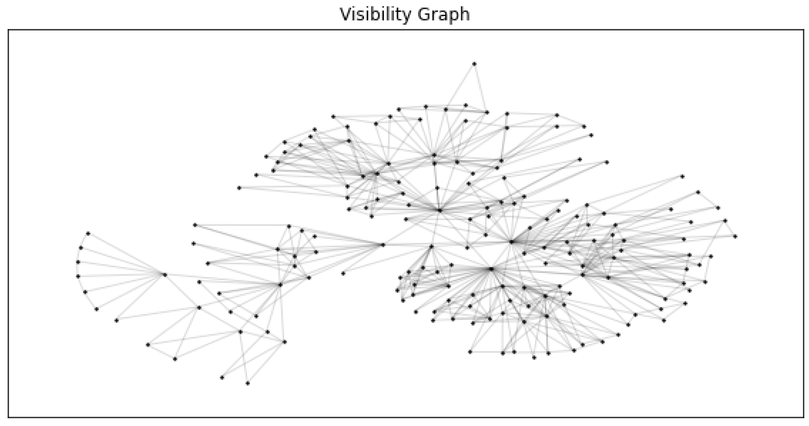
As a final result, each time series can be described as a natural visibility graph, as we describe in Figure 6.
3.5.2. Horizontal Visibility Graphs
Based on the same principles as the natural visibility graph, a new visibility graph called the horizontal visibility graph was proposed a year after its definition. Both graphs were proposed by the same team within a short period, based on the evolution of their theories [34].
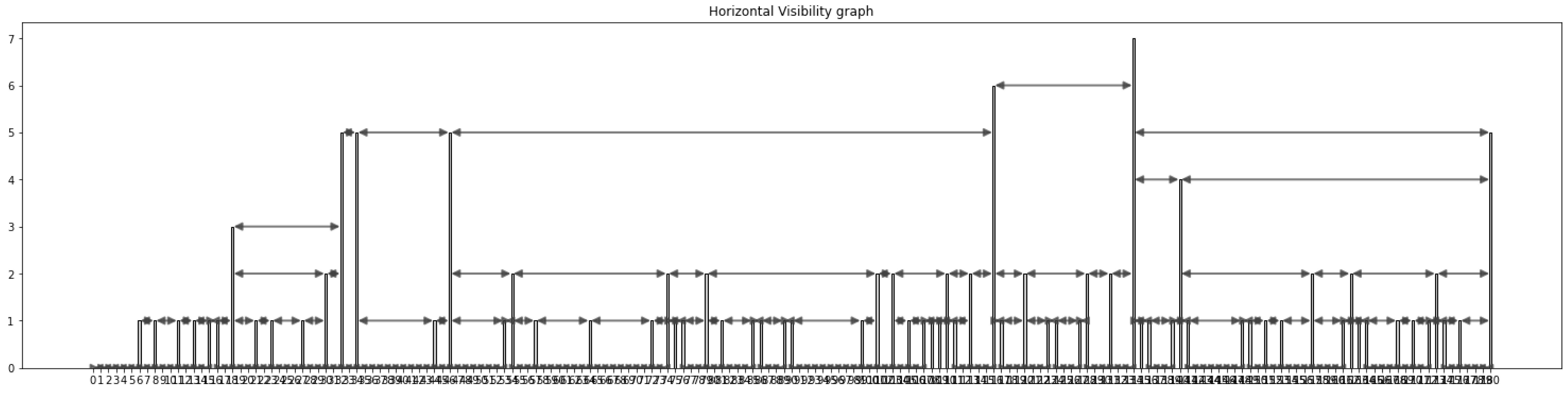
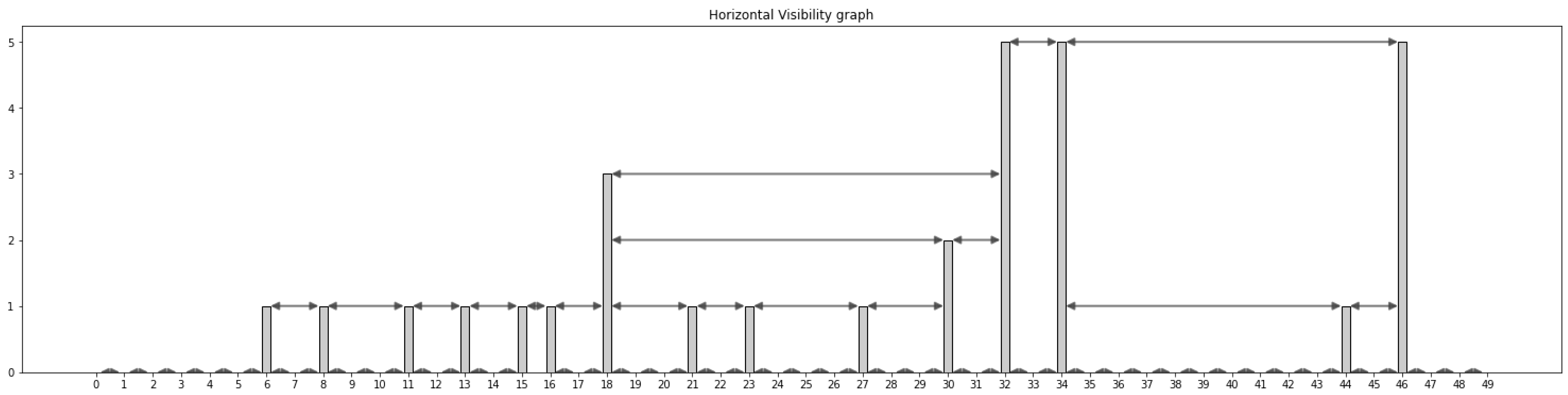
As the previous graph, this new approach is also based on the visibility of the nodes. As we can see in Figure 7 and Figure 8, the base of the creation of the graph is the same: each record of the time series is defined as a node in the visibility graph. Two nodes defined as and are connected if they have horizontal connections, that is, if we can draw a line between them without any other record height limiting their visibility.
As in the previous natural visibility graph, this new type of graph is:
- Connected, as the NVG.
- Invariant to any translation or reescalation.
- Irreversible: using the HVG, several time series can create the same HVG so that it is impossible to return from the graph to the time series. This is almost never a problem because our purpose in this operation is to catch time series structural properties. In the case where reversibility is needed, we have to use a weighted network, and to define a reversible network is feasible.
- Undirected graph. Basically, no direction is made between the two nodes. However, it is possible to create a directed graph using the temporal evolution of the time series, that is, the edge direction is the direction where the time increases in the time series.
- The natural visibility graph is a more connected graph than the HVG.
As we can see in the example below, we create the same time series as usual in the natural visibility graph, and we connect the adequate nodes. In the Figure 7, we can see the 181 records of the time series, and they are focused on the first 50 records in Figure 8. In the example, record 18 is connected to four nodes in the horizontal graph, which is much lower than the connectivity it had in the natural visibility graph.
3.6. Edge Clustering
At this moment, in a weighted network, every edge has two network graphs: the natural visibility graph and a horizontal graph. These two graphs give us the required information about the temporal behavior of the network in Figure 9.
To create an edge clustering, we take two features for every graph:
- max_degree: We define the degree of the network as the number of adjacent edges to the node. If we define a network as a set of nodes and E the set of edges connecting the nodes as , with an adjacency matrix A, we can define the max degree of the graph as
- density: We can define the density value as 0 when no edge exists on the graph. On the other hand, the value is equal to 1 if we are describing a complete graph.where n is the number of nodes and m is the number of edges in G.
For each edge, we have four features:
- Natural visibility graph max_degree,
- Natural visibility graph density,
- Horizontal visibility graph max_degree,
- Horizontal visibility graph density.
After starting from the time series created with the events over time between the nodes, transforming them into both visibility graphs and obtaining the two characteristics of each of the visibility graphs, we are ready for the groupings of these time series into similar groups, which will give us similar temporal attributes in each one.
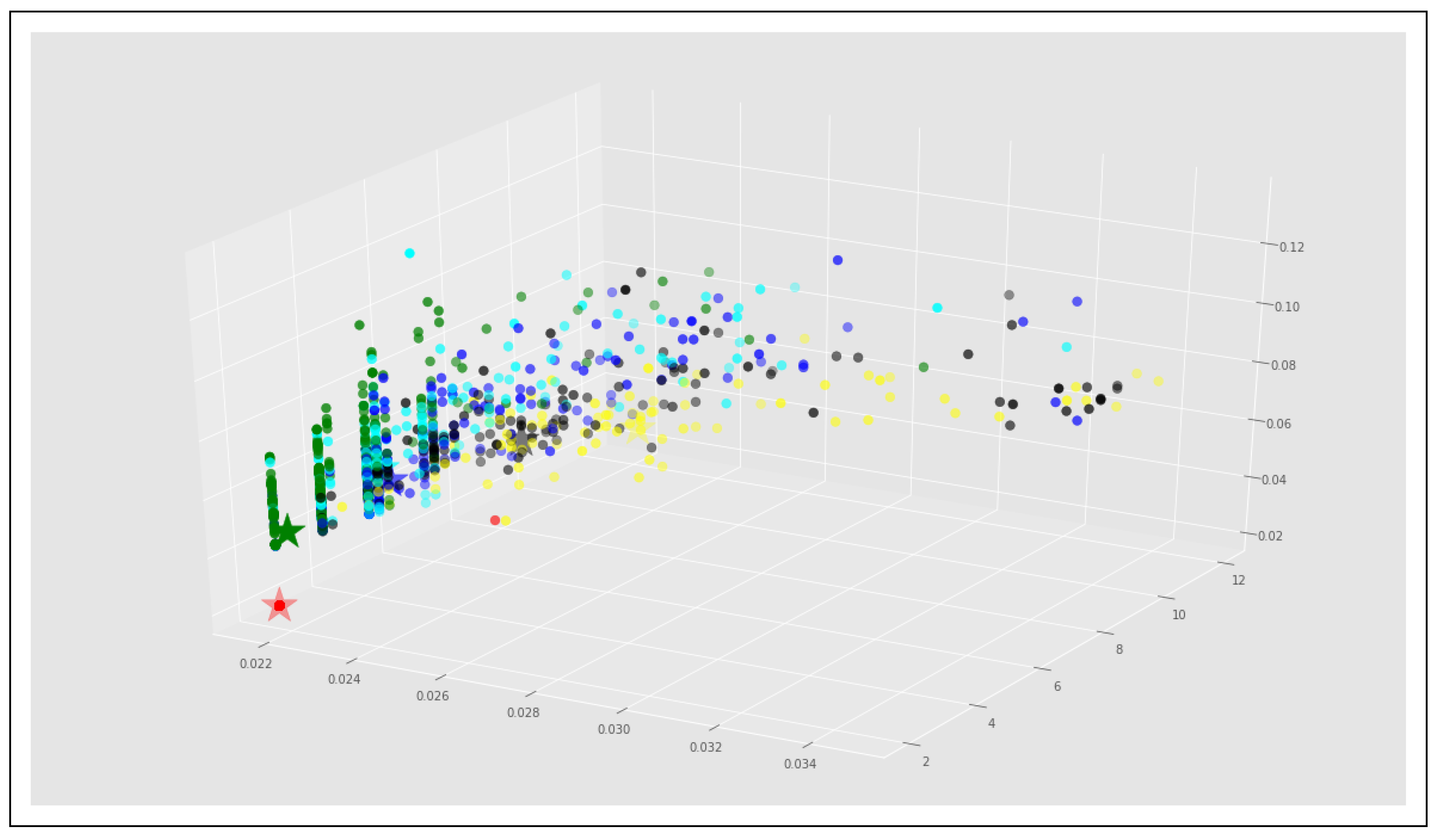
As we do not know what is the best way to cluster them, we decide to use an unsupervised machine learning algorithm to find the most convenient procedure to group them. One of the most famous algorithms for this purpose is the Kmeans, which can classify assests as we can see in Figure 10.
Kmeans is an unsupervised classification algorithm that organizes objects into k groups based on their features. Clustering is performed by minimizing the sum of distances between each object and the centroid of its group or cluster. The quadratic distance is usually used.
The algorithm consists of three steps:
- Initialization: once the number of clusters, k, has been chosen, k centroids are established in the data space; for example, by choosing them randomly.
- Assigning objects to centroids: each object in the data is assigned to its nearest centroid.
- Updating centroids: the centroid position of each group is updated by taking the position of the average of the objects belonging to that group as the new centroid.
Steps 2 and 3 are repeated until the centroids do not move, or until they move below a threshold distance in each step. The Kmeans algorithm solves an optimization problem, the function to be optimized (minimized) being the sum of the quadratic distances of each object to the centroid of its cluster. The objects are represented by d-dimensional real vectors , and the Kmeans algorithm constructs k groups where the sum of distances of the objects, within each group to its centroid. The problem can be formulated as follows:
where G is the dataset whose elements are the objects represented by vectors, where each of its elements represents a characteristic or attribute. We will have k groups or clusters with their corresponding centroid .
On each centroid update, from a mathematical point of view, we impose the necessary extremum condition on the function which, for the quadratic function before, is
and the average of the elements of each group is taken as the new centroid.
The main advantages of the Kmeans method are that it is a simple and fast method. However, it is necessary to decide on the value of k, and the final result depends on the initialization of the centroids.
With this algorithm, we can assign to each time series the best cluster, and therefore, the cluster edges in several clusters.
The more clusters, the more information that we will store about the temporal characteristics, as we will make a more accurate division of the behaviors.
3.7. Temporal Behavior Multiplex Network
Until this point, we have defined a weighted network where the edges are discrete functions based on time. These functions can be described as time series from which we have created two graphs: the natural visibility graph and the horizontal visibility graph. From these graphs, we take two features from each: max_degree and density of the networks.
With these characteristics, we have assigned finally to each time series a cluster that groups the time series having the same characteristics through an unsupervised classification system (KMeans).
In this last phase, we are going to transform our weighted graph into a multiplex network from the information that we have obtained in previous steps. As we have discussed at the beginning, graphs are the right tool to group a lot of information within them. However, at the present time, the collection of temporal features within the graphs has been rather limited.
In this case, we will deploy our weight network in N layers, where the layers in . In each of these N layers, we will include the edges that are part of the same unsupervised cluster made in previous steps.
Finally, we obtain a weighted and directed multiplex network , with n layers on a set of nodes . Each layer is defined as a weighted directed graph on the same group of nodes , and with a set of edges:
where represents the link that connects nodes x and y in , and is a function , such that for each edge , the coefficient is called weight of .
3.8. Forecasting Using Random Forest
After creating a temporal behavior multiplex network using python library networkx [35], we will use all the information inside the network to extract complex features about the temporal evolution of the node interactions.
All the characteristics obtained from the graph are complex interpretations of the interactions between the nodes in a condensed way with a small amount of information.
The most appropriate way is to find what is the best features to extract from the temporal behavior multiplex network. After several experiments, we decided to select the node degree from any node in each layer of the network. With this approach, the more layers the network has, the more features we can obtain for the realization of the following phases.
With the extracted information about the nodes, we can use any supervised machine learning algorithm to forecast any characteristic of the nodes. In our case, we have been able to detect any attackers inside the network computers analyzed.
To achieve this, after several pieces of research with different machine learning algorithms, we decided to use Random Forest. This is a fast algorithm and it is very accurate in almost all cases.
4. Results
First of all, as we have mentioned before, we create the time series with the time information about the network flows that occurred between two nodes. As we describe in the dataset section, we create a time series between the existing time slots:
- Start time: 23 April 2019 13:00:00,
- Finish time: 27 April 2019 08:00:00,
- Frequency: Hourly.
With these criteria, we obtain a time series with 91 slots where the number of bytes sent between network computers is located.
For each time series, we create a natural visibility graph and a horizontal visibility graph. From them, we take the network max degree and the density of the network. With this information, we classify the edges into six clusters where each edge could appear.
Now, we create in the network as many layers as the number of clusters that have been made in the time series, and we include each edge in the appropriate layer according to the cluster in which it has been previously assigned. Finally, every edge with a cluster attribute of value 3 will be located in layer 3 of the network.
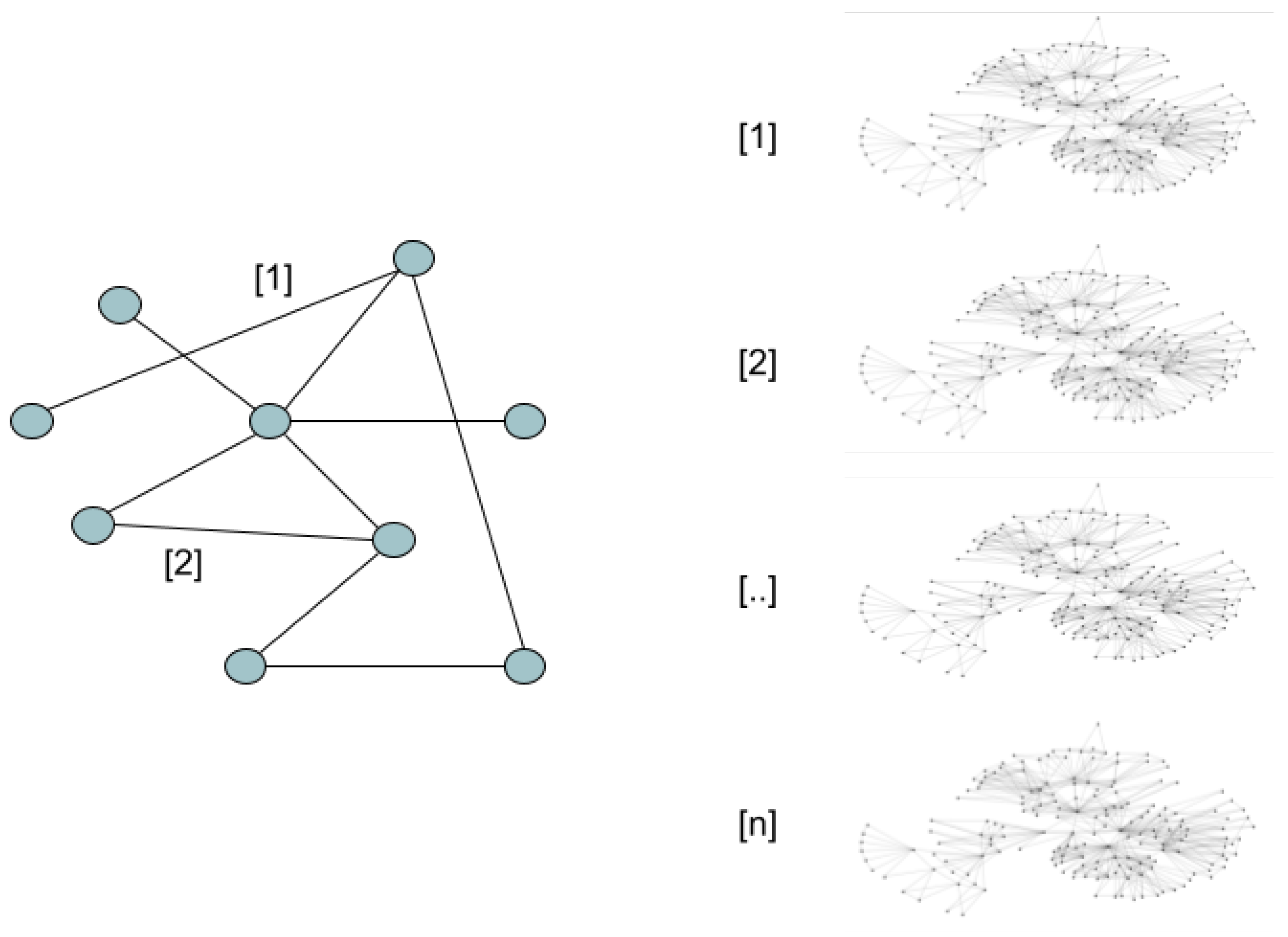
As can be seen in Figure 11, all the nodes will exist in all the layers, but the edges will only exist in the layer defined in the clustering of the time series.
This new attribute allows us to have more information in the network. With this new view, we can analyze the relationship of the nodes with the layers to detect several types of nodes. In a more complex approach, if the relationship between two nodes can be described with several time series, that is, the source and destination bytes, the multiplex network will have as many dimensions as the number of types of relationships.
Next, we show the number of nodes and edges existing in every layer (Table 2).
As we can see, the number of edges and nodes can vary, indicating different behaviors in every layer. For example, cluster 1 describes nodes with more interactions than other clusters as 2. In Table 3, Table 4, Table 5, Table 6, Table 7 and Table 8, we show the top five connected nodes in every layer, giving us complex information about the connectivity of every node in each layer.
The layers allow the nodes to be provided with additional information to the previously existing information.
Each one of the networks represents the behavior of the network of equipment analyzed differently, so it will provide additional information to the study.
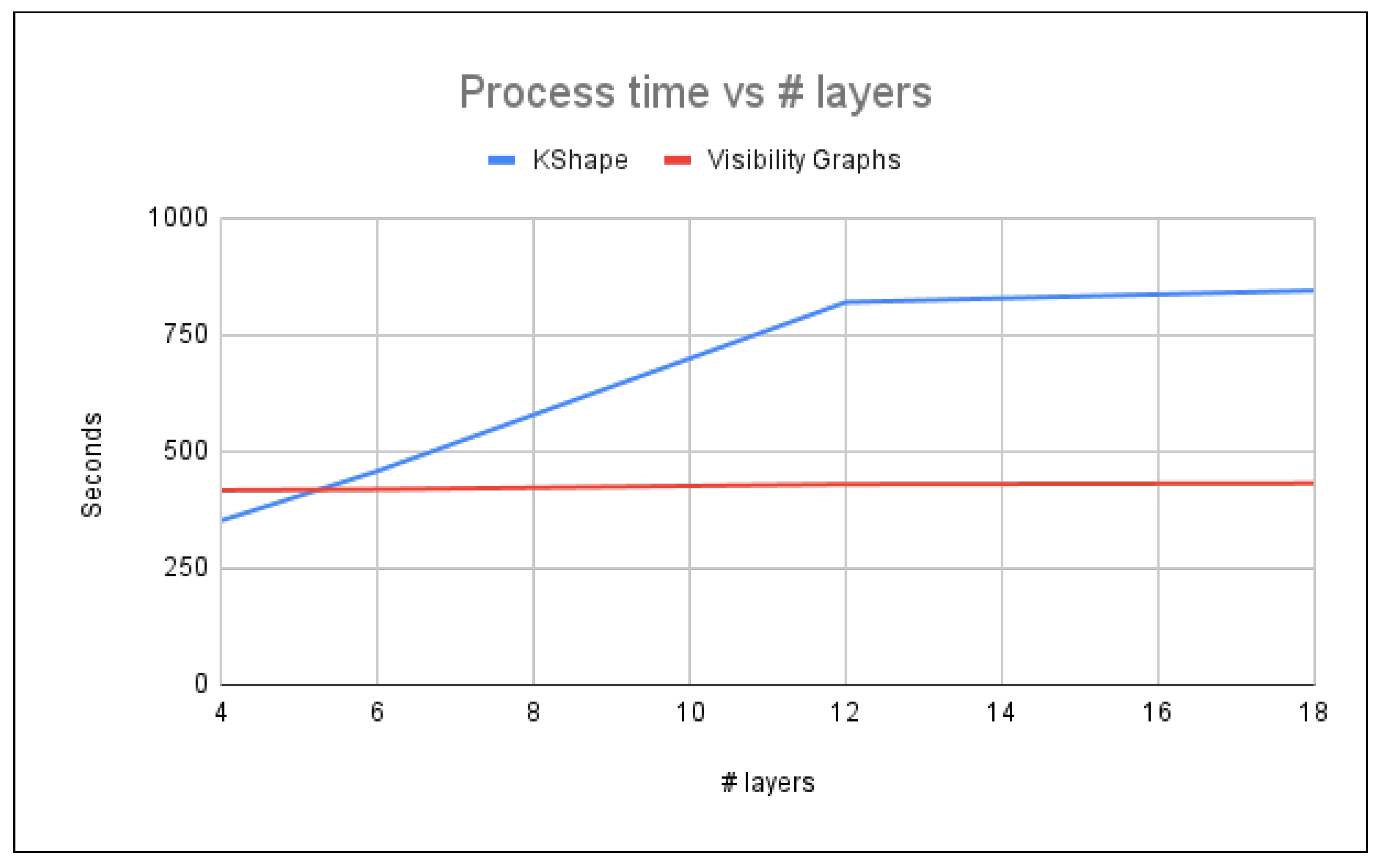
The main advantage of using visibility graphs is to reduce the process time, as we can see in Figure 12. Kshape [36] based on matrix comparison: the longer time series, the more time of computation. On the other hand, the new approach with visibility graphs maintains time regardless of what cluster number we have.
4.1. Node Features Acquisition
As we have described above, the cluster that each edge is located in is added as an attribute to the created network.
The next step is to obtain the necessary information from the multiplexed network to create a machine learning intrusion detection system. In this case, as we need to predict if an IP address (node) is an attacker, we obtain the number of neighboring nodes in each layer as a metric.
For each of the multiplex networks, we will obtain the number of edges to which the node is connected in each of the layers of the network. In our example, in the case of the network with six segments, each node will have a number of edges to which it is connected.
4.2. Attackers Detection
In this final section, based on the features generated on the temporal behavior complex network, we try to detect the attacker’s IP address with a supervised algorithm.
First of all, we present the evaluation metric that we select to validate the success of our model. It is a very relevant decision because it is important to compare it with previous research projects. Using the same evaluation metrics, we can compare our technique with other approaches made so far.
In the second section, we will describe how we develop a supervised machine learning algorithm using the node features generated above to classify every node into an attacker’s or non-attacker’s IP address.
4.2.1. Evaluation Metrics
Our proposed approach is evaluated on the dataset in terms of accuracy. This metric is widely used for model validation in a lot of research projects, so we can compare it with them to ratify our approach. The accuracy is defined as the total number of observations correctly defined concerning the total number of observations.
To understand the accuracy, another two definitions must be mentioned. In our case, a true positive is an outcome where the model correctly predicts the attacker’s IP address. Similarly, a true negative is an outcome where the model correctly predicts the non-attacker’s IP address.
4.2.2. Supervised IP Address Detection
To predict the attacker’s IP addresses, we create a supervised algorithm. As we know what are the attacker IP addresses, we take all of the variables obtained in the temporal behavior complex network and create a supervised algorithm with them.
We decide to use the Random Forest algorithm to solve this classification problem. We select it because computational cost and effectiveness are very balanced. In our case, this equilibrium gives us a simple way to compare several hyperparameters’ selections without incurring high computational costs.
In our case, this approach gives us the chance to reduce the original 72 million events to a classification algorithm with a shorter number of features for each node. This huge decrease in dimension is thanks to the temporal behavior complex network.
As with every classification problem, we follow the standard phases to fit the model with the actual dataset.
- Cross-validation: to avoid overfitting problems. It is very important to use cross-validation to obtain stable accuracy in the model. CV consists of randomly dividing the data into N groups; all groups except one trains the model, and the last tests it. This process is repeated N times, and their average accuracy is selected as the final accuracy. In our case, we use the class StratifiedKFold from the python sklearn package. We use this class instead of KFold because it preserves the percentage of samples for each class. Our case is a high imbalance dataset, and so it is very relevant to maintain the class balance. By default, the number of folds is set to 5, but we decide to increase them to 10 to obtain a more accurate prediction.
- Train-test: We divide the dataset into two different parts. The first one (train) is used to fit the model, and the other (test) is used to validate the fitted model. The StratifiedKFold class gives us, in our case, 10 train datasets and 10 test datasets to create a model for each pair.
- The Random Forest algorithm has several hyperparameters to select. We use a grid search technique to select the best result for our project. One of the most relevant parameters to tune is the number of estimators. In our case, after comparing between several values, we decided to use 100 as the best number of estimators.
Once this is achieved, we use a Random Forest model with 100 estimators to make a predictive model. As we have 10 different models, we use their mean accuracy to validate the mean accuracy of the model. All of these steps are described in Algorithm 1.
| Algorithm 1 Cross Validation. |
| for train_index, test_index in skf.split(X, y) do end for |
This model predicts the detection of IP attacker addresses with a multiplex network of four layers with an accuracy of 99.8%.
4.2.3. Comparison with the Previous Approach
5. Discussion
5.1. Conclusions
In this work, we present a new approach for the deployment of NIDS in large corporations based on the analysis of the behavior of the network IP address instead of the traditional detection techniques based on the analysis of every network event packet in the network. This new approach gives us two advantages compared to the traditional NIDS:
- Reducing the number of alerts generated by the NIDS to be analyzed by the SOC analyst: The accuracies of the actual NIDS and machine learning approaches are very high; however, analyzing every network packet gives us a lot of alerts due to the large number of events crossing the networks, and in most cases, these alerts with a correct context about the IP address and the behavior of the relation between them makes it easier for the SOC analyst to discard them. However, this action redirects the focus on the correct alert where the behavior gives us the reason to analyze this relationship in depth.
- Reducing the computational requirements, decreasing the analysis to time slots instead of every network event. For example, if a behavior analysis is made every 5 min, we can change the depth of analysis of every packet in this slot of time to the behavior analysis for the relations of the existing IP address. This reduces the potential alert from thousands to hundreds.
Furthermore, the combination of the time series and the complex networks gives us a new technique to for analyzing the behavior of every relation between two IP addresses and detecting the malicious behavior that the SOC analyst must analyze.
5.2. Next Steps
In this paper, we describe a new approach for aggregating events to obtain a temporal multiplex network, and we use a known dataset to validate the efficiency of the new approach in a real challenge.
Based on this paper, there are several new studies to perform:
- Validating this type of data in large corporate environments.
- Changing unsupervised time series clustering techniques to supervised techniques. This approach gives us a better understanding of the description of every cluster.
- Using other time series techniques to obtain more information about the behavior of the relationship between the nodes.
- Using this new dataset in cybersecurity with the same approach to confirm the same accuracy obtained in this paper.
- Using this approach to solve others’ real-world problems.
- Predicting with complex network capabilities rather than with Random Forest.
Author Contributions
Conceptualization, S.I.P. and R.C.; methodology, S.I.P.; formal analysis, S.I.P. and R.C.; investigation, S.I.P.; resources, S.I.P.; data curation, S.I.P.; writing—original draft preparation, S.I.P.; writing—review and editing, R.C.; supervision, R.C. All authors have read and agreed to the published version of the manuscript.
Funding
This research received no external funding.
Data Availability Statement
The data used to support the findings of this study are available from the corresponding author upon request.
Conflicts of Interest
The authors declare no conflict of interest.
Abbreviations
The following abbreviations are used in this manuscript:
| NIDS | Network Intrusion Detection System |
| UEBA | User Entity Behavior Analytics |
| MTTD | Mean Time To Detection |
| SIEM | Security Information and Event Management |
| SOC | Security Operation Control |
References
- Dorogovtsev, S. Complex Networks; Oxford University Press: Oxford, UK, 2010. [Google Scholar]
- Strogatz, S.H. Exploring complex networks. Nature 2001, 410, 268–276. [Google Scholar] [CrossRef] [PubMed] [Green Version]
- Boccaletti, S.; Bianconi, G.; Criado, R.; DelGenio, C.I.; Gómez-Gardeñes, J.; Romance, M.; Sendixnxa-Nadal, I.; Wang, Z.; Zanin, M. The structure and dynamics of multilayer networks. Phys. Rep. 2014, 544, 1–122. [Google Scholar] [CrossRef] [Green Version]
- Da Fontoura Costa, L.; Oliveira, O.N.; Travieso, G.; Rodrigues, F.A.; Villas Boas, P.R.; Antiqueira, L.; Viana, M.P.; Correa Rocha, L.E. Analyzing and modeling real-world phenomena with complex networks: A survey of applications. Adv. Phys. 2011, 60, 329–412. [Google Scholar] [CrossRef] [Green Version]
- Kivela, M.; Arenas, A.; Barthelemy, M.; Gleeson, J.P.; Moreno, Y.; Porter, M.A. Multilayer Networks. J. Complex Netw. 2014, 2, 203–227. [Google Scholar] [CrossRef] [Green Version]
- Chapela, V.; Criado, R.; Moral, S.; Romance, M. Intentional Risk Management through Complex Networks Analysis; Springer International Publishing: Berlin/Heidelberg, Germany; New York, NY, USA; Dordrecht, The Netherlands; London, UK, 2015. [Google Scholar]
- Criado, R.; Moral, S.; Pérez, A.; Romance, M. On the edges’s PageRank and linegraphs. Chaos 2018, 28, 075503. [Google Scholar] [CrossRef] [PubMed]
- Estrada, E. Networks Science; Springer: New York, NY, USA, 2010. [Google Scholar]
- Latora, V.; Nicosia, V.; Russo, G. Complex Networks: Principles, Methods and Applications; Cambridge University Press: Cambridge, UK, 2017. [Google Scholar]
- Moral, S.; Chapela, V.; Criado, R.; Pérez, A.; Romance, M. Efficient algorithms for estimating loss of information in a complex network: Applications to intentional risk analysis. Netw. Heterog. Media 2015, 10, 195–208. [Google Scholar]
- Newman, M. Networks: An Introduction; Oxford University Press: Oxford, UK, 2010. [Google Scholar]
- Zanin, M.; Romance, M.; Moral, S.; Criado, R. Credit Card Fraud Detection through Parenclitic Network Analysis. Complexity 2018, 2018, 5764370. [Google Scholar] [CrossRef]
- Zanin, M.; Papo, D.; Romance, M.; Criado, R.; Moral, S. The topology of card transaction money flows. Phys. A 2016, 462, 134–140. [Google Scholar] [CrossRef] [Green Version]
- Partida, A.; Criado, R.; Romance, M. Identity and Access Management Resilience against Intentional Risk for Blockchain-Based IOT Platforms. Electronics 2021, 10, 378. [Google Scholar] [CrossRef]
- Partida, A.; Criado, R.; Romance, M. Visibility Graph Analysis of IOTA and IoTeX Price Series: An Intentional Risk-Based Strategy to Use 5G for IoT. Electronics 2021, 10, 2282. [Google Scholar] [CrossRef]
- Criado-Alonso, A.; Battaner-Moro, E.; Aleja, D.; Romance, M.; Criado, R. Using complex networks to identify patterns in specialty mathematical language: A new approach. Soc. Netw. Anal. Min. 2020, 10, 69. [Google Scholar] [CrossRef]
- Iglesias, S.; Moral-Rubio, S.; Criado, R. A new approach to combine multiplex networks and time series attributes: Building intrusion detection systems (IDS) in cybersecurity. Chaos Solitons Fractals 2021, 150, 111143. [Google Scholar] [CrossRef]
- Perez, S.I.; Moral-Rubio, S.; Criado, R. Combining multiplex networks and time series: A new way to optimize real estate forecasting in New York using cab rides. Phys. A Stat. Mech. Its Appl. 2022, 609, 128306. [Google Scholar] [CrossRef]
- Aburomman, A.; Reaz, M.B.I. Review of ids develepment methods in machine learning. Int. J. Electr. Comput. Eng. 2016, 6, 2432. [Google Scholar] [CrossRef] [Green Version]
- Tsai, C.-F.; Hsu, Y.-F.; Lin, C.-Y.; Lin, W.-Y. Intrusion detection by machine learning: A review. Expert Syst. Appl. 2009, 36, 11994–12000. [Google Scholar] [CrossRef]
- Sethi, K.; Sai Rupesh, E.; Kumar, R.; Bera, P.; Venu Madhav, Y. A context-aware robust intrusion detection system: A reinforcement learning-based approach. Int. J. Inf. Secur. 2020, 19, 657–678. [Google Scholar] [CrossRef]
- Khan, M.A.; Karim, M.R.; Kim, Y. A Scalable and Hybrid Intrusion Detection System Based on the Convolutional-LSTM Network. Symmetry 2019, 11, 583. [Google Scholar] [CrossRef] [Green Version]
- Muna, A.H.; Moustafa, N.; Sitnikova, E. Identification of malicious activities in industrial internet of things based on deep learning models. J. Inf. Secur. Appl. 2018, 41, 1–11. [Google Scholar] [CrossRef]
- Tama, B.A.; Rhee, K.H. Attack Classification Analysis of IoT Network via Deep Learning Approach. Res. Briefs Inf. Commun. Technol. Evol. (ReBICTE) 2017, 3, 1–9. [Google Scholar] [CrossRef]
- Viet, H.N.; Van, Q.N.; Trang, L.L.T.; Nathan, S. Using Deep Learning Model for Network Scanning Detection. In Proceedings of the 4th International Conference on Frontiers of Educational Technologies, Moscow, Russia, 25–27 June 2018. [Google Scholar] [CrossRef] [Green Version]
- Van, N.T.; Thinh, T.N.; Sach, L.T. A Combination of Temporal Sequence Learning and Data Description for Anomaly-based NIDS. arXiv 2019, arXiv:1906.05277. [Google Scholar]
- Anton, S.D.; Ahrens, L.; Fraunholz, D.; Schotten, H. Time is of the essence: Machine learning-based intrusion detection in industrial time series data. In Proceedings of the 2018 IEEE International Conference on Data Mining Workshops (ICDMW), Singapore, 17–20 November 2018; pp. 1–6. [Google Scholar] [CrossRef]
- Wang, F.; Yang, S.; Wang, C.; Li, Q. A Novel Intrusion Detection System for Malware Based on Time-Series Meta-learning. In Proceedings of the International Conference on Machine Learning for Cyber Security, Guangzhou, China, 8–10 October 2020; Springer: Cham, Switzerland, 2020; pp. 50–64. [Google Scholar]
- Staniford-Chen, S.; Cheung, S.; Crawford, R.; Dilger, M.; Frank, J.; Hoagland, J.; Zerkle, D. A graph based intrusion detection system for large networks. In Proceedings of the 19th National Information Systems Security Conference, Baltimore, MD, USA, 22–25 October 1996. [Google Scholar]
- Akoglu, L.; Tong, H.; Koutra, D. Graph-based anomaly detection and description: A survey. arXiv 2014, arXiv:1404.4679. [Google Scholar] [CrossRef] [Green Version]
- Shang, K.K.; Small, M.; Xu, X.K.; Yan, W.S. The role of direct links for link prediction in evolving networks. EPL (Europhys. Lett.) 2017, 117, 28002. [Google Scholar] [CrossRef]
- Ashraf, J.; Keshk, M.; Moustafa, N.; Abdel-Basset, M.; Khurshid, H.; Bakhshi, A.D.; Mostafa, R.R. IoTBoT-IDS: A Novel Statistical Learning-enabled Botnet Detection Framework for Protecting Networks of Smart Cities. Sustain. Cities Soc. 2021, 72, 103041. [Google Scholar] [CrossRef]
- Lacasa, L.; Luque, B.; Ballesteros, F.; Luque, J.; Nuno, J.C. From time series to complex networks: The visibility graph. Proc. Natl. Acad. Sci. USA 2008, 105, 4972–4975. [Google Scholar] [CrossRef] [PubMed] [Green Version]
- Luque, B.; Lacasa, L.; Ballesteros, F.; Luque, J. Horizontal visibility graphs: Exact results for random time series. Phys. Rev. Stat. Nonlinear Soft Matter Phys. 2009, 80, 046103. [Google Scholar] [CrossRef] [Green Version]
- Hagberg, A.; Swart, P.; Chult, D.S. Exploring network structure, dynamics, and function using NetworkX. In Proceedings of the 7th Python in Science Conference (SciPy2008), Pasadena, CA, USA, 19–24 August 2008; Varoquaux, G., Vaught, T., Millman, J., Eds.; Los Alamos National Lab: Los Alamos, NM, USA, 2008; pp. 11–15. [Google Scholar]
- Paparrizos, J.; Gravano, L. k-Shape: Efficient and Accurate Clustering of Time Series. ACM SIGMOD Rec. 2016, 45, 69–76. [Google Scholar] [CrossRef]
- Koroniotis, N.; Moustafa, N.; Sitnikova, E.; Turnbull, B. Towards the development of realistic botnet dataset in the internet of things for network forensic analytics: Bot-iot dataset. Future Gener. Comput. Syst. 2019, 100, 779–796. [Google Scholar] [CrossRef] [Green Version]
- Shafiq, M.; Tian, Z.; Bashir, A.K.; Du, X.; Guizani, M. CorrAUC: A malicious bot-iot traffic detection method in iot network using machine learning techniques. IEEE Internet Things J. 2020, 8, 3242–3254. [Google Scholar] [CrossRef]
- Khraisat, A.; Gondal, I.; Vamplew, P.; Kamruzzaman, J.; Alazab, A. A novel ensemble of hybrid intrusion detection system for detecting internet of things attacks. Electronics 2019, 8, 1210. [Google Scholar] [CrossRef] [Green Version]
- Churcher, A.; Ullah, R.; Ahmad, J.; Rehman, S.U.; Masood, F.; Gogate, M.; Alqahtani, F.; Nour, B.; Buchanan, W.J. An experimental analysis of attack classification using machine learning in iot networks. Sensors 2021, 21, 446. [Google Scholar] [CrossRef]
- Zeeshan, M.; Riaz, Q.; Bilal, M.A.; Shahzad, M.K.; Jabeen, H.; Haider, S.A.; Rahim, A. Protocol Based Deep Intrusion Detection for DoS and DDoS attacks using UNSW-NB15 and Bot-IoT data-sets. IEEE Access 2021, 10, 2269–2283. [Google Scholar] [CrossRef]
Figure 1.
IoT endpoint market evolution, 2018–2020.

Figure 2.
Mean Time To Detect Average by year.

Figure 3.
IDS architecture.

Figure 4.
Research workflow.

Figure 5.
Time series to visibility graph conversion.

Figure 6.
Time series to visibility graph conversion.

Figure 7.
Timeseries to visibility graph conversion.

Figure 8.
Timeseries to visibility graph conversion. First 50 days.

Figure 9.
Visibilitygraph as edge.

Figure 10.
Classification in 6 clusters.

Figure 11.
Example of multiplex network with 6 layers.

Figure 12.
Process time comparison between Kshape and visibility graphs.


Table 1.
List of features located in the proposed dataset.
| Title 1 | Title 2 |
|---|---|
| ts | src_ip |
| src_port | dst_ip |
| dst_port | proto |
| service | duration |
| src_bytes | dst_bytes |
| conn_state | missed_bytes |
| src_pkts | src_ip_bytes |
| dst_pkts | dst_ip_bytes |
| dns_query | ns_qclass |
| dns_qtype | dns_rcode |
| dns_AA | dns_RD |
| dns_RA | dns_rejected |
| ssl_version | ssl_cipher |
| ssl_resumed | ssl_established |
| ssl_subject | ssl_issuer |
| http_trans_depth | http_method |
| http_uri | http_version |
| http_request_body_len | |
| http_response_body_len | http_status_code |
| http_user_agent | http_orig_mime_types |
| http_resp_mime_types | weird_name |
| weird_addl | weird_notice |
| label | type |
Table 2.
Distribution of nodes and edges in layers.
| Cluster | Number of Edges | Number of Nodes |
|---|---|---|
| 0 | 25,093 | 24,336 |
| 1 | 4207 | 3952 |
| 2 | 166 | 166 |
| 3 | 392 | 377 |
| 4 | 409 | 411 |
| 5 | 102 | 106 |
Table 3.
Top 5 nodes in the layer from Cluster 0 edges.
| Node | Connected Edges |
|---|---|
| 192.168.1.194 | 9257 |
| 192.168.1.190 | 5728 |
| 192.168.1.152 | 5284 |
| 192.168.1.184 | 3358 |
| 192.168.1.2 | 256 |
Table 4.
Top 5 nodes in the layer from Cluster 1 edges.
| Node | Connected Edges |
|---|---|
| 192.168.1.190 | 3503 |
| 192.168.1.195 | 138 |
| 192.168.1.180 | 123 |
| 192.168.1.30 | 101 |
| 192.168.1.31 | 89 |
Table 5.
Top 5 nodes in the layer from Cluster 2 edges.
| Node | Connected Edges |
|---|---|
| 192.168.1.190 | 113 |
| 192.168.1.195 | 20 |
| 192.168.1.180 | 18 |
| 192.168.1.193 | 9 |
| 192.168.1.30 | 4 |
Table 6.
Top 5 nodes in the layer from Cluster 3 edges.
| Node | Connected Edges |
|---|---|
| 192.168.1.190 | 296 |
| 192.168.1.195 | 25 |
| 192.168.1.180 | 24 |
| 192.168.1.30 | 14 |
| 192.168.1.31 | 13 |
Table 7.
Top 5 nodes in the layer from Cluster 4 edges.
| Node | Connected Edges |
|---|---|
| 192.168.1.190 | 354 |
| 192.168.1.195 | 18 |
| 192.168.1.180 | 14 |
| 192.168.1.193 | 8 |
| 192.168.1.30 | 5 |
Table 8.
Top 5 nodes in the layer from Cluster 5 edges.
| Node | Connected Edges |
|---|---|
| 192.168.1.190 | 71 |
| 192.168.1.195 | 21 |
| 192.168.1.31 | 3 |
| 192.168.1.180 | 3 |
| 192.168.1.1 | 3 |
Disclaimer/Publisher’s Note: The statements, opinions and data contained in all publications are solely those of the individual author(s) and contributor(s) and not of MDPI and/or the editor(s). MDPI and/or the editor(s) disclaim responsibility for any injury to people or property resulting from any ideas, methods, instructions or products referred to in the content. |
© 2022 by the authors. Licensee MDPI, Basel, Switzerland. This article is an open access article distributed under the terms and conditions of the Creative Commons Attribution (CC BY) license (https://creativecommons.org/licenses/by/4.0/).
Share and Cite
MDPI and ACS Style
Iglesias Perez, S.; Criado, R. Increasing the Effectiveness of Network Intrusion Detection Systems (NIDSs) by Using Multiplex Networks and Visibility Graphs. Mathematics 2023, 11, 107. https://doi.org/10.3390/math11010107
AMA Style
Iglesias Perez S, Criado R. Increasing the Effectiveness of Network Intrusion Detection Systems (NIDSs) by Using Multiplex Networks and Visibility Graphs. Mathematics. 2023; 11(1):107. https://doi.org/10.3390/math11010107
Chicago/Turabian StyleIglesias Perez, Sergio, and Regino Criado. 2023. "Increasing the Effectiveness of Network Intrusion Detection Systems (NIDSs) by Using Multiplex Networks and Visibility Graphs" Mathematics 11, no. 1: 107. https://doi.org/10.3390/math11010107
Note that from the first issue of 2016, this journal uses article numbers instead of page numbers. See further details here.