Multi-Step-Ahead Wind Speed Forecast Method Based on Outlier Correction, Optimized Decomposition, and DLinear Model

Abstract

Precise and dependable wind speed forecasting (WSF) enables operators of wind turbines to make informed decisions and maximize the use of available wind energy. This study proposes a hybrid WSF model based on outlier correction, heuristic algorithms, signal decomposition methods, and DLinear. Specifically, the hybrid model (HI-IVMD-DLinear) comprises the Hampel identifier (HI), the improved variational mode decomposition (IVMD) optimized by grey wolf optimization (GWO), and DLinear. Firstly, outliers in the wind speed sequence are detected and replaced with the HI to mitigate their impact on prediction accuracy. Next, the HI-processed sequence is decomposed into multiple sub-sequences with the IVMD to mitigate the non-stationarity and fluctuations. Finally, each sub-sequence is predicted by the novel DLinear algorithm individually. The predictions are reconstructed to obtain the final wind speed forecast. The HI-IVMD-DLinear is utilized to predict the real historical wind speed sequences from three regions so as to assess its performance. The experimental results reveal the following findings: (a) HI could enhance prediction accuracy and mitigate the adverse effects of outliers; (b) IVMD demonstrates superior decomposition performance; (c) DLinear has great prediction performance and is suited to WSF; and (d) overall, the HI-IVMD-DLinear exhibits superior precision and stability in one-to-four-step-ahead forecasting, highlighting its vast potential for application.

1. Introduction

The finite and non-renewable nature of fossil fuels has rendered the development and utilization of renewable energy an indispensable choice [1]. A report published in 2021 stated that the cumulative installed capacity of wind farms globally skyrocketed to 744 GW [2]. However, the inherent volatility and instability of wind energy led to frequent fluctuations in wind power, thereby causing continuous oscillations in grid voltage and frequency, which severely impairs power quality. Precise and dependable WSF are important for all aspects of wind power systems, including electricity market operation, energy storage system management, network planning, etc.

Recently, numerous forecasting methods have been developed to achieve WSF based on different time scales. These methods primarily include physical methods, statistical methods, machine learning methods, and neural network models. Physical methods rely on physical factors such as altitude and atmospheric pressure to construct models to predict the changes in wind speed. However, most physical factors are difficult to obtain in the vast majority of situations. Additionally, the construction and the calculation of physical models are complex, which makes it difficult to obtain accurate WSF in a short period [3,4,5]. Luckily, statistical methods such as the autoregressive (AR) [6] and autoregressive integrated moving average (ARIMA) methods [7,8] operate at a fast pace. These models were constructed mainly based on historical wind speed operational data. However, statistical methods can only deal with linear data, but not with nonlinear wind speed series. In addition, machine learning methods such as XGBoost [9], support vector regression (SVR) [10,11], and least squares support vector machine (LSSVM) [12] can identify more complex nonlinear relationships in sequences with good generalization abilities. Usually, the predictive performance of machine learning models on large datasets is limited. Compared with conventional machine learning models, neural networks are favorite due to their unique fully connected structure, which promises better prediction accuracy on large datasets. However, neural networks have not fully considered the temporal properties of wind speed sequences. There exists a loss of temporal information in wind speed sequences since neural networks treat time series as unordered and assign equal weight to all time points [13,14,15].

To address this issue, the recurrent neural network (RNN) was proposed. The self-connection among hidden layers in the RNN enables the retention of prior states, which are then incorporated into the current step. This mechanism facilitates the consideration of temporal information during the processing of sequential data [16]. It has two main variations: long short-term memory (LSTM) [17,18,19] and gated recurrent unit (GRU) [20,21,22]. LSTM resolves the problem of gradient vanishing and exploding encountered in RNN by introducing gate mechanisms and a special memory cell structure. Satyam et al. designed a wind speed prediction method with LSTM [17]. GRU is an improvement of LSTM based on a simpler memory cell structure with only two gates (reset gate and update gate) than LSTM. GRU outperforms LSTM in terms of computational efficiency and storage space [20,21,22]. Syu et al. introduced a WSF model based on GRU to provide more precise WSF than RNN and LSTM [23]. Although LSTM and GRU have shown good performance, they usually only model short-term dependencies, while the transformer can handle longer sequences of dependencies since it does not have a recurrent structure and can simultaneously view the entire sequence at all time steps. Furthermore, the self-attention mechanism of the transformer can capture local and global dependencies in a sequence, which can better handle key information in the sequence [24,25,26]. Wu et al. devised a multi-step WSF model based on the transformer, treating the problem as a sequence-to-sequence mapping. The transformer-based model has better prediction performance than the GRU [26]. However, Zeng et al. indicated that the comparatively elevated long-term forecasting accuracy of the transformer does not substantially correlate with its capability to extract temporal dependencies, and proposed a structurally simple DLinear model with better performance than the complex transformer model in most cases [27]. The effectiveness of WSF based on the transformer model should be reevaluated. Currently, the transformer model is widely employed in the field of WSF, yet its effectiveness in this domain is questionable. Its intricate structure does not improve the forecasting accuracy. To validate this proposition about the transformer, this study utilizes the DLinear as the foundational model for prediction, considering the transformer model as a comparable model. Furthermore, another reason to adopte the DLinear mode is its remarkably simple structure, which has exceptional forecasting accuracy.

Numerous studies have shown that, because of the non-stationarity and strong volatility of wind speed sequences, models with decomposition methods perform better in predicting wind speed than those without decomposition [25,28,29,30]. Decomposition-based models usually decompose the wind speed sequence into multiple sub-sequences, then forecast each sub-sequence, and then the ultimate prediction can be obtained by aggregating the results. Currently, the popular decomposition methods include wavelet transform (WT) [31,32], empirical mode decomposition (EMD) [33,34], and ensemble empirical mode decomposition (EEMD) [35,36]. Zhang et al. decomposed the initial wind speed sequence into finite sub-sequences by the complete ensemble empirical mode decomposition with adaptive noise (CEEMDAN) algorithm [37]. Subsequently, prediction models were applied to each sub-sequence to make individual forecasts. On the other hand, Pan et al. introduced the VMD method to decompose wind speed signals and exploit their latent information for more accurate forecasting results [38]. Li et al. decomposed ship-radiated noise signals, extracting feature information of different frequencies and amplitudes with successive variational mode decomposition (SVMD) [39]. Furthermore, VMD displays superior performance in decomposing non-stationary signals when compared to EMD and its improved methods [40]. Nevertheless, VMD lacks adaptability because critical parameters, e.g., the number of decomposition modes and regularization, require manual adjustment. The choice of these two parameters can impact the decomposition results and performance significantly. Moreover, the grey wolf optimization (GWO) algorithm exhibits superior optimization capabilities compared to renowned algorithms including particle swarm optimization, gravitational search algorithm, and evolution strategy [41]. Consequently, in this paper, the hyperparameters of VMD will be optimized by the GWO algorithm, thereby addressing the challenge of selecting the appropriate hyperparameters of VMD.

Additionally, there are few researches focusing on detecting and correcting outliers in the original wind speed sequence. It is reported that the predictive accuracy could be enhanced by rectifying outliers within the original sequence [42]. To detect and rectify outliers in the original wind speed sequence, the HI algorithm [43] is introduced to enhance the final accuracy of wind speed prediction.

In recent years, various metrics such as entropy [44] and correlation dimension [45] have been extensively employed in signal analysis across various research domains. Li et al. introduced an innovative technique known as simplified coded dispersion entropy (SCDE) to identify nonlinear dynamic transitions in signals [44]. A novel approach called FuzzDEα was developed to detect dynamic changes in time series data for signal analysis and fault diagnosis in bearings [46]. To assess the level of optimization of the hyperparameters of VMD by GWO, the envelope entropy (EE) [47] as the fitness function for GWO was employed. The magnitude of the EE serves as a criterion to evaluate the quality of the hyperparameters obtained by GWO. The magnitude of SampEn reflects the complexity level of a time series. If the series exhibits higher complexity, the corresponding SampEn value will be larger; conversely, a lower complexity will result in a smaller SampEn value [48]. Therefore, in this study, the SampEn will be utilized to assess the effectiveness of the HI.

Synthetically speaking, to achieve high accuracy and stability in WSF, a hybrid model is proposed based on outlier correction, heuristic algorithms, signal decomposition methods, and DLinear. The model begins by employing the HI to detect and rectify outliers in the original wind speed sequence. Subsequently, the GWO algorithm is utilized to optimize the hyperparameters of the VMD. Then, employing the VMD algorithm based on the optimal hyperparameters, the sequence processed by HI is decomposed into several sub-sequences. Lastly, each sub-sequence is forecasted by the DLinear algorithm individually. The final wind speed forecast is obtained by reconstructing the predictions. The primary contributions of this study are as follows:

(1)

To detect and rectify outliers in the wind speed sequence, an outlier detection technique based on the Hampel identifier (HI) is utilized to enhance the accuracy of WSF.

(2)

To optimize the hyperparameters of VMD, the variational mode decomposition is improved by the grey wolf optimization (GWO). The decomposition of the complex non-stationary windspeed sequence with the improved VMD (IVMD) algorithm can reduce the non-stationarity and the complexity of the sequence, thus improving the prediction stability and accuracy.

(3)

DLinear is introduced as a fundamental prediction model including only one decomposition scheme and two linear networks. Its performance is significantly superior to both LSTM and the currently popular transformer models.

(4)

The proposed method combining HI and IVMD with DLinear is utilized for the multi-step WSF of three real windspeed sequences. The performance of the HI-IVMD-DLinear is validated with comparative experiments from various aspects.

The rest of the paper is organized as follows: In Section 2, HI, GWO, VMD, DLinear, and the proposed method are described in detail. Section 3 elucidates the experimental configuration and elaborates, based on multiple evaluation criteria, on the performance of the proposed model. Section 4 provides a detailed discussion on the computational efficiency and the complexity of the HI-IVMD-DLinear. Finally, a concise conclusion is stated in Section 5.

2. Materials and Methods

2.1. Hampel Identifier

Hampel identifier (HI) is a robust algorithm to detect and replace outliers in datasets [43]. This method identifies any value that falls outside of a certain distance window from the median as an outlier and replaces it with the median value within that window. For dataset $D=\left[y_1,y_2,\dots ,y_n\right]$, let the window size be $w=2k+1$. Typically, window sizes of 5 or 7 are commonly used. The evaluation parameter $\alpha$ is set as 0.6745. By utilizing the median absolute deviation (MAD) and $\alpha$, the standard deviation ${\sigma }_i$ can be determined [49].

The HI method is composed of the following steps:

(1)

Computing median, MAD, and standard deviation: For each data point, the median and the MAD of the neighboring points within the window size are calculated, and then the standard deviation based on the median and MAD can be computed as [42]:

$$m_i=\mathrm{median}\left(y_{i-n},y_{i-n+1},\dots ,y_i,\dots ,y_{i+n-1},y_{i+n}\right)$$

(1)

$${\mathrm{MAD}}_i=\mathrm{median}\left(\left|y_{i-n}-m_i\right|,\left|y_{i-n+1}-m_i\right|,\dots ,\left|y_i-m_i\right|,\dots ,\left|y_{i+n-1}-m_i\right|,\left|y_{i+n}-m_i\right|\right)$$

(2)

$${\sigma }_i={\mathrm{MAD}}_i/\alpha$$

(3)

(2)

Detecting outlier points: A sample point is considered as an outlier if its value satisfies [50]:

$$\left|y_i-m_i\right|>3{\sigma }_i$$

(4)

(3)

Substituting outlier points: For the identified outlier points, the median of the window is used for substitution.

(4)

Performing steps (1)–(3) for each sample point.

The HI method has more advantages over other similar methods in terms of robustness to outliers. Additionally, the HI method is highly efficient in computation, making it suitable for large-scale datasets. Processing the dataset with HI can effectively correct its outliers and enhance the accuracy in WSF.

2.2. Variational Mode Decomposition

The VMD is an adaptive decomposition algorithm [51]. Compared to traditional modal decomposition methods, the VMD could avoid aliasing and is more robust to noise.

The VMD method is capable of decomposing complex raw sequences into several relatively simple intrinsic mode functions (IMFs). The VMD is composed of the following steps:

(1)

Construct the variational problem: It is essential for the variational problem to minimize the sum of central frequencies of the IMFs [51]:

$$\underset{\left\{u_k\right\},\left\{{\omega }_k\right\}}{\min }\left\{{\displaystyle \sum }_{k=1}^K\parallel {\mathsf{\partial }}_t\left[\left(\delta (t)+\frac{j}{\pi t}\right)\ast u_k(t)\right]e^{-j{\omega }_{k}t}{\parallel }_2{}^2\right\}$$

(5)

$$\mathrm{s}.\mathrm{t}.\underset{k=1}{\overset{K}{{\displaystyle \sum }}}{u}_k(t)=f(t)$$

(6)

where $u_k$ and ${\omega }_k$ are the $k-\mathrm{th}$ IMF and its corresponding center frequency, respectively; $\delta (t)$ is Dirac function; $f(t)$ is the original input signal; and $K$ is the number of IMFs.

(2)

Transform variational problems: To make it easier to solve the variational problem above, a Lagrange function is introduced [51]:

$$\begin{gathered} L(\{u_k\},\{{\omega }_k\},\mathsf{\lambda })=\alpha \sum _k{\mathsf{\partial }}_t\left[\left(\delta (t)+\frac{\mathrm{j}}{\pi t}\right)\ast u_k(t)\right]e^{-\mathrm{j}{\omega }_{k}t}{}_2^2 \\ +f(t)-\underset{k}{\Sigma }{u}_k{(t)}_2^2+\lambda (t),f(t)-\sum _k{u}_k(t) \end{gathered}$$

(7)

where $\alpha$ represents the penalty factor, and $\lambda$ represents the Lagrange multiplier.

(3)

Solve the variational problem: To achieve the best solution to the variational problem, the decomposition signal $u_k$ and their corresponding center frequencies ${\omega }_k$ were updated by the alternate direction method of multipliers (ADMM). The cyclic updating rules and termination conditions for $u_k$ and ${\omega }_k$ are as follows [51]:

$$\sum _k\frac{u_k^{n+1}-u_k^n{}_2^2}{u_k^n{}_2^2}<\epsilon ,n<N$$

(8)

$$u_k^{n+1}(\omega )=\frac{f(\omega )-{\displaystyle \sum _{i\ne k}^k}{u}_i^n(\omega )+\frac{{\lambda }^n(\omega )}{2}}{1+2a{\left(\omega -{\omega }_k^n\right)}^2}$$

(9)

$${\omega }_k^{n+1}=\frac{{\int }_0^{\infty }\omega {\left|u_k^n(\omega )\right|}^2\mathrm{d}\omega }{{\int }_0^{\infty }{\left|u_k^n(\omega )\right|}^2\mathrm{d}\omega }$$

(10)

where $f(\omega )$, $u_i^n(\omega )$, and ${\lambda }^n(\omega )$ denote the Fourier transform of $f(t)$, $u_i^n(t)$, and ${\lambda }^n(t)$, respectively; and $n$ and $N$ are the number and the maximal number of iterations, respectively.

2.3. Grey Wolf Optimization

As a novel heuristic intelligent algorithm, Grey wolf optimization (GWO) [41] seeks the best solution based on the hunting characteristics of wolf packs and the social hierarchy system of grey wolves. There are four social ranks within a wolf pack: the alpha wolf ($\alpha$), the wolves that obey the alpha ($\beta$), the wolves that obey the top two wolves ($\delta$), and the wolves that obey higher-ranked wolves ($\omega$). Their hunting process is:

(1)

Wolves surround their prey:

$$D=\left|C\cdot Y_p(i)-Y(i)\right|$$

(11)

$$Y(i+1)=Y_p(i)-AD$$

(12)

where $i$ denotes the current iteration, and $D$ represents the distance between $Y_p(i)$ (prey) and $Y(i)$ (grey wolves). $A$ and $C$ (the coefficient vector) can be represented as:

$$A=2b{r}_1-b$$

(13)

$$C=2b{r}_2$$

(14)

where $b$ is linearly diminished from 2 to 0 throughout the iterations; and $r_1$ and $r_2$ represent vector compositions comprising random elements, with the values of these elements ranging from 0 to 1. The grey wolves change their positions according to Equation (12).

(2)

Capturing prey: As the location of prey cannot be determined, the optimal strategy cannot be identified either. Therefore, assuming that the $\alpha$ wolf is closest to the prey, followed by $\beta$ and $\delta$ wolves, their distances from the prey are calculated with Equation (11). By iteratively updating the positions of these three types of wolves with Equation (12), the other wolves will also gradually approach the prey. Ultimately, the position of the α wolf is considered to be the location of the prey, leading to the optimal solution.

$$D_{\alpha }=\left|C_1{Y}_{\alpha }-Y\right|$$

(15)

$$D_{\beta }=\left|C_2{Y}_{\beta }-Y\right|$$

(16)

$$D_{\delta }=\left|C_3{Y}_{\delta }-Y\right|$$

(17)

$$Y_1=Y_{\alpha }-A_1{D}_{\alpha }$$

(18)

$$Y_2=Y_{\beta }-A_2{D}_{\beta }$$

(19)

$$Y_3=Y_{\delta }-A_2{D}_{\delta }$$

(20)

$$Y(i+1)=\frac{Y_1+Y_2+Y_3}{3}$$

(21)

where $Y_j(j=\alpha ,\beta ,\delta )$ represents the position of the corresponding individual.

2.4. VMD Optimized by GWO

In practical applications, the hyperparameters $K$ and $\alpha$ of VMD are directly related to the quality of the decomposition results and are often difficult to determine, although the VMD technique exhibits exceptional decomposition capabilities for wind speed sequences. An appropriate value of $K$ can fully decompose the modal sequence, circumventing the emergence of mode-blending issues. $\alpha$ determines the accuracy of signal reconstruction. Therefore, appropriate $K$ and $\alpha$ are crucial for the wind speed sequence decomposition process.

Therefore an improved VMD (IVMD) based on the GWO is proposed. The IVMD method determines $K$ and $\alpha$ with the GWO. The range of $K$ is set as [3, 12] and that of $\alpha$ is set as [0, 2000]. When the decomposed signal has less noise, the EE is smaller, and vice versa. Therefore, the minimal EE $E_p$ is utilized as the fitness function for the GWO.

$$E_p=-{\displaystyle \sum _{i=1}^N{p}_i\lg p_i}$$

(22)

$$p_i=\frac{c(i)}{{\displaystyle \sum _{i=1}^{N}c(i)}}$$

(23)

$$c(i)=\sqrt{x^2(i)+x^{\prime }{}^2(t)}$$

(24)

where $N$ is the length of the signal, $x(i)$ represents the value of the $i-\mathrm{th}$ sample point of the decomposed sequence (IMF), and $x^{\prime }(i)$ represents the demodulated result of Hibert of $x(i)$. The minimal envelope entropy is:

$$\min \left\{E_p\right\}=\min \{E_{p1},E_{p2},\dots ,E_{pK}\}$$

(25)

where $E_{pj}$ represents the value of the EE of the $j-\mathrm{th}$ IMF.

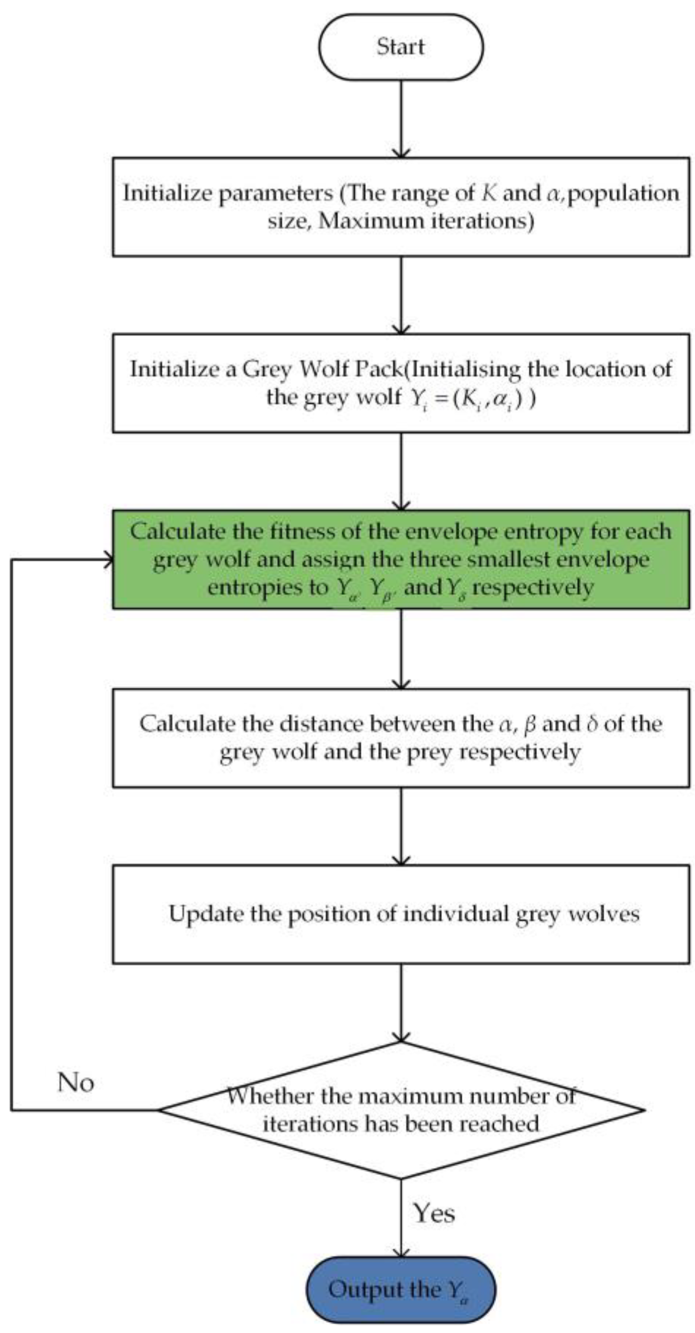
The flowchart of IVMD is shown in Figure 1, and the steps of IVMD are as follows:

(1)

Initialize the search space, encompass the ranges of $K$ and $\alpha$. Additionally, initiate the parameters of the grey wolf optimization algorithm, such as population size, maximum number of iterations, and so forth.

(2)

Generate the initial population of grey wolves randomly within the provided search space. For each grey wolf denoted by $i=1,2,\dots ,N$ (where $N$ represents the total number of grey wolves), the position $Y_i$ is initialized as ($K_i$, ${\alpha }_i$).

(3)

Calculate the envelope entropy of each grey wolf with Equation (22). The positions of the three grey wolves with the lowest envelope entropy values are updated by $Y_{\alpha }$, $Y_{\beta }$, and $Y_{\delta }$, respectively. $Y_{\alpha }$ with the best fitness value is recognized as the optimal solution.

(4)

Compute the distance between the remaining grey wolf individuals ($\omega$) and the top three grey wolf individual locations $Y_{\alpha }$, $Y_{\beta }$ and $Y_{\delta }$ according to Equations (15)–(17).

(5)

According to Equations (18)–(21), update the position of individual grey wolves.

(6)

If the iteration of GWO reaches maximum, the algorithm ends and outputs an optimal solution $Y_{\alpha }$; otherwise, return to (3) and continue the optimization search.

2.5. DLinear

DLinear is a novel high-precision time-series forecasting model proposed by Zeng et al. in 2022 [27]. Despite its simple structure, consisting solely of a decomposition scheme and two linear networks, its predictive accuracy exceeds that of the more complex transformer model.

During the prediction process, the DLinear first decomposes the original sequence $X$ into a trend component $X_t$ and a residual one ${\mathrm{X}}_r(X_r=X-X_t)$. Subsequently, two single-layer linear networks are utilized to forecast each of these decomposed components, respectively.

The foundational architecture of DLinear is depicted in Figure 2a. The output results of the two single-layer linear networks are combined to yield the final predicted outcome $\widehat{X}$ [27].

$$H_r=W_r{X}_r$$

(26)

$$H_t=W_t{X}_t$$

(27)

$$\widehat{X}=H_t+H_r$$

(28)

where $H_r$ and $H_t$ are the output values of the single-layer linear networks for the residual and trend components, respectively. Similarly, $W_r$ and $W_t$ represent the single-layer linear networks for the residual and the trend components, as depicted in Figure 2b.

2.6. Framework of the Proposed Model

The HI-IVMD-DLinear model is designed to achieve accurate multi-step WSF. The basic framework of this hybrid WSF model is illustrated in Figure 3, which mainly consists of three steps as follows:

Step 1: Outlier detection and replacement based on HI. Due to equipment malfunctions, human factors, and other reasons, it is inevitable that the collected wind speed data will contain outliers during the data collection process. The HI method is used to detect and replace outliers in the dataset, which is beneficial to improve the accuracy of WSF.

Step 2: Decomposition of wind speed sequences. The sequence processed by the HI is considered as input for the VMD. The GWO is then employed to optimize the hyperparameters $K$ and $\alpha$ of the VMD with the minimal envelope entropy as the fitness function. Based on the optimized values of $K$ and $\alpha$, the VMD decomposes the sequence into $K$ IMFs.

Step 3: Prediction with DLinear. The DLinear model is constructed to predict each of the $K$ IMFs obtained from the decomposition. Subsequently, the predicted results are summed to derive the ultimate wind speed prediction.

3. Results

3.1. Design of the Experiment

3.1.1. Data Source

The historical wind speed datasets collected from three regions in China serve as the experimental dataset. These three regions are, respectively, located in Shijiazhuang, Hebei Province; Lanzhou, Gansu Province; and Nanjing, Jiangsu Province. Their latitudes and longitudes are significantly different. Lanzhou and Shijiazhuang are situated in the northwestern and northern inland regions, respectively, both possessing abundant wind energy resources. On the other hand, Nanjing is located in the southeastern coastal area and consistently ranks among the top in terms of offshore wind power installed capacity nationwide. The wind speed sequences from all three regions were measured at a height of ten meters above ground level at hourly intervals. The basic information of the three wind speed datasets is presented in

Table 1. Basic information of three datasets.

Dataset	Time Interval	Sample Size	Minimum	Mean	Maximum	Standard Deviation
Lanzhou	1 January 2021–31 March 2021	2160	0.000	1.830	6.765	1.317
Nanjing	1 August 2021–1 November 2021	2232	0.000	2.849	7.657	1.705
Shijiazhuang	1 July 2021–1 October 2021	2232	0.000	1.844	6.408	1.585

.

3.1.2. Evaluation Metrics

To evaluate the accuracy of the prediction methods, the mean absolute error (MAE), root mean square error (RMSE), and mean absolute percentage error (MAPE) are employed

$$\mathrm{MAE}=\frac{1}{N}{\displaystyle \sum _{t=1}^N\left|{\widehat{Y}}_t-Y_t\right|}$$

(29)

$$\mathrm{RMSE}=\sqrt{\frac{1}{N}{\displaystyle \sum _{t=1}^N{\left({\widehat{Y}}_t-Y_t\right)}^2}}$$

(30)

$$\mathrm{MAPE}=\frac{{\displaystyle \sum _{t=1}^N\left|\frac{{\widehat{Y}}_t-Y_t}{Y_t}\right|}}{N}\times 100\%$$

(31)

where ${\widehat{Y}}_t$ represents the predicted value of the wind speed, $Y_t$ represents the observed value, and $N$ refers to the number of test-set samples. Generally speaking, as the values of these metrics decrease, the prediction accuracy of the model increases.

Furthermore, improvement percentage is utilized to quantitatively evaluate the proposed model. $P_{\mathrm{RMSE}}$, $P_{\mathrm{MAE}}$, and $P_{\mathrm{MAPE}}$ are the improvement percentages for RMSE, MAE, and MAPE, respectively.

$${\mathrm{P}}_{\mathrm{RMSE}}=\frac{{\mathrm{RMSE}}_i-{\mathrm{RMSE}}_j}{{\mathrm{RMSE}}_i}\times 100\%$$

(32)

$$P_{\mathrm{MAE}}=\frac{{\mathrm{MAE}}_i-{\mathrm{MAE}}_j}{{\mathrm{MAE}}_i}\times 100\%$$

(33)

$$P_{\mathrm{MAPE}}=\frac{{\mathrm{MAPE}}_i-{\mathrm{MAPE}}_j}{{\mathrm{MAPE}}_i}\times 100\%$$

(34)

where ${\mathrm{RMSE}}_i$, ${\mathrm{MAE}}_i$, and ${\mathrm{MAPE}}_i$ represent the errors of the comparative methods, while ${\mathrm{RMSE}}_j$, ${\mathrm{MAE}}_j$, and ${\mathrm{MAPE}}_j$ represent the errors of the HI-IVMD-DLinear method. The larger the $P_{\mathrm{RMSE}}$, $P_{\mathrm{MAE}}$, and $P_{\mathrm{MAPE}}$ are, the more superior the precision of the proposed model is.

In addition, the variance of absolute error (VAE) is introduced to assess the stability of the model.

$$\mathrm{VAE}=\mathrm{Var}\left(\left|{\mathrm{Y}}_t-{\widehat{Y}}_t\right|\right)$$

(35)

Simultaneously, the improvement percentage of $\mathrm{VAE}$ is also introduced to compare the proposed model with the comparative model.

$$P_{\mathrm{VAE}}=\frac{{\mathrm{VAE}}_i-{\mathrm{VAE}}_j}{{\mathrm{VAE}}_i}\times 100\%$$

(36)

where ${\mathrm{VAE}}_i$ and ${\mathrm{VAE}}_j$ represent the $\mathrm{VAE}$ of the comparative model and the proposed one, respectively.

3.1.3. Model Development

To assess the performance of HI-IVMD-DLinear, a machine learning model, SVR, two prevalent neural network models, namely, back propagation neural network (BPNN) and LSTM, as well as a popular deep learning algorithm, the transformer, are incorporated as comparative models.

The input for predicting the output values includes the true values from the previous 24 h; i.e., the time window size is 24 h.

Table 2. Parameters of all related methods.

Methods	Parameters	Values
IVMD	Population size	50
	Maximum iterations	30
	$K$	[3, 11]
	$\alpha$	[0, 1000]
SVR	C	[0, 10]
	Epsilon	[0, 1]
	Gamma	[0, 2]
BPNN	Dropout	[0.05, 0.2]
	Batchsize	64
	Epochs	100
	Initial lr	0.1
	Hidden_units	[10, 100]
LSTM	Dropout	[0.05, 0.2]
	Batchsize	64
	Epochs	100
	Initial lr	0.1
	Hidden_units	[10, 100]
Transformer	Dropout	[0.05, 0.2]
	Batchsize	64
	Epochs	100
	Initial lr	0.1
	Model dimension	[64, 256]
	Feedforward dimension	[128, 256]
	Heads number	[1, 5]
	Enc_layers	[1, 5]
	Dec_layers	[1, 5]
DLinear	Batchsize	64
	Epochs	100
	Initial lr	0.1

provides the parameter settings for all relevant models, along with the methods used to confirm these parameters. The dataset is divided into training, validation, and testing sets at a ratio of 7:1:2. Additionally, all models employ mean squared error (MSE) as the loss function. To optimize the weights and enhance the prediction performance, the Adam algorithm is employed as an optimizer [52].

3.2. Analysis of Hampel Identifier

The performance of utilizing HI for the data cleaning of the wind speed sequence is explored in this section. As illustrated in Figure 4, all three wind speed datasets exhibit some outliers. Failure to clean these outliers would adversely impact the accuracy of the final WSF. Therefore, the HI method can be utilized to handle the outliers in the wind speed sequences. The effectiveness of the HI can generally be evaluated by calculating the sample entropy of the sequences. The magnitude of the SampEn value reflects the complexity of the sequence [48]. If the complexity of the sequence is greater, the SampEn value will be larger, and vice versa. The SampEn values of the original wind speed sequences and the HI-processed wind speed sequences are presented in

Table 3. The SampEn value of original and HI-processed datasets.

SampEn	Lanzhou	Nanjing	Shijiazhuang
Original sequence	1.0562	1.0230	1.0658
Sequence after HI	1.0497	0.9534	0.9570

. It is evident that the SampEn values of all three wind speed sequences are reduced after applying the HI method. It indicates that the HI method can reduce the complexity of the original sequences.

The predictive performances of models with and without HI are also compared.

Table 4. Improvement percentages with HI.

Dataset	Model	PMAE (%)	PRMSE (%)	PMAPE (%)
Lanzhou	HI-SVR vs. SVR	2.1206	4.1472	2.5125
	HI-LSTM vs. LSTM	1.2452	3.5612	2.0106
	HI-Transformer vs. Transformer	0.8921	3.5125	2.2215
	HI-DLinear vs. DLinear	0.9915	1.1305	1.7683
	HI-IVMD-DLinear vs. IVMD-DLinear	0.7624	1.0614	1.2316
Nanjing	HI-SVR vs. SVR	1.5125	3.8903	1.7246
	HI-LSTM vs. LSTM	2.2092	5.2137	3.0165
	HI-Transformer vs. Transformer	1.2875	5.1751	3.1062
	HI-DLinear vs. DLinear	2.1785	2.1867	2.1554
	HI-IVMD-DLinear vs. IVMD-DLinear	1.0126	1.8751	2.1240
Shijiazhuang	HI-SVR vs. SVR	3.5613	3.1451	6.1246
	HI-LSTM vs. LSTM	2.5146	0.8915	4.1256
	HI-Transformer vs. Transformer	1.8745	1.3271	4.6012
	HI-DLinear vs. DLinear	2.0761	1.0512	3.1251
	HI-IVMD-DLinear vs. IVMD-DLinear	1.5612	0.7951	2.1531

gives the forecasting accuracy of models with HI processing and without HI processing under the three datasets. It can be observed that the improvement percentages of MAPE are 1.2316%, 2.1240%, and 2.1531% compared with the HI-IVMD-DLinear with IVMD-DLinear, respectively. Other HI-based models also reduce the RMSE, MAE, and MAPE values. Therfore the HI can enhance the accuracy of WSF, since HI is able to identify and rectify outliers in the original wind speed sequence, which can efficiently mitigate the interference caused by such outliers.

3.3. Decomposition Results

According to the augmented Dickey–Fuller (ADF) test results presented in

Table 5. ADF test results.

Datasets	t-Statistic	p-Value	1% Level	5% Level	10% Level
Lanzhou	−1.714	0.3704	−3.2334	−2.6828	−2.3674
Nanjing	−1.227	0.5513	−2.8910	−2.2150	−1.9674
Shijiazhuang	−1.827	0.3207	−3.3517	−2.7124	−2.4512

, the ADF statistics of the three datasets, after undergoing HI processing, are all below the critical values at the 1%, 5%, and 10% confidence levels. Additionally, their p-values are greater than 0.1. It is evident that the three wind speed sequences are non-stationary. Hence, it is imperative to decompose the wind speed sequences appropriately to reduce their complexity. The parameters of VMD are optimized by the GWO. The obtained hyperparameters $K$ and $\alpha$ for VMD on the three datasets are 4 and 1.2771, 4 and 0.4501, 5 and 0.2580, respectively.

Taking Lanzhou as an example, the decomposition results of the wind speed sequence, after undergoing HI processing, are illustrated in Figure 5a. IVMD decomposes the sequence of Lanzhou into four IMFs. Among them, IMF1 has the lowest frequency and displays the long-term trend of the wind speed sequence. IMF2 and IMF3 belong to the mid-frequency range signals, reflecting the fluctuations within smaller periods. IMF4 represents the high-frequency range signal. Evidently, the sequence exhibits a more regular pattern after the IVMD decomposition.

3.4. Forecasting Results

The HI-processed dataset is utilized for IVMD decomposition, with the subsequent prediction of each modal component with DLinear. Summing the predicted outcomes of these components yields the final WSF. Specifically, during training, only the training set should undergo decomposition, ensuring the data in the test set remain unknown. This safeguards against the inflated accuracy resulting from test set leakage. Subsequently, the IMFs derived from the training set decomposition are employed to train the model, while hyperparameter selection is performed on the validation set. Finally, test is conducted on the designated subsequence of the complete dataset. To assess the performance of the HI-IVMD-DLinear, HI-SVR, HI-BPNN, HI-LSTM, HI-Transformer, HI-DLinear, HI-IVMD-BPNN, HI-IVMD-LSTM, and HI-IVMD-Transformer are considered.

During the process of WSF, it is important to forecast wind speeds for multiple hours in advance. For instance, multi-step WSF assists wind power generation companies in accurately anticipating changes in wind speed over a specific period. This enables them to devise more efficient power generation plans and scheduling strategies to enhance the capacity and the efficiency of wind power generation. Therefore, the introduction of multi-step WSF is crucial. Given the wind speed sequence $\{Y_1,{\mathrm{Y}}_2,Y_3,\dots ,Y_T\}$, the forecasting value for the $k-\mathrm{th}$ step can be calculated as

$${\widehat{Y}}_{t+k}=f\left(Y_t,Y_{t-1},\dots ,Y_{t-(w-1)}\right),t=1,2,\dots ,T$$

(37)

where ${\widehat{Y}}_{t+k}$ represents the predicted value at time $t+k$, $Y_t$ represents the observed value at time $t$, and $w$ refers to the lag order. The value of $w$ is set as 24, in other words, the model takes the past 24 h wind speed sequence as its input. The horizon $k$ ranges from 1 to 4.

3.4.1. Forecasting Accuracy

The forecasting results of three metrics for HI-IVMD-DLinear and other comparative models are presented in

Table 6. Results of three evaluation metrics of multi-step-ahead prediction in Lanzhou.

Estimation Horizon	Metric	HI-SVR	HI-BPNN	HI-LSTM	HI-Transformer	HI-DLinear	HI-IVMD-BPNN	HI-IVMD-LSTM	HI-IVMD-Transformer	HI-IVMD-DLinear
1-step	MAE	0.3179	0.2773	0.2689	0.2366	0.2064	0.1688	0.1213	0.0767	0.0501
	RMSE	0.4116	0.3750	0.3592	0.3261	0.2582	0.2038	0.1452	0.1069	0.0641
	MAPE	0.1535	0.1494	0.1362	0.1213	0.1023	0.0745	0.0700	0.0421	0.0237
2-step	MAE	0.4391	0.4380	0.3345	0.3301	0.2826	0.2273	0.2025	0.1512	0.1207
	RMSE	0.6031	0.5832	0.4533	0.4426	0.3779	0.3152	0.2898	0.2124	0.1578
	MAPE	0.2240	0.2251	0.1785	0.1844	0.1596	0.1223	0.1065	0.0814	0.0601
3-step	MAE	0.4512	0.4405	0.385	0.3816	0.3434	0.2877	0.2587	0.2223	0.1398
	RMSE	0.6001	0.5813	0.5164	0.5173	0.4567	0.4045	0.3649	0.2882	0.1909
	MAPE	0.2356	0.2304	0.212	0.2098	0.1799	0.1765	0.1528	0.1103	0.0687
4-step	MAE	0.5240	0.5114	0.4412	0.4133	0.3713	0.3437	0.3381	0.2512	0.1666
	RMSE	0.6861	0.6732	0.5942	0.5559	0.4898	0.4125	0.3538	0.3051	0.2136
	MAPE	0.2523	0.2581	0.2345	0.2295	0.2034	0.2010	0.1782	0.1312	0.0839

,

Table 7. Results of three evaluation metrics of multi-step-ahead prediction in Nanjing.

Estimation Horizon	Metric	HI-SVR	HI-BPNN	HI-LSTM	HI-Transformer	HI-DLinear	HI-IVMD-BPNN	HI-IVMD-LSTM	HI-IVMD-Transformer	HI-IVMD-DLinear
1-step	MAE	0.4463	0.4080	0.3691	0.3572	0.3295	0.1325	0.1152	0.0911	0.0705
	RMSE	0.5533	0.5324	0.471	0.4694	0.4332	0.1668	0.1472	0.1253	0.0881
	MAPE	0.3839	0.3082	0.292	0.2705	0.2418	0.0917	0.0792	0.0632	0.0479
2-step	MAE	0.5244	0.5035	0.4785	0.4696	0.3797	0.2258	0.208	0.1717	0.1113
	RMSE	0.6814	0.6615	0.6172	0.6118	0.4699	0.2989	0.2752	0.229	0.1477
	MAPE	0.4356	0.4045	0.3905	0.3766	0.2557	0.1562	0.1511	0.1118	0.0773
3-step	MAE	0.5724	0.5620	0.5368	0.5304	0.4531	0.2592	0.211	0.1871	0.1381
	RMSE	0.7621	0.7394	0.6977	0.7005	0.6014	0.3488	0.3001	0.2624	0.1834
	MAPE	0.4761	0.4300	0.4477	0.4459	0.3346	0.1825	0.1629	0.1412	0.0956
4-step	MAE	0.6348	0.6034	0.5716	0.5615	0.4495	0.3071	0.2509	0.2215	0.1648
	RMSE	0.8500	0.8108	0.7718	0.7457	0.6271	0.4024	0.3583	0.2918	0.2289
	MAPE	0.5298	0.5009	0.4826	0.4682	0.3532	0.2206	0.2012	0.1811	0.1266

and

Table 8. Results of three evaluation metrics of multi-step-ahead prediction in Shijiazhuang.

Estimation Horizon	Metric	HI-SVR	HI-BPNN	HI-LSTM	HI-Transformer	HI-DLinear	HI-IVMD-BPNN	HI-IVMD-LSTM	HI-IVMD-Transformer	HI-IVMD-DLinear
1-step	MAE	0.3073	0.3041	0.2697	0.2540	0.2060	0.1441	0.1277	0.0939	0.0669
	RMSE	0.3937	0.3908	0.3564	0.3383	0.2847	0.2013	0.1765	0.1283	0.0861
	MAPE	0.2506	0.2281	0.1935	0.1936	0.1510	0.1225	0.1022	0.0661	0.0480
2-step	MAE	0.4121	0.4139	0.4026	0.3745	0.2976	0.2255	0.1768	0.1202	0.0814
	RMSE	0.5261	0.5286	0.5188	0.5040	0.3945	0.3132	0.2371	0.1612	0.1054
	MAPE	0.2799	0.2823	0.3379	0.2642	0.2215	0.1946	0.1268	0.0912	0.0569
3-step	MAE	0.4625	0.4574	0.4396	0.3995	0.3246	0.2752	0.2248	0.1512	0.1000
	RMSE	0.6031	0.5997	0.5657	0.5401	0.4224	0.3674	0.2903	0.2342	0.1338
	MAPE	0.3412	0.3275	0.3392	0.3114	0.2551	0.2157	0.1735	0.1023	0.0690
4-step	MAE	0.4951	0.4941	0.4871	0.4519	0.3814	0.3502	0.2861	0.2215	0.1439
	RMSE	0.6431	0.6335	0.6195	0.5761	0.4745	0.4264	0.3683	0.3012	0.2141
	MAPE	0.3620	0.3639	0.3530	0.3614	0.3095	0.2849	0.2543	0.2202	0.1023

. In all three datasets, the HI-IVMD-DLinear model outperforms the others in terms of MAE, RMSE, and MAPE. The HI-IVMD-DLinear exhibits the best predictive accuracy among the comparative models and is better suitable for the WSF task.

Taking Lanzhou as an example, compared with other models, the HI-IVMD-DLinear model achieves lower MAE, RMSE, and MAPE values. The MAE, RMSE, and MAPE values for the HI-IVMD-DLinear’s one-step-ahead prediction are 0.0705, 0.0881, and 0.0479, respectively, which are smaller than those of other models. Specifically, the MAPE values for HI-SVR, HI-BPNN, HI-LSTM, HI-Transformer, HI-DLinear, HI-IVMD-BPNN, HI-IVMD-LSTM, HI-IVMD-Transformer, and HI-IVMD-DLinear are 0.3839, 0.3082, 0.2920, 0.2705, 0.2418, 0.0917, 0.0792, 0.0632, and 0.0479, respectively. Among them, the HI-IVMD-DLinear achieves the smallest MAPE value. Moreover, for one-step-ahead to four-steps-ahead predictions, the HI-IVMD-DLinear obtains the optimal MAPE values of 0.0773, 0.0956, and 0.1266, respectively. Additionally, the HI-IVMD-DLinear also obtains the best MAE and RMSE values.

Furthermore, according to Table 6, Table 7 and Table 8, it is evident that the hybrid methods based on IVMD outperform the individual models in terms of accuracy. Taking the one-step-ahead forecasting in Lanzhou as an example, the MAPE value of the HI-DLinear is 0.2418, while that of the HI-IVMD-DLinear is 0.0479. Therefore the IVMD method helps diminish the complexity of the wind speed series enables the forecasting model to capture valuable patterns within the wind speed series, and effectively improves the forecasting performance.

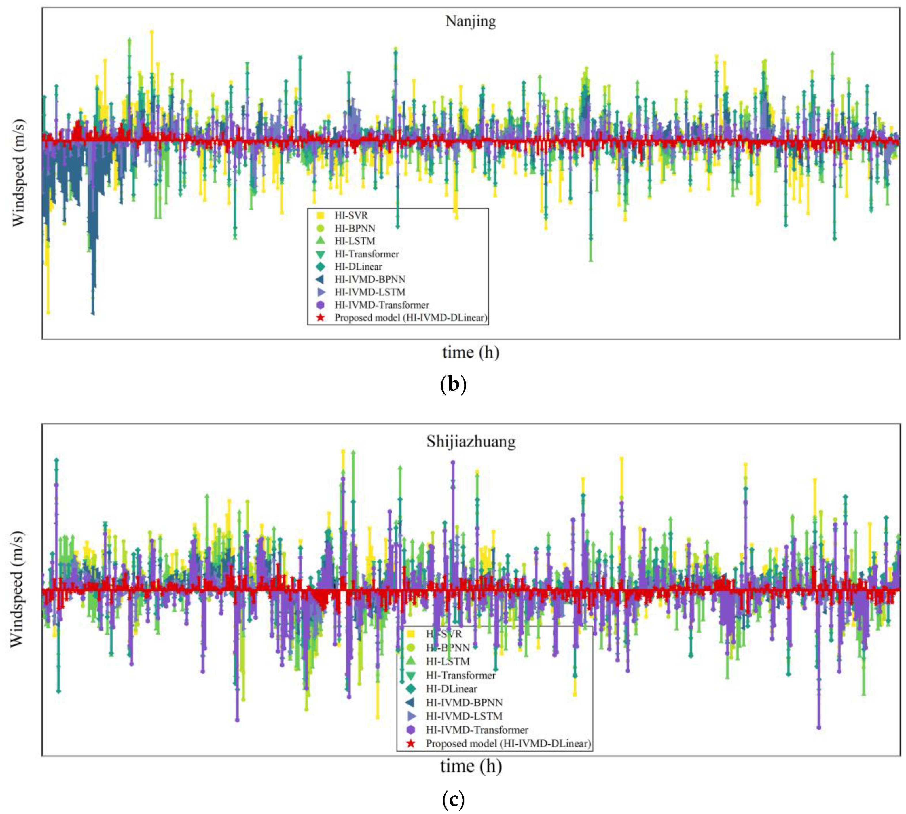
The comparison between the predicted and the observed wind speed values in the three datasets is illustrated in Figure 6. It can be observed that the prediction curve of the HI-IVMD-DLinear hybrid model closely resembles that of the observed wind speed values. This highlights better predictive accuracy of the HI-IVMD-DLinear model in the field of WSF than other comparative models.

Meanwhile, compared with the individual HI-SVR, HI-BPNN, HI-LSTM, HI-Transformer, and HI-DLinear models, the prediction curves of HI-IVMD-SVR, HI-IVMD-BPNN, HI-IVMD-LSTM, HI-IVMD-Transformer, and HI-IVMD-DLinear across the three datasets exhibit a higher degree of similarity to the observed wind speed curves. Thus the IVMD decomposition is helpful in WSF.

3.4.2. Improvement Percentage in Accuracy

The improvement percentages of accuracy metrics for the HI-IVMD-DLinear model are presented in

Table 9. Improvement percentages on three metrics of HI-IVMD-DLinear compared with comparable models in Lanzhou.

Estimation Horizon	Metric	HI-SVR	HI-BPNN	HI-LSTM	HI-Transformer	HI-DLinear	HI-IVMD-BPNN	HI-IVMD-LSTM	HI-IVMD-Transformer
1-step	PMAE (%)	84.2033	82.7196	80.9005	80.2659	78.6032	46.7841	38.8104	22.6125
	PRMSE (%)	84.0766	83.4535	81.2947	81.2296	79.6612	47.1681	40.1372	29.6887
	PMAPE (%)	87.5236	84.4584	83.5969	82.2938	80.1936	47.7605	39.5475	24.2089
2-step	PMAE (%)	78.7740	77.8952	76.7398	76.3006	70.6891	50.7040	46.4791	35.1776
	PRMSE (%)	78.3228	77.6722	76.0693	75.8583	68.5685	50.5914	46.3353	35.5022
	PMAPE (%)	82.2549	80.8899	80.2049	79.4739	69.7645	50.5266	48.8467	30.8587
3-step	PMAE (%)	75.8735	75.4275	74.2732	73.9633	69.5241	46.7304	34.5396	26.1892
	PRMSE (%)	75.9363	75.1968	73.7148	73.8202	69.5041	47.4129	38.8968	30.1067
	PMAPE (%)	79.9212	77.7699	78.6447	78.5622	71.4304	47.6040	41.3313	32.2946
4-step	PMAE (%)	74.0380	72.6866	71.1707	70.6518	63.3334	46.3339	34.3082	25.5982
	PRMSE (%)	73.0713	71.7671	70.3405	69.3023	63.4987	43.1154	36.1221	21.5559
	PMAPE (%)	76.1047	74.7235	73.7673	72.9588	64.1566	42.6058	37.0858	30.0939

,

Table 10. Improvement percentages on three metrics of HI-IVMD-DLinear compared with comparable models in Nanjing.

Estimation Horizon	Metric	HI-SVR	HI-BPNN	HI-LSTM	HI-Transformer	HI-DLinear	HI-IVMD-BPNN	HI-IVMD-LSTM	HI-IVMD-Transformer
1-step	PMAE (%)	84.2409	81.9333	81.3657	78.8260	75.7224	70.3199	58.6831	34.6806
	PRMSE (%)	84.4272	82.9060	82.1564	80.3460	75.1727	68.5442	55.8529	40.0374
	PMAPE (%)	84.5591	84.1313	82.5998	80.4556	76.8356	68.1678	66.1645	43.7055
2-step	PMAE (%)	72.5134	72.4446	63.9205	63.4358	57.2882	46.8873	40.3826	20.1904
	PRMSE (%)	73.8362	72.9428	65.1858	64.3458	58.2394	49.9432	45.5538	25.6908
	PMAPE (%)	73.1711	73.2950	66.3302	67.4084	62.3519	50.8716	43.5630	26.1879
3-step	PMAE (%)	69.0184	68.2667	63.6840	63.3623	59.2891	51.4043	45.9572	37.1233
	PRMSE (%)	68.1908	67.1616	63.0349	63.0957	58.1990	52.8060	47.6892	33.7700
	PMAPE (%)	70.8416	70.1822	67.5903	67.2581	61.8191	61.0778	55.0276	37.7379
4-step	PMAE (%)	68.2063	67.4222	62.2392	59.6876	55.1269	51.5240	50.7219	33.6865
	PRMSE (%)	68.8684	68.2711	64.0548	61.5750	56.3870	48.2202	39.6268	29.9954
	PMAPE (%)	66.7518	67.4935	64.2221	63.4508	58.7554	58.2622	52.9276	36.0750

and

Table 11. Improvement percentages on three metrics of HI-IVMD-DLinear compared with comparable models in Shijiazhuang.

Estimation Horizon	Metric	HI-SVR	HI-BPNN	HI-LSTM	HI-Transformer	HI-DLinear	HI-IVMD-BPNN	HI-IVMD-LSTM	HI-IVMD-Transformer
1-step	PMAE (%)	78.2167	77.99	75.18	73.65	67.50	53.54	47.59	28.72
	PRMSE (%)	78.1334	77.97	75.84	74.55	69.76	57.24	51.21	32.90
	PMAPE (%)	80.8590	78.98	75.22	75.23	68.24	60.86	53.09	27.44
2-step	PMAE (%)	80.2491	80.33	79.78	78.26	72.65	63.90	53.96	32.25
	PRMSE (%)	79.9665	80.06	79.68	79.09	73.28	66.35	55.54	34.62
	PMAPE (%)	79.6722	79.84	83.16	78.46	74.31	70.77	55.11	37.63
3-step	PMAE (%)	78.3790	78.14	77.25	74.97	69.19	63.66	55.51	33.88
	PRMSE (%)	77.8146	77.69	76.35	75.23	68.32	63.59	53.91	42.88
	PMAPE (%)	79.7793	78.93	79.66	77.84	72.96	68.01	60.22	32.56
4-step	PMAE (%)	70.9363	70.87	70.46	68.16	62.27	58.91	49.71	35.02
	PRMSE (%)	66.7056	66.20	65.44	62.84	54.88	49.79	41.87	28.93
	PMAPE (%)	71.7365	71.89	71.02	71.70	66.94	64.09	59.77	53.53

. It can be seen that the proposed model consistently achieves the lowest prediction errors across all four forecasting horizons on the three wind speed datasets. Thus the accuracy of the proposed model is acceptable.

As shown in Table 10, for the Nanjing dataset, the improvement percentages of MAPE for one-step-ahead prediction by the HI-IVMD-DLinear relative to HI-SVR, HI-BPNN, HI-LSTM, HI-Transformer, and HI-DLinear are 87.5236%, 84.4584%, 83.5969%, 82.2938%, and 80.1936% respectively. This indicates the necessity of decomposing the original sequence with IVMD in the WSF process.

Furthermore, like HI-IVMD-BPNN, HI-IVMD-LSTM, and HI-IVMD-Transformer, HI-IVMD-DLinear also demonstrates significantly higher prediction accuracy. As shown in Table 10, compared with HI-IVMD-BPNN, HI-IVMD-LSTM, and HI-IVMD-Transformer, the HI-IVMD-DLinear exhibits improvement percentages 58.2622%, 52.9276%, and 36.0750% in MAPE for the one-step-ahead and two-steps-ahead predictions, respectively.

Therefore the HI-IVMD-DLinear outperforms the other models in the field of WSF in terms of accuracy.

3.4.3. Analysis of Forecasting Errors

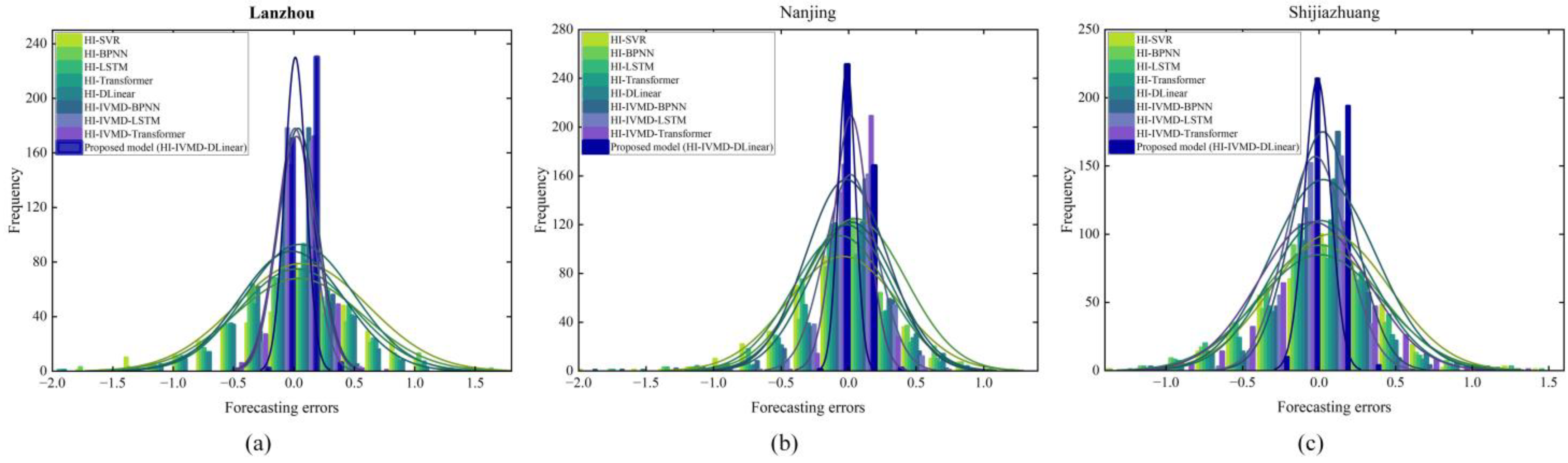
Figure 7 is the frequency distribution of the predictive errors with the proposed model and eight other comparative models, regarding one-step-ahead predictions. The graph indicates that the error of the model based on the IVMD is small. Additionally, it can be observed that the HI-IVMD-DLinear presents the smallest errors among the majority of the data points in the test set.

Figure 8 illustrates the distribution of errors for each model. It is noticeable that the HI-IVMD-DLinear exhibits a higher concentration of prediction errors around zero for each dataset than the other models, with a smaller range of error variation. This implies that the HI-IVMD-DLinear possesses exceptional predictive accuracy and robustness.

3.4.4. Stability Analysis

Table 12. Predictive stability results (VAE) in three datasets.

Estimation Horizon	HI-SVR	HI-BPNN	HI-LSTM	HI-Transformer	HI-DLinear	HI-IVMD-BPNN	HI-IVMD-LSTM	HI-IVMD-Transformer	HI-IVMD-DLinear
Lanzhou
1-step	0.1200	0.1100	0.0893	0.1102	0.0513	0.0197	0.0129	0.0211	0.0028
2-step	0.1920	0.1890	0.1541	0.1899	0.1127	0.0383	0.0313	0.0316	0.0084
3-step	0.2112	0.2216	0.1873	0.2012	0.1577	0.0512	0.0544	0.0412	0.0178
4-step	0.2635	0.2539	0.2367	0.2524	0.2025	0.0551	0.0676	0.0518	0.0264
Nanjing
1-step	0.0667	0.0571	0.0536	0.0610	0.0506	0.0327	0.0114	0.0110	0.0052
2-step	0.1098	0.0835	0.0997	0.0811	0.0710	0.0477	0.0327	0.0411	0.0173
3-step	0.1371	0.1380	0.1178	0.1225	0.1048	0.0902	0.0669	0.0624	0.0353
4-step	0.1620	0.1610	0.1503	0.1503	0.1303	0.1333	0.1047	0.1009	0.0603
Shijiazhuang
1-step	0.0651	0.0610	0.0652	0.0782	0.0514	0.0137	0.0100	0.0416	0.0044
2-step	0.1021	0.1019	0.0922	0.0956	0.0781	0.0412	0.0266	0.0210	0.0096
3-step	0.1241	0.1221	0.1170	0.1018	0.0921	0.0810	0.0591	0.0411	0.0336
4-step	0.1407	0.1395	0.1301	0.1312	0.1139	0.1065	0.0872	0.0721	0.0655

is the variance of absolute errors (VAE) with the proposed model and all comparative models across three datasets for multi-step ahead predictions. It reveals that the proposed model has good stability since it obtains the lowest VAE for one-to-four-steps-ahead predictions across all three datasets. For instance, in the Lanzhou dataset, the HI-IVMD-DLinear achieves VAE values of 0.0028, 0.0084, 0.0178, and 0.0264 for one-to-four-steps-ahead predictions, respectively. These values are consistently lower than those of the other comparative models.

The improvement percentages of VAE for the HI-IVMD-DLinear together with other comparative models are depicted in Figure 9. Compared to HI-SVR, HI-BPNN, HI-LSTM, HI-Transformer, and HI-DLinear, the HI-IVMD-DLinear exhibits a reduction in VAE of over 50% under the three datasets,. The IVMD decomposition also enhances the stability of predictions. Furthermore, compared to HI-IVMD-BPNN, HI-IVMD-LSTM, and HI-IVMD-Transformer, the HI-IVMD-DLinear achieves a reduction in VAE ranging from 9.0707% to 85.8084%. Hence, the DLinear-based model is more stable than BPNN, LSTM, and transformer.

3.5. Comparative Analysis of Decomposition Strategies

To validate the decomposition performance of IVMD, IVMD is compared with the decomposition strategies including EMD [53], CEEMDAN [37], and the recently published CEEMDAN-VMD [54] and CEEMDAN-LMD [55]. Additionally, the strategy without decomposition methods is also compared. The CEEMDAN-VMD method begins by decomposing the wind speed sequence into several IMFs with CEEMDAN, followed by another decomposition of the highest-frequency IMF with VMD. Similarly, the CEEMDAN-LMD method involves decomposing the wind speed sequence into multiple IMFs with CEEMDAN, and subsequently decomposing the IMF1 generated from the CEEMDAN decomposition with LMD. The comparative results are presented in

Table 13. The RMSE in Lanzhou obtained by basic forecasting models combined with different decomposition strategies.

Strategy	SVR	BPNN	LSTM	Transformer	DLinear
Non-decomposition	0.5533	0.5324	0.4710	0.4694	0.4332
EMD	0.4119	0.3992	0.3611	0.3574	0.3192
CEEMDAN	0.3633	0.2731	0.2632	0.2427	0.174
CEEMDAN-VMD	0.3211	0.2031	0.1754	0.1641	0.1259
CEEMDAN-LMD	0.3275	0.1832	0.1618	0.1517	0.1187
IVMD	0.3015	0.1668	0.1472	0.1253	0.0881

.

• Based on the data presented in Table 13, the following conclusions can be inferred:

• Compared with the other decomposition strategies, the predictive models based on IVMD demonstrate the minimal RMSE values, specifically, 0.1712, 0.1668, 0.1472, 0.1253, and 0.0881. This further validates the superior performance of IVMD over the other decomposition strategies. CEEMDAN-VMD and CEEMDAN-LMD fail to address the inherent mode-mixing issue in the CEEMDAN algorithm, although they employ secondary decomposition, which reduces the complexity of sequences once again to some extent. This is why both have lower performance than IVMD.
• Compared to traditional machine learning methods like SVR, deep learning methods including BPNN, LSTM, transformer, and DLinear present significant improvement in predictive accuracy when combined with decomposition methods. For instance, the RMSE of IVMD-SVR and the SVR are 0.3015 and 0.5533, respectively. The RMSE is reduced by only 45.50% when incorporating IVMD. However, IVMD-DLinear and DLinear achieve an RMSE of 0.4332 and 0.0881, respectively. It is demonstrated that a remarkable RMSE reduction of 79.66% is achieved when combined with IVMD.
• For the same decomposition strategy, DLinear consistently obtains the lowest RMSE, implying DLinear generally has optimal accuracy.
• Among different combinations of decomposition strategies and original prediction models, IVMD-DLinear achieves the lowest RMSE of 0.0881. Therefore IVMD-DLinear has best predictive performance than the aforementioned combinations.

4. Discussion

WSF is a complex task influenced by various factors, such as temperature, humidity, and air pressure. These factors contribute to the non-stationary and nonlinear characteristics of wind speed sequences. It is challenging to forecast wind speeds with a single prediction model accurately. Precise WSF holds significant importance in the energy industry, as higher accuracy forecasts can help reduce operational costs of power systems.

4.1. Discussion of Computational Efficiency

In terms of computational efficiency, the proposed method outperforms the other prediction models. Specifically, the VMD allows for higher computational efficiency with distributed storage and parallel computing techniques, since each IMF’s prediction is independent of the others. Furthermore, the DLinear model has high efficiency, with each branch containing only a single linear layer. Significantly lower memory and fewer parameters are involved than the transformer, and faster calculation speeds.

4.2. Discussion of Computational Complexity

Compared with the other non-decomposition methods, the IVMD-DLinear increases the computational complexity within an acceptable range. The predictions for each IMF are obtained by applying the DLinear model to each IMF and the hyperparameter in VMD is optimized by the GWO algorithm, which significantly increases the computational complexity. However, it is reasonable since the substantial improvement in prediction accuracy augments the economic efficacy of wind power systems significantly.

5. Conclusions

Accurate and robust WSF is of great importance for the advancement of the wind power industry. Nevertheless, the intricate and non-stationary nature of wind speed sequences poses a significant challenge to achieve precise predictions. Therefore, a WSF model (HI-IVMD-DLinear) based on outlier correction, heuristic algorithms, and sequence decomposition is proposed to achieve high precision and robust wind speed forecasting. Firstly, the outliers in the wind speed sequence are detected and corrected with the outlier correction method HI to reduce the adverse effects of outliers on prediction accuracy. Secondly, the hyperparameters $K$ and $\alpha$ of the VMD are optimized by the GWO. Thirdly, with the optimized $K$ and $\alpha$, the wind speed sequence processed by HI is decomposed into several IMFs by the VMD, and the non-stationarity and the complexity of the sequence are reduced. Finally, each IMF is individually predicted by the novel DLinear algorithm, and the predicted outputs are summed to obtain the final wind speed prediction.

The experimental results conducted on wind speed datasets from three cities in China validate the predictive performance of the HI-IVMD-DLinear. Based on the experiments, the following conclusions can be drawn:

• HI assists in mitigating the detrimental effects of outliers on prediction accuracy, and enhances the overall precision of the predictions. HI can detect and correct outliers in wind speed series and reduce their interference in prediction.
• The IVMD algorithm demonstrates significant advantages compared to the EEMD, CEEMDAN, CEEMDAN-VMD, and CEEMDAN-LMD algorithms. The CEEMDAN algorithm shows spurious modes during decomposition, which can affect the accuracy of predictions to some extent. CEEMDAN-VMD and CEEMDAN-LMD fail to address the mode-mixing issue in CEEMDAN, although they employ secondary decomposition to reduce sequence complexity to some extent.
• The DLinear model has better optimal performance than the SVR, BPNN, LSTM, and transformer models. Simultaneously, DLinear is stable with higher prediction accuracy than that of the widely used and highly accurate transformer or LSTM models in the field of WSF, and it is not necessary to adjust its hyperparameters. Therefore, DLinear is more suitable for WSF than transformer and LSTM.
• In the one-to-four-steps-ahead forecasting on the three datasets, the HI-IVMD-DLinear model demonstrates excellent prediction accuracy compared with the other eight comparative models. This hybrid model utilizes HI for outlier correction, IVMD for sequence decomposition, and DLinear for prediction. The performance of the hybrid model has been validated at each stage.

Nevertheless, our study does possess certain limitations. Primarily, it relies heavily on simulations due to the current cost constraints that prevent us from conducting field measurements.

References

- Dong, F.; Li, W. Research on the Coupling Coordination Degree of “Upstream-Midstream-Downstream” of China’s Wind Power Industry Chain. J. Clean. Prod. 2021, 283, 124633. [Google Scholar] [CrossRef]
- World Wind Energy Association. Worldwide Wind Capacity Reaches 744 Gigawatts—An Unprecedented 93 Gigawatts Added in 2020; World Wind Energy Association: Bonn, Germany, 2021. [Google Scholar]
- Wang, L.; Li, J. Estimation of Extreme Wind Speed in SCS and NWP by a Non-Stationary Model. Theor. Appl. Mech. Lett. 2016, 6, 131–138. [Google Scholar] [CrossRef] [Green Version]
- Zhao, J.; Guo, Z.-H.; Su, Z.-Y.; Zhao, Z.-Y.; Xiao, X.; Liu, F. An Improved Multi-Step Forecasting Model Based on WRF Ensembles and Creative Fuzzy Systems for Wind Speed. Appl. Energy 2016, 162, 808–826. [Google Scholar] [CrossRef]
- Yang, J.; Astitha, M.; Delle Monache, L.; Alessandrini, S. An Analog Technique to Improve Storm Wind Speed Prediction Using a Dual NWP Model Approach. Mon. Weather. Rev. 2018, 146, 4057–4077. Available online: https://journals.ametsoc.org/view/journals/mwre/146/12/mwr-d-17-0198.1.xml (accessed on 30 April 2023). [CrossRef]
- Karakuş, O.; Kuruoğlu, E.E.; Altınkaya, M.A. One-day Ahead Wind Speed/Power Prediction Based on Polynomial Autoregressive Model. IET Renew. Power Gener. 2017, 11, 1430–1439. Available online: https://ietresearch.onlinelibrary.wiley.com/doi/10.1049/iet-rpg.2016.0972 (accessed on 30 April 2023). [CrossRef] [Green Version]
- Aasim; Singh, S.N.; Mohapatra, A. Repeated Wavelet Transform Based ARIMA Model for Very Short-Term Wind Speed Forecasting. Renew. Energy 2019, 136, 758–768. [Google Scholar] [CrossRef]
- Yatiyana, E.; Rajakaruna, S.; Ghosh, A. Wind Speed and Direction Forecasting for Wind Power Generation Using ARIMA Model. In Proceedings of the 2017 Australasian Universities Power Engineering Conference (AUPEC), Melbourne, Australia, 19–22 November 2017; pp. 1–6. [Google Scholar]
- Phan, Q.T.; Wu, Y.K.; Phan, Q.D. A Hybrid Wind Power Forecasting Model with XGBoost, Data Preprocessing Considering Different NWPs. Appl. Sci. 2021, 11, 1100. [Google Scholar] [CrossRef]
- Santamaría-Bonfil, G.; Reyes-Ballesteros, A.; Gershenson, C. Wind Speed Forecasting for Wind Farms: A Method Based on Support Vector Regression. Renew. Energy 2016, 85, 790–809. [Google Scholar] [CrossRef]
- Chen, J.; Zeng, G.-Q.; Zhou, W.; Du, W.; Lu, K.-D. Wind Speed Forecasting Using Nonlinear-Learning Ensemble of Deep Learning Time Series Prediction and Extremal Optimization. Energy Convers. Manag. 2018, 165, 681–695. [Google Scholar] [CrossRef]
- Wang, G.; Wang, X.; Wang, Z.; Ma, C.; Song, Z. A VMD–CISSA–LSSVM Based Electricity Load Forecasting Model. Mathematics 2021, 10, 28. [Google Scholar] [CrossRef]
- Ren, C.; An, N.; Wang, J.; Li, L.; Hu, B.; Shang, D. Optimal Parameters Selection for BP Neural Network Based on Particle Swarm Optimization: A Case Study of Wind Speed Forecasting. Knowl.-Based Syst. 2014, 56, 226–239. [Google Scholar] [CrossRef]
- Yang, Z.; Wang, J. A Hybrid Forecasting Approach Applied in Wind Speed Forecasting Based on a Data Processing Strategy and an Optimized Artificial Intelligence Algorithm. Energy 2018, 160, 87–100. [Google Scholar] [CrossRef]
- Wang, Z.; Wang, B.; Liu, C.; Wang, W. Improved BP Neural Network Algorithm to Wind Power Forecast. J. Eng. 2017, 2017, 940–943. [Google Scholar] [CrossRef]
- Duan, J.; Zuo, H.; Bai, Y.; Duan, J.; Chang, M.; Chen, B. Short-Term Wind Speed Forecasting Using Recurrent Neural Networks with Error Correction. Energy 2021, 217, 119397. [Google Scholar] [CrossRef]
- Gangwar, S.; Bali, V.; Kumar, A. Comparative Analysis of Wind Speed Forecasting Using LSTM and SVM. EAI Endorsed Trans. Scalable Inf. Syst. 2020, 7, e1. [Google Scholar] [CrossRef]
- Ying, X.; Zhao, K.; Liu, Z.; Gao, J.; He, D.; Li, X.; Xiong, W. Wind Speed Prediction via Collaborative Filtering on Virtual Edge Expanding Graphs. Mathematics 2022, 10, 1943. [Google Scholar] [CrossRef]
- Mousavi, S.M.; Ghasemi, M.; Dehghan Manshadi, M.; Mosavi, A. Deep Learning for Wave Energy Converter Modeling Using Long Short-Term Memory. Mathematics 2021, 9, 871. [Google Scholar] [CrossRef]
- Liu, H.; Mi, X.; Li, Y.; Duan, Z.; Xu, Y. Smart Wind Speed Deep Learning Based Multi-Step Forecasting Model Using Singular Spectrum Analysis, Convolutional Gated Recurrent Unit Network and Support Vector Regression. Renew. Energy 2019, 143, 842–854. [Google Scholar] [CrossRef]
- Xiang, L.; Li, J.; Hu, A.; Zhang, Y. Deterministic and Probabilistic Multi-Step Forecasting for Short-Term Wind Speed Based on Secondary Decomposition and a Deep Learning Method. Energy Convers. Manag. 2020, 220, 113098. [Google Scholar] [CrossRef]
- Zhang, G.; Liu, D. Causal Convolutional Gated Recurrent Unit Network with Multiple Decomposition Methods for Short-Term Wind Speed Forecasting. Energy Convers. Manag. 2020, 226, 113500. [Google Scholar] [CrossRef]
- Syu, Y.-D.; Wang, J.-C.; Chou, C.-Y.; Lin, M.-J.; Liang, W.-C.; Wu, L.-C.; Jiang, J.-A. Ultra-Short-Term Wind Speed Forecasting for Wind Power Based on Gated Recurrent Unit. In Proceedings of the 2020 8th International Electrical Engineering Congress (iEECON), Chiang Mai, Thailand, 4–6 March 2020; pp. 1–4. [Google Scholar]
- Wu, N.; Green, B.; Ben, X.; O’Banion, S. Deep Transformer Models for Time Series Forecasting: The Influenza Prevalence Case. arXiv 2020, arXiv:2001.08317. [Google Scholar]
- Bommidi, B.S.; Teeparthi, K.; Kosana, V. Hybrid Wind Speed Forecasting Using ICEEMDAN and Transformer Model with Novel Loss Function. Energy 2023, 265, 126383. [Google Scholar] [CrossRef]
- Wu, H.; Meng, K.; Fan, D.; Zhang, Z.; Liu, Q. Multistep Short-Term Wind Speed Forecasting Using Transformer. Energy 2022, 261, 125231. [Google Scholar] [CrossRef]
- Zeng, A.; Chen, M.; Zhang, L.; Xu, Q. Are Transformers Effective for Time Series Forecasting? arXiv 2022, arXiv:2205.13504. [Google Scholar]
- Büyükşahin, Ü.Ç.; Ertekin, Ş. Improving Forecasting Accuracy of Time Series Data Using a New ARIMA-ANN Hybrid Method and Empirical Mode Decomposition. Neurocomputing 2019, 361, 151–163. [Google Scholar] [CrossRef] [Green Version]
- Zhang, J.; Wei, Y.; Tan, Z. An Adaptive Hybrid Model for Short Term Wind Speed Forecasting. Energy 2020, 190, 115615. [Google Scholar] [CrossRef]
- Shang, Z.; He, Z.; Chen, Y.; Chen, Y.; Xu, M. Short-Term Wind Speed Forecasting System Based on Multivariate Time Series and Multi-Objective Optimization. Energy 2022, 238, 122024. [Google Scholar] [CrossRef]
- Liu, D.; Niu, D.; Wang, H.; Fan, L. Short-Term Wind Speed Forecasting Using Wavelet Transform and Support Vector Machines Optimized by Genetic Algorithm. Renew. Energy 2014, 62, 592–597. [Google Scholar] [CrossRef]
- Liu, H.; Mi, X.; Li, Y. Wind Speed Forecasting Method Based on Deep Learning Strategy Using Empirical Wavelet Transform, Long Short Term Memory Neural Network and Elman Neural Network. Energy Convers. Manag. 2018, 156, 498–514. [Google Scholar] [CrossRef]
- Wang, J.; Zhang, W.; Li, Y.; Wang, J.; Dang, Z. Forecasting Wind Speed Using Empirical Mode Decomposition and Elman Neural Network. Appl. Soft Comput. 2014, 23, 452–459. [Google Scholar] [CrossRef]
- Liu, H.; Chen, C.; Tian, H.; Li, Y. A Hybrid Model for Wind Speed Prediction Using Empirical Mode Decomposition and Artificial Neural Networks. Renew. Energy 2012, 48, 545–556. [Google Scholar] [CrossRef]
- A Complete Ensemble Empirical Mode Decomposition with Adaptive Noise. Available online: https://ieeexplore.ieee.org/document/5947265/ (accessed on 7 April 2023).
- Wang, S.; Zhang, N.; Wu, L.; Wang, Y. Wind Speed Forecasting Based on the Hybrid Ensemble Empirical Mode Decomposition and GA-BP Neural Network Method. Renew. Energy 2016, 94, 629–636. [Google Scholar] [CrossRef]
- Zhang, W.; Qu, Z.; Zhang, K.; Mao, W.; Ma, Y.; Fan, X. A Combined Model Based on CEEMDAN and Modified Flower Pollination Algorithm for Wind Speed Forecasting. Energy Convers. Manag. 2017, 136, 439–451. [Google Scholar] [CrossRef]
- Zhang, Y.; Pan, G.; Chen, B.; Han, J.; Zhao, Y.; Zhang, C. Short-Term Wind Speed Prediction Model Based on GA-ANN Improved by VMD. Renew. Energy 2020, 156, 1373–1388. [Google Scholar] [CrossRef]
- Li, Y.; Tang, B.; Jiao, S. SO-Slope Entropy Coupled with SVMD: A Novel Adaptive Feature Extraction Method for Ship-Radiated Noise. Ocean Eng. 2023, 280, 114677. [Google Scholar] [CrossRef]
- Liu, H.; Mi, X.; Li, Y. Smart Multi-Step Deep Learning Model for Wind Speed Forecasting Based on Variational Mode Decomposition, Singular Spectrum Analysis, LSTM Network and ELM. Energy Convers. Manag. 2018, 159, 54–64. [Google Scholar] [CrossRef]
- Mirjalili, S.; Mirjalili, S.M.; Lewis, A. Grey Wolf Optimizer. Adv. Eng. Softw. 2014, 69, 46–61. [Google Scholar] [CrossRef] [Green Version]
- Liu, H.; Xu, Y.; Chen, C. Improved Pollution Forecasting Hybrid Algorithms Based on the Ensemble Method. Appl. Math. Model. 2019, 73, 473–486. [Google Scholar] [CrossRef]
- Liu, H.; Shah, S.; Jiang, W. On-Line Outlier Detection and Data Cleaning. Comput. Chem. Eng. 2004, 28, 1635–1647. [Google Scholar] [CrossRef]
- Li, Y.; Geng, B.; Tang, B. Simplified Coded Dispersion Entropy: A Nonlinear Metric for Signal Analysis. Nonlinear Dyn. 2023, 111, 9327–9344. [Google Scholar] [CrossRef]
- Grassberger, P.; Procaccia, I. Characterization of Strange Attractors. Phys. Rev. Lett. 1983, 50, 346–349. [Google Scholar] [CrossRef]
- Li, Y.; Tang, B.; Geng, B.; Jiao, S. Fractional Order Fuzzy Dispersion Entropy and Its Application in Bearing Fault Diagnosis. Fractal Fract. 2022, 6, 544. [Google Scholar] [CrossRef]
- Zhu, K.; Song, X.; Xue, D. Fault Diagnosis of Rolling Bearings Based on IMF Envelope Sample Entropy and Support Vector Machine. J. Inf. Comput. Sci. 2013, 10, 5189–5198. [Google Scholar] [CrossRef]
- Chen, W.; Zhuang, J.; Yu, W.; Wang, Z. Measuring Complexity Using FuzzyEn, ApEn, and SampEn. Med. Eng. Phys. 2009, 31, 61–68. [Google Scholar] [CrossRef]
- Pearson, R.K. Outliers in Process Modeling and Identification. IEEE Trans. Control Syst. Technol. 2002, 10, 55–63. [Google Scholar] [CrossRef] [PubMed]
- Wang, J.; Du, P.; Hao, Y.; Ma, X.; Niu, T.; Yang, W. An Innovative Hybrid Model Based on Outlier Detection and Correction Algorithm and Heuristic Intelligent Optimization Algorithm for Daily Air Quality Index Forecasting. J. Environ. Manag. 2020, 255, 109855. [Google Scholar] [CrossRef]
- Dragomiretskiy, K.; Zosso, D. Variational Mode Decomposition. IEEE Trans. Signal Process. 2014, 62, 531–544. [Google Scholar] [CrossRef]
- Kingma, D.P.; Ba, J. Adam: A Method for Stochastic Optimization. arXiv 2017, arXiv:1412.6980. [Google Scholar]
- Huang, N.E.; Shen, Z.; Long, S.R.; Wu, M.C.; Shih, H.H.; Zheng, Q.; Yen, N.-C.; Tung, C.C.; Liu, H.H. The Empirical Mode Decomposition and the Hilbert Spectrum for Nonlinear and Non-Stationary Time Series Analysis. Proc. R. Soc. London. Ser. A Math. Phys. Eng. Sci. 1998, 454, 903–995. [Google Scholar] [CrossRef]
- Peng, T. Multi-Step Ahead Wind Speed Forecasting Using a Hybrid Model Based on Two-Stage Decomposition Technique and AdaBoost-Extreme Learning Machine. Energy Convers. Manag. 2017, 153, 589–602. [Google Scholar] [CrossRef]
- Emeksiz, C.; Tan, M. Multi-Step Wind Speed Forecasting and Hurst Analysis Using Novel Hybrid Secondary Decomposition Approach. Energy 2022, 238, 121764. [Google Scholar] [CrossRef]
Figure 1.
Flowchart of IVMD.
Figure 2.
Illustration of DLinear. (a): architecture of DLinear; (b): architecture of single-layer linear networks.
Figure 3.
The basic framework of HI-IVMD-DLinear model.
Figure 4.
Original wind speed sequences of Lanzhou, Nanjing, and Shijiazhuang.
Figure 5.
Decomposition results of the three wind speed sequences: (a) Lanzhou, (b) Nanjing, and (c) Shijiazhuang. Res is the noise after decomposition.
Figure 6.
Results of one-step-ahead prediction: (a) Lanzhou; (b) Nanjing; (c) Shijiazhuang.
Figure 7.
One-step-ahead prediction errors on the three datasets: (a) Lanzhou; (b) Nanjing; (c) Shijiazhuang.
Figure 8.
The error distribution for one-step-ahead predictions across the three datasets: (a) Lanzhou; (b) Nanjing; (c) Shijiazhuang.
Figure 9.
Improvement percentages of VAE for HI-IVMD-DLinear compared to other comparative models.