
A New Gaining-Sharing Knowledge Based Algorithm with Parallel Opposition-Based Learning for Internet of Vehicles


1
College of Computer Science and Engineering, Shandong University of Science and Technology, Qingdao 266590, China
2
Department of Information Management, Chaoyang University of Technology, 168, Jifeng E. Rd., Wufeng District, Taichung 41349, Taiwan
3
College of Science and Engineering, Flinders University, Bedford Park, SA 5042, Australia
4
College of Computer and Data Science, Fuzhou University, Xueyuan Road No.2, Fuzhou 350116, China
*
Author to whom correspondence should be addressed.
Mathematics 2023, 11(13), 2953; https://doi.org/10.3390/math11132953
Submission received: 3 June 2023
/
Revised: 28 June 2023
/
Accepted: 29 June 2023
/
Published: 2 July 2023
Abstract
:Heuristic optimization algorithms have been proved to be powerful in solving nonlinear and complex optimization problems; therefore, many effective optimization algorithms have been applied to solve optimization problems in real-world scenarios. This paper presents a modification of the recently proposed Gaining–Sharing Knowledge (GSK)-based algorithm and applies it to optimize resource scheduling in the Internet of Vehicles (IoV). The GSK algorithm simulates different phases of human life in gaining and sharing knowledge, which is mainly divided into the senior phase and the junior phase. The individual is initially in the junior phase in all dimensions and gradually moves into the senior phase as the individual interacts with the surrounding environment. The main idea used to improve the GSK algorithm is to divide the initial population into different groups, each searching independently and communicating according to two main strategies. Opposite-based learning is introduced to correct the direction of convergence and improve the speed of convergence. This paper proposes an improved algorithm, named parallel opposition-based Gaining–Sharing Knowledge-based algorithm (POGSK). The improved algorithm is tested with the original algorithm and several classical algorithms under the CEC2017 test suite. The results show that the improved algorithm significantly improves the performance of the original algorithm. When POGSK was applied to optimize resource scheduling in IoV, the results also showed that POGSK is more competitive.
1. Introduction
Heuristic optimization algorithms have been studied and discovered over the past three decades and have been fully proven to solve a variety of complex, nonlinear optimization problems. These methods are both user-friendly and do not necessitate mathematical analysis of the optimization problem. Compared with the traditional methods, they have the advantages of flexibility, no gradient mechanism and avoiding being trapped in the local optimum [1]. These features drew a large number of researchers to participate in the design. Most heuristic algorithms are inspired by the author’s observation of animal and plant phenomena in nature. To solve optimization problems, algorithms are used to simulate growth and evolution. In real scenarios, heuristics are also widely used, such as path planning [2], wireless sensor network localization problem [3], wireless sensor network routing problem [4], airport gate assignment [5] and cloud computing workflow scheduling [6].
Heuristic algorithms can be divided into four categories [7]. The first category is algorithms based on swarm intelligence techniques. Much of the inspiration for such algorithms comes from observations of social animals. In a population, each individual exhibits a certain degree of independence while still interacting with the entire group. The main representative algorithms are particle swarm optimization (PSO) [8], the phasmatodea population evolution algorithm (PPE) [9], the Gannet optimization algorithm (GOA) [10], the grey wolf optimizer (GWO) [11], cat swarm optimization (CSO) [12], etc. The second category is algorithms based on evolutionary techniques. Such algorithms are inspired by developments in biology. The initial random population is gradually iterated to achieve the final optimization purpose through crossover, mutation, selection and other operations. The main representative algorithms are the genetic algorithm (GA) [13], the differential evolution algorithm (DE) [14], the quantum evolutionary algorithm (QEA) [15], etc. The third category is the algorithm based on physical phenomena. This kind of algorithm simulates the law of some natural phenomena. The main representative algorithms are the Archimedes optimization algorithm (AOA) [16], the simulated annealing algorithm (SAA) [17], the sine cosine algorithm (SCA) [18], etc. The fourth category of algorithms is those based on human-related technology. As an independent intelligent and rational individual, each person has unique physical and psychological behavior. The main representative algorithms are the Teaching–Learning-Based Optimization Algorithm (TLBO) [19], the Gaining–Sharing Knowledge-based algorithm (GSK) [7], etc.
The original GSK simulates the behavior of acquiring and sharing knowledge throughout a person’s life, culminating in the maturation of the individual [20]. The author divides human life into two distinct phases: the junior phase, which corresponds to childhood, and the senior phase, which corresponds to adulthood. The strategies for knowledge acquisition and sharing are different in these two phases. At the beginning of the algorithm, individuals tend to use a relatively naive method to acquire and share knowledge. However, not all disciplines (on all dimensions of the solution) use this naive method. In some disciplines, individuals will also use relatively advanced methods for knowledge acquisition and sharing. With the growth of individuals, the algorithm enters the middle stage and the learning of knowledge is more inclined to use the advanced method, while a few disciplines still use the naive method. Individuals go through two stages, alternating between naive or advanced strategies to update their knowledge in each discipline. Individuals eventually reach maturity, which is when they find their optimal position. Ali Wagdy Mohamed demonstrated its powerful optimization capabilities on the CEC2017 test suite when he presented the GSK algorithm. Although the GSK algorithm demonstrates excellent convergence in solving the optimization problem, there is room for improvement in avoiding locally optimal solutions and convergence speed. To further improve the performance of the GSK algorithm, we propose several approaches to be incorporated into the GSK algorithm, which are described next in turn. Experiments have been conducted to demonstrate that these approaches are effective in improving the performance of the GSK algorithm.
Parallel processing is concerned with producing the same results using multiple processors with the goal of reducing the running time [21]. Because physical parallel processing cannot be used in the optimization algorithm, we adopt an alternative approach. The main idea of the parallel mechanism is to divide the initial population into several different groups. Each group performs iterative updates independently and communicates regularly between groups. The parallel mechanism has been applied widely, including to the parallel particle swarm algorithm (Chu S C 2005) [21] and parallel genetic algorithms [22]. In addition, parallel strategy is also used in multi-objective optimization algorithms. Cai D proposed an evolutionary algorithm based on uniform and contraction for many-objective optimization [23], which uses a parallel mechanism to enhance the local search ability.
The communication strategies between groups can be varied for optimizing different algorithms. This paper presents a communication strategy using the Taguchi method. The main idea is to use a pre-designed orthogonal table for crossover experiments. Compared with the traditional experimental method, it can achieve almost the same effect while obviously reducing the number of experiments. The Taguchi method has the advantages of reducing the number of experiments, reducing the cost of experiments and improving the efficiency of experiments [24]. It has been successfully applied to improve the genetic algorithm (Jinn-Tsong Tsai 2004) [25], the Archimedes optimization algorithm (Shi-Jie Jiang 2022) [26], the cat swarm optimization algorithm (Tsai P W 2012) [24], etc. In addition, opposition-based learning (OBL) was also incorporated into GSK. The concept of OBL was proposed by Tizhoosh (2005) [27]. After that, some classical optimization algorithms started to introduce this idea. It has been successfully applied to improve grey wolf optimization (Souvik Dhargupta 2020) [28] (Dhargupta S 2020) [29], the differential evolution algorithm (Rahnamayan S 2008) [30] (Wu Deng2021) [31], particle swarm optimization (Wang H 2011) [32], the grasshopper optimization algorithm (Ahmed A. Ewees 2018) [33], etc.
In order to reach a convincing conclusion, the performance of any optimization or evolutionary algorithm can only be judged via extensive benchmark function tests [34]. Some diverse and difficult test problems are required for this purpose and the CEC2017 test suite [35] is a widely accepted test problem. In order to apply the optimization algorithm to the complex real-world optimization problem, it is necessary that the optimization algorithm can effectively solve the single objective optimization problem. CEC2017 test suite contains 30 single-objective real-parameter numerical optimization questions. Compared with CEC2013 and CEC2014, in CEC2017, several test problems with new characteristics are proposed, such as new basic problems, composing test problems by extracting features dimension-wise from several problems, graded level of linkages, rotated trap problems and so on. In this paper, the CEC2017 test suite is utilized to evaluate the proposed algorithm (POGSK), the original algorithm and several classical algorithms.
The IoV enables vehicles on the road to exchange information with roadside units (RSUs) [36]. Therefore, users can expect quick, comprehensive and convenient services, such as road condition information, traffic jam section information, traffic condition information, city entertainment information, etc. However, traditional resource-allocation strategies may not be able to provide satisfactory Quality of Service (QoS) due to several factors. These include resource constraints, network transmission delays and the deployment of RSUs. Scheduling problems can be solved using various methods, which can be roughly grouped into three categories: exact, approximate and heuristic [37]. The exact method is to calculate all the solutions of the whole search space to find the optimal solution, which is obviously only suitable for small-scale problems. The approximation method uses certain mathematical rules to find the optimal solution, which requires different analyses for different problems. However, in most cases, the mathematical analysis of the problem is difficult. Therefore, the heuristic approach is a decent option. The main objective of scheduling algorithms is to find the best resources in the cloud for the applications (tasks) of the end user. This improves the QoS parameters and resource utilization [38]. In order to solve this optimization problem, this paper proposes using the heuristic algorithm POGSK to complete resource scheduling.
The main contributions of this paper are as follows:
1. An improved Gaining–Sharing Knowledge-based algorithm (POGSK) is proposed, which uses parallel strategy and OBL strategy. The use of parallel strategy increases the diversity of the population so that the algorithm can effectively avoid local optimal solutions. The OBL strategy can correct the convergence direction and improve the convergence accuracy.
2. A new inter-group communication strategy is designed. Specifically, the Taguchi communication strategy and the population-merger communication strategy were used. This enables efficient exchange of information between subpopulations and avoids the weakening of algorithm performance caused by the reduction of the number of individuals in subpopulations.
3. POGSK is used in the resource-scheduling problems of the IoV to improve QoS, which can reflect the performance of the algorithm in real scenarios. Simulation results show that POGSK is more competitive than other algorithms.
2. Related Works
2.1. GSK Algorithm
GSK is a human-based heuristic algorithm that gradually updates knowledge (corresponding to the solution of the algorithm) by simulating the process of knowledge sharing and acquisition in human life. The algorithm mainly consists of two phases: the junior phase and the senior phase, for knowledge gaining and sharing in phases have different processes [7].
When individuals are young, they prefer to interact with individuals who are similar to themselves. Despite their immature ability to distinguish right from wrong, they are willing to communicate with unfamiliar people, which represents curiosity in the junior phase. People who are similar to themselves correspond to their relatives, friends and other small surrounding groups. People who are unfamiliar correspond to the stranger. The above scheme is the junior gaining–sharing scheme. In the junior phase, more dimensions are updated using this scheme than using the other (senior gaining–sharing) scheme.
After updating and iteration, individuals reach middle age gradually. As the capacity to distinguish between right and wrong gradually increases, individuals are more willing to divide the crowd into three different populations: the advantaged, the disadvantaged and the general population. Individuals improve themselves by interacting with these three groups. The above scheme is the senior gaining–sharing scheme. In the senior phase, more dimensions are updated using the senior scheme than using the junior scheme. In the following, we describe in detail the dimensions in which the two schemes are utilized and their respective processes.
Let , i = 1, 2, 3, …, N; N is population size, represents the individual members of the population. = (, , , …, ), D is the size of the problem and represents the value of an individual in this dimension. Before the renewal of each generation, we need to determine which dimensions use the senior scheme and which dimensions use the junior scheme for each individual. Based on the concept of constant human growth, these dimensions are determined to use the following nonlinear increasing or decreasing empirical equation [7].
where K is knowledge rate of a real number, K > 0, G is generation number and GEN is the maximum number of generations.
The steps for the junior scheme are as follows:
1. The fitness of all individuals is calculated and the sequence that follows is generated by ranking the individual from high to low fitness: (, , , …, , ). Each individual chooses three individuals to communicate with according to step 2.
2. For each individual which is not the best and the worst, select and . For the best individual , select and . For the worst individual , select , . In addition, an individual is selected in a random way. These three individuals are sources of information. The pseudo-code for the above junior scheme is presented in Algorithm 1:
| Algorithm 1: Junior scheme pseudo-code |
 |
Here, represents the knowledge factor ( > 0).
The steps for the senior scheme are as follows:
1. The fitness of all people is calculated and the sequence that follows is generated by ranking the individual from high to low fitness: (, , , …, , ).
2. The population is divided into three parts: the first 100p% with better fitness, the last 100p% with poor fitness and the middle NP − (2 * 100p%), where p is the proportion of a population division. For example, if p = 0.1, NP = 100, the best group is the top 10 peoples with better fitness, the worst group is the bottom 10 peoples with poor fitness and the middle group is the middle 80 peoples. From these three groups, , and are selected as sources of information. The pseudo-code for the above senior scheme is presented in Algorithm 2:
| Algorithm 2: senior scheme pseudo-code |
 |
There are several important parameters in GSK, respectively knowledge rate K that controls the proportion of junior and senior schemes in the individual renewal scheme, knowledge factor that controls the total amount of knowledge currently learned by the individual from others, knowledge ratio that controls the ratio between the current and acquired experience. The pseudo-code is presented in Algorithm 3:
| Algorithm 3: GSK pseudo-code |
 |
2.2. Taguchi Method and Parallel Mechanism
Every engineer wants to design a satisfactory product with minimum cost and minimum time. However, many factors can impact the quality of the product and it will take a long time to test one by one. The Taguchi method was developed by Dr. Genichi Taguchi in Japan after World War II [25]. When this method was used in practical production, it greatly promoted Japan’s economic recovery. The orthogonal matrix experiment is one of the important tools of the Taguchi method. Suppose a product has K influencing factors, each of which has Q levels. If the influence of each factor level on product quality is tested one by one, experiments are required [24]. This will consume a lot of time and production costs are difficult to control. The orthogonal matrix experiment uses the pre-designed orthogonal matrix to conduct a small number of experiments on each factor, which can achieve almost the same effect while greatly reducing the number of experiments. Assume that there are seven factors affecting the product, each of which has two levels, then we can use the () shown in Equation (3). Each row in the table represents an experiment, where the values represent the current level of factor adoption. It can be observed that in each column, the number of occurrences is the same for both levels, which guarantees the fairness of the experiment.
This paper mainly uses two levels orthogonal matrix. For the 10-dimensional experiment uses (). For the 30-dimensional experiment uses ().
The parallel mechanism, also known as multi-population strategy, is a popular algorithm-optimization method for increasing population diversity. The main idea is to divide the initial population into several subpopulations. The subpopulations were searched independently after initialization and communicated with other subpopulations according to certain conditions. For parallel strategies, the inter-group communication strategy is critical. Because the number of individuals in the subpopulation is reduced, the algorithm easily falls into the local optimum via independent search. Excellent intergroup communication strategies can make subpopulations gain the ability to escape the local optimum and effective communication strategies enable populations to exchange a small amount of information while improving their search ability. Chai proposed the tribal annexation communication strategy and herd mentality communication strategy to improve the searching ability of the whale optimization algorithm [3]. Tsai used the Taguchi communication strategy to enhance the search capability of the cat swarm optimization algorithm [24]. The above scheme demonstrates the diversity of communication strategies for different algorithms. In this paper, a suitable communication strategy is proposed according to the characteristics of the GSK algorithm. Specifically, the Taguchi communication strategy and the population-merger communication strategy were used.
2.3. Opposition-Based Learning
OBL was proposed by Tizhoosh (2005) [27], which is fundamentally based on estimates and counter estimates. OBL can modify the convergence direction of the algorithm and improve the search accuracy of the algorithm. In order to get close to the optimal position quickly, we generally want the population to be near it. However, the initial populations are generated randomly and it may be far from the optimal position or even the exact opposite. As a result the algorithm converges so slowly that it does not converge to near the optimal solution under the specified conditions. The main idea of OBL is to find the opposite position of the random initial population, evaluate it and select the better position to replace the initial population. Furthermore, during the population updating process, the position of the current individual and its opposite are evaluated and the better individuals are left.
Definition 1
(Opposite Number [27]). Let x be a real number defined in the interval [a,b], then the Opposite Number of x is defined by the following equation:
Definition 2
(Opposite Point [27]). Let P (, , …, ) be a point in an n-dimensional coordinate system with (, …, ) being real numbers, where each of is defined in the interval [, ]. Then, the Opposite Point (, , …, ) is defined by the following equation:
In the actual search process, the search space usually changes dynamically, the Opposite Point = ((, , …, )) of is defined by the following equation; belongs to the population P = (, , …, ).
2.4. Resource-Scheduling Problem of the IoV
With intelligent transportation and smart city development, the IoV has received more and more attention. Based on the information interaction between the on-board unit and the roadside unit, a successful architecture of the IoV is formed. In this process, due to roadside unit deployment, own resource limitation and network delay, it may not guarantee satisfactory QoS for users. In this case, the most likely bottleneck is the proper scheduling of resources [39]. Therefore, we need a scheduling algorithm to distribute the user workload into the RSUs. The algorithm must be based on resource capacity and solve the problem of over- and underutilization [6]. The algorithm should take into account the available resources and work to improve QoS. Based on practical considerations, the performance of the algorithm can be evaluated by resource utilization, load balancing, maximum completion time, execution cost, power consumption, reliability and other indicators.
To improve the computing capabilities of mobile devices, edge computing transfers computation-intensive applications from resource-constrained smart mobile devices to nearby edge servers with computational capabilities [40]. Bin Cao proposed a space–air–ground-integrated network (SAGIN)-IoV edge-cloud architecture based on software-defined networking (SDN) and network function virtualization (NFV) [36] that takes into consideration that the actual user needs to establish an optimization model. Yao proposed a big data-based heterogeneous Internet of Vehicles engineering cloud system resource allocation optimization algorithm [39]. Filip proposed a new model for scheduling microservices over heterogeneous cloud-edge environments [41]. This model aims to improve the resource utilization of edge computing equipment and reduce cost. Farid M proposed a new multi-objective scheduling algorithm with fuzzy resource utilization (FR-MOS) for scheduling scientific workflow based on the PSO method [6]. This algorithm’s primary objective is to minimize cost and makespan in consideration of reliability constraints, where the constraint coefficient is determined by cloud resource utilization.
Existing resource-scheduling algorithms generally account for a variety of usage scenarios. In our proposed case study, we recognize that it is practical to employ these existing methods. In this article, service delay, resource utilization, load balancing and security are considered simultaneously and an optimization model is constructed.
3. Proposed Algorithm and Its Application
3.1. Parallel Communication Strategy
Choosing a suitable communication strategy is critical in parallel strategy since it facilitates information exchange between two groups, thereby enhancing their search capabilities. In this paper, two primary communication strategies are used. The first primary communication strategy is controlled by the communication control factor R. If the random number generated in the communication is greater than R, all groups will be matched in pairs and the following Taguchi communication will be performed:
1. Select the optimal solution of the two groups and select the appropriate orthogonal table based on the number of levels and factors. For example, the experiment is two-level if it contains two candidates and is seven-factor if each candidate in the experiment contains seven influencing factors. Conduct the experiment according to the orthogonal table and calculate the fitness value for each new individual.
2. In each dimension, calculate the fitness sum of the two levels separately. For each dimension, select the level with better fitness as a candidate. Combine the candidates to produce an optimal individual.
When the random number is less than R, the optimal solutions within all groups are compared with the global optimal solution using the following steps:
1. If it is worse than the global optimal solution, the intra-group optimal solution is replaced by the global optimal solution.
2. If it is better than or equal to the global optimal solution, a random mutation operation is performed.
Every individual has the potential to excel in some dimensions. The Taguchi method can efficiently excavate these excellent dimensions and then combine them together. The communication process described above will be visualized through an example. The fitness function is assumed to be:
Suppose the search goal is to find the smallest fitness value. The two candidate individuals are shown in Table 1. The Taguchi orthogonal experiment is a two-level seven-factor experiment that employs the () orthogonal table shown in Equation (3). Table 2 depicts the specific operation process. The cumulative fitness value of the two candidate solutions in the table is calculated based on whether the solution is selected in the orthogonal table. In the first dimension of Table 2, the candidate solution was used in experiments 5 to 8, the cumulative fitness value for the first dimension of is the sum of the fitness values from 5 to 8 experiments.
In addition, this paper employs the population-merger communication strategy as the second primary communication strategy. In a swarm intelligence algorithm with parallel strategies, multiple subpopulations search independently and communicate with each other at intervals. The parallel strategy increases the diversity of the algorithms, but reduces the number of individuals in each subpopulation and some algorithms require more individual data for search. This conflict weakens the performance of the algorithm. After testing, the search performance of the original GSK algorithm was significantly reduced when the algorithm was divided into several subpopulations. In order to solve the above problem, the population-merger communication strategy was adopted. Specifically, each subpopulation searched independently in the early stage of the algorithm. Once a specific condition is met, the two adjacent subpopulations combine into one population. The newly formed population incorporates all the information from both subpopulations. Finally, before the end of the algorithm, all the individuals are merged into one population, which contains all the information of the original subpopulation. In the first stage of this paper, the initial GSK population was divided into four groups. In the second stage, the four groups were merged into two groups. In the third stage, the two groups are merged into one group. The condition of merger refers to the number of fitness functions.
3.2. Incorporate OBL into GSK
There are two primary steps involved in adding OBL to GSK. Using OBL, optimize the initial population as the first step. In the second step, the opposite population is generated to correct the convergence direction.
For the original algorithm (GSK), the initial population is randomly generated within a defined range. The initial individuals thus generated may be too far away from the global optimal position. The utilization of the OBL strategy enables the generation of a population closer to the optimal position, thereby facilitating more effective algorithm optimization. The steps in detail are as follows:
1. Initialize the population X = {, , …, } randomly according to the defined range, n denotes the number of individuals in the population. Generate the opposing population = {, , …, } with the following formula:
where represents the upper bound of the current dimension and represents the lower bound.
2. Select individuals with excellent fitness from {, } and combine them into NP, taking NP as the initial population.
In the process of population updating, by using similar methods to generate the opposite population and for evaluation, the current population can be guaranteed to be closer to the global optimal position. The probability of generating an opposing population can be controlled by adjusting the jump rate r. The steps in detail are as follows:
1. After each update of the population, a random number is generated to compare with the jump rate r. If the random number is less than r, the opposite population of the current population will be generated, the following formula shows the process:
where represents the maximum value of the j dimension in the current population and represents the minimum value.
2. Current and opposing populations are combined, and the fitness is tested separately. Then, the fittest individuals are selected from {, }.
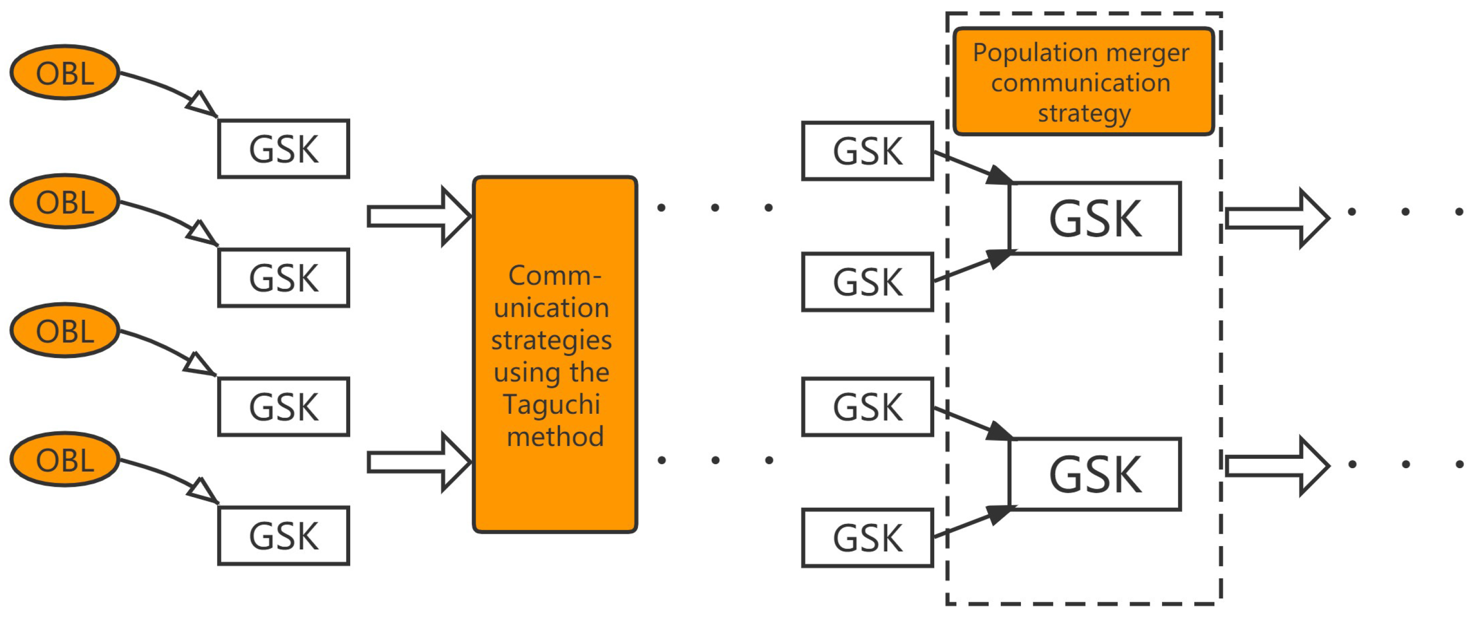
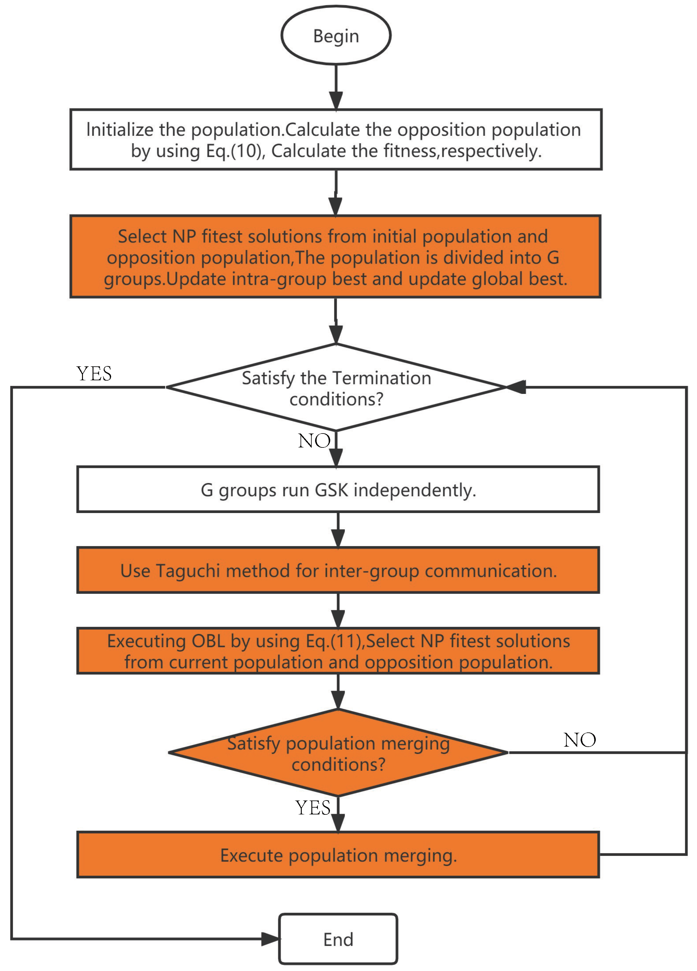
In this paper, several different approaches are considered for integration with GSK and Figure 1 illustrates the process. In POGSK, the initial population is divided into four subpopulations after OBL optimization and the four subpopulations independently conduct GSK and communicate with each generation according to the Taguchi method. After updating the current population, the OBL operation is performed. The pseudocode for POGSK is shown in Algorithm 4. Moreover, in order to demonstrate the POGSK process more visually, Figure 2 shows its main processes.
| Algorithm 4: POGSK pseudo-code |
 |
3.3. Apply the POGSK to Solve the Resource-Scheduling Problem in IoV
In order to reasonably allocate the resources of RSUs in IoV and enhance the QoS, this paper proposes the following mathematical model. Assume that there are multiple vehicles on the road and a total of n tasks are submitted simultaneously and each task contains four attributes: (1) the size of the task; (2) deadlines for tasks; (3) type and quantity of resources required; (4) the transfer time of the submitted work. The n tasks are represented as follows [36]:
Suppose that there are m processing nodes in the current scenario. Each processing unit contains two attributes: (1) type and quantity of resources owned by the processing unit and (2) the processing capacity of the processing unit. The m processing nodes are represented as follows [36]:
- Service delayIn order to provide users with faster services, service latency should be as short as possible. A processing node can handle multiple tasks simultaneously, with different processing capabilities for each node. Then, the processing time of a task on the processing node is [36]where represents the size of the task and represents the processing capability of the processing node . Then, the time required for a processing node to complete all the tasks assigned to it iswhere C(i,j) is a binary value and indicates whether task is assigned to node , denoted asThe sum of the processing delays of all nodes is
- Resource utilizationAccording to research, the energy consumption of the server in the idle state can account for more than 60% of the full load operation [42], which leads to a large amount of energy wasted on the idle server. So we want the roadside unit to be as resource-efficient as possible. The service request in the IoV requires the support of four kinds of computer resources, namely CPU, memory, disk and bandwidth. We need to pay attention to all four sources. Then, the total resource utilization iswhere CR(i,k) represents the number of required by , PR(j,k) represents the number of owned by and is a binary value indicating whether is turned on or not (k = 1,2,3,4 represents four resources).
- Load balancingThe service request in the IoV has different demands on different resources; it is easy to cause the load of different types of resources to be unbalanced. A valuable load-balancing technique in cloud computing can enhance the accuracy and efficiency of cloud computing performance [43]. So we want the processing unit to be as load-balanced as possible. Then, the utilization of in iswhere C(i,j) is calculated using Equation (16). The mean of resource utilization of isThe variance of resource utilization of isThe average resource utilization variance for all processing units iswhere is calculated by Equation (19) and z represents the number of processing units opened.
- SecurityIn the IoV, tasks must be completed on schedule to ensure safety, as service requests are made at high speeds. In real scenarios, the network latency and security of the task is important [6,44]. Task deadlines will be sent with task submissions and we want as many tasks as possible to be completed on time. Then, the actual time required to complete the task iswhere is calculated with Equation (14) and TL(i,j) represents the transmission buffer time from to . Then, whether the task is completed on time is expressed as a binary value:where indicates the deadtime of , which is uploaded when the task is submitted. Then, we express the degree of security as the successful execution rate of the task.
Considering the above four objectives, we propose the following fitness function:
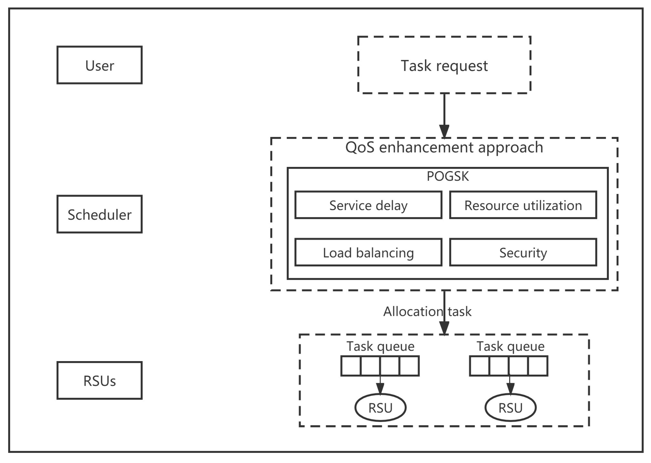
For processing unit , the number of various resources required by all the tasks running on it is not permitted to exceed the number of resources owned by the unit. The workflow is shown in Figure 3. The constraint conditions are:
4. Results
4.1. Simulation Results on CEC2017
Single objective optimization algorithms are the basis of the complex optimization algorithm. It is considered effective to test with some classical mathematical functions. CEC2017 contains 30 benchmark functions to test the optimization ability of the algorithm. The F2 function was abandoned because of the dimension-setting problem. F1 and F3 are Unimodal Functions, F4–F10 are Simple Multimodal Functions, F11–F20 are Hybrid Functions, F21–F30 are Composition Functions. Set error = () as the objective function, where is the actual value of the ith test function and is the minimum value of the ith test function. The optimization goal is to make the error as small as possible. Values of error and standard deviations less than are considered as zero [35].
In this paper, POGSK is compared with the original algorithm GSK, PSO, DE and GWO. The Taguchi strategy in POGSK results in additional fitness function calls in each population generation. So for the sake of fairness, in this paper, the termination condition of the algorithm is set to the maximum number of function evaluations (NEFS) which is set to 10,000*problem_size. For example, the NEFS in a test with 30 variables is 300,000 times. The population size is set to 100 and the range of all test function solutions is set to [−100, 100]. Conduct 31 independent experiments each time to avoid special circumstances. The best results are marked in bold for all problems. The basic parameter settings of each algorithm are shown in Table 3.
Table 4 shows experimental results of POGSK, GSK and DE over 31 independent runs on 29 test functions of 10 variables under CEC2017. Table 5 shows the experimental results of POGSK, GWO and PSO. Compared with the original algorithm GSK, POGSK obtains excellent results in 26 test functions, five of which reach the minimum value of the test function. In contrast to DE, POGSK obtains excellent results on 23 functions. In contrast to GWO, POGSK obtains excellent results on 25 functions. In contrast to PSO, POGSK obtains excellent results on 25 functions. In addition, it is worth noting that POGSK obtained 9 times better results on functions 21–30. This shows that it has excellent search ability on Composition Functions.
Table 6 shows the experimental results of POGSK, GSK and DE over 31 independent runs on 29 test functions of 30 variables under CEC2017. Table 7 shows the experimental results of POGSK, GWO and PSO. Compared with the original algorithm GSK, POGSK obtains excellent results in 20 test functions, five of which reach the minimum value of the test function. In contrast to DE, POGSK obtains excellent results on 26 functions. Compared with GWO, POGSK obtains excellent results on 28 functions. In contrast to PSO, POGSK obtains excellent results on 25 functions. Furthermore, it is worth noting that POGSK obtained 7 times better results on functions 21–30. This again validates its excellent search ability on combinatorial functions.
To demonstrate the algorithm performance of each CEC2017 test problem for multiple numbers of objective function evaluation allowances, we conducted further experiments setting the algorithm termination conditions to 0.1*maximum NFES, 0.3*maximum NFES and 0.5*maximum NFES. Continue using the basic parameters of each algorithm shown in Table 3 without change. Table 8 shows experimental results of POGSK, GSK and PSO over 31 independent runs on 10 variables for multiple numbers of objective function evaluation. Table 9 shows experimental results of POGSK, GWO and DE. For presentation purposes, only the mean fitness values for 31 independent runs of the algorithm are shown in Table 8 and Table 9. It can be observed that in comparison with the 1*max NFES termination condition, POGSK still shows a strong optimization performance when NFES is reduced. It is worth noting that POGSK shows a slight decrease in optimization performance compared to the PSO algorithm. In particular, when NFES = 0.1*Max NFES, POGSK outperforms PSO for only 18 functions. We believe this performance is reasonable because the optimization capability of the POGSK algorithm is not fully utilized when NFES is reduced.
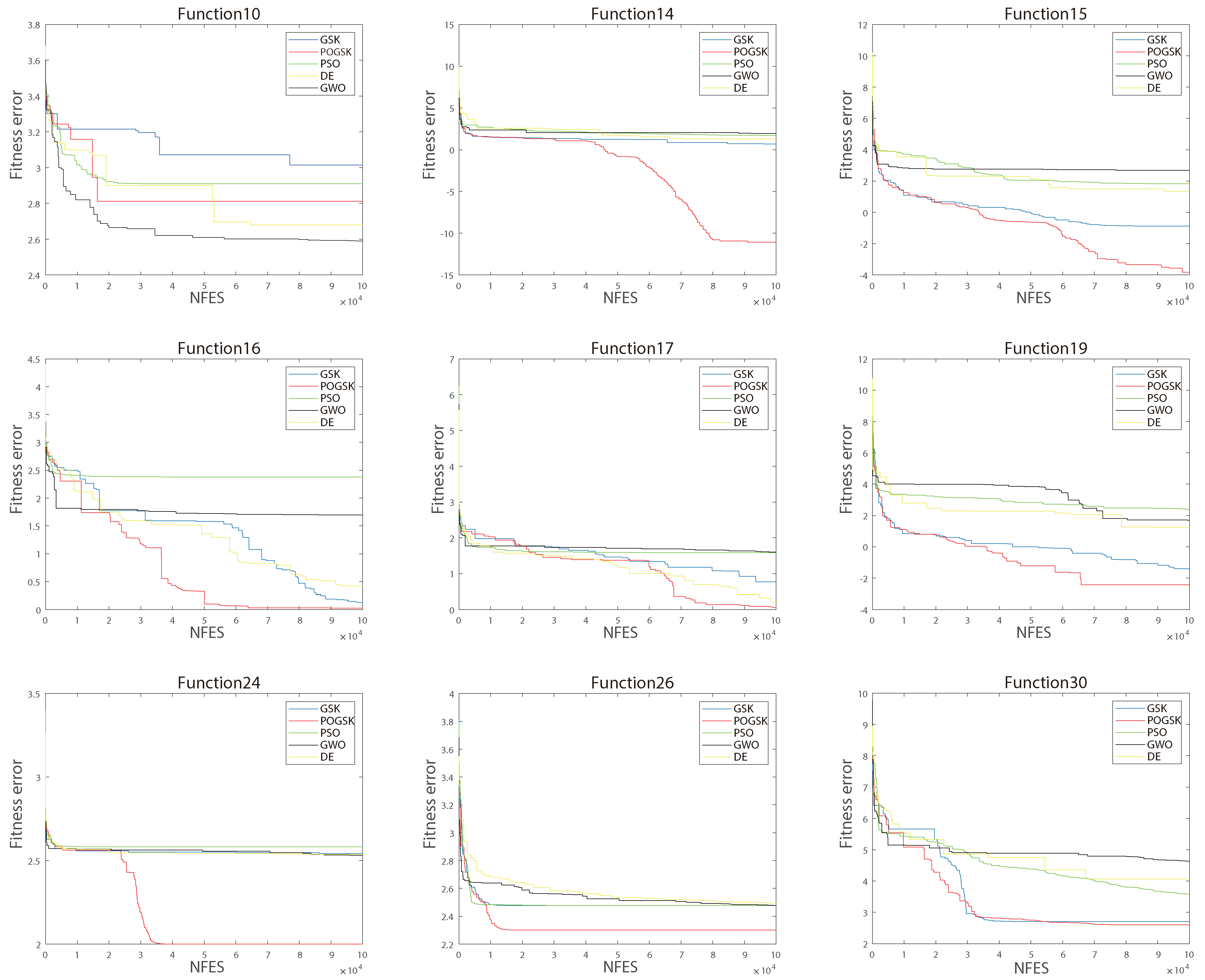
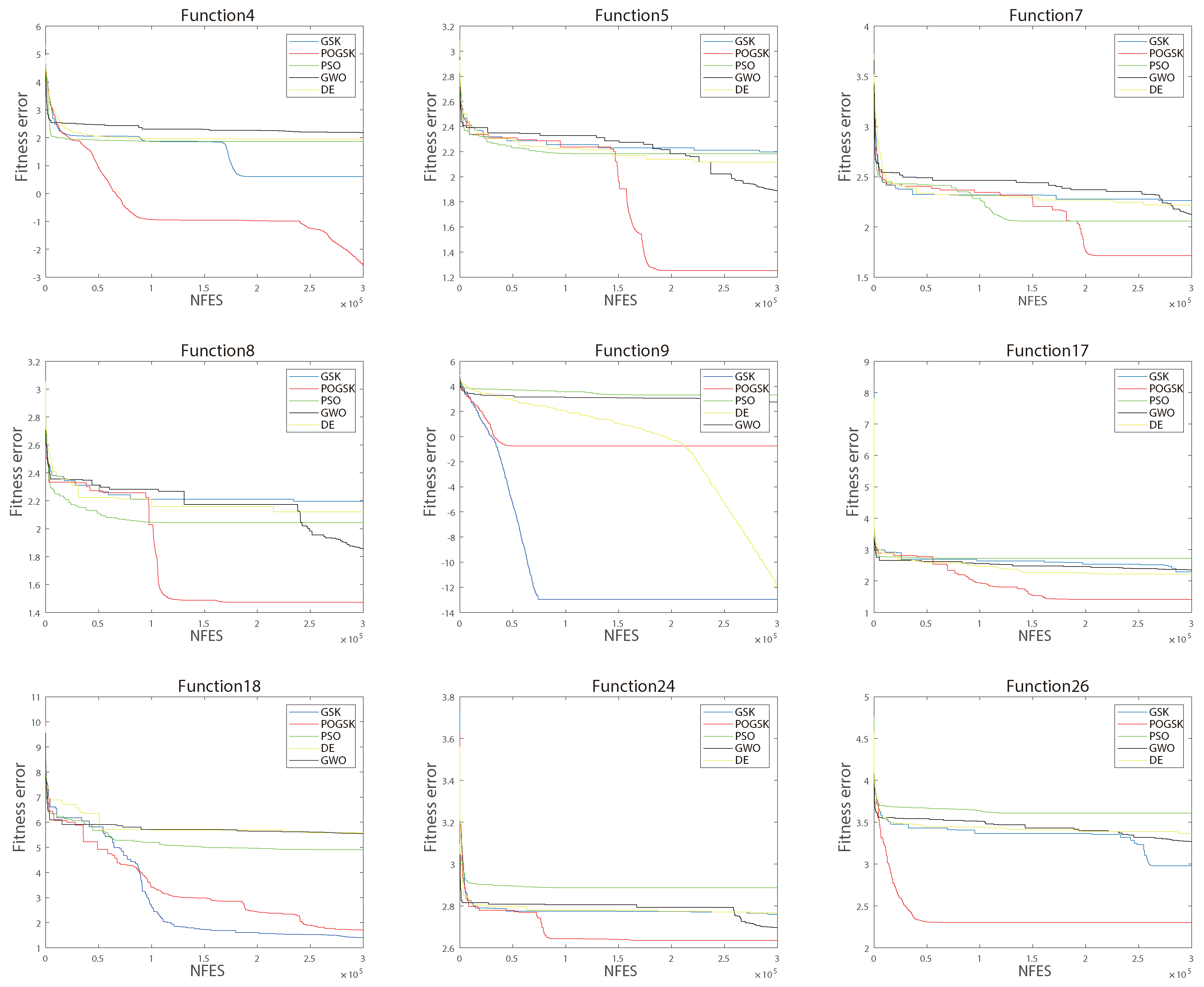
To better visualize the performance of POGSK, the convergence curves of the nine benchmark functions on 10 variables are shown in Figure 4 and the convergence curves of the nine benchmark functions on 30 variables are shown in Figure 5. The convergence curves of POGSK on functions 1–10 of 10 variables are not shown much because unimodal functions and simple multimodal functions are too simple to distinguish the search capability in the case of a few variables. We can see that in the middle and late stages of the algorithm, POGSK shows its powerful search ability to effectively avoid local optima. This reflects the fact that the addition of the OBL strategy and parallel strategy significantly enhances the search capability of the original algorithm. Through the above experimental comparison, it can be determined that POGSK has better capability in the CEC2017 test suite compared with GSK, PSO, DE and GWO.
4.2. Simulation Results on Resource-Scheduling Problems
In this paper, we used the fitness function proposed in Section 3.3 to test the optimized performance of POGSK in real scenarios. We consider the construction of an edge processing system consisting of ten processing units. The size of the tasks to be processed is a random distribution in the interval (0, 5] × instructions. The maximum evaluation times were set as 300,000 times and the population size as 100. In order to avoid exceeding the constraint, the constraint test is carried out when the solution of the algorithm enters the fitness function. Specific constraint testing steps are as follows:
1. Each individual is represented as = {, , …, }, the assignment list {, , …, } is obtained by rounding each dimension of the individual. = b indicates that task i is assigned to node b. All nodes are traversed to find idle nodes and all nodes whose resource utilization is lower than 50%. The idle queues F and low resource utilization queues L are established, respectively. The node is traversed and the over-allocated node is found. Queue is established for the tasks on this node.
2. The tasks in queue are redistributed to the nodes in queue L or to F if L is empty. After each redistribution, the current node is checked to see if it is over-allocated. If not, the current operation is stopped and the process returns to step 3 until all nodes have been traversed. Based on the above results, the individuals need to be adjusted. For example, = 2.1 and = 2. After the constraint test, is adjusted to 6, then is updated randomly in the range [5.6, 6.4].
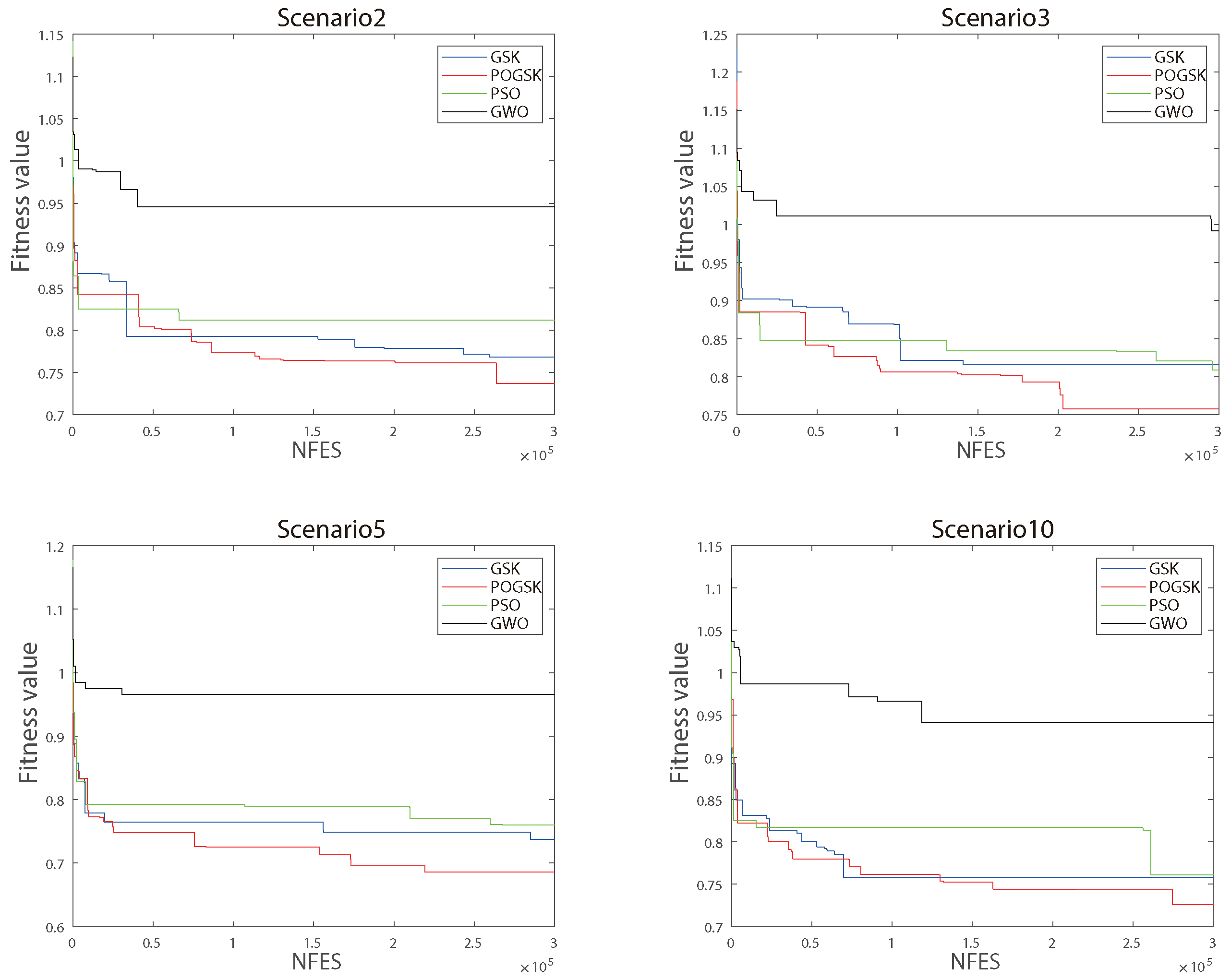
In this paper, we randomly generated 11 independent scenarios which submitted 30 tasks to the processing unit simultaneously. The best results are marked in bold for all scenarios. Table 10 shows other experimental parameters. These experimental parameters control the scene setting in the experiment. Each experiment was independently run 20 times. Table 11 shows the experimental performance of POGSK with GSK, GWO and PSO. You can see that out of the 11 experiments, POGSK won nine times. POGSK achieved excellent results in 9 scenarios compared to GSK. Compared with PSO, POGSK achieved excellent results in 9 scenarios. Compared with GWO, excellent results were obtained in 11 scenarios. This is due to the use of the parallel strategy and the OBL strategy. The Taguchi communication strategy allows the original GSK to effectively avoid falling into a local optimum. The population-merging communication strategy allows POGSK to not weaken algorithm performance due to the reduction in the number of individuals in the subpopulation. The use of the OBL strategy corrects the direction of convergence of the algorithm and increases the speed of convergence.
Figure 6 shows the fitness function value as the number of test function call changes. We can still see that POGSK performs well in avoiding local optimality. It shows that POGSK also performs well in constrained realistic optimization problems.
5. Conclusions
In this paper, the POGSK algorithm is proposed to solve the resource-scheduling problem in the IoV. Based on the original algorithm, POGSK uses OBL and parallel strategy. The information exchange of subpopulations uses the Taguchi strategy and the population-merger strategy. By testing with the original algorithm and some classical algorithms on CEC2017, it is shown that the new algorithm has stronger searching ability. Then, we applied POGSK to the resource-scheduling problem and carried out the simulation test, which also showed better results.
In the future, we can continue to improve the inter-group communication strategy and enhance the search capability of the algorithm. We can also study the application of POGSK in multi-objective problems, engineering optimization problems and binary optimization problems. We believe the new algorithm can also achieve better results.
Author Contributions
Conceptualization, J.-S.P.; methodology, J.-S.P. and L.-F.L.; software, J.-S.P. and L.-F.L.; validation, L.-F.L. and S.-C.C.; investigation, L.-F.L.; resources, J.-S.P. and P.-C.S.; data curation, G.-G.L. and P.-C.S.; writing—original draft preparation, L.-F.L.; writing—review and editing, J.-S.P. and P.-C.S.; supervision, G.-G.L.; project administration, S.-C.C. All authors have read and agreed to the published version of the manuscript.
Funding
This research received no external funding.
Data Availability Statement
The datasets generated for this study are available on request to the corresponding author.
Conflicts of Interest
The authors declare no conflict of interest.
References
- Wang, H.; Wang, W.; Cui, Z.; Zhou, X.; Zhao, J.; Li, Y. A new dynamic firefly algorithm for demand estimation of water resources. Inf. Sci. 2018, 438, 95–106. [Google Scholar] [CrossRef]
- Song, B.; Wang, Z.; Zou, L. An improved PSO algorithm for smooth path planning of mobile robots using continuous high-degree Bezier curve. Appl. Soft Comput. 2021, 100, 106960. [Google Scholar] [CrossRef]
- Chai, Q.w.; Chu, S.C.; Pan, J.S.; Hu, P.; Zheng, W.M. A parallel WOA with two communication strategies applied in DV-Hop localization method. EURASIP J. Wirel. Commun. Netw. 2020, 2020, 50. [Google Scholar] [CrossRef]
- Wu, J.; Xu, M.; Liu, F.F.; Huang, M.; Ma, L.; Lu, Z.M. Solar Wireless Sensor Network Routing Algorithm Based on Multi-Objective Particle Swarm Optimization. J. Inf. Hiding Multim. Signal Process. 2021, 12, 1–11. [Google Scholar]
- Deng, W.; Xu, J.; Song, Y.; Zhao, H. Differential evolution algorithm with wavelet basis function and optimal mutation strategy for complex optimization problem. Appl. Soft Comput. 2021, 100, 106724. [Google Scholar] [CrossRef]
- Farid, M.; Latip, R.; Hussin, M.; Hamid, N.A.W.A. Scheduling scientific workflow using multi-objective algorithm with fuzzy resource utilization in multi-cloud environment. IEEE Access 2020, 8, 24309–24322. [Google Scholar] [CrossRef]
- Mohamed, A.W.; Hadi, A.A.; Mohamed, A.K. Gaining–sharing knowledge based algorithm for solving optimization problems: A novel nature-inspired algorithm. Int. J. Mach. Learn. Cybern. 2020, 11, 1501–1529. [Google Scholar] [CrossRef]
- Eberhart, R.; Kennedy, J. A new optimizer using particle swarm theory. In Proceedings of the MHS’95, Sixth International Symposium on Micro Machine and Human Science, Nagoya, Japan, 4–6 October 1995; pp. 39–43. [Google Scholar]
- Song, P.C.; Chu, S.C.; Pan, J.S.; Yang, H. Simplified Phasmatodea population evolution algorithm for optimization. Complex Intell. Syst. 2022, 8, 2749–2767. [Google Scholar] [CrossRef]
- Pan, J.S.; Zhang, L.G.; Wang, R.B.; Snášel, V.; Chu, S.C. Gannet optimization algorithm: A new metaheuristic algorithm for solving engineering optimization problems. Math. Comput. Simul. 2022, 202, 343–373. [Google Scholar] [CrossRef]
- Mirjalili, S.; Mirjalili, S.M.; Lewis, A. Grey wolf optimizer. Adv. Eng. Softw. 2014, 69, 46–61. [Google Scholar] [CrossRef] [Green Version]
- Chu, S.C.; Tsai, P.W.; Pan, J.S. Cat swarm optimization. In Proceedings of the PRICAI 2006: Trends in Artificial Intelligence: 9th Pacific Rim International Conference on Artificial Intelligence, Guilin, China, 7–11 August 2006; Proceedings 9. Springer: Berlin/Heidelberg, Germany; 2006, pp. 854–858. [Google Scholar]
- Holland, J.H. Genetic algorithms. Sci. Am. 1992, 267, 66–73. [Google Scholar] [CrossRef]
- Storn, R.; Price, K. Differential evolution-a simple and efficient heuristic for global optimization over continuous spaces. J. Glob. Optim. 1997, 11, 341. [Google Scholar] [CrossRef]
- Han, K.H.; Kim, J.H. Quantum-inspired evolutionary algorithm for a class of combinatorial optimization. IEEE Trans. Evol. Comput. 2002, 6, 580–593. [Google Scholar] [CrossRef] [Green Version]
- Hashim, F.A.; Hussain, K.; Houssein, E.H.; Mabrouk, M.S.; Al-Atabany, W. Archimedes optimization algorithm: A new metaheuristic algorithm for solving optimization problems. Appl. Intell. 2021, 51, 1531–1551. [Google Scholar] [CrossRef]
- Kirkpatrick, S.; Gelatt, C.D., Jr.; Vecchi, M.P. Optimization by simulated annealing. Science 1983, 220, 671–680. [Google Scholar] [CrossRef]
- Mirjalili, S. SCA: A sine cosine algorithm for solving optimization problems. Knowl.-Based Syst. 2016, 96, 120–133. [Google Scholar] [CrossRef]
- Rao, R.V.; Savsani, V.J.; Vakharia, D. Teaching–learning-based optimization: A novel method for constrained mechanical design optimization problems. Comput.-Aided Des. 2011, 43, 303–315. [Google Scholar] [CrossRef]
- Mohamed, A.W.; Abutarboush, H.F.; Hadi, A.A.; Mohamed, A.K. Gaining–sharing knowledge based algorithm with adaptive parameters for engineering optimization. IEEE Access 2021, 9, 65934–65946. [Google Scholar] [CrossRef]
- Chu, S.C.; Roddick, J.F.; Pan, J.S. A parallel particle swarm optimization algorithm with communication strategies. J. Inf. Sci. Eng 2005, 21, 809–818. [Google Scholar]
- Harada, T.; Alba, E. Parallel genetic algorithms: A useful survey. ACM Comput. Surv. CSUR 2020, 53, 1–39. [Google Scholar] [CrossRef]
- Cai, D.; Lei, X. A New Evolutionary Algorithm Based on Uniform and Contraction for Many-objective Optimization. J. Netw. Intell. 2017, 2, 171–185. [Google Scholar]
- Tsai, P.W.; Pan, J.S.; Chen, S.M.; Liao, B.Y. Enhanced parallel cat swarm optimization based on the Taguchi method. Expert Syst. Appl. 2012, 39, 6309–6319. [Google Scholar] [CrossRef]
- Tsai, J.T.; Liu, T.K.; Chou, J.H. Hybrid Taguchi-genetic algorithm for global numerical optimization. IEEE Trans. Evol. Comput. 2004, 8, 365–377. [Google Scholar] [CrossRef]
- Jiang, S.J.; Chu, S.C.; Zou, F.M.; Shan, J.; Zheng, S.G.; Pan, J.S. A parallel Archimedes optimization algorithm based on Taguchi method for application in the control of variable pitch wind turbine. Math. Comput. Simul. 2023, 203, 306–327. [Google Scholar] [CrossRef]
- Mahdavi, S.; Rahnamayan, S.; Deb, K. Opposition based learning: A literature review. Swarm Evol. Comput. 2018, 39, 1–23. [Google Scholar] [CrossRef]
- Yu, X.; Xu, W.; Li, C. Opposition-based learning grey wolf optimizer for global optimization. Knowl.-Based Syst. 2021, 226, 107139. [Google Scholar] [CrossRef]
- Dhargupta, S.; Ghosh, M.; Mirjalili, S.; Sarkar, R. Selective opposition based grey wolf optimization. Expert Syst. Appl. 2020, 151, 113389. [Google Scholar] [CrossRef]
- Rahnamayan, S.; Tizhoosh, H.R.; Salama, M.M. Opposition-based differential evolution. IEEE Trans. Evol. Comput. 2008, 12, 64–79. [Google Scholar] [CrossRef] [Green Version]
- Deng, W.; Shang, S.; Cai, X.; Zhao, H.; Song, Y.; Xu, J. An improved differential evolution algorithm and its application in optimization problem. Soft Comput. 2021, 25, 5277–5298. [Google Scholar] [CrossRef]
- Wang, H.; Wu, Z.; Rahnamayan, S.; Liu, Y.; Ventresca, M. Enhancing particle swarm optimization using generalized opposition-based learning. Inf. Sci. 2011, 181, 4699–4714. [Google Scholar] [CrossRef]
- Ewees, A.A.; Abd Elaziz, M.; Houssein, E.H. Improved grasshopper optimization algorithm using opposition-based learning. Expert Syst. Appl. 2018, 112, 156–172. [Google Scholar] [CrossRef]
- Mohamed, A.W.; Hadi, A.A.; Mohamed, A.K.; Awad, N.H. Evaluating the performance of adaptive gainingsharing knowledge based algorithm on CEC 2020 benchmark problems. In Proceedings of the 2020 IEEE Congress on Evolutionary Computation (CEC), Glasgow, UK, 19–24 July 2020; pp. 1–8. [Google Scholar]
- Awad, N.; Ali, M.; Liang, J.; Qu, B.; Suganthan, P. Problem Definitions and Evaluation Criteria for The CEC 2017 Special Session and Competition on Single Objective Real-Parameter Numerical Optimization; Technical Report; Nanyang Technological University: Singapore, 2016. [Google Scholar]
- Cao, B.; Zhang, J.; Liu, X.; Sun, Z.; Cao, W.; Nowak, R.M.; Lv, Z. Edge–Cloud Resource Scheduling in Space–Air–Ground-Integrated Networks for Internet of Vehicles. IEEE Internet Things J. 2022, 9, 5765–5772. [Google Scholar] [CrossRef]
- Ðurasević, M.; Jakobović, D. Heuristic and metaheuristic methods for the parallel unrelated machines scheduling problem: A survey. Artif. Intell. Rev. 2022, 56, 3181–3289. [Google Scholar] [CrossRef]
- Singh, S.; Chana, I. QoS-aware autonomic resource management in cloud computing: A systematic review. ACM Comput. Surv. CSUR 2015, 48, 1–46. [Google Scholar] [CrossRef]
- Yao, J. Research on Optimization Algorithm for Resource Allocation of Heterogeneous Car Networking Engineering Cloud System Based on Big Data. Math. Probl. Eng. 2022, 2022, 1079750. [Google Scholar] [CrossRef]
- Wang, Q.; Guo, S.; Liu, J.; Yang, Y. Energy-efficient computation offloading and resource allocation for delay-sensitive mobile edge computing. Sustain. Comput. Inform. Syst. 2019, 21, 154–164. [Google Scholar] [CrossRef]
- Filip, I.D.; Pop, F.; Serbanescu, C.; Choi, C. Microservices scheduling model over heterogeneous cloud-edge environments as support for IoT applications. IEEE Internet Things J. 2018, 5, 2672–2681. [Google Scholar] [CrossRef]
- Guo, M.; Li, L.; Guan, Q. Energy-efficient and delay-guaranteed workload allocation in IoT-edge-cloud computing systems. IEEE Access 2019, 7, 78685–78697. [Google Scholar] [CrossRef]
- Ullah, A.; Nawi, N.M.; Ouhame, S. Recent advancement in VM task allocation system for cloud computing: Review from 2015 to2021. Artif. Intell. Rev. 2022, 55, 2529–2573. [Google Scholar] [CrossRef]
- Cao, B.; Sun, Z.; Zhang, J.; Gu, Y. Resource allocation in 5G IoV architecture based on SDN and fog-cloud computing. IEEE Trans. Intell. Transp. Syst. 2021, 22, 3832–3840. [Google Scholar] [CrossRef]
Figure 1.
The approaches of POGSK.

Figure 2.
The flowchart of POGSK.

Figure 3.
Scheduling model.

Figure 4.
Convergence curves of 9 functions on 10 variables.

Figure 5.
Convergence curves of 9 functions on 30 variables.

Figure 6.
Convergence curves of four situations.


Table 1.
The position of the candidate individuals.
| Position | Dimension | |||||||
|---|---|---|---|---|---|---|---|---|
| 1 | 2 | 3 | 4 | 5 | 6 | 7 | Fitness Value | |
| 0 | 1 | 1 | 0 | 0 | 1 | 0 | 3 | |
| 1 | 0 | 0 | 1 | 1 | 0 | 1 | 4 | |
Table 2.
The Taguchi method is used to produce better individuals.
| Experiment Number | Dimension | |||||||
|---|---|---|---|---|---|---|---|---|
| 1 | 2 | 3 | 4 | 5 | 6 | 7 | Fitness Value | |
| 1 | 0 | 1 | 1 | 0 | 0 | 1 | 0 | 3 |
| 2 | 0 | 1 | 1 | 1 | 1 | 0 | 1 | 5 |
| 3 | 0 | 0 | 0 | 0 | 0 | 0 | 1 | 1 |
| 4 | 0 | 0 | 0 | 1 | 1 | 1 | 0 | 3 |
| 5 | 1 | 1 | 0 | 0 | 1 | 1 | 1 | 5 |
| 6 | 1 | 1 | 0 | 1 | 0 | 0 | 0 | 3 |
| 7 | 1 | 0 | 1 | 0 | 1 | 0 | 0 | 3 |
| 8 | 1 | 0 | 1 | 1 | 0 | 1 | 1 | 5 |
| cumulative fitness value | 12 | 16 | 16 | 12 | 12 | 16 | 12 | - |
| cumulative fitness value | 16 | 12 | 12 | 16 | 16 | 12 | 16 | - |
| Selected dimension source | - | |||||||
| Position of the new individual | 0 | 0 | 0 | 0 | 0 | 0 | 0 | 0 |
Table 3.
Parameter settings of each algorithm.
| Algorithms | Parameters Settings |
|---|---|
| POGSK | G = 4, R = 0.5, L = 1, r = 0.1, = 0.5, = 0.9, K = 1 |
| GSK | = 0.5, = 0.9, K = 1 |
| PSO | = 6, = −6, wMax = 0.9, wMin = 0.2, c1 = c2 = 2 |
| DE | = 0.2, = 0.8, pCR = 0.2 |
| GWO | = 2 (linearly decreased over iterations) |
Table 4.
Experimental results of POGSK, GSK and DE over 31 independent runs on 29 test functions of 10 variables under CEC2017.
Table 4.
Experimental results of POGSK, GSK and DE over 31 independent runs on 29 test functions of 10 variables under CEC2017.
| Function | POGSK | GSK | DE | |||
|---|---|---|---|---|---|---|
| Mean | Std | Mean | Std | Mean | Std | |
| 1 | 0 | 0 | 0 | 0 | 1243.046 | 917.0439 |
| 3 | 0 | 0 | 0 | 0 | 1521.115 | 622.8467 |
| 4 | 0 | 0 | 0 | 0 | 6.037244 | 0.307901 |
| 5 | 17.48551 | 4.653999 | 20.50791 | 3.041351 | 9.710514 | 1.981759 |
| 6 | 0 | 0 | 0 | 0 | 0 | 0 |
| 7 | 29.31611 | 4.914915 | 30.33268 | 3.706216 | 20.85221 | 1.880978 |
| 8 | 17.00134 | 4.4744 | 19.45566 | 3.871004 | 9.794002 | 1.752965 |
| 9 | 0 | 0 | 0 | 0 | 0 | 0 |
| 10 | 930.7502 | 187.4053 | 1022.488 | 101.7212 | 492.0772 | 107.547 |
| 11 | 0.288859 | 0.459088 | 0 | 0 | 3.254768 | 0.650172 |
| 12 | 102.7016 | 87.50214 | 80.9387 | 62.50609 | 162,272.8 | 84,043.21 |
| 13 | 4.39938 | 2.902828 | 6.489874 | 1.622716 | 1247.31 | 1044.067 |
| 14 | 0.87396 | 0.883004 | 5.982104 | 2.986793 | 26.23902 | 20.65982 |
| 15 | 0.15139 | 0.27689 | 0.313974 | 0.29665 | 28.17154 | 24.51716 |
| 16 | 0.99709 | 2.036369 | 2.917096 | 4.299084 | 3.314234 | 1.910263 |
| 17 | 1.82295 | 3.702029 | 9.250251 | 6.796455 | 1.89604 | 0.899154 |
| 18 | 1.67142 | 4.206737 | 1.673515 | 5.02943 | 967.1823 | 585.524 |
| 19 | 0.0497 | 0.056623 | 0.104905 | 0.114554 | 27.60279 | 33.09174 |
| 20 | 0.446523 | 0.312835 | 0.414759 | 0.211807 | 0 | 0 |
| 21 | 176.3012 | 57.57345 | 193.0073 | 51.14463 | 161.4336 | 36.74808 |
| 22 | 95.8506 | 16.53658 | 100.3894 | 0.814027 | 97.40993 | 9.366758 |
| 23 | 306.122 | 2.840924 | 317.7665 | 3.307184 | 312.0515 | 2.093624 |
| 24 | 306.697 | 81.28064 | 341.4343 | 21.0113 | 316.2438 | 39.04365 |
| 25 | 399.464 | 8.161678 | 427.1743 | 21.27511 | 410.4391 | 9.406591 |
| 26 | 296.774 | 17.96053 | 300 | 2.99E−13 | 300.5042 | 52.62727 |
| 27 | 389.217 | 0.239349 | 389.5044 | 0.052422 | 389.5575 | 0.2579 |
| 28 | 300 | 2.67E−13 | 303.1151 | 17.34415 | 430.3714 | 69.26502 |
| 29 | 243.926 | 5.174707 | 248.3445 | 5.043812 | 263.9279 | 8.011281 |
| 30 | 445.736 | 38.26841 | 7363.998 | 38,494.24 | 13,511.91 | 7149.584 |
| Win | - | - | 26 | 15 | 23 | 18 |
| Lose | - | - | 3 | 14 | 6 | 11 |
Table 5.
Experimental results of POGSK, PSO and GWO over 31 independent runs on 29 test functions of 10 variables under CEC2017.
Table 5.
Experimental results of POGSK, PSO and GWO over 31 independent runs on 29 test functions of 10 variables under CEC2017.
| Function | POGSK | GWO | PSO | |||
|---|---|---|---|---|---|---|
| Mean | Std | Mean | Std | Mean | Std | |
| 1 | 0 | 0 | 4,497,091 | 11,601,735 | 1159.397 | 1605.775 |
| 3 | 0 | 0 | 259.1001 | 389.8524 | 0 | 0 |
| 4 | 0 | 0 | 9.201156 | 5.959095 | 3.91603 | 12.5333 |
| 5 | 17.48551 | 4.653999 | 13.25237 | 7.436721 | 28.50068 | 9.743601 |
| 6 | 0 | 0 | 0.464612 | 0.881753 | 4.077067 | 3.713828 |
| 7 | 29.31611 | 4.914915 | 26.10298 | 8.270842 | 21.02474 | 6.645744 |
| 8 | 17.00134 | 4.4744 | 11.49256 | 4.369928 | 15.46999 | 6.8877 |
| 9 | 0 | 0 | 3.344128 | 8.094291 | 0 | 0 |
| 10 | 930.7502 | 187.4053 | 455.7428 | 250.51 | 793.989 | 304.649 |
| 11 | 0.288859 | 0.459088 | 19.59614 | 25.7201 | 23.76794 | 11.81411 |
| 12 | 102.7016 | 87.50214 | 480,552.9 | 684,130.6 | 12,243.2 | 11,168.19 |
| 13 | 4.39938 | 2.902828 | 8697.586 | 4995.097 | 7018.655 | 5919.406 |
| 14 | 0.87396 | 0.883004 | 1108.531 | 1650.036 | 78.09055 | 101.3466 |
| 15 | 0.15139 | 0.27689 | 1291.43 | 1574.817 | 238.5524 | 322.1582 |
| 16 | 0.99709 | 2.036369 | 77.88443 | 69.76017 | 212.4675 | 118.4518 |
| 17 | 1.82295 | 3.702029 | 44.01848 | 19.88944 | 43.69786 | 25.65489 |
| 18 | 1.67142 | 4.206737 | 28,538.6 | 14,703.86 | 8380.526 | 5920.313 |
| 19 | 0.0497 | 0.056623 | 4300.029 | 5439.223 | 619.0984 | 767.2034 |
| 20 | 0.446523 | 0.312835 | 51.83766 | 39.56463 | 63.11953 | 46.19121 |
| 21 | 176.3012 | 57.57345 | 208.0848 | 19.82006 | 173.3363 | 63.70194 |
| 22 | 95.8506 | 16.53658 | 103.3866 | 17.3914 | 102.3462 | 0.964004 |
| 23 | 306.122 | 2.840924 | 315.7259 | 7.263185 | 361.6049 | 72.55207 |
| 24 | 306.697 | 81.28064 | 337.3761 | 43.27372 | 348.4116 | 106.5231 |
| 25 | 399.464 | 8.161678 | 439.6042 | 13.4442 | 425.0482 | 23.00597 |
| 26 | 296.774 | 17.96053 | 355.5426 | 169.6211 | 367.0571 | 174.7731 |
| 27 | 389.217 | 0.239349 | 397.2865 | 17.07097 | 432.788 | 42.47196 |
| 28 | 300 | 2.67E−13 | 537.1552 | 99.1675 | 377.7298 | 48.39093 |
| 29 | 243.926 | 5.174707 | 275.9368 | 34.50598 | 308.0478 | 38.2051 |
| 30 | 445.736 | 38.26841 | 601,218.1 | 684,207.6 | 4893.086 | 3573.952 |
| Win | - | - | 25 | 26 | 25 | 28 |
| Lose | - | - | 4 | 3 | 4 | 1 |
Table 6.
Experimental results of POGSK, GSK and DE over 31 independent runs on 29 test functions of 30 variables under CEC2017.
Table 6.
Experimental results of POGSK, GSK and DE over 31 independent runs on 29 test functions of 30 variables under CEC2017.
| Function | POGSK | GSK | DE | |||
|---|---|---|---|---|---|---|
| Mean | Std | Mean | Std | Mean | Std | |
| 1 | 0 | 0 | 0 | 0 | 565.1619 | 467.5469 |
| 2 | 0.1710225 | 0.951944 | 1.27E−07 | 3.59E−07 | 78,485.43 | 11,969.56 |
| 3 | 2.3896 | 2.00382 | 8.0680906 | 15.72576 | 88.87305 | 1.39142 |
| 4 | 32.70072 | 9.603168 | 157.06186 | 10.58822 | 129.9884 | 9.275313 |
| 5 | 4.78E−05 | 7.06E−05 | 6.48E−07 | 1.44E−06 | 0 | 0 |
| 6 | 110.9293 | 59.25905 | 184.5384 | 10.80525 | 163.7576 | 10.61515 |
| 7 | 31.70902 | 9.949111 | 157.84376 | 8.553038 | 130.7675 | 8.930799 |
| 8 | 1.3961111 | 0.964445 | 0 | 0 | 0 | 0 |
| 9 | 6640.146 | 352.1547 | 6773.1382 | 280.2139 | 5270.445 | 300.3687 |
| 10 | 15.3527 | 8.172784 | 32.010214 | 37.36949 | 110.2576 | 10.49883 |
| 11 | 7473.1514 | 4191.488 | 5872.033 | 3954.488 | 4,064,732 | 1,326,017 |
| 12 | 68.10246 | 33.29562 | 97.603211 | 38.84956 | 146,977.1 | 70,134.12 |
| 13 | 47.58591 | 13.26488 | 56.580342 | 4.594124 | 59,985.92 | 29,927.38 |
| 14 | 32.795131 | 16.27245 | 16.78781 | 10.92508 | 20,442.66 | 11,240.16 |
| 15 | 225.2992 | 208.1208 | 795.64371 | 166.3631 | 588.2006 | 138.6957 |
| 16 | 47.13605 | 16.82453 | 198.98593 | 92.83664 | 162.9097 | 38.25502 |
| 17 | 104.56587 | 64.00951 | 36.67658 | 8.700766 | 424,098.9 | 151,960.3 |
| 18 | 22.242391 | 8.28202 | 10.97738 | 4.416147 | 19,255.23 | 9427.15 |
| 19 | 62.56111 | 50.53387 | 68.739206 | 65.88684 | 173.8984 | 49.83044 |
| 20 | 234.2304 | 20.45764 | 349.17774 | 8.751155 | 332.6374 | 8.650852 |
| 21 | 100.07935 | 0.441787 | 100 | 4.52E−13 | 1202.919 | 888.6275 |
| 22 | 374.781 | 6.959946 | 463.52232 | 59.16068 | 480.7536 | 7.607155 |
| 23 | 444.1957 | 6.710317 | 567.06927 | 29.46917 | 582.855 | 8.472587 |
| 24 | 385.91772 | 1.780967 | 386.92029 | 0.19508 | 387.3266 | 0.082705 |
| 25 | 685.0133 | 500.7473 | 1035.9259 | 330.0292 | 2326.135 | 82.41891 |
| 26 | 496.61134 | 7.400898 | 492.5301 | 7.147451 | 509.6858 | 2.319662 |
| 27 | 303.3373 | 18.54975 | 321.05968 | 43.75981 | 427.0414 | 13.69322 |
| 28 | 460.2316 | 41.83653 | 563.47372 | 111.3137 | 729.1611 | 76.50307 |
| 29 | 2045.674 | 80.2348 | 2080.6714 | 121.1253 | 20,973.93 | 6734.785 |
| Win | - | - | 20 | 12 | 26 | 15 |
| Lose | - | - | 9 | 17 | 3 | 14 |
Table 7.
Experimental results of POGSK, GWO and PSO over 31 independent runs on 29 test functions of 30 variables under CEC2017.
Table 7.
Experimental results of POGSK, GWO and PSO over 31 independent runs on 29 test functions of 30 variables under CEC2017.
| Function | POGSK | GWO | PSO | |||
|---|---|---|---|---|---|---|
| Mean | Std | Mean | Std | Mean | Std | |
| 1 | 0 | 0 | 1.065E+09 | 9.63E+08 | 2399.513 | 3445.498 |
| 3 | 0.1710225 | 0.951944 | 28,199.902 | 10,867.38 | 0.059275 | 0.066189 |
| 4 | 2.3896 | 2.00382 | 160.71215 | 47.20044 | 60.0721 | 28.92923 |
| 5 | 32.70072 | 9.603168 | 78.084404 | 18.62267 | 152.9662 | 25.34413 |
| 6 | 4.78E−05 | 7.06E−05 | 4.5010838 | 2.508565 | 31.18878 | 7.532825 |
| 7 | 110.9293 | 59.25905 | 136.85245 | 23.06388 | 117.7735 | 23.32769 |
| 8 | 31.70902 | 9.949111 | 73.037706 | 18.75822 | 115.3826 | 25.07128 |
| 9 | 1.3961111 | 0.964445 | 524.43328 | 280.1444 | 2084.344 | 424.3998 |
| 10 | 6640.146 | 352.1547 | 2822.749 | 522.9234 | 3384.133 | 730.3928 |
| 11 | 15.3527 | 8.172784 | 296.75347 | 137.9677 | 90.02398 | 17.27491 |
| 12 | 7473.1514 | 4191.488 | 28,314,824 | 40,351,462 | 49,597.69 | 29,308.71 |
| 13 | 68.10246 | 33.29562 | 5,377,176.9 | 23,990,313 | 11,223.13 | 12,434.89 |
| 14 | 47.58591 | 13.26488 | 109,516.46 | 312,614.9 | 7271.957 | 5769.247 |
| 15 | 32.795131 | 16.27245 | 309,301.92 | 786,455 | 6660.235 | 7995.343 |
| 16 | 225.2992 | 208.1208 | 673.1389 | 239.9596 | 1021.81 | 208.1095 |
| 17 | 47.13605 | 16.82453 | 224.34632 | 107.809 | 518.3412 | 162.6259 |
| 18 | 104.56587 | 64.00951 | 449,259.69 | 471,076.9 | 113,207.1 | 84,886.55 |
| 19 | 22.242391 | 8.28202 | 680,051.23 | 1,796,562 | 10,046.08 | 14,864.67 |
| 20 | 62.56111 | 50.53387 | 316.20714 | 113.958 | 425.1631 | 129.9895 |
| 21 | 234.2304 | 20.45764 | 269.79579 | 15.67731 | 324.6484 | 26.97333 |
| 22 | 100.07935 | 0.441787 | 2207.2882 | 1473.069 | 1253.874 | 1862.064 |
| 23 | 374.781 | 6.959946 | 430.27783 | 38.0415 | 708.1221 | 116.4942 |
| 24 | 444.1957 | 6.710317 | 514.80412 | 50.32647 | 778.1768 | 72.14411 |
| 25 | 385.91772 | 1.780967 | 455.40908 | 24.09939 | 379.621 | 6.204345 |
| 26 | 685.0133 | 500.7473 | 1924.7685 | 304.0471 | 3503.61 | 1534.257 |
| 27 | 496.61134 | 7.400898 | 533.23588 | 12.11012 | 494.1057 | 71.15496 |
| 28 | 303.3373 | 18.54975 | 562.25313 | 62.77035 | 371.5156 | 61.83288 |
| 29 | 460.2316 | 41.83653 | 781.81747 | 149.2681 | 917.2247 | 292.7391 |
| 30 | 2045.674 | 80.2348 | 4,740,432.9 | 4,505,133 | 3024.257 | 4562.477 |
| Win | - | - | 28 | 26 | 25 | 26 |
| Lose | - | - | 1 | 3 | 4 | 3 |
Table 8.
Experimental results of POGSK, GSK and PSO over 31 independent runs on 10 variables for multiple numbers of objective function evaluation.
Table 8.
Experimental results of POGSK, GSK and PSO over 31 independent runs on 10 variables for multiple numbers of objective function evaluation.
| Function | POGSK | GSK | PSO | ||||||
|---|---|---|---|---|---|---|---|---|---|
| 0.1*Max | 0.3*Max | 0.5*Max | 0.1*Max | 0.3*Max | 0.5*Max | 0.1*Max | 0.3*Max | 0.5*Max | |
| 1 | 65,168.64 | 0.008729 | 9.00E−08 | 198,621.8 | 0.148295 | 1.24E−07 | 1507.631 | 1841.959 | 1481.528 |
| 3 | 1072.874 | 0.020955 | 1.37E−09 | 1258.366 | 0.150523 | 3.43E−08 | 3.622942 | 1.32E−06 | 0 |
| 4 | 4.46869 | 0.156832 | 0.000642 | 4.782125 | 0.0252 | 1.26E−05 | 6.788089 | 9.600704 | 4.619372 |
| 5 | 35.91597 | 28.17189 | 22.91988 | 35.00533 | 29.01222 | 23.6099 | 31.58184 | 30.49059 | 29.62402 |
| 6 | 0.67712 | 0.000231 | 3.46E−07 | 1.131835 | 0.001475 | 9.12E−06 | 9.346549 | 4.068655 | 5.220518 |
| 7 | 46.40205 | 36.92188 | 34.41898 | 50.00724 | 37.96985 | 34.8906 | 28.87082 | 24.42772 | 23.73282 |
| 8 | 34.3193 | 26.88238 | 22.69993 | 36.83458 | 28.55074 | 26.63988 | 17.84513 | 15.91932 | 14.53922 |
| 9 | 0.335181 | 0 | 0 | 1.190911 | 0 | 0 | 17.39665 | 6.587552 | 6.853679 |
| 10 | 1532.095 | 1315.312 | 1128.588 | 1525.435 | 1311.749 | 1192.912 | 837.2588 | 806.28 | 762.448 |
| 11 | 11.17021 | 5.209862 | 1.532807 | 12.14115 | 5.79704 | 3.51912 | 26.16613 | 28.79452 | 25.05342 |
| 12 | 91,453.6 | 486.7377 | 199.4322 | 164,573.9 | 617.8236 | 179.6806 | 30,604.58 | 11,899.81 | 16,792.79 |
| 13 | 47.41327 | 12.20971 | 8.403044 | 60.55603 | 11.71106 | 9.488802 | 6398.473 | 9347.321 | 6564.624 |
| 14 | 27.46006 | 19.86859 | 11.84031 | 28.9843 | 18.29269 | 15.361 | 1203.128 | 558.986 | 266.1244 |
| 15 | 9.511309 | 2.529362 | 0.612543 | 10.67048 | 2.489827 | 0.667059 | 2532.754 | 1061.556 | 548.5125 |
| 16 | 83.47293 | 19.34939 | 4.684275 | 91.10372 | 36.5609 | 13.88171 | 216.4358 | 208.4391 | 229.0174 |
| 17 | 71.5188 | 30.70673 | 18.47544 | 85.25013 | 44.12263 | 29.57548 | 49.02151 | 50.02125 | 45.54325 |
| 18 | 74.44131 | 14.67361 | 5.338491 | 162.1569 | 15.29351 | 4.686504 | 13,029.71 | 8474.698 | 8372.767 |
| 19 | 6.425225 | 1.749615 | 0.682905 | 7.216083 | 1.944351 | 0.892702 | 3491.462 | 2753.934 | 2199.245 |
| 20 | 68.77453 | 11.38535 | 1.397734 | 81.44863 | 21.28738 | 3.679158 | 97.71285 | 83.91263 | 75.89307 |
| 21 | 188.5297 | 184.346 | 189.9476 | 209.0319 | 202.3022 | 178.1039 | 171.7462 | 178.0085 | 189.2755 |
| 22 | 103.8606 | 100.5495 | 100.2226 | 105.9777 | 102.3459 | 101.2098 | 131.0425 | 96.96854 | 135.8181 |
| 23 | 335.3295 | 325.8999 | 317.8954 | 335.7887 | 327.2087 | 323.999 | 377.3523 | 369.7106 | 371.4575 |
| 24 | 357.042 | 341.9053 | 316.7562 | 361.736 | 347.599 | 348.096 | 330.8915 | 320.122 | 347.5205 |
| 25 | 403.4286 | 409.5803 | 404.0327 | 420.6563 | 426.9033 | 422.8455 | 415.486 | 420.797 | 423.8288 |
| 26 | 302.3367 | 296.7742 | 296.7742 | 301.0423 | 300 | 300 | 395.6739 | 392.4169 | 469.6308 |
| 27 | 391.4686 | 389.2144 | 389.2638 | 391.1973 | 389.4444 | 389.4419 | 446.6022 | 436.6223 | 439.4359 |
| 28 | 383.6587 | 300.0077 | 303.8159 | 432.3408 | 312.2833 | 300 | 405.3951 | 389.2501 | 350.7108 |
| 29 | 310.7228 | 273.0201 | 257.9113 | 311.5873 | 277.9013 | 266.0836 | 319.5175 | 320.2717 | 321.4858 |
| 30 | 11,6124.7 | 735.7863 | 508.8163 | 169,420.9 | 26,998.33 | 474.5937 | 73,193.34 | 14,707.45 | 9126.257 |
| win | - | - | - | 25 | 24 | 23 | 18 | 22 | 24 |
| lose | - | - | - | 4 | 5 | 6 | 11 | 7 | 5 |
Table 9.
Experimental results of POGSK, GWO and DE over 31 independent runs on 10 variables for multiple numbers of objective function evaluation.
Table 9.
Experimental results of POGSK, GWO and DE over 31 independent runs on 10 variables for multiple numbers of objective function evaluation.
| Function | POGSK | GWO | DE | ||||||
|---|---|---|---|---|---|---|---|---|---|
| 0.1*Max | 0.3*Max | 0.5*Max | 0.1*Max | 0.3*Max | 0.5*Max | 0.1*Max | 0.3*Max | 0.5*Max | |
| 1 | 65,168.64 | 0.008729 | 9.00E−08 | 2,346,406 | 1417856 | 9.565626 | 16,135,020 | 20,544.91 | 4898.193 |
| 3 | 1072.874 | 0.020955 | 1.37E−09 | 2051.369 | 948.2263 | 0.752611 | 14,530.99 | 8845.123 | 5727.654 |
| 4 | 4.46869 | 0.156832 | 0.000642 | 22.33487 | 11.35453 | 29.34763 | 12.85429 | 6.929505 | 6.505718 |
| 5 | 35.91597 | 28.17189 | 22.91988 | 18.45571 | 12.63573 | 13.74093 | 30.60479 | 18.81837 | 14.40469 |
| 6 | 0.67712 | 0.000231 | 3.46E−07 | 1.228019 | 0.823463 | 3.763687 | 1.810073 | 0.001324 | 6.07E−07 |
| 7 | 46.40205 | 36.92188 | 34.41898 | 37.21266 | 29.32247 | 506.0761 | 44.70667 | 30.20338 | 25.16062 |
| 8 | 34.3193 | 26.88238 | 22.69993 | 15.91906 | 15.30446 | 21.20127 | 31.77074 | 20.53481 | 14.54278 |
| 9 | 0.335181 | 0 | 0 | 6.672216 | 8.604824 | 522,798.1 | 41.7464 | 0.017794 | 2.17E−07 |
| 10 | 1532.095 | 1315.312 | 1128.588 | 677.9308 | 573.4273 | 11,452.42 | 1210.891 | 851.5756 | 702.4145 |
| 11 | 11.17021 | 5.209862 | 1.532807 | 30.60828 | 31.73361 | 1246.452 | 47.17272 | 8.057127 | 5.097437 |
| 12 | 91,453.6 | 486.7377 | 199.4322 | 1,407,448 | 643,050.9 | 2140.969 | 6,603,038 | 1,351,308 | 594,344.9 |
| 13 | 47.41327 | 12.20971 | 8.403044 | 11065.19 | 12,549.47 | 90.00417 | 16,654.35 | 4276.951 | 1909.666 |
| 14 | 27.46006 | 19.86859 | 11.84031 | 2450.4 | 1269.145 | 52.02613 | 961.5601 | 184.9314 | 110.3554 |
| 15 | 9.511309 | 2.529362 | 0.612543 | 5154.414 | 3513.667 | 25,350.52 | 1426.507 | 236.2673 | 121.9112 |
| 16 | 83.47293 | 19.34939 | 4.684275 | 118.3694 | 120.0137 | 4220.433 | 96.57352 | 22.84995 | 9.823819 |
| 17 | 71.5188 | 30.70673 | 18.47544 | 68.63565 | 61.1111 | 60.51609 | 53.16403 | 29.56227 | 14.18701 |
| 18 | 74.44131 | 14.67361 | 5.338491 | 24,579.32 | 25,987.05 | 201.3137 | 41,806.47 | 6779.277 | 2723.725 |
| 19 | 6.425225 | 1.749615 | 0.682905 | 9683.89 | 7409.389 | 106.6633 | 2030.003 | 296.4361 | 199.3466 |
| 20 | 68.77453 | 11.38535 | 1.397734 | 88.42235 | 71.2303 | 317.6138 | 37.92879 | 4.11068 | 0.002431 |
| 21 | 188.5297 | 184.346 | 189.9476 | 211.797 | 205.8708 | 342.6138 | 209.201 | 179.1673 | 172.5472 |
| 22 | 103.8606 | 100.5495 | 100.2226 | 111.9155 | 108.5442 | 436.9162 | 126.1442 | 102.526 | 101.7367 |
| 23 | 335.3295 | 325.8999 | 317.8954 | 323.4811 | 317.4113 | 369.5282 | 332.2919 | 319.7871 | 316.0538 |
| 24 | 357.042 | 341.9053 | 316.7562 | 354.3611 | 335.1408 | 398.7922 | 361.1658 | 352.334 | 343.8135 |
| 25 | 403.4286 | 409.5803 | 404.0327 | 439.5899 | 433.9101 | 552.888 | 450.7069 | 431.3259 | 420.7792 |
| 26 | 302.3367 | 296.7742 | 296.7742 | 370.8195 | 374.8314 | 275.9333 | 541.4581 | 399.4515 | 350.68 |
| 27 | 391.4686 | 389.2144 | 389.2638 | 396.9011 | 394.4558 | 852,804.2 | 397.4228 | 391.6064 | 390.2805 |
| 28 | 383.6587 | 300.0077 | 303.8159 | 551.6053 | 539.1753 | 3358.777 | 549.7038 | 511.7699 | 488.9492 |
| 29 | 310.7228 | 273.0201 | 257.9113 | 299.4216 | 291.2249 | 3191.632 | 345.5497 | 296.2041 | 280.3842 |
| 30 | 116,124.7 | 735.7863 | 508.8163 | 491,702 | 795,289.2 | 255,507.2 | 285,465.2 | 70,612.38 | 32,384.37 |
| win | - | - | - | 21 | 23 | 26 | 22 | 21 | 21 |
| lose | - | - | - | 8 | 6 | 3 | 7 | 8 | 8 |
Table 10.
Experimental parameter settings.
| Symbols | Descriptions | Values |
|---|---|---|
| Size of the ith task | (0, 5] × instr | |
| Processing capacity of the jth processing unit | [0.5, 2] × instr/ms | |
| CR(i,k) | The number of required by | [0, 5] |
| PR(i,k) | The number of owned by | [5, 25] |
| TL(i,j) | The transmission buffer time from to | [0, 3] ms |
| Deadtime of | + [0, 3] ms |
Table 11.
A total of 30 tasks were assigned to 10 processing unit experiments.
| Scenario | POGSK | GSK | PSO | GWO | ||||
|---|---|---|---|---|---|---|---|---|
| Mean | Std | Mean | Std | Mean | Std | Mean | Std | |
| 1 | 5.718209 | 0.144952 | 5.855939 | 0.135115 | 6.053149 | 0.248256 | 8.991358 | 0.330173 |
| 2 | 6.329143 | 0.340846 | 6.485126 | 0.241881 | 6.265463 | 0.270268 | 9.997938 | 0.317971 |
| 3 | 5.981696 | 0.163071 | 6.003088 | 0.158414 | 6.339609 | 0.287226 | 9.344461 | 0.246512 |
| 4 | 5.212316 | 0.204313 | 5.36799 | 0.227842 | 5.917752 | 0.393545 | 8.974101 | 0.311377 |
| 5 | 5.245472 | 0.162959 | 5.326294 | 0.247776 | 5.428665 | 0.832814 | 9.157856 | 0.251572 |
| 6 | 5.624188 | 0.115448 | 5.789302 | 0.231226 | 6.21364 | 0.559447 | 9.555559 | 0.421648 |
| 7 | 6.661226 | 0.325418 | 6.793765 | 0.249867 | 6.975366 | 0.409818 | 10.00448 | 0.244958 |
| 8 | 5.158754 | 0.278578 | 4.992622 | 0.156462 | 5.53684 | 0.151473 | 8.233507 | 0.457459 |
| 9 | 5.567888 | 0.096427 | 5.70977 | 0.105788 | 5.874641 | 0.139983 | 8.946471 | 0.32081 |
| 10 | 5.828361 | 0.208058 | 5.929272 | 0.293122 | 6.330107 | 0.47567 | 9.343315 | 0.307779 |
| 11 | 5.677546 | 0.008842 | 5.558177 | 0.175736 | 5.274045 | 0.673208 | 9.222462 | 0.412783 |
| Win | - | - | 9 | 6 | 9 | 9 | 11 | 9 |
| Lose | - | - | 2 | 5 | 2 | 2 | 0 | 2 |
Disclaimer/Publisher’s Note: The statements, opinions and data contained in all publications are solely those of the individual author(s) and contributor(s) and not of MDPI and/or the editor(s). MDPI and/or the editor(s) disclaim responsibility for any injury to people or property resulting from any ideas, methods, instructions or products referred to in the content. |
© 2023 by the authors. Licensee MDPI, Basel, Switzerland. This article is an open access article distributed under the terms and conditions of the Creative Commons Attribution (CC BY) license (https://creativecommons.org/licenses/by/4.0/).
Share and Cite
MDPI and ACS Style
Pan, J.-S.; Liu, L.-F.; Chu, S.-C.; Song, P.-C.; Liu, G.-G. A New Gaining-Sharing Knowledge Based Algorithm with Parallel Opposition-Based Learning for Internet of Vehicles. Mathematics 2023, 11, 2953. https://doi.org/10.3390/math11132953
AMA Style
Pan J-S, Liu L-F, Chu S-C, Song P-C, Liu G-G. A New Gaining-Sharing Knowledge Based Algorithm with Parallel Opposition-Based Learning for Internet of Vehicles. Mathematics. 2023; 11(13):2953. https://doi.org/10.3390/math11132953
Chicago/Turabian StylePan, Jeng-Shyang, Li-Fa Liu, Shu-Chuan Chu, Pei-Cheng Song, and Geng-Geng Liu. 2023. "A New Gaining-Sharing Knowledge Based Algorithm with Parallel Opposition-Based Learning for Internet of Vehicles" Mathematics 11, no. 13: 2953. https://doi.org/10.3390/math11132953
Note that from the first issue of 2016, this journal uses article numbers instead of page numbers. See further details here.