Model Predictive Control of Mineral Column Flotation Process

Abstract

Column flotation is an efficient method commonly used in the mineral industry to separate useful minerals from ores of low grade and complex mineral composition. Its main purpose is to achieve maximum recovery while ensuring desired product grade. This work addresses a model predictive control design for a mineral column flotation process modeled by a set of nonlinear coupled heterodirectional hyperbolic partial differential equations (PDEs) and ordinary differential equations (ODEs), which accounts for the interconnection of well-stirred regions represented by continuous stirred tank reactors (CSTRs) and transport systems given by heterodirectional hyperbolic PDEs, with these two regions combined through the PDEs’ boundaries. The model predictive control considers both optimality of the process operations and naturally present input and state/output constraints. For the discrete controller design, spatially varying steady-state profiles are obtained by linearizing the coupled ODE–PDE model, and then the discrete system is obtained by using the Cayley–Tustin time discretization transformation without any spatial discretization and/or without model reduction. The model predictive controller is designed by solving an optimization problem with input and state/output constraints as well as input disturbance to minimize the objective function, which leads to an online-solvable finite constrained quadratic regulator problem. Finally, the controller performance to keep the output at the steady state within the constraint range is demonstrated by simulation studies, and it is concluded that the optimal control scheme presented in this work makes this flotation process more efficient.

1. Introduction

Since its first commercial application in the 1980s [1], column flotation has attracted the attention of many researchers. As a result of its industrial relevance and importance, the modeling and control of mineral column flotation has gradually become a popular research field. In general, column flotation methods are based on different physical properties of the particle surface and the flotability for mineral separation [2,3]. Column flotation has many advantages compared to conventional mechanical flotation processes, such as simplicity of construction, low energy consumption, higher recovery and product grade, and so forth [4]. It has been claimed that appropriate process regulation could improve recovery and product grades or process operations for greater benefits [5,6].

The column flotation process uses a complex distributed parameter system (DPS) that is highly nonlinear, and various important parameters are highly interrelated. The whole process consists of water, solid, and gas three-phase flows with multiple inputs as well as the occurrence of various sub-processes, such as particle–bubble attachment, detachment, and bubble coalescence, making the process more complex and difficult to predict. After several decades of research and development, the process is still not fully understood; the process control of column flotation has proven to be a great challenge and remains a very important topic for the research community.

The process control for column flotation consists of three to four interconnected levels [6,7,8], but according to the control effects, it can be divided into stability control and optimal control [9,10]. At present, most flotation control systems are based on stability control, and the traditional control method uses PID control to achieve automatic control of the froth depth as well as other easily measurable variables to keep the flotation process as close as possible to the steady state [11,12]. A growing number of scholars have begun to apply advanced control methods, such as model predictive control, fuzzy control, expert systems, and neural network control, to regulate the column flotation process and/or combine these novel control methods to achieve better flotation column regulation [13,14,15,16].

Model predictive control is the most widely used multivariable control algorithm in current industrial practice. One of its major advantages is that it can explicitly handle constraints while dealing with multiple-input multiple-output process setting [17]. This ability comes from its model-based prediction of the future dynamic behaviour of the system. By adding constraints to future inputs, outputs, or state variables, constraints can be explicitly accounted for in an online quadratic programming problem realization. This paper proposes and develops a model predictive control design for the column flotation process, considering the process state/output and input control constraints.

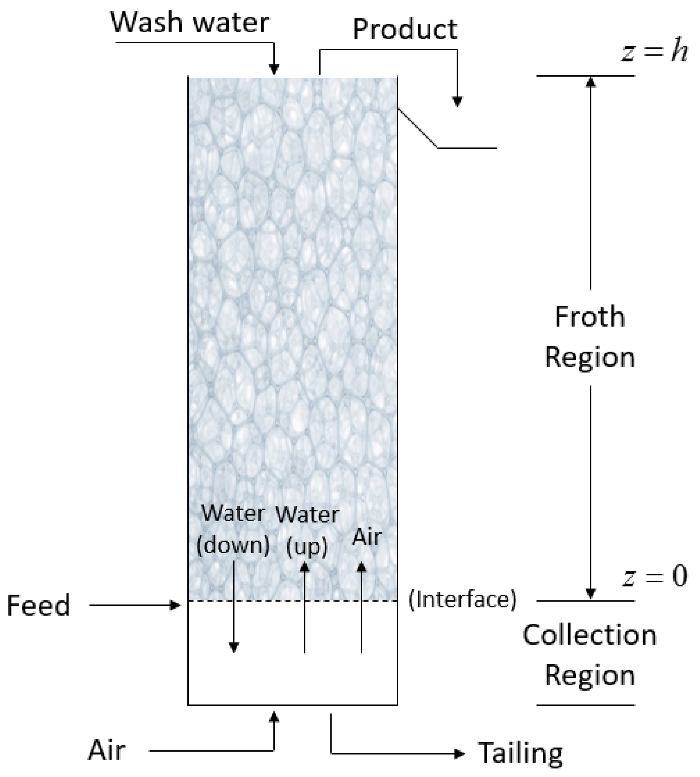
For the model predictive controller design, a three-phase column flotation dynamic model was developed. A typical column flotation process can be divided into two regions [3]: the collection region and the froth region (a schematic representation of the column flotation process is given in Figure 1). This work considers the collection region as a model given by the continuous stirred tank reactor (CSTR) and considers the froth region as a plug flow reactor (PFR) model. According to the mass balance laws, the overall column flotation system is described by a set of nonlinear heterodirectional coupled hyperbolic partial differential equations (PDEs) and ordinary differential equations (ODEs) that are connected through the PDEs’ boundaries. The steady-state profiles are utilized to linearize the original nonlinear system, and then the discrete model is realized by the Cayley–Tustin time discretization transformation [18,19,20]. By using this method, the continuous linear infinite-dimensional PDE system can be mapped into a discrete infinite-dimensional system without spatial discretization; the discretized model is structure-preserving and does not imply any model reduction [21]. Finally, the model predictive controller is designed on the basis of the infinite-dimensional discrete model. The paper is organized as follows: Section 2 develops the model of the column flotation process, and the discrete version of the system is obtained by using the Cayley–Tustin time discretization transformation. Section 3 addresses the model predictive controller design for the coupled PDE–ODE model with the consideration of input disturbance rejection and input and state/output constraints. Simulation results are shown in Section 4 to demonstrate the controller performance. Finally, Section 5 provides the conclusions.

2. Model Formulation of Column Flotation

2.1. Model Description

Column flotation utilizes the principle of countercurrent flow, in which air is introduced into the column at the bottom through a sparger or in the form of externally generated bubbles and rises through the downward-flowing slurry that contains mineral, locked, and gangue particles. By countercurrent flow, contact, and collision, hydrophobic particles (minerals) attach to the bubbles forming bubble–particle aggregates and reach the top of the column; they are subsequently removed at the top as a valuable product. Above the overflowing froth, there is a fine spray of water, washing down the undesired particles that could have been entrained by the bubbles from the froth region [22,23]. Meanwhile, rising bubbles entrain some water flow together through bubble coalescence, and the interaction of wash water and particles also simultaneously occurs. Therefore, the essential process step in column flotation is the transfer of particles between the water phase and air phase as well as between the upward and downward water phases.

On the basis of the above description and by making appropriate mass balances, the following equations are obtained to describe the column flotation process.

2.1.1. Model for Collection Region

Under the assumption of perfect mixing, the collection region can be considered as a CSTR, which means that the material properties are uniform throughout the reactor. Therefore, the model for the collection region is described by coupled ODEs. The state variables for the process of the collection region are mass concentrations of solid particles (mineral, locked, and gangue) with the air phase ($C_a$) and water phase ($C_w$):

$$\begin{array}{ccc}\hfill \frac{d\left(H_{a}V{C}_a\left(t\right)\right)}{dt}& =& \alpha Avf{H}_{w}V{C}_w\left(t\right)-\beta H_{a}V{C}_a\left(t\right)-Q_a{C}_a\left(t\right)\hfill \end{array}$$

(1)

$$\begin{array}{ccc}\hfill \frac{d\left(H_{w}V{C}_w\left(t\right)\right)}{dt}& =& -\alpha Avf{H}_{w}V{C}_w\left(t\right)+\beta H_{a}V{C}_a\left(t\right)+Q_F{C}_F-Q_T{C}_w\left(t\right)\hfill \\ & +& Q_{w_d}{C}_{w_d}(0,t)-Q_{w_u}{C}_w\left(t\right),\hfill \end{array}$$

(2)

where $f=1-\frac{C_a}{C_a^{*}}$ is the fractional free surface area of the bubbles; $Q_i=U_{i}Ac$ is the flow rate of i-th phase; $Q_a$ is the air flow rate; $Q_{w_u}$ is the upward water flow rate; $Q_{w_d}$ is the downward water flow rate; $Q_F$ is the feed flow rate; $Q_T$ is the tailing flow rate; $U_a$, $U_{w_u}$, $U_{w_d}$, $U_F$, $U_T$ are the velocities of particles with air, upward water, downward water, feed, and tailing phase, respectively. $Ac$ is the cross-sectional area of the column, V is the volume of the collection region, $H_a$ is the holdup of the air phase, $H_w$ is the holdup of the water phase, $\alpha$ is the particle–bubble attachment-rate parameter, $\beta$ is the particle–bubble detachment rate parameter, and $Av$ is the air–water interfacial area per unit volume of the column. The initial conditions for the ODE model of the collection region are given by

$$\begin{array}{c}\hfill C_a\left(0\right)=C_{a0},C_w\left(0\right)=C_{w0}.\end{array}$$

(3)

2.1.2. Model for Froth Region

The froth region can be considered as a PFR, which means that the material is perfectly mixed perpendicular to the direction of flow but is not mixed along the flow direction. This region is modeled by a set of transport hyperbolic PDEs. An upward water phase is added in this region because of the bubble entrainment. The state variables for the process of the froth region are mass concentrations of solid particles (mineral, locked, and gangue) with the air phase ($C_a^F$), downward water phase ($C_{w_d}$), and upward water phase ($C_{w_u}$).

$$\begin{array}{ccc}\hfill \frac{\partial \left(H_a{C}_a^F(z,t)\right)}{\partial t}& =& -\frac{\partial \left(U_a{C}_a^F(z,t)\right)}{\partial z}+\alpha Avf{C}_{w_d}(z,t)+\sigma Avf{C}_{w_u}(z,t)-\beta C_a^F(z,t),\hfill \end{array}$$

(4)

$$\begin{array}{ccc}\hfill \frac{\partial \left(H_{w_d}{C}_{w_d}(z,t)\right)}{\partial t}& =& \frac{\partial \left[(U_{w_d}+H_{w_d}{U}_s)C_{w_d}(z,t)\right]}{\partial z}-\alpha Avf{C}_{w_d}(z,t)+\rho C_{w_u}(z,t)+k\beta C_a^F(z,t),\hfill \end{array}$$

(5)

$$\begin{array}{ccc}\hfill \frac{\partial \left(H_{w_u}{C}_{w_u}(z,t)\right)}{\partial t}& =& -\frac{\partial \left(U_{w_u}{C}_{w_u}(z,t)\right)}{\partial z}-\sigma Avf{C}_{w_u}(z,t)-\rho C_{w_u}(z,t)+(1-k)\beta C_a^F(z,t).\hfill \end{array}$$

(6)

The letter F is marked in the upper right corner of the parameter $C_a$ to indicate that it is a froth region parameter that can be easily distinguished from the collection region parameter. The term $\alpha Avf{C}_{w_d}$ represents the transfer of particles from the downward water flow to the bubble, $\sigma Avf{C}_{w_u}$ represents the transfer of particles from the upward water flow to the bubble, $\beta C_a$ represents the particles’ detachment from the bubble, and $\rho C_{w_u}$ represents the transfer of particles from the upward water flow to the downward water flow. This transport-reaction model belongs to the class of fully state-coupled heterodirectional transport systems (transporting velocities have opposite signs).

The boundary and initial conditions for the PED model of the froth region are given by the following:

$$\begin{array}{ccc}\hfill C_a^F(0,t)& =& C_a\left(t\right),C_{w_u}(0,t)=C_w\left(t\right),C_{w_d}(h,t)=0.\hfill \end{array}$$

(7)

$$\begin{array}{ccc}\hfill C_a^F(z,0)& =& f_a\left(z\right),C_{w_u}(z,0)=f_{w_u}\left(z\right),C_{w_d}(z,0)=f_{w_d}\left(z\right).\hfill \end{array}$$

(8)

In the system given by Equations (1)–(8), the ODE system provides boundary conditions for the PDE system. The froth overflow (production) is controlled by the velocity of the feed; that is, the velocity of the feed $U_F$ is the control input and the mass concentration of solid particles with the air phase of froth overflow $C_a^F(h,t)$ is the output.

2.2. Linearized Model

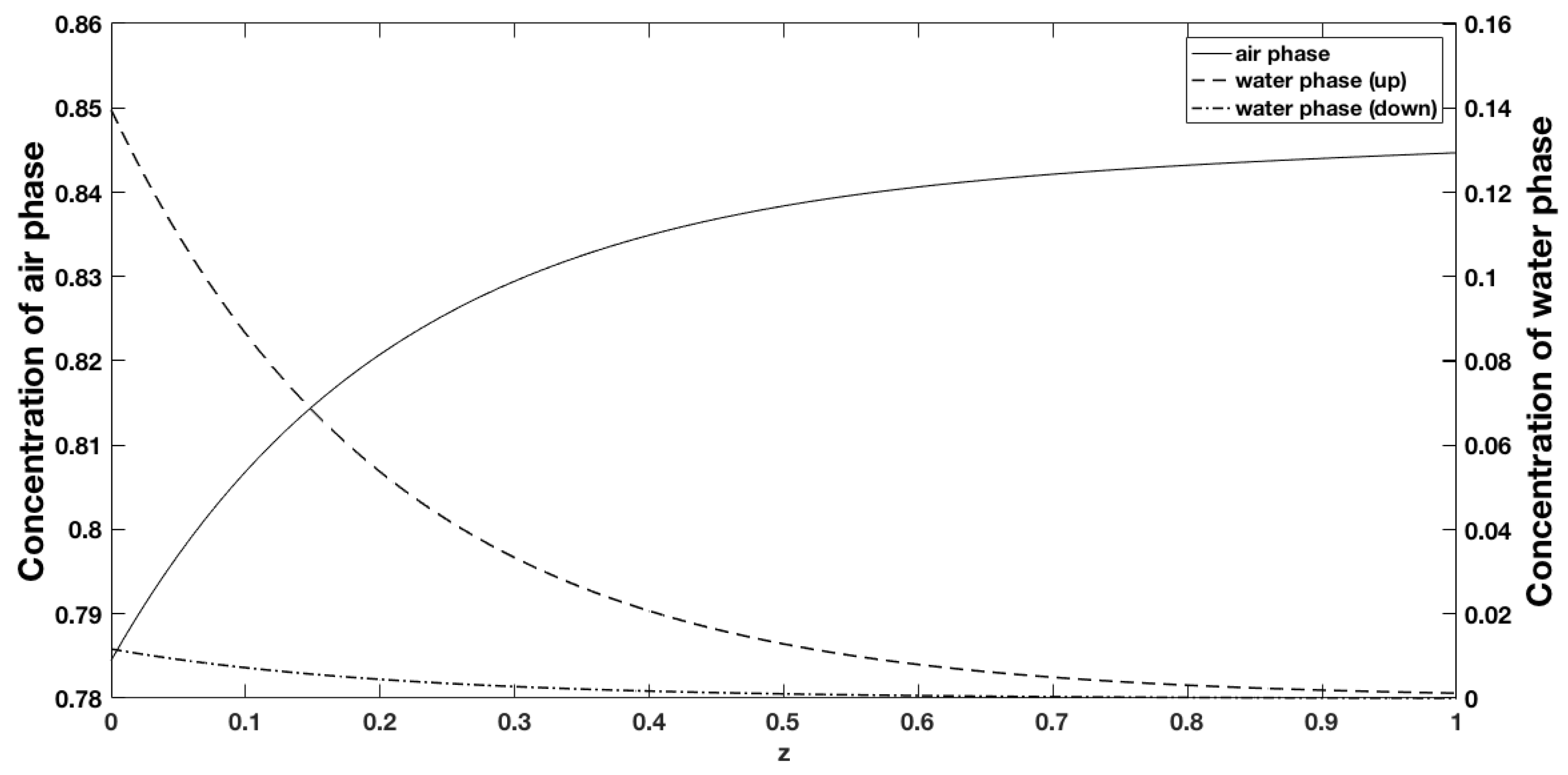
The system described by Equations (1)–(8) is nonlinear, and it is essential for it to be linearized for further analysis (taking the mineral, e.g., the steady-state profiles of the mineral within three phases are illustrated in Figure 2). $C_{as}$, $C_{w_{d}s}$, $C_{w_{u}s}$, and $U_{F0}$ are defined at steady state. With the consideration of steady-state conditions, defining the variables $C_a\left(t\right)=C_{as}\left(0\right)+x_{ab}\left(t\right)$, $C_w\left(t\right)=C_{w_{u}s}\left(0\right)+x_{wb}\left(t\right)$, $C_a^F(z,t)=C_{as}\left(z\right)+x_a(z,t)$, $C_{w_d}(z,t)=C_{w_{d}s}\left(z\right)+x_{w_d}(z,t)$, $C_{w_u}(z,t)=C_{w_{u}s}\left(z\right)+x_{w_u}(z,t)$, and $U_F=U_{F0}+u\left(t\right)$, one can obtain the following linear coupled PDE–ODEs:

$$\begin{array}{ccc}\hfill \frac{\partial }{\partial t}\left[\begin{array}{c}{x}_a(z,t)\\ x_{w_d}(z,t)\\ x_{w_u}(z,t)\end{array}\right]& =& \left[\begin{array}{ccc}-m_1\frac{\partial }{\partial z}+J_{11}\left(z\right)& J_{12}\left(z\right)& J_{13}\left(z\right)\\ J_{21}\left(z\right)& m_2\frac{\partial }{\partial z}+J_{22}\left(z\right)& J_{23}\left(z\right)\\ J_{31}\left(z\right)& J_{32}\left(z\right)& -m_3\frac{\partial }{\partial z}+J_{33}\left(z\right)\end{array}\right]\left[\begin{array}{c}{x}_a(z,t)\\ x_{w_d}(z,t)\\ x_{w_u}(z,t)\end{array}\right],\hfill \end{array}$$

(9)

$$\begin{array}{ccc}\hfill \frac{d}{dt}\left[\begin{array}{c}{x}_{ab}\left(t\right)\\ x_{wb}\left(t\right)\end{array}\right]& =& \left[\begin{array}{cc}{b}_{11}& b_{12}\\ b_{21}& b_{22}\end{array}\right]\left[\begin{array}{c}{x}_{ab}\left(t\right)\\ x_{wb}\left(t\right)\end{array}\right]+\left[\begin{array}{c}0\\ \frac{C_F}{H_{w}l}\end{array}\right]u\left(t\right)+\left[\begin{array}{c}0\\ \frac{U_{w_d}}{H_{w}l}\end{array}\right]x_{w_d}(0,t),\hfill \end{array}$$

(10)

with the following boundary conditions and initial conditions:

$$\begin{array}{c}\hfill x_a(0,t)=x_{ab}\left(t\right),x_{w_u}(0,t)=x_{wb}\left(t\right),x_{w_d}(h,t)=0;\end{array}$$

(11)

$$x_{ab}\left(0\right)=x_{ab0},x_{wb}\left(0\right)=x_{wb0},x_a(z,0)=x_{a0},x_{w_u}(z,0)=x_{w_{u}0},x_{w_d}(z,0)=x_{w_{d}0};$$

(12)

where $l=\frac{V}{Ac}$, $m_1=\frac{U_a}{H_a}$, $m_2=\frac{U_{w_d}+H_{w_d}{U}_s}{H_{w_d}}$, $m_3=\frac{U_{w_u}}{H_{w_u}}$, $b_{11}=-\beta -\frac{U_{a_b}}{H_{a_b}l}-\frac{\alpha Av{H}_w}{H_{a_b}{C}_a^{*}}{C}_{w_{u}s}\left(0\right)$, $b_{12}=\frac{\alpha Av{H}_w}{H_{a_b}}-\frac{\alpha Av{H}_w}{H_{a_b}{C}_a^{*}}{C}_{as}\left(0\right)$, $b_{21}=\frac{\beta H_{a_b}}{H_w}+\frac{\alpha Av}{C_a^{*}}{C}_{w_{u}s}\left(0\right)$, and $b_{22}=-\alpha Av-\frac{U_T}{H_{w}l}-\frac{U_{w_u}}{H_{w}l}+\frac{\alpha Av}{C_a^{*}}{C}_{as}\left(0\right)$. $J_{ij}\left(z\right)(i=1,2,3;j=1,2,3)$ is the Jacobian of the nonlinear term evaluated at steady state.

$$\begin{array}{ccc}\hfill J:& =& \left[\begin{array}{ccc}{J}_{11}\left(z\right)& J_{12}\left(z\right)& J_{13}\left(z\right)\\ J_{21}\left(z\right)& J_{22}\left(z\right)& J_{23}\left(z\right)\\ J_{31}\left(z\right)& J_{32}\left(z\right)& J_{33}\left(z\right)\end{array}\right]\hfill \\ & =& \left[\begin{array}{ccc}-\frac{\beta }{H_a}-\frac{\alpha Av}{H_a{C}_a^{*}}{C}_{w_{d}s}\left(z\right)-\frac{\sigma Av}{H_a{C}_a^{*}}{C}_{w_{u}s}\left(z\right)& \frac{\alpha Av}{H_a}-\frac{\alpha Av}{H_a{C}_a^{*}}{C}_{as}\left(z\right)& \frac{\sigma Av}{H_a}-\frac{\sigma Av}{H_a{C}_a^{*}}{C}_{as}\left(z\right)\\ \frac{k\beta }{H_{w_d}}+\frac{\alpha Av}{H_{w_d}{C}_a^{*}}{C}_{w_{d}s}\left(z\right)& -\frac{\alpha Av}{H_{w_d}}+\frac{\alpha Av}{H_{w_d}{C}_a^{*}}{C}_{as}\left(z\right)& \frac{\rho }{H_{w_d}}\\ \frac{(1-k)\beta }{H_{w_u}}+\frac{\sigma Av}{H_{w_u}{C}_a^{*}}{C}_{w_{u}s}\left(z\right)& 0& -\frac{\sigma Av}{H_{w_u}}+\frac{\sigma Av}{H_{w_u}{C}_a^{*}}{C}_{as}\left(z\right)-\frac{\rho }{H_{w_u}}\end{array}\right]\hfill \end{array}$$

(13)

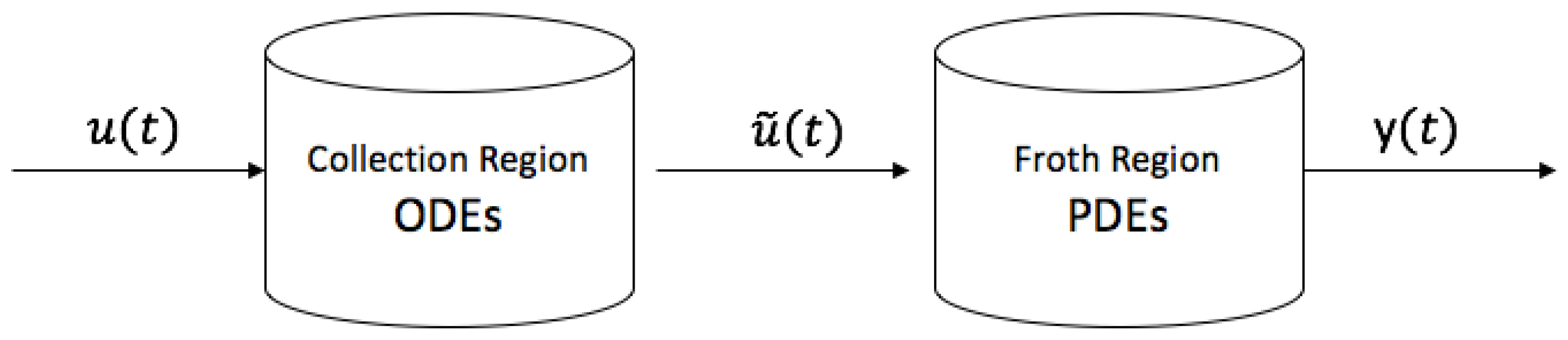
The interconnection of the hyperbolic PDE system and ODE system can be considered as the boundary-controlled hyperbolic PDE system (see Figure 3). The state transformation that transfers the boundary actuation to in-domain actuation is given as $x_a(z,t)={\overline{x}}_a(z,t)+B_1\left(z\right)x_a(0,t)$, and $x_{w_u}(z,t)={\overline{x}}_{w_u}(z,t)+B_2\left(z\right)x_{w_u}(0,t)$, with ${\overline{x}}_a(0,t)=0$, ${\overline{x}}_{w_u}(0,t)=0$, $B_1\left(0\right)=1$, and $B_2\left(0\right)=1$. Equations (9) and (10) become

$$\begin{array}{ccc}\hfill \frac{\partial {\overline{x}}_a(z,t)}{\partial t}& =& -m_1\frac{\partial {\overline{x}}_a(z,t)}{\partial z}+J_{11}\left(z\right){\overline{x}}_a(z,t)+J_{12}\left(z\right)x_{w_d}(z,t)+J_{13}\left(z\right){\overline{x}}_{w_u}(z,t)\hfill \\ & +& [J_{13}\left(z\right)B_2\left(z\right)-b_{12}{B}_1\left(z\right)]x_{w_u}(0,t)+[-m_1\frac{d{B}_1\left(z\right)}{dz}-b_{11}{B}_1\left(z\right)+J_{11}\left(z\right)B_1\left(z\right)]x_a(0,t),\hfill \end{array}$$

(14)

$$\begin{array}{ccc}\hfill \frac{\partial x_{w_d}(z,t)}{\partial t}& =& m_2\frac{\partial x_{w_d}(z,t)}{\partial z}+J_{21}\left(z\right){\overline{x}}_a(z,t)+J_{22}\left(z\right)x_{w_d}(z,t)+J_{23}\left(z\right){\overline{x}}_{w_u}(z,t)\hfill \\ & +& [J_{21}\left(z\right)B_1\left(z\right)x_a(0,t)+J_{23}\left(z\right)B_2\left(z\right)x_{w_u}(0,t)],\hfill \end{array}$$

(15)

$$\begin{array}{ccc}\hfill \frac{\partial {\overline{x}}_{w_u}(z,t)}{\partial t}& =& -m_3\frac{\partial {\overline{x}}_{w_u}(z,t)}{\partial z}+J_{31}\left(z\right){\overline{x}}_a(z,t)+J_{32}\left(z\right)x_{w_d}(z,t)+J_{33}\left(z\right){\overline{x}}_{w_u}(z,t)\hfill \\ & +& [J_{31}\left(z\right)B_1\left(z\right)-b_{21}{B}_2\left(z\right)]x_a(0,t)+[-m_3\frac{d{B}_2\left(z\right)}{dz}-b_{22}{B}_2\left(z\right)+J_{33}\left(z\right)B_2\left(z\right)]x_{w_u}(0,t)\hfill \\ \hfill & -& B_2\left(z\right)\frac{U_{w_d}}{H_{w}l}{x}_{w_d}(0,t)-B_2\left(z\right)\frac{C_F}{H_{w}l}u\left(t\right),\hfill \end{array}$$

(16)

$$\begin{array}{ccc}\hfill \frac{d{x}_{ab}\left(t\right)}{dt}& =& b_{11}{x}_{ab}\left(t\right)+b_{12}{x}_{wb}\left(t\right),\hfill \end{array}$$

(17)

$$\begin{array}{ccc}\hfill \frac{d{x}_{wb}\left(t\right)}{dt}& =& b_{21}{x}_{ab}\left(t\right)+b_{22}{x}_{wb}\left(t\right)+\frac{U_{w_d}}{H_{w}l}{x}_{w_d}(0,t)+\frac{C_F}{H_{w}l}u\left(t\right),\hfill \end{array}$$

(18)

with the following boundary conditions and initial conditions:

$$\begin{array}{c}{\overline{x}}_a(0,t)=0,{\overline{x}}_{w_u}(0,t)=0,x_{w_d}(h,t)=0;\end{array}$$

(19)

$$x_{ab}\left(0\right)=x_{ab0},x_{wb}\left(0\right)=x_{wb0},{\overline{x}}_a(z,0)={\overline{x}}_{a0},{\overline{x}}_{w_u}(z,0)={\overline{x}}_{w_{u}0},x_{w_d}(z,0)=x_{w_{d}0};$$

(20)

with ${\overline{x}}_{a0}=x_a(z,0)-B_1\left(z\right)x_{ab}\left(0\right)$ and ${\overline{x}}_{w_{u}0}=x_{w_u}(z,0)-B_2\left(z\right)x_{wb}\left(0\right)$. We consider the conditions $-m_1\frac{d{B}_1\left(z\right)}{dz}-b_{11}{B}_1\left(z\right)+J_{11}\left(z\right)B_1\left(z\right)=0$ and $-m_3\frac{d{B}_2\left(z\right)}{dz}-b_{22}{B}_2\left(z\right)+J_{33}\left(z\right)B_2\left(z\right)=0$ and solve for the $B_1\left(z\right)$ and $B_2\left(z\right)$ expressions, which simplifies the system given by Equations (14)–(18) as follows:

$$\begin{array}{ccc}\hfill \frac{\partial {\overline{x}}_a(z,t)}{\partial t}& =& -m_1\frac{\partial {\overline{x}}_a(z,t)}{\partial z}+J_{11}\left(z\right){\overline{x}}_a(z,t)+J_{12}\left(z\right)x_{w_d}(z,t)+J_{13}\left(z\right){\overline{x}}_{w_u}(z,t)\hfill \\ & +& [J_{13}\left(z\right)B_2\left(z\right)-b_{12}{B}_1\left(z\right)]x_{wb}\left(t\right),\hfill \end{array}$$

(21)

$$\begin{array}{ccc}\hfill \frac{\partial x_{w_d}(z,t)}{\partial t}& =& m_2\frac{\partial x_{w_d}(z,t)}{\partial z}+J_{21}\left(z\right){\overline{x}}_a(z,t)+J_{22}\left(z\right)x_{w_d}(z,t)+J_{23}\left(z\right){\overline{x}}_{w_u}(z,t)\hfill \\ & +& J_{21}\left(z\right)B_1\left(z\right)x_{ab}\left(t\right)+J_{23}\left(z\right)B_2\left(z\right)x_{wb}\left(t\right),\hfill \end{array}$$

(22)

$$\begin{array}{ccc}\hfill \frac{\partial {\overline{x}}_{w_u}(z,t)}{\partial t}& =& -m_3\frac{\partial {\overline{x}}_{w_u}(z,t)}{\partial z}+J_{31}\left(z\right){\overline{x}}_a(z,t)+J_{32}\left(z\right)x_{w_d}(z,t)+J_{33}\left(z\right){\overline{x}}_{w_u}(z,t)\hfill \\ & +& [J_{31}\left(z\right)B_1\left(z\right)-b_{21}{B}_2\left(z\right)]x_{ab}\left(t\right)-B_2\left(z\right)\frac{U_{w_d}}{H_{w}l}{x}_{w_d}(0,t)-B_2\left(z\right)\frac{C_F}{H_{w}l}u\left(t\right),\hfill \end{array}$$

(23)

$$\begin{array}{ccc}\hfill \frac{d{x}_{ab}\left(t\right)}{dt}& =& b_{11}{x}_{ab}\left(t\right)+b_{12}{x}_{wb}\left(t\right),\hfill \end{array}$$

(24)

$$\begin{array}{ccc}\hfill \frac{d{x}_{wb}\left(t\right)}{dt}& =& b_{21}{x}_{ab}\left(t\right)+b_{22}{x}_{wb}\left(t\right)+\frac{U_{w_d}}{H_{w}l}{x}_{w_d}(0,t)+\frac{C_F}{H_{w}l}u\left(t\right).\hfill \end{array}$$

(25)

We consider the extended state $x\in H⨁R^n$, where H is a real Hilbert space $L_2(0,1)$ with the inner product $<·,·>$ and $R^n$ is a real space. The input $u\left(t\right)\in U$; the disturbance $g\left(t\right)\in G$; and the output $y\left(t\right)\in Y$, U, G, and Y are real Hilbert spaces. The system given by Equations (21)–(25) can be expressed as the equivalent state-space description:

$$\begin{array}{ccc}\hfill \dot{x}\left(t\right)& =& Ax\left(t\right)+Bu\left(t\right)+Eg\left(t\right),\hfill \end{array}$$

(26)

where the system state is $x(·,t)={\left[{\overline{x}}_a(z,t),x_{w_d}(z,t),{\overline{x}}_{w_u}(z,t),x_{ab}\left(t\right),x_{wb}\left(t\right)\right]}^T$ and the disturbance is $g\left(t\right)=x_{w_d}(0,t)$. The system operator A is defined on its domain as $D\left(A\right)=\left\{x={[x_1,x_2,x_3,x_4,x_5]}^T\in H:xisa.c.,\frac{dx}{dz}\in H,x_1\left(0\right)=0,x_2\left(h\right)=0,x_3\left(0\right)=0\right\}$ by

$$\begin{array}{ccc}\hfill A& =& \left[\begin{array}{cc}{A}_F& A_O\\ 0& A_C\end{array}\right]\hfill \\ \hfill & =& \left[\begin{array}{ccccc}-m_1\frac{\partial }{\partial z}+J_{11}\left(z\right)& J_{12}\left(z\right)& J_{13}\left(z\right)& 0& J_{13}\left(z\right)B_2\left(z\right)-b_{12}{B}_1\left(z\right)\\ J_{21}\left(z\right)& m_2\frac{\partial }{\partial z}+J_{22}\left(z\right)& J_{23}\left(z\right)& J_{21}\left(z\right)B_1\left(z\right)& J_{23}\left(z\right)B_2\left(z\right)\\ J_{31}\left(z\right)& J_{32}\left(z\right)& -m_3\frac{\partial }{\partial z}+J_{33}\left(z\right)& J_{31}\left(z\right)B_1\left(z\right)-b_{21}{B}_2\left(z\right)& 0\\ 0& 0& 0& b_{11}& b_{12}\\ 0& 0& 0& b_{21}& b_{22}\end{array}\right].\hfill \end{array}$$

(27)

The input, disturbance, and output operators are given by $B=\left[\begin{array}{c}0\\ 0\\ -B_2\left(z\right)\frac{C_F}{H_{w}l}\\ 0\\ \frac{C_F}{H_{w}l}\end{array}\right]$ and $E=\left[\begin{array}{c}0\\ 0\\ -B_2\left(z\right)\frac{U_{w_d}}{H_{w}l}\\ 0\\ \frac{U_{w_d}}{H_{w}l}\end{array}\right]$.

2.3. Discretized Model

For the discrete controller design, a discretized model is required. Cayley–Tustin time discretization transformation is used to obtain discrete models without consideration of spatial discretization and/or without any other type of model spatial approximation.

2.3.1. Time Discretization for Linear PDE

The linear infinite-dimensional system is described by the following state-space system:

$$\begin{array}{ccc}\hfill \dot{x}(z,t)& =& Ax(z,t)+Bu\left(t\right),x(z,0)=x_0;\hfill \\ \hfill y\left(t\right)& =& Cx(z,t)+Du\left(t\right).\hfill \end{array}$$

(28)

The operator $A:D\left(A\right)\subset H\to H$ is a generator of a $C_0$-semigroup on H and has a Yoshida extension operator $A_{-1}$. $B,C,$ and D are linear operators associated with the actuation and output measurement or direct feed-forward element; that is, $B\subset L(U,H)$, $C\subset L(H,Y)$, and $D\subset L(U,Y)$. Given a time discretization parameter $d>0$, the Tustin time discretization is given by the following [24]:

$$\begin{array}{ccc}\hfill \frac{x\left(jd\right)-x\left(\right(j-1\left)d\right)}{d}& \approx & A\frac{x\left(jd\right)+x\left(\right(j-1\left)d\right)}{2}+Bu\left(jd\right),\hfill \\ \hfill y\left(jd\right)& \approx & C\frac{x\left(jd\right)+x\left(\right(j-1\left)d\right)}{2}+Du\left(jd\right),\hfill \\ \hfill x\left(0\right)& =& x_0.\hfill \end{array}$$

(29)

We let $u_j^d/\sqrt{d}$ be an approximation to $u\left(jd\right)$, under the assumptions that $y_j^d/\sqrt{d}$ converges to $y\left(jd\right)$ as $d\to 0$. Then, one obtains discrete time dynamics as follows:

$$\begin{array}{ccc}\hfill \frac{x_j^d-x_{j-1}^d}{d}& =& A\frac{x_j^d+x_{j-1}^d}{2}+B{u}_j^d/\sqrt{d},\hfill \\ \hfill y_j^d/\sqrt{d}& =& C\frac{x_j^d+x_{j-1}^d}{2}+D{u}_j^d/\sqrt{d},\hfill \\ \hfill x_0^d& =& x_0.\hfill \end{array}$$

(30)

After some calculations, one obtains the form of a discrete system:

$$\begin{array}{ccc}\hfill x(z,k)& =& A_{d}x(z,k-1)+B_{d}u\left(k\right),x(z,0)=x_0;\hfill \\ \hfill y\left(k\right)& =& C_{d}x(z,k-1)+D_{d}u\left(k\right).\hfill \end{array}$$

(31)

Here $\delta =2/d$, and the operators $A_d$, $B_d$, $C_d$, and $D_d$ are given by

$$\begin{array}{c}\hfill \left[\begin{array}{cc}{A}_d& B_d\\ C_d& D_d\end{array}\right]=\left[\begin{array}{cc}{[\delta -A]}^{-1}[\delta +A]& \sqrt{2\delta }{[\delta -A]}^{-1}B\\ \sqrt{2\delta }C{[\delta -A]}^{-1}& G\left(\delta \right)\end{array}\right],\end{array}$$

(32)

where $G\left(\delta \right)$ denotes the transfer function of the system, $G\left(\delta \right)=C{[\delta -A]}^{-1}B+D$. Operator $A_d$ can be expressed as $A_d=-I+2\delta {[\delta -A]}^{-1}$, where I is the identity operator. By introducing the affine disturbance input, the time discretization for the most general form:

$$\begin{array}{ccc}\hfill \dot{x}(z,t)& =& Ax(z,t)+Bu\left(t\right)+Eg\left(t\right),x(z,0)=x_0,\hfill \\ \hfill y\left(t\right)& =& Cx(z,t)+Du\left(t\right)+Fg\left(t\right),\hfill \end{array}$$

(33)

is given by [25]; the corresponding discrete operator of the linear operators $E\subset L(R^n,H)$ and $F\subset L(R^n,Y)$ are $E_d=\sqrt{2\delta }{[\delta -A]}^{-1}E$ and $F_d=C{[\delta -A]}^{-1}E+F$.

2.3.2. Time Discretization of Column Flotation System

From the previous section, one can find resolvent $R(\delta ,A)={[\delta -A]}^{-1}$ of the column operator A (Equation (27)), which provides discrete operators ($A_d,B_d,C_d,$ and $D_d$) to be easily realized. Returning to the system given by Equation (26), the resolvent operator can be obtained by taking a Laplace transform. After the Laplace transform, one obtains

$$\begin{array}{ccc}\hfill \frac{\partial {\overline{x}}_a(z,s)}{\partial z}& =& \frac{1}{m_1}(J_{11}\left(z\right)-s){\overline{x}}_a(z,s)+\frac{1}{m_1}{J}_{12}\left(z\right)x_{w_d}(z,s)+\frac{1}{m_1}{J}_{13}\left(z\right){\overline{x}}_{w_u}(z,s)\hfill \\ \hfill & +& \frac{1}{m_1}[J_{13}\left(z\right)B_2\left(z\right)-b_{12}{B}_1\left(z\right)]x_{w_u}(0,s)+\frac{1}{m_1}{\overline{x}}_a(z,0),\hfill \end{array}$$

(34)

$$\begin{array}{ccc}\hfill \frac{\partial x_{w_d}(z,s)}{\partial z}& =& -\frac{1}{m_2}{J}_{21}\left(z\right){\overline{x}}_a(z,s)-\frac{1}{m_2}(J_{22}\left(z\right)-s)x_{w_d}(z,s)-\frac{1}{m_2}{J}_{23}\left(z\right){\overline{x}}_{w_u}(z,s)\hfill \\ \hfill & -& \frac{1}{m_2}{J}_{21}\left(z\right)B_1\left(z\right)x_a(0,s)-\frac{1}{m_2}{J}_{23}\left(z\right)B_2\left(z\right)x_{w_u}(0,s)-\frac{1}{m_2}{x}_{w_d}(z,0),\hfill \end{array}$$

(35)

$$\begin{array}{ccc}\hfill \frac{\partial {\overline{x}}_{w_u}(z,s)}{\partial z}& =& \frac{1}{m_3}{J}_{31}\left(z\right){\overline{x}}_a(z,s)+\frac{1}{m_3}{J}_{32}\left(z\right)x_{w_d}(z,s)+\frac{1}{m_3}(J_{33}\left(z\right)-s){\overline{x}}_{w_u}(z,s)\hfill \\ \hfill & +& \frac{1}{m_3}[J_{31}\left(z\right)B_1\left(z\right)-b_{21}{B}_2\left(z\right)]x_a(0,s)+\frac{1}{m_3}{\overline{x}}_{w_u}(z,0),\hfill \end{array}$$

(36)

$$\begin{array}{ccc}\hfill x_{ab}\left(s\right)& =& \frac{s-b_{22}}{b}{x}_{ab}\left(0\right)+\frac{b_{12}}{b}{x}_{wb}\left(0\right),\hfill \end{array}$$

(37)

$$\begin{array}{ccc}\hfill x_{wb}\left(s\right)& =& \frac{b_{21}}{b}{x}_{ab}\left(0\right)+\frac{s-b_{11}}{b}{x}_{wb}\left(0\right),\hfill \end{array}$$

(38)

where $b=(s-b_{11})(s-b_{22})-b_{21}{b}_{12}$.

By solving this ODE, one obtains

$$\begin{array}{c}\hfill \left[\begin{array}{c}{\overline{x}}_a(z,s)\\ x_{w_d}(z,s)\\ {\overline{x}}_{w_u}(z,s)\end{array}\right]=e^{\overline{A}z}\left[\begin{array}{c}{\overline{x}}_a(0,s)\\ x_{w_d}(0,s)\\ {\overline{x}}_{w_u}(0,s)\end{array}\right]+{\int }_0^z{e}^{\overline{A}(z-\eta )}\left[\begin{array}{c}\frac{1}{m_1}{\overline{x}}_a(\eta ,0)+\frac{1}{m_1}{J}_{a1}\left(\eta \right)x_{ab}\left(0\right)+\frac{1}{m_1}{J}_{a2}\left(\eta \right)x_{wb}\left(0\right)\\ -\frac{1}{m_2}{x}_{wd}(\eta ,0)-\frac{1}{m_2}{J}_{d1}\left(\eta \right)x_{ab}\left(0\right)-\frac{1}{m_2}{J}_{d2}\left(\eta \right)x_{wb}\left(0\right)\\ \frac{1}{m_3}{\overline{x}}_{w_u}(\eta ,0)+\frac{1}{m_3}{J}_{u1}\left(\eta \right)x_{ab}\left(0\right)+\frac{1}{m_3}{J}_{u2}\left(\eta \right)x_{wb}\left(0\right)\end{array}\right]d\eta ,\end{array}$$

(39)

where $J_{a1}\left(z\right)=\frac{b_{21}}{b}[J_{13}\left(z\right)B_2\left(z\right)-b_{12}{B}_1\left(z\right)]$, $J_{a2}\left(z\right)=\frac{s-b_{11}}{b}[J_{13}\left(z\right)B_2\left(z\right)-b_{12}{B}_1\left(z\right)]$, $J_{d1}\left(z\right)=\frac{s-b_{22}}{b}{J}_{21}\left(z\right)B_1\left(z\right)+\frac{b_{21}}{b}{J}_{23}\left(z\right)B_2\left(z\right)$, $J_{d2}\left(z\right)=\frac{b_{12}}{b}{J}_{21}\left(z\right)B_1\left(z\right)+\frac{s-b_{11}}{b}{J}_{23}\left(z\right)B_2\left(z\right)$, $J_{u1}\left(z\right)=\frac{s-b_{22}}{b}[J_{31}\left(z\right)B_1\left(z\right)-b_{21}{B}_2\left(z\right)]$, and $J_{u2}\left(z\right)=\frac{b_{12}}{b}[J_{31}\left(z\right)B_1\left(z\right)-b_{21}{B}_2\left(z\right)]$. For simplicity, we let $J_{ij}$, which is defined as a spatial average of $J_{ij}\left(z\right)$, replace $J_{ij}\left(z\right)$, so that the matrix exponential of $\overline{A}$ can be computed directly. Then, $\overline{A}=\left[\begin{array}{ccc}\frac{1}{m_1}(J_{11}-s)& \frac{1}{m_1}{J}_{12}& \frac{1}{m_1}{J}_{13}\\ -\frac{1}{m_2}{J}_{21}& -\frac{1}{m_2}(J_{22}-s)& -\frac{1}{m_2}{J}_{23}\\ \frac{1}{m_3}{J}_{31}& \frac{1}{m_3}{J}_{32}& \frac{1}{m_3}(J_{33}-s)\end{array}\right]$.

With the boundary conditions given by Equation (19), the resolvent of operator A can be expressed as follows:

$$\begin{array}{ccc}\hfill R(s,A)& =& {[sI-A]}^{-1}x(z,0)\hfill \\ & =& \left[\begin{array}{ccccc}{R}_{11}& R_{12}& R_{13}& R_{14}& R_{15}\\ R_{21}& R_{22}& R_{23}& R_{24}& R_{25}\\ R_{31}& R_{32}& R_{33}& R_{34}& R_{35}\\ 0& 0& 0& R_{44}& R_{45}\\ 0& 0& 0& R_{54}& R_{55}\end{array}\right]x(z,0),\hfill \end{array}$$

(40)

where $R_{11}$, $R_{12}$, ..., $R_{55}$ are shown in Appendix A. Then, the discretized model of the column flotation process takes the following form:

$$\begin{array}{ccc}\hfill x(z,k)& =& A_{d}x(z,k-1)+B_{d}u\left(k\right)+E_{d}g\left(k\right).\hfill \end{array}$$

(41)

3. Model Predictive Control Design

In this work, the model for the column flotation process uses coupled PDEs and ODEs with input disturbance $g\left(t\right)$; the continuous linearized model described in Equation (26) can be rewritten as

$$\begin{array}{ccc}\hfill \dot{x}\left(t\right)& =& Ax\left(t\right)+B\overline{u}\left(t\right),\hfill \end{array}$$

(42)

where $\overline{u}\left(t\right)=u\left(t\right)+\frac{U_{w_d}}{C_F}g\left(t\right)$. The discrete version is obtained by applying Cayley–Tustin discretization as follows:

$$\begin{array}{ccc}\hfill x(z,k)& =& A_{d}x(z,k-1)+B_d\overline{u}\left(k\right),\hfill \end{array}$$

(43)

where we have adopted $x(z,k)$ notation to denote spatial characteristics of the extended state $x\left(t\right)$. The model predictive controller was developed as a solution of the optimization problem by minimizing the following open-loop performance objective function across the length of the infinite horizon at sampling time k [26] on the basis of the above system given by Equation (43) without disturbances being present.

$$\begin{array}{cc}\hfill \underset{{\overline{u}}^N}{min}& \sum _{j=0}^{\infty }[<x(z,k+j|k),Qx(z,k+j|k)>\hfill \\ & +<\overline{u}(k+j+1|k),R\overline{u}(k+j+1|k)>]\hfill \\ \hfill s.t.& x(z,k+j|k)=A_{d}x(z,k+j-1|k)+B_d\overline{u}(k+j|k)]\hfill \\ & {\overline{u}}^{min}\le \overline{u}(k+j|k)\le {\overline{u}}^{max}\hfill \\ & x^{min}\le x(z,k+j|k)\le x^{max},\hfill \end{array}$$

(44)

where Q is a symmetric positive semidefinite matrix and R is a symmetric positive definite matrix. The infinite-horizon open-loop objective function in Equation (44) can be expressed as the finite-horizon open-loop objective function with $u(k+N+1|k)=0$, as below:

$$\begin{array}{cc}\hfill \underset{{\overline{u}}^N}{min}& J=\sum _{j=0}^{N-1}[<x(z,k+j|k),Qx(z,k+j|k)>\hfill \\ & +<\overline{u}(k+j+1|k),R\overline{u}(k+j+1|k)>]\hfill \\ & +<x(z,k+N|k),\overline{Q}x(z,k+N|k)>\hfill \\ \hfill s.t.& x(z,k+j|k)=A_{d}x(z,k+j-1|k)+B_d\overline{u}(k+j|k)\hfill \\ & {\overline{u}}^{min}\le \overline{u}(k+j|k)\le {\overline{u}}^{max}\hfill \\ & x^{min}\le x(z,k+j|k)\le x^{max},\hfill \end{array}$$

(45)

where $\overline{Q}$ is defined as the infinite sum $\overline{Q}={\sum }_{i=0}^{\infty }{A}_d^{*i}{C}_d^{*}Q{C}_d{A}_d^i$. This terminal state penalty operator $\overline{Q}$ can be calculated from the solution of the following discrete Lyapunov function:

$$A_d^{*}\overline{Q}{A}_d-\overline{Q}=-C_d^{*}Q{C}_d.$$

(46)

It can be noticed that operator $A_d$ in the equation is applied to some function and that the same holds for $C_d$; thus to derive $\overline{Q}$ directly from Equation (46) is not a feasible task. However, the unique solution of the discrete Lyapunov function can be related to the solution of the continuous Lyapunov function, which can be solved uniquely. Therefore, $\overline{Q}$ can be obtained by solving the continuous Lyapunov function:

$$A^{*}\overline{Q}+\overline{Q}A=-C^{*}QC,\overline{Q}\in D\left(A^{*}\right).$$

(47)

Proof. 

We establish a link between the continuous and discrete Lyapunov functions. If the continuous Lyapunov function holds, defining $A_d:=-I+2\delta {[\delta -A]}^{-1}$ and $A_d^{*}:={[-I+2\delta {[\delta -A]}^{-1}]}^{*}$, then

$$\begin{array}{ccc}\hfill A_d^{*}\overline{Q}{A}_d-\overline{Q}& =& {\left[-I+2\delta {(\delta -A)}^{-1}\right]}^{*}Q\left[-I+2\delta {(\delta -A)}^{-1}\right]-\overline{Q}\hfill \\ & =& {(\delta -A)}^{-1*}{[[-(\delta -A)+2\delta ]}^{*}Q[-(\delta -A)+2\delta ]\hfill \\ & -& {(\delta -A)}^{*}{Q(\delta -A)](\delta -A)}^{-1}\hfill \\ & =& {(\delta -A)}^{-1*}\left[2A^{*}\overline{Q}\delta +2\delta \overline{Q}A\right]{(\delta -A)}^{-1}\hfill \\ & =& {(\delta -A)}^{-1*}\left[2\delta (-C^{*}QC)\right]{(\delta -A)}^{-1}\hfill \\ & =& -{\left(\sqrt{2\delta }C{\left[\delta -A\right]}^{-1}\right)}^{*}Q\left(\sqrt{2\delta }C{\left[\delta -A\right]}^{-1}\right)\hfill \\ & =& -C_d^{*}Q{C}_d,\hfill \end{array}$$

such that the unique solution of the continuous Lyapunov function (Equation (51)) is also a solution of the discrete Lyapunov function ((Equation 46)). ☐

Because of the fact that $\overline{u}\left(t\right)=u\left(t\right)+\frac{U_{w_d}}{C_F}g\left(t\right)$, straightforward algebraic manipulation of the objective function presented in Equation (45) results in the following program:

$$\begin{array}{ccc}\hfill \underset{U}{min}J& =& U^T<I,H>U+2U^T[<I,Px(z,k|k)>+<I,R\frac{U_{w_d}}{C_F}G>]\hfill \\ & +& <x(z,k|k),\overline{Q}x(z,k|k)>+<\frac{U_{w_d}}{C_F}G,R\frac{U_{w_d}}{C_F}G>,\hfill \end{array}$$

(48)

where $U={[u(k+1|k),u(k+2|k),\dots ,u(k+N|k)]}^T$, $G={[g(k+1|k),g(k+2|k),\dots ,g(k+N|k)]}^T$, and $H=\left[\begin{array}{cccc}{B}_d^{*}\overline{Q}{B}_d+R& B_d^{*}{A}_d^{*}\overline{Q}{B}_d& \cdots & B_d^{*}{A}_d^{*N-1}\overline{Q}{B}_d\\ B_d^{*}\overline{Q}{A}_d{B}_d& B_d^{*}\overline{Q}{B}_d+R& \cdots & B_d^{*}{A}_d^{*N-2}\overline{Q}{B}_d\\ ⋮& ⋮& \ddots & ⋮\\ B_d^{*}\overline{Q}{A}_d^{N-1}{B}_d& B_d^{*}\overline{Q}{A}_d^{N-2}{B}_d& \cdots & B_d^{*}\overline{Q}{B}_d+R\end{array}\right]$, $P=\left[\begin{array}{c}{B}_d^{*}\overline{Q}{A}_d\\ B_d^{*}\overline{Q}{A}_d^2\\ ⋮\\ B_d^{*}\overline{Q}{A}_d^N\end{array}\right]$.

The objective function is subjected to the following constraints:

$$\begin{array}{c}{\overline{U}}^{min}\le U+\frac{U_{w_d}}{C_F}G\le {\overline{U}}^{max},\hfill \\ X^{min}\le S(U+\frac{U_{w_d}}{C_F}G)+Tx(z,k|k)\le X^{max}.\hfill \end{array}$$

(49)

That is,

$$\begin{array}{c}\hfill \left[\begin{array}{c}I\\ -I\\ S\\ -S\end{array}\right]U\le \left[\begin{array}{c}{\overline{U}}^{max}-\frac{U_{w_d}}{C_F}G\\ -{\overline{U}}^{min}+\frac{U_{w_d}}{C_F}G\\ X^{max}-Tx(z,k|k)-S\frac{U_{w_d}}{C_F}G\\ -X^{min}+Tx(z,k|k)+S\frac{U_{w_d}}{C_F}G\end{array}\right],\end{array}$$

(50)

where $S=\left[\begin{array}{cccc}{B}_d& 0& \cdots & 0\\ A_d{B}_d& B_d& \cdots & 0\\ ⋮& ⋮& \ddots & ⋮\\ A_d^{N-1}{B}_d& A_d^{N-2}{B}_d& \cdots & B_d\end{array}\right]$ and $T=\left[\begin{array}{c}{A}_d\\ A_d^2\\ ⋮\\ A_d^N\end{array}\right]$.

The optimization problem described in Equation (48) is a standard finite-dimensional quadratic optimization problem, as inner products in Equation (48) are integrations over the spatial components in the cost function.

Remark 1.

The model predictive controller design in this paper uses the system state $x(z,t)$; therefore, it is necessary to design a discrete observer to reconstruct the system state. At present, the design of the continuous system observer is very mature, and it is feasible to design a discrete observer on this basis of the discrete infinite-dimensional model.

4. Simulation Results

In this section, the performance of the proposed model predictive control to keep the output at the steady state within the constraint range by adjusting the input is demonstrated by a comparison between high-fidelity numerical simulations of open-loop and controlled system responses.

In the simulations, the values of the system parameters were as given in

Table 1. Model parameters for both collection region (C) and froth region (F).

Symbol	Description	Value
h	Height of froth region	1.0
l	Height of collection region	1.0
$C{a}^{*}$	Bubble saturation parameter	5
$Av$	Air–water interfacial area	C: 1.0; F: 0.3
$U_w$	Water velocity of collection region	0.8
$U_s$	Settling/slip velocity	1
$H_a$	Air holdup	C: 0.3; F: 0.7
$H_{w_d}$	Downward water holdup	0.1
$H_{w_u}$	Upward water holdup	C: 0.7; F: 0.2
$U_a$	Air velocity	C: 0.1; F: 0.2
$U_{w_d}$	Downward water velocity	0.1
$U_{w_u}$	Upward water velocity	C: 0.08; F: 0.1
$\alpha$	Attachment-rate parameter for downward water	C: 1.2; F: 1.0
$\sigma$	Attachment-rate parameter for upward water	1.5
$\beta$	Detachment rate parameter	C: 0.1; F: 0
$\rho$	Transfer rate from upward water to downward water	0.1
k	Transfer rate from air to downward water	0.01
$a_1$, $a_2$, $a_3$	Initial-condition coefficients	$a_1=0.8$, $a_2=0.1$, $a_3=0.2$

. The time discretization parameter was chosen as $d=0.2$, which implies that $\delta =10$ and $\Delta z=0.01$ were chosen for the numerical integration.

In this work, C was considered as $C=I$, which implies that the full state was available for the controller realization, and thus $C^{*}=C$. The above framework allows for easy extension to the discrete observer design with boundary measurements applied; that is, $C(·):={\int }_0^1\delta (z-1)(·)dz$. The $\overline{Q}$ can be obtained by solving the following continuous Lyapunov equation corresponding to the discrete Lyapunov Equation (46):

$$A^{*}\overline{Q}+\overline{Q}A=-Q.$$

(51)

We consider $\overline{Q}=\left[\begin{array}{cc}{\overline{Q}}_1& 0\\ 0& {\overline{Q}}_2\end{array}\right]$, where ${\overline{Q}}_1\in H$, ${\overline{Q}}_2\in R^n$, and assume $Q=\left[\begin{array}{cc}{Q}_{11}& Q_{12}\\ Q_{21}& Q_{22}\end{array}\right]$; we can obtain a set of equivalent Lyapunov equations as follows:

$$\begin{array}{c}{A}_F^{*}{\overline{Q}}_1+{\overline{Q}}_1{A}_F=-Q_{11},{\overline{Q}}_1\in D\left(A_F^{*}\right);\hfill \\ {\overline{Q}}_1{A}_O=-Q_{12};\hfill \\ A_O^{*}{\overline{Q}}_1=-Q_{21};\hfill \\ A_C^{*}{\overline{Q}}_2+{\overline{Q}}_2{A}_C=-Q_{22}.\hfill \end{array}$$

(52)

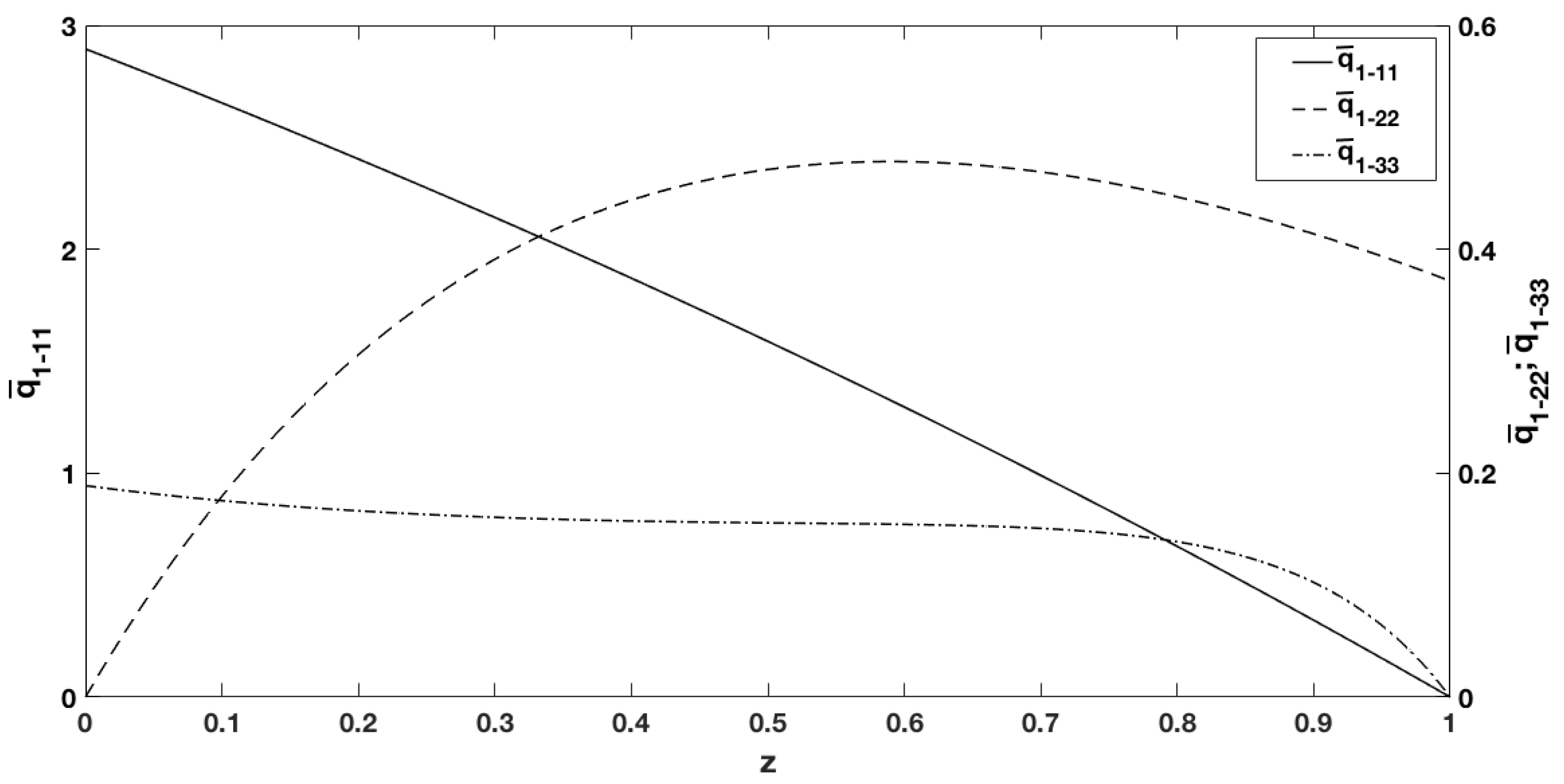
With the assumptions that ${\overline{Q}}_1=\left[\begin{array}{ccc}{\overline{q}}_{1-11}& 0& 0\\ 0& {\overline{q}}_{1-22}& 0\\ 0& 0& {\overline{q}}_{1-33}\end{array}\right]$ and ${\overline{Q}}_2=\left[\begin{array}{cc}{\overline{q}}_{2-11}& 0\\ 0& {\overline{q}}_{2-22}\end{array}\right]$, and by choosing $Q_{11}=\left[\begin{array}{ccc}1& 0& 0\\ 0& 1& 0\\ 0& 0& 1\end{array}\right]$ and $Q_{22}=\left[\begin{array}{cc}{q}_{11}& q_{12}\\ q_{12}& q_{22}\end{array}\right]$, where $q_{11}=q_{22}=1$, one can obtain ${\overline{Q}}_2=\left[\begin{array}{cc}0.25& -0.688\\ -0.688& 1.15\end{array}\right]$ and ${\overline{Q}}_1$, as shown in Figure 4.

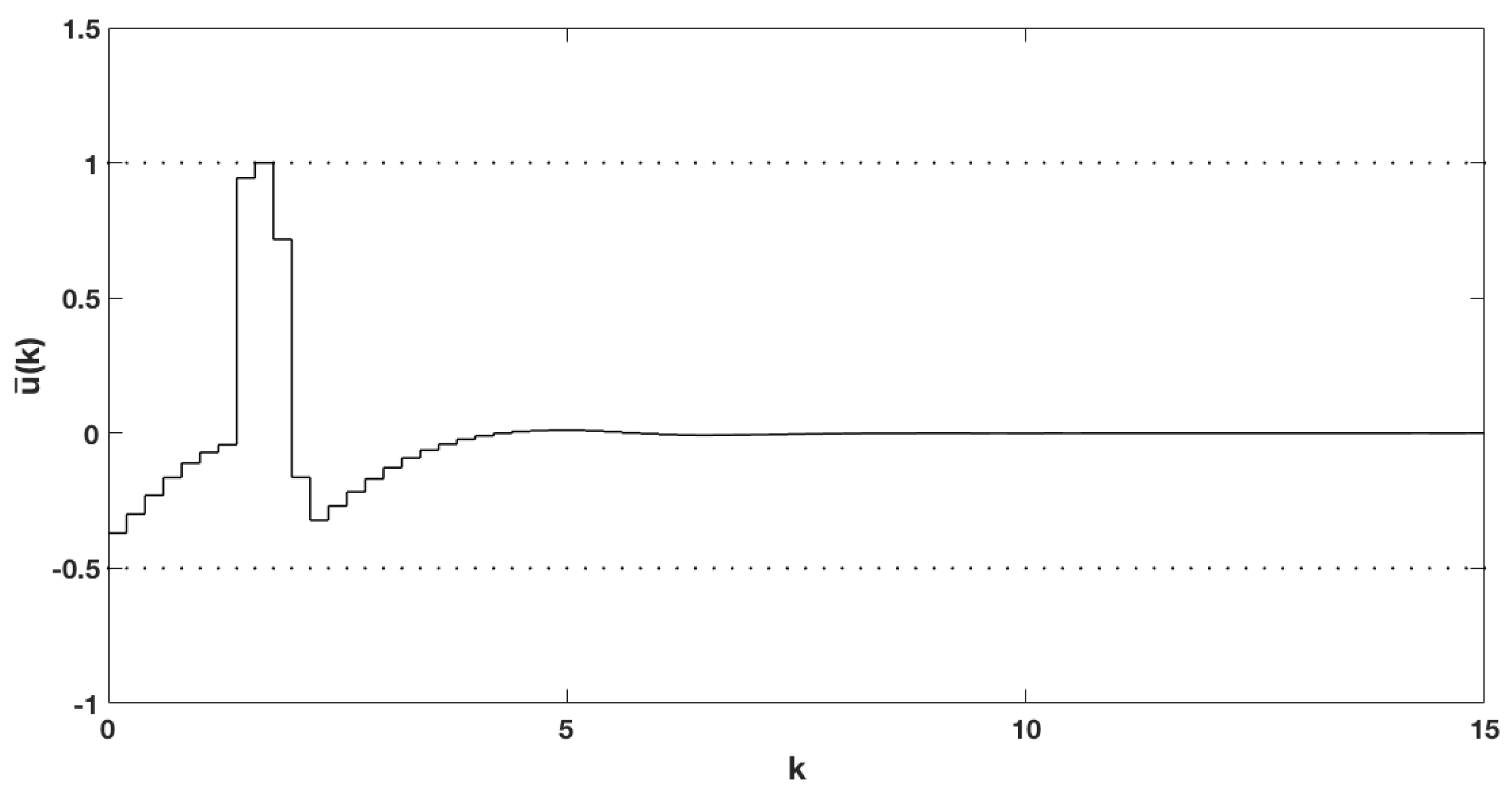
In order to demonstrate the controller performance, the MPC horizon was $N=3$, and $R=0.1$. The input and state constraints were given as $-0.5\le u\left(t\right)\le 1$ and $0\le x_a(h_2,t)\le 0.83$. The initial conditions of the system given by Equation (26) were given as follows:

$$\begin{array}{ccc}\hfill x_a(z,0)& =& a_1(cos\left(\frac{\pi }{2}z\right)+sin\left(\pi z\right)),\hfill \\ \hfill x_{w_d}(z,0)& =& a_2(cos\left(\frac{\pi }{2}z\right)+sin\left(\pi z\right)),\hfill \\ \hfill x_{w_u}(z,0)& =& a_3(cos\left(\frac{\pi }{2}z\right)+sin\left(\pi z\right)).\hfill \end{array}$$

(53)

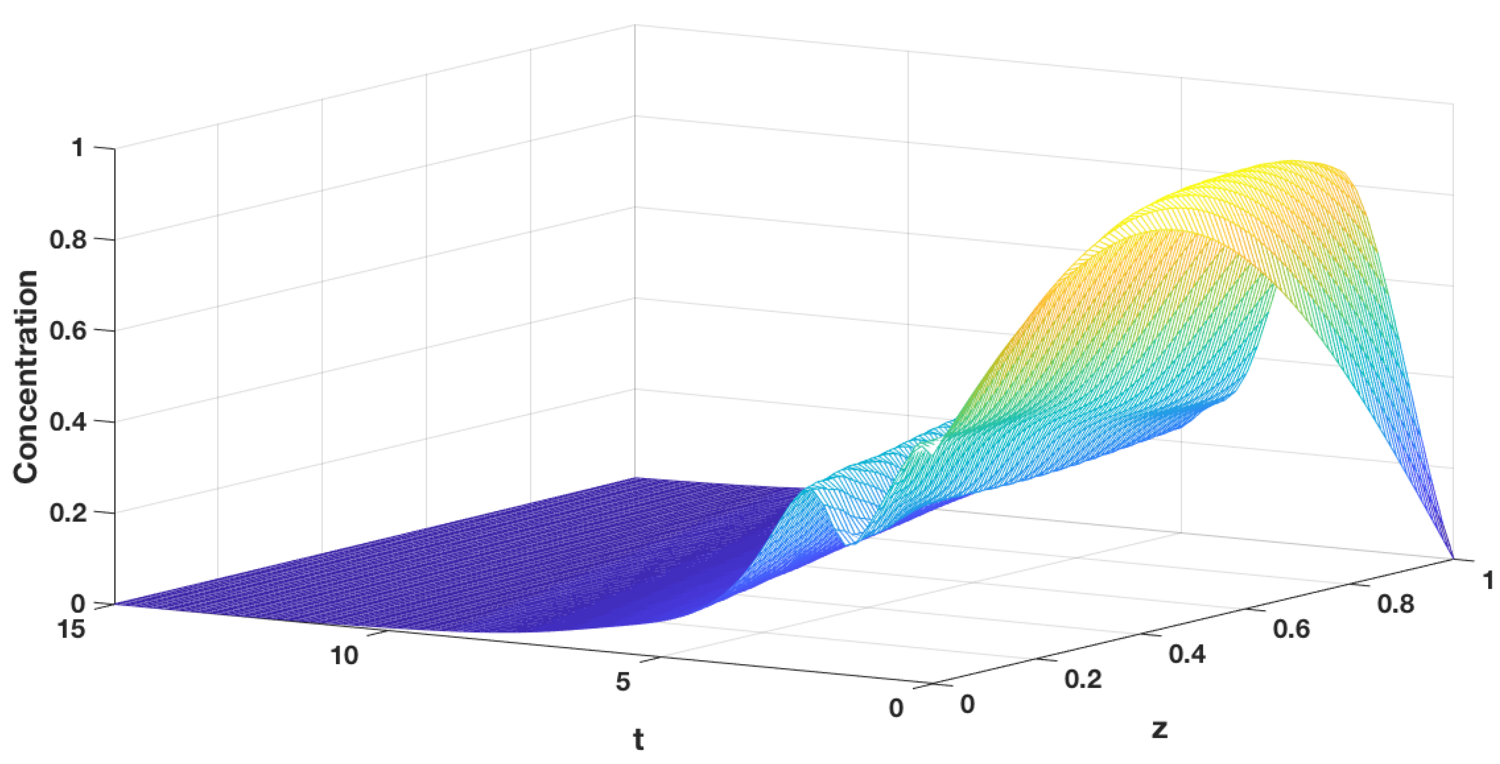
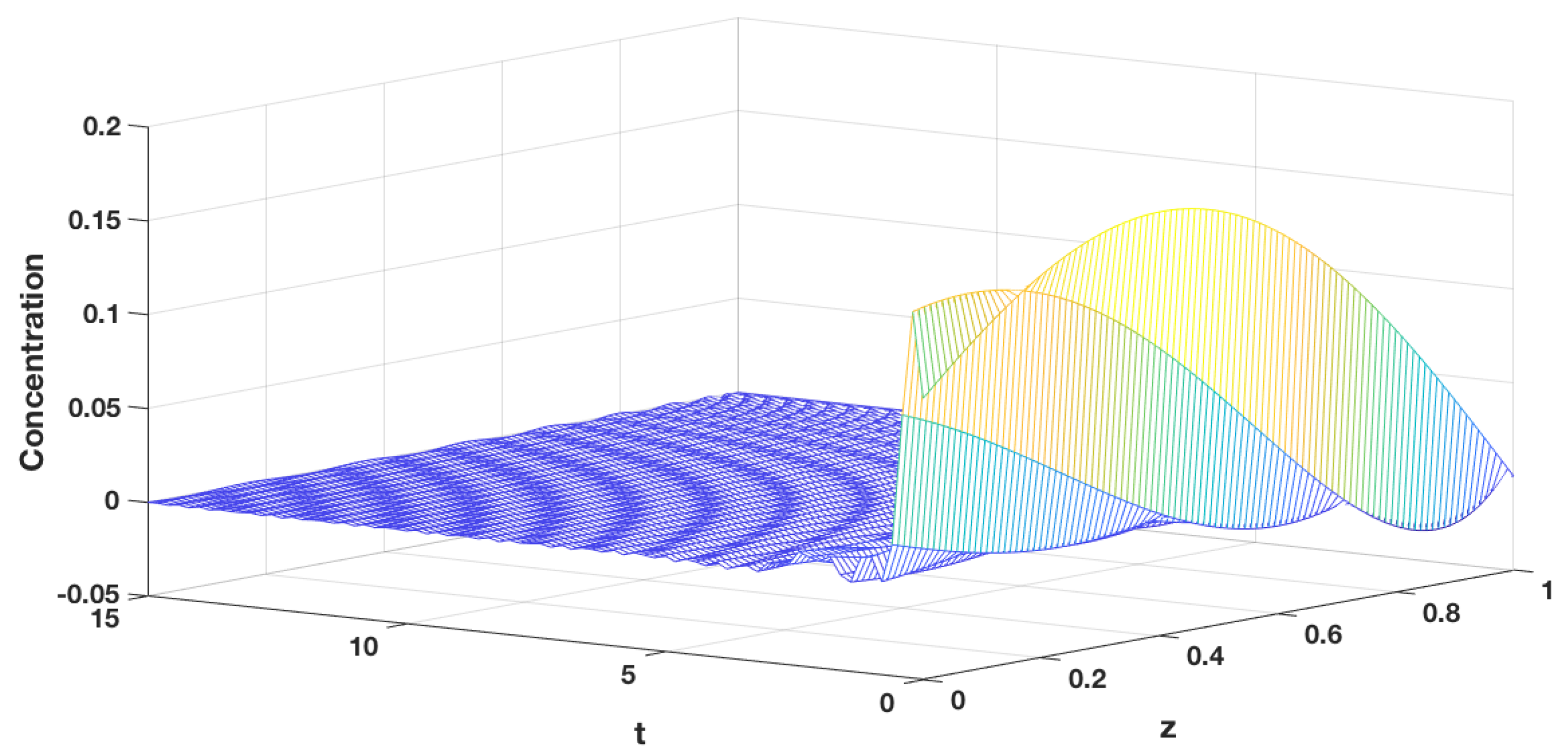
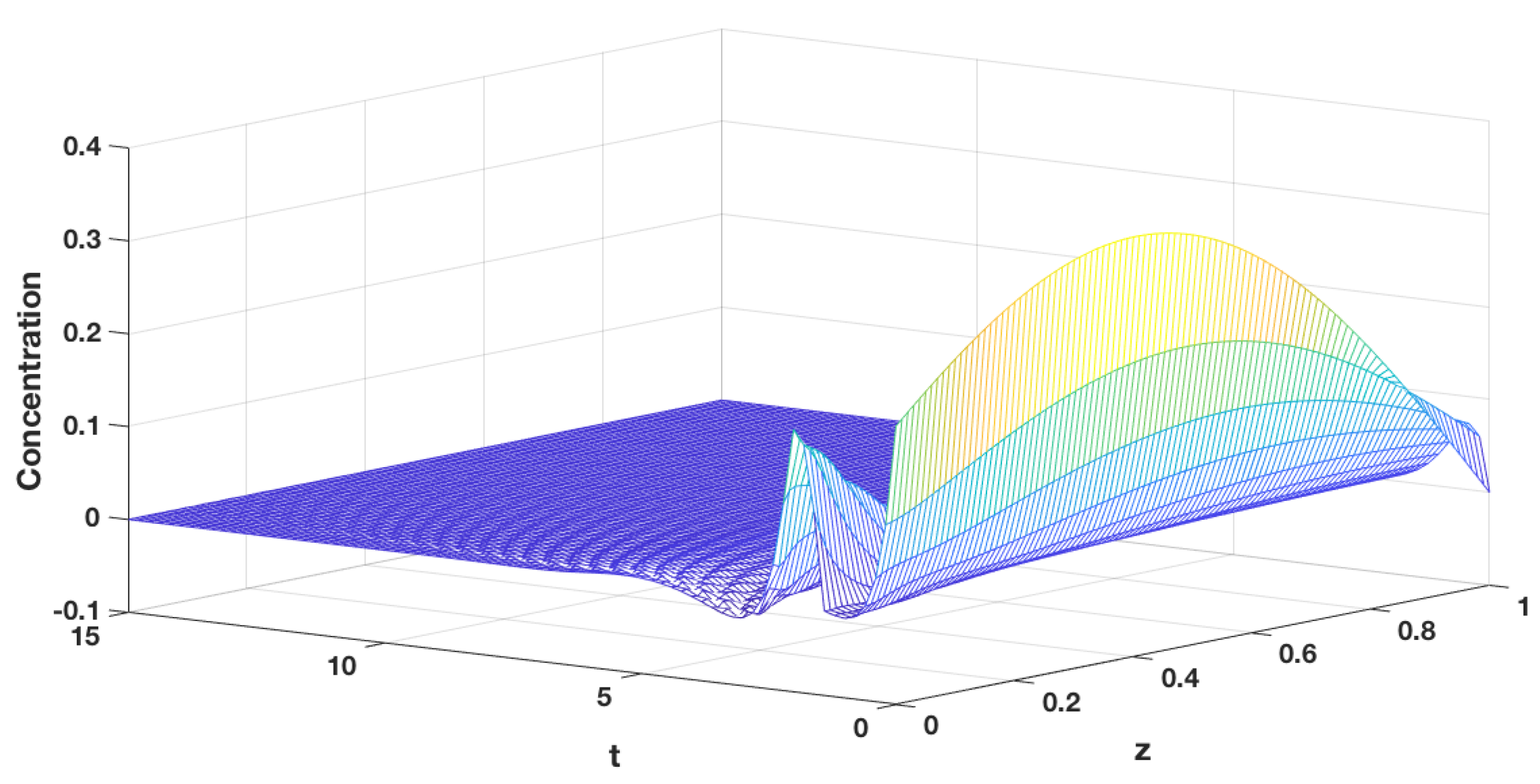
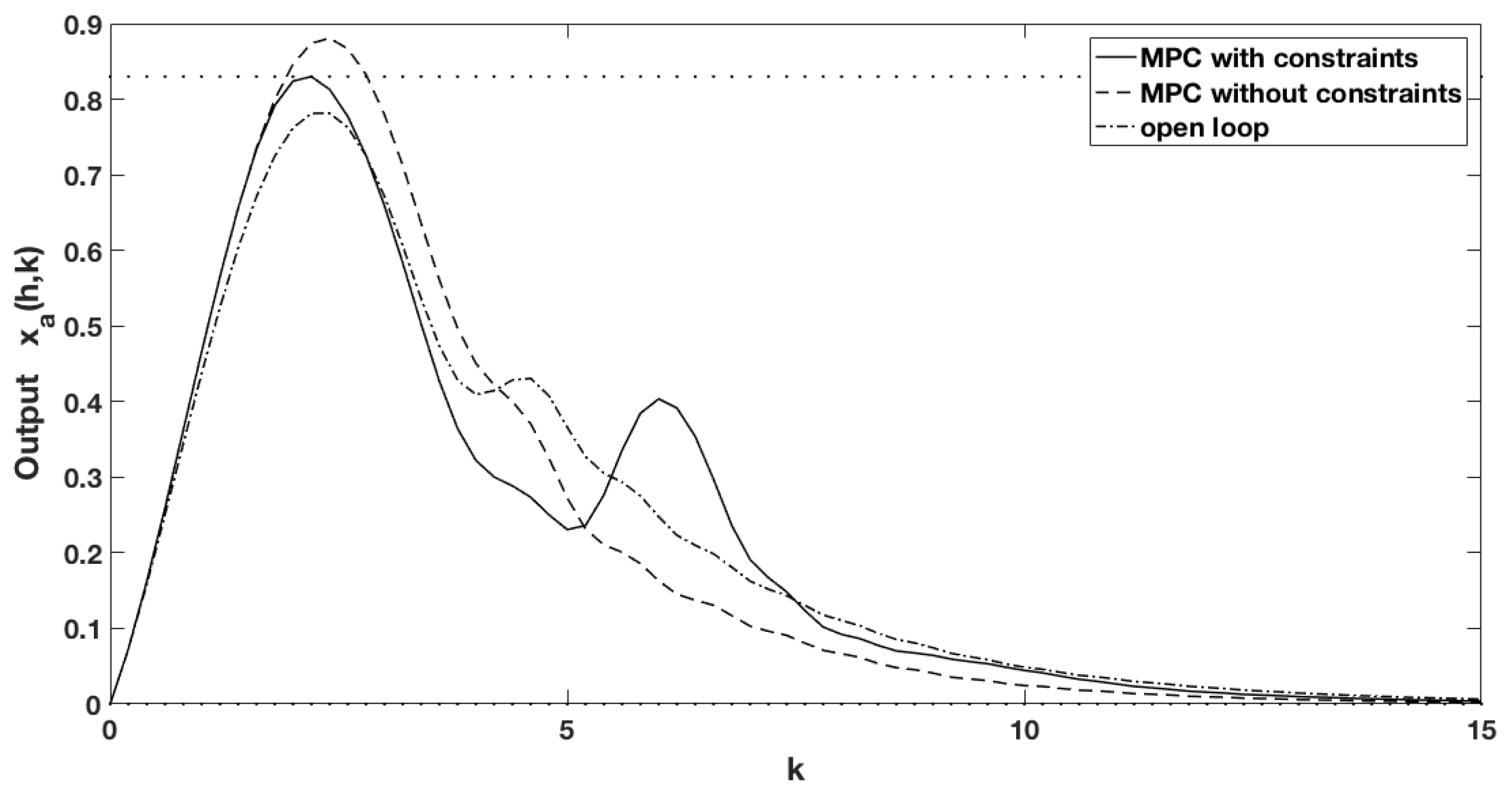
The performance of the proposed model predictive control can be evaluated from Figure 5, Figure 6, Figure 7 and Figure 8, and the corresponding control input is given in Figure 9. From Figure 5, Figure 6 and Figure 7, it can be seen that under the model predictive control, the system reached steady state. Figure 8 compares the output $x_a(h,k)$ evolutions under the model predictive control with state/output constraints to the model predictive control without constraints and using the open-loop system. It is clear from the figure that the application of model predictive control allows the system to reach steady state faster and that the output profile under the model predictive control law satisfies the constraints. It is important to emphasize that the system is stable and that performance under input and state constraints are of interest in this study; however, the extension to the unstable system dynamics case is easily realizable for more general classes of dynamic plants.

5. Conclusions

In conclusion, model predictive control algorithms are developed for the column flotation process that take into account the input and state/output constraints as well as the input disturbance. The underlying model is described by coupled nonlinear heterodirectional hyperbolic transport PDE–ODEs, and the steady-state profiles are utilized in the linearization of a nonlinear system. By using the Cayley–Tustin time discretization method, the continuous infinite-dimensional system is mapped into the discrete infinite-dimensional system without model reduction or spatial discretization. Finally, the performance of the proposed model predictive control development was demonstrated by applying it to the column flotation system, and the simulation results show that the output (the mass concentration of solid minerals with the air phase of froth overflow) is stabilized at the steady state within the constraints’ physical range by adjusting the feed velocity. This optimal control realization improves the column flotation process, enabling it to operate more efficiently.

References

- Finch, J.; Dobby, G. Column Flotation; Pergamon Press: Oxford, UK, 1990. [Google Scholar]
- Kawatra, S.K. Fundamental principles of froth flotation. In SME Mining Engineering Handbook; Society for Mining, Metallurgy, and Exploration: Englewood, IL, USA, 2009; pp. 1517–1531. [Google Scholar]
- Sbárbaro, D.; Del Villar, R. Advanced Control and Supervision of Mineral Processing Plants; Springer Science & Business Media: Berlin/Heidelberg, Germany, 2010. [Google Scholar]
- Mathieu, G. Comparison of flotation column with conventional flotation for concentration of a mo ore. Can. Min. Metall. Bull. 1972, 65, 41–45. [Google Scholar]
- Bergh, L.; Yianatos, J. The long way toward multivariate predictive control of flotation processes. J. Process Control 2011, 21, 226–234. [Google Scholar] [CrossRef]
- McKee, D. Automatic flotation control—A review of 20 years of effort. Miner. Eng. 1991, 4, 653–666. [Google Scholar] [CrossRef]
- Laurila, H.; Karesvuori, J.; Tiili, O. Strategies for instrumentation and control of flotation circuits. Miner. Process. Plant Des. Pract. Control 2002, 2, 2174–2195. [Google Scholar]
- Bouchard, J.; Desbiens, A.; del Villar, R.; Nunez, E. Column flotation simulation and control: An overview. Miner. Eng. 2009, 22, 519–529. [Google Scholar] [CrossRef]
- Bu, X.; Xie, G.; Peng, Y.; Chen, Y. Kinetic modeling and optimization of flotation process in a cyclonic microbubble flotation column using composite central design methodology. Int. J. Miner. Process. 2016, 157, 175–183. [Google Scholar] [CrossRef]
- Mavros, P.; Matis, K.A. Innovations in Flotation Technology; Springer Science & Business Media: Berlin/ Heidelberg, Germany, 2013; Volume 208. [Google Scholar]
- Del Villar, R.; Grégoire, M.; Pomerleau, A. Automatic control of a laboratory flotation column. Miner. Eng. 1999, 12, 291–308. [Google Scholar] [CrossRef]
- Persechini, M.A.M.; Peres, A.E.C.; Jota, F.G. Control strategy for a column flotation process. Control Eng. Pract. 2004, 12, 963–976. [Google Scholar] [CrossRef]
- Bergh, L.; Yianatos, J.; Leiva, C. Fuzzy supervisory control of flotation columns. Miner. Eng. 1998, 11, 739–748. [Google Scholar] [CrossRef]
- Bergh, L.; Yianatos, J.; Acuna, C.; Perez, H.; Lopez, F. Supervisory control at Salvador flotation columns. Miner. Eng. 1999, 12, 733–744. [Google Scholar] [CrossRef]
- Mohanty, S. Artificial neural network based system identification and model predictive control of a flotation column. J. Process Control 2009, 19, 991–999. [Google Scholar] [CrossRef]
- Maldonado, M.; Desbiens, A.; Del Villar, R. Potential use of model predictive control for optimizing the column flotation process. Int. J. Miner. Process. 2009, 93, 26–33. [Google Scholar] [CrossRef]
- Mayne, D.Q.; Rawlings, J.B.; Rao, C.V.; Scokaert, P.O. Constrained model predictive control: Stability and optimality. Automatica 2000, 36, 789–814. [Google Scholar] [CrossRef]
- Malinen, J. Tustin’s method for final state approximation of conservative dynamical systems. IFAC Proc. Vol. 2011, 44, 4564–4569. [Google Scholar] [CrossRef]
- Havu, V.; Malinen, J. Laplace and Cayley transforms—An approximation point of view. In Proceedings of the 44th IEEE Conference on Decision and Control, 2005 and 2005 European Control Conference ( CDC-ECC’05), Seville, Spain, 15 December 2005; pp. 5971–5976. [Google Scholar]
- Havu, V.; Malinen, J. The Cayley transform as a time discretization scheme. Numer. Funct. Anal. Opt. 2007, 28, 825–851. [Google Scholar] [CrossRef]
- Xu, Q.; Dubljevic, S. Linear model predictive control for transport-reaction processes. AIChE J. 2017, 63, 2644–2659. [Google Scholar] [CrossRef]
- Dobby, G.; Finch, J. Mixing characteristics of industrial flotation columns. Chem. Eng. Sci. 1985, 40, 1061–1068. [Google Scholar] [CrossRef]
- Yianatos, J.; Finch, J.; Laplante, A. Cleaning action in column flotation froths. Trans. Inst. Min. Metall. Sect. C-Miner. Process. Extract. Metall. 1987, 96, C199–C205. [Google Scholar]
- Franklin, G.F.; Powell, J.D.; Workman, M.L. Digital Control of Dynamic Systems; Addison-Wesley: Menlo Park, CA, USA, 1998; Volume 3. [Google Scholar]
- Xu, Q.; Dubljevic, S. Modelling and control of solar thermal system with borehole seasonal storage. Renew. Energy 2017, 100, 114–128. [Google Scholar] [CrossRef]
- Muske, K.R.; Rawlings, J.B. Model predictive control with linear models. AIChE J. 1993, 39, 262–287. [Google Scholar] [CrossRef]
Figure 1.
Schematic representation of a flotation column.
Figure 2.
Steady-state profile of mineral.
Figure 3.
Schematic representation of coupled partial differential equations (PDEs) and ordinary differential equations (ODEs) system connected through boundary.
Figure 4.
obtained by solving Equation (52).
Figure 5.
Profile of concentration for mineral particles with air phase under model predictive control law Equations (48) and (49).
Figure 6.
Profile of concentration for mineral particles with downward water phase under model predictive control law Equations (48) and (49).
Figure 7.
Profile of concentration for mineral particles with upward water phase under model predictive control law Equations (48) and (49).
Figure 8.
Profile of the state (output) under model predictive control law Equations (48) and (49) (dash-dotted line) without constraints (dashed line), and the profile of an open-loop system (dash-dotted line), as well as state/output constraints (dotted line).
Figure 9.
Input profile obtained by model predictive control law Equations (48) and (49) (solid line); input constraints are given by dotted line.