Divisibility Patterns within Pascal Divisibility Networks
by
 , and
, and
Pedro A. Solares-Hernández
1,2,3, 
Fernando A. Manzano
1,2,3 ,
,
Francisco J. Pérez-Benito
1,4 and
J. Alberto Conejero
1,*
1
Instituto Universitario de Matemática Pura y Aplicada, Universitat Politècnica de València, 46022 València, Spain
2
Departamento de Estadística, Universidad APEC, Santo Domingo 10203, Dominican Republic
3
Departamento de Ingeniería, Universidad APEC, Santo Domingo 10203, Dominican Republic
4
Instituto de Tecnología Informática (ITACA), Universitat Politècnica de València, 91354 València, Spain
*
Author to whom correspondence should be addressed.
Mathematics 2020, 8(2), 254; https://doi.org/10.3390/math8020254
Submission received: 31 December 2019
/
Revised: 3 February 2020
/
Accepted: 7 February 2020
/
Published: 14 February 2020
(This article belongs to the Section Network Science)
Abstract
:The Pascal triangle is so simple and rich that it has always attracted the interest of professional and amateur mathematicians. Their coefficients satisfy a myriad of properties. Inspired by the work of Shekatkar et al., we study the divisibility patterns within the elements of the Pascal triangle, through its decomposition into Pascal’s matrices, from the perspective of network science. Applying Kolmogorov–Smirnov test, we determine that the degree distribution of the resulting network follows a power-law distribution. We also study degrees, global and local clustering coefficients, stretching graph, averaged path length and the mixing assortative.
1. Introduction
Number theory has been one of the most studied fields of mathematics for centuries. In contrast, network science has emerged as a discipline in the last twenty years. Nevertheless, networks have attracted the interest of many researchers due to their multiple applications to different disciplines, such as biology, telecommunications, social and environmental sciences, as well as systems medicine.
Besides, some networks have emerged from mathematical concepts, such as the divisibility network. This was firstly studied by Zhou et al. in [1]. Here, nodes represent natural numbers and two nodes are connected by a directed edge if n divides m, denoted by . These authors noticed that this network has a large clustering coefficient of approximately 0.34, which is insensitive to the network size. Besides, they showed that: (i) The average distance between a pair of nodes is upper bounded, in contrast to small-world networks, (ii) it posses a hierarchical architecture, and (iii) the degree distribution follows a power-law.
A divisibility network can also be considered as a non-directed one if we connect a pair of nodes if either or . Shekatkar et al. [2] studied it using the framework of a growing complex network. Among other properties, they showed that it is scale-free but has a non-stationary degree distribution, reporting a stretching similarity pattern, and showing how this pattern evolves with the size of the network. Related to divisibility networks, Yan et al. [3] showed that every layer in a multiplex congruence network is a sparse and heterogeneous subnetwork satisfying the scale-free property, providing an insight into the simultaneous congruences problem through the graphical solutions provided there.
All these results have inspired us to look for other ways of consider the divisibility network through a different growing network procedure. Due to the abundance of beautiful and unpredictable properties hidden in the Pascal Triangle (PT), we have studied the non-directed divisibility following a similar approach as Shekatkar et al. did. For this purpose, we have considered squared Pascal symmetric matrices as a covering of growing finite subsets of the PT. These matrices were firstly analyzed by Brawer and Pirovino [4]. We will denote by the Pascal square matrix of order n, that is obtained when taking the square with two orthogonal sides given by the first n ones of both sides of the PT. As an example, we have indicated in bold font the Pascal matrix in (1). From we construct a divisibility network whose nodes are .
Pascal matrices present some beautiful properties. As an example, we mention the decomposition of the Pascal matrices proposed by Edelman and Strang [5] who showed how to decompose any Pascal matrix of order n, into the product of two matrices , which is a lower triangular matrix, and , which is an upper triangular matrix, such that, , for every .
For any given number , there is some such that for all . With this in mind, we will study the divisibility networks provided by these matrices. On the one hand, using these matrices, we can cover all the natural numbers through a growing family of subnetworks. On the other hand, the numbers in these matrices are not consecutive, and when sequentially ordered, we can find big gaps between some of them. This suggests us to study whether the scale-free degree distribution holds and other network properties are still satisfied as to the ones shown in [2].
In particular, we have considered the evolution of several network measures along with the size of Pascal matrices, such as the average degree , the histogram of the connectivity degree distribution; the local and global clustering coefficients and , the assortativity index r; and the average path length . We will recall the definition of these notions in the next section.
The degree distribution is studied in Section 2.1, where we show that it is scale-free. We also study an example of how to compute the fitting parameters. In order to study the structure of this network, we have studied how the clustering evolves with the size of the network. The local and global clustering coefficients are presented in Section 2.2 and Section 2.3. The tendency of nodes to connect to nodes of similar degree is analyzed through the assortative coefficient in Section 2.4, and how nodes are separated respect to the others through the average path length, see Section 2.5.
2. Network Analysis
For any arbitrary , we consider the divisibility network , associated to the Pascal matrix of order n. This network has as its set of nodes and as its set of edges. We point out that we exclude the number 1 of since it will be linked with any other number, which does not provide useful information for studying the evolution of the network properties of these matrices.
We denote card by , with , and card by . Once fixed the set of nodes with the non-repeated elements of , we recall that an arbitrary pair of elements are linked by an edge if, and only if, or . Figure 1a,b are generated from matrices and .
2.1. Degree Distribution
Given the sequence of nodes from a network , with , we first analyze the evolution of the degree distribution , where is the number of coefficients with degree k in , along with n. First, we check if the scale-free property holds, which will result into the existence of many nodes with only a few edges and a few nodes with a large number of edges, that are called hubs, see [6,9].
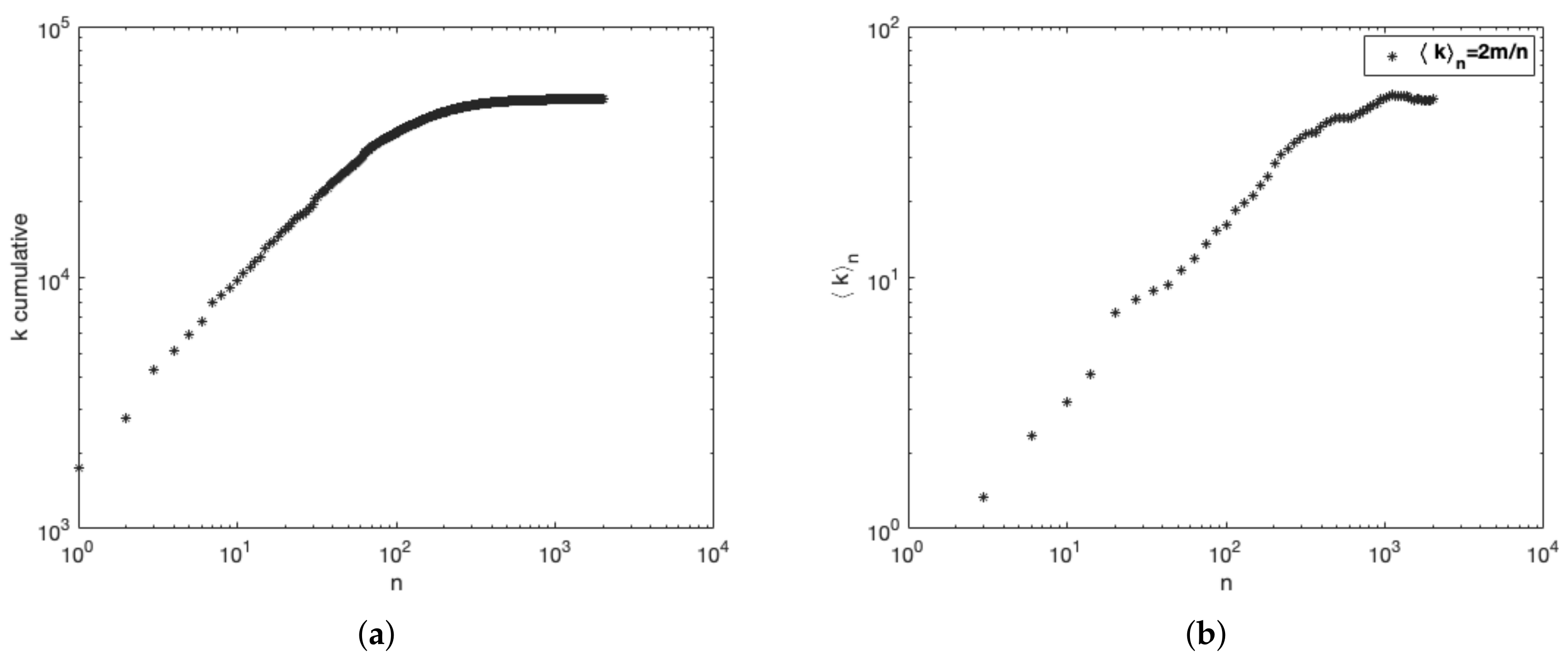
In Figure 2, we illustrate the asymptotic growth of the cumulative and the averaged cumulative degree distributions for the network , that has a total of 2001 nodes and 51147 edges. The nodes are indexed in increasing order respect to the term of that they represent. We appreciate how both measures tend to stabilize when adding the last nodes of each network.
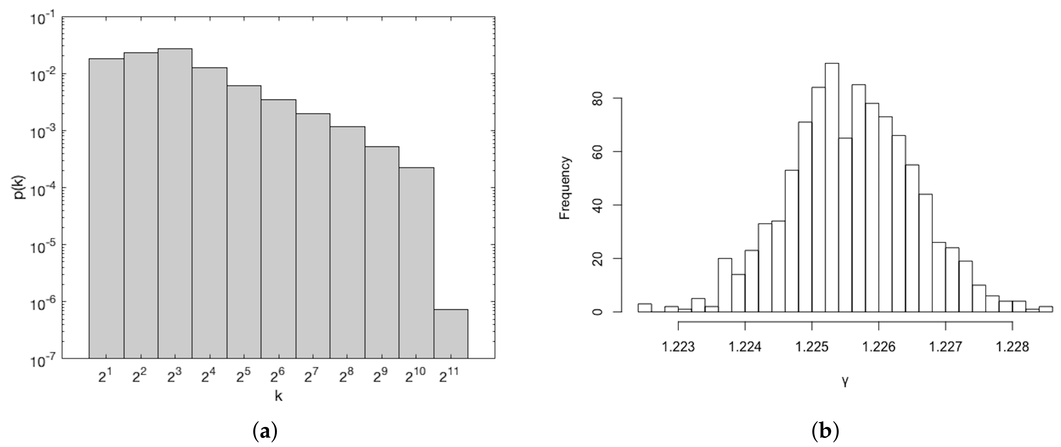
Applying the Maximum Likelihood method [2,10], we confirm that the divisibility network of Pascal matrices satisfies a scale-free law. This means that the network degree distribution follows, at least asymptotically, a power-law of the form for all . We recall that when the power-law governs a process, this usually occurs from what we determinate the “minimum value” , which is exactly the point where one can start to observe the fall of the heavy tail. In Figure 3a, we represent again the degree distribution for with logarithmic binning in the degree values.
We characterize the power-law of the degree distribution of through bootstrapping, using 1000 iterations of bootstrapping. The obtained fitting parameters were and . In Figure 2a, we plot the histogram of the values obtained for the parameter. For , the Kolmogorov–Smirnov coefficient was , see Figure 3b, which shows the goodness of the estimation. It is worth to mention that network with similar degree distributions could have a different inner structure, see [11].
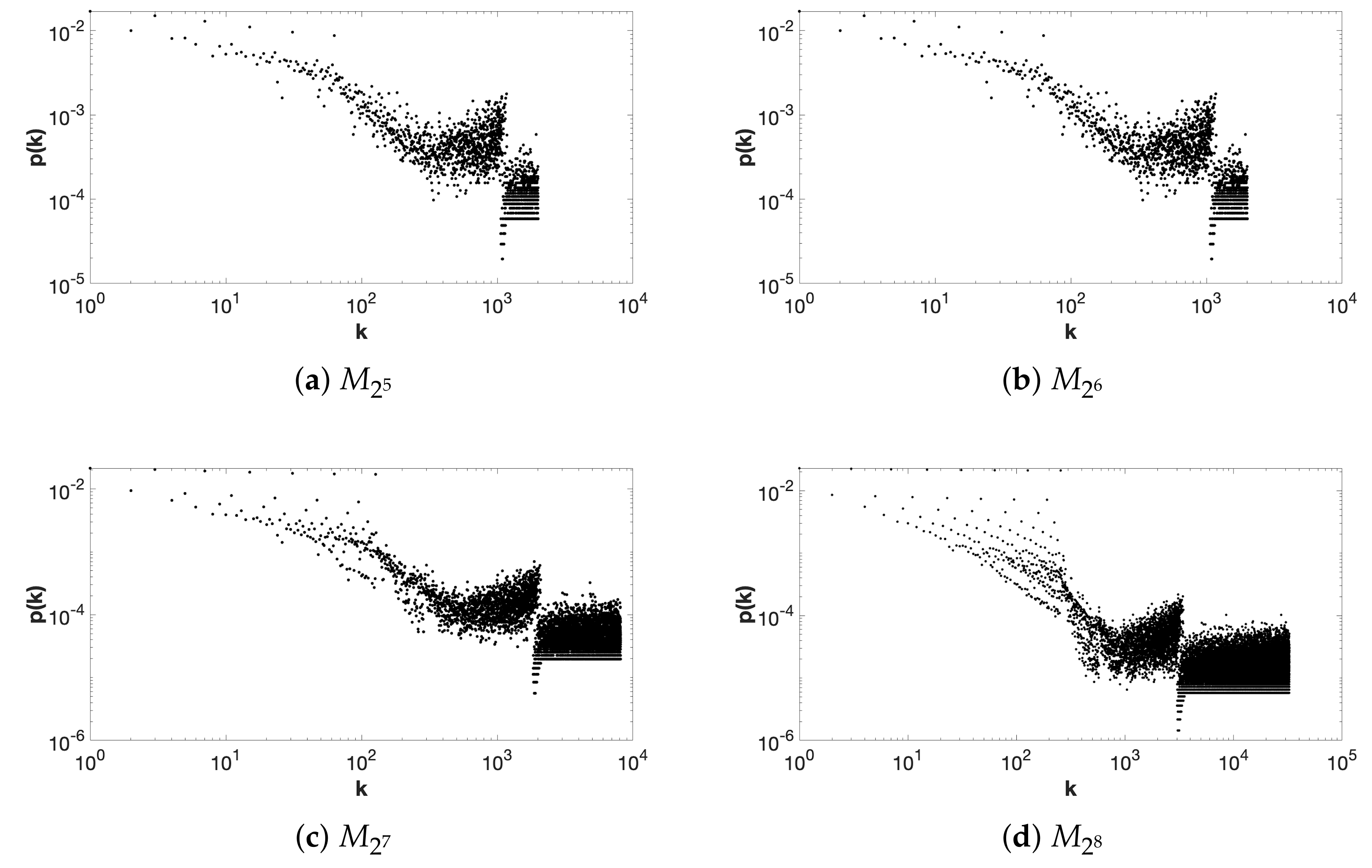
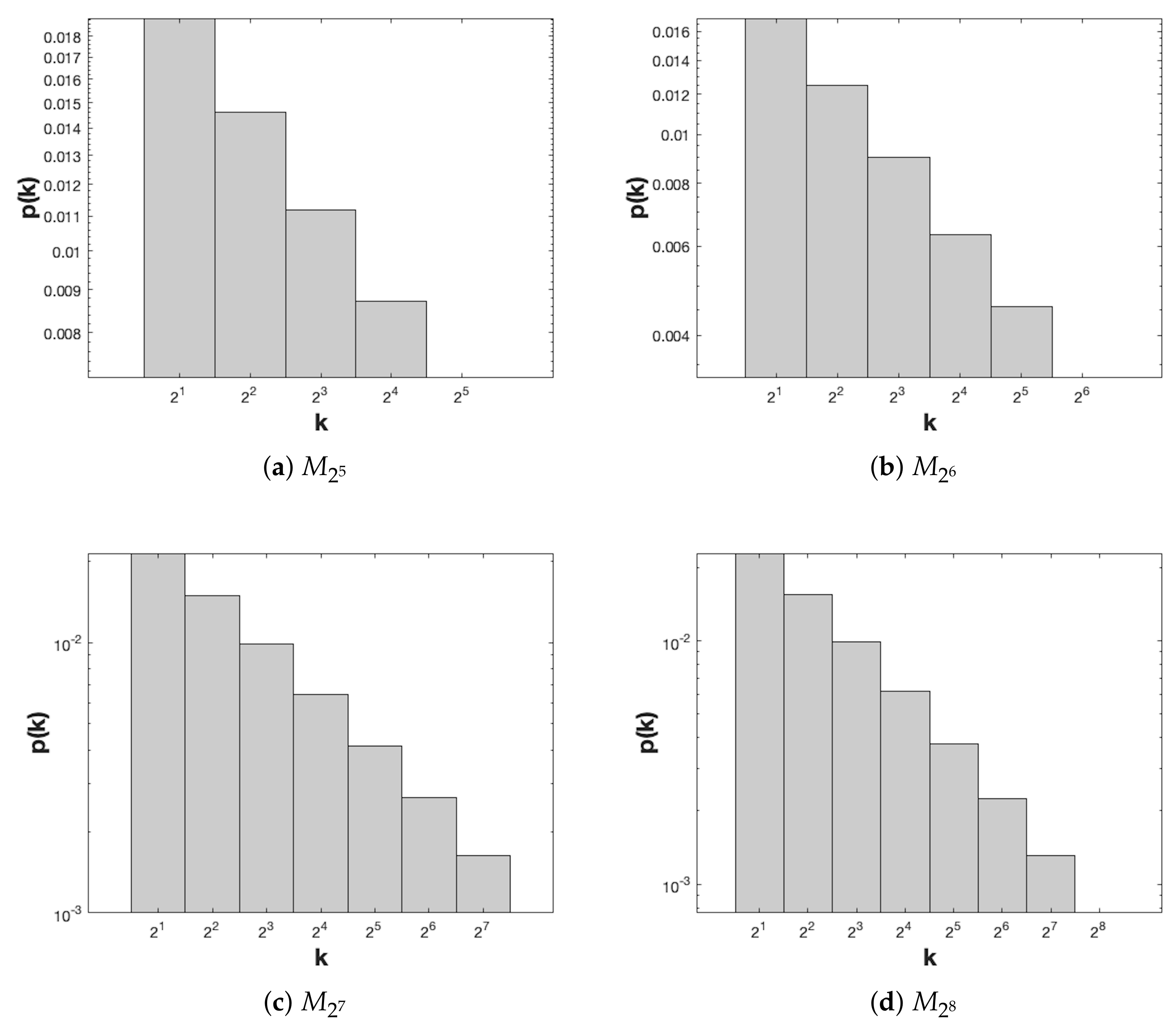
We also show the degree distributions of , , and in Figure 4. We observe a high concentration of nodes (plateau) in the region of high values of the degree. This suggests a bias in the linear model fitting due to the comparatively large number of nodes with low degrees respect to the fewer number of nodes with large degrees [6,12].
In order to correct the non-uniform sampling seen with the linear binning, we show these degrees distributions with logarithmic binning again, see Figure 5.
As n grows, the coefficient of the power-law fitting decreases. Increasing the number of nodes of the network does not guarantee a better fit of the linear model. It is worth to mention that these indicators do not fully reflect the network robustness due to the inherent bias of the particular sampling process, see for instance [13].
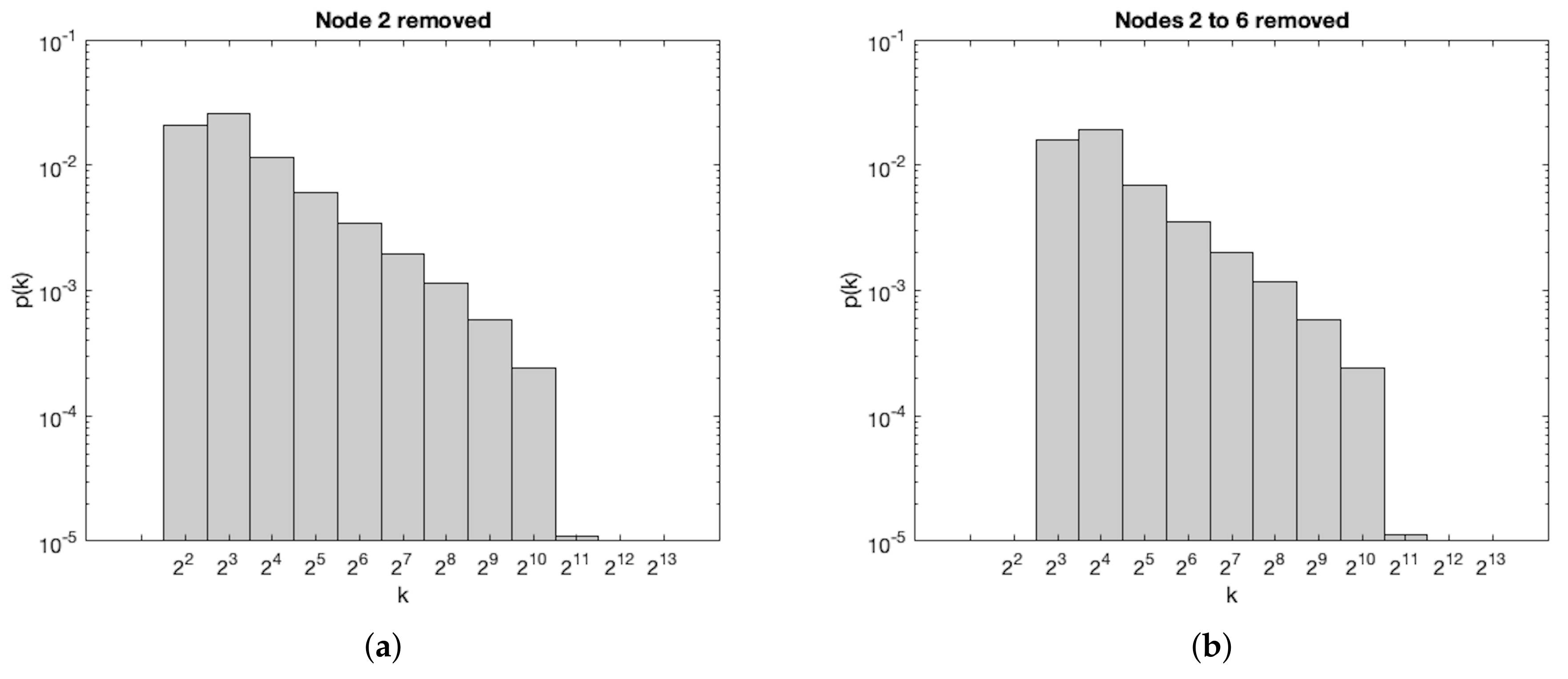
We also have wondered how important is the role of the lowest numbers, which have the highest degrees, in determining the scale-free nature of the network. In this line, we have removed the hubs corresponding to nodes associated with numbers 2 to 6. These new degree distributions also follow a power-law, as we can see in Figure 6.
2.2. Local Clustering Coefficient
Many scale-free networks also display a high degree of clustering. This is the result of a hierarchical organization in which small groups of nodes organize into increasingly larger ones while preserving the scale-free property [14].
Since all the natural numbers appear along the first row/column of Pascal matrices, and the rest of their elements are composite numbers, there will be many connections from the first elements to the second ones. Besides, as numbers in the inner columns/rows of the matrices grow pretty fast, there will be fewer edges among them. Therefore, we have analyzed how clustered the network is. The main two measures for analyzing the clustering are the local and the global clustering coefficients. The global version provides an indicator of the clustering in the network, whereas the local one gives an indicator of the connection between the adjacent nodes to a given one.
We recall that given and a node with degree , we denote by the set of nodes adjacent to . Then, the local clustering coefficient is the number of pairs of adjacent nodes to that are connected between them by an edge, divided by the number of admissible neighbor pairs of [8,15,16] that is:
2.3. Global Clustering Coefficient
The global clustering coefficient is based on ordered triplets of connected nodes, that can be linked by 2 (open triplet) or 3 edges (closed triplet). With this, a triangle graph has 3 closed triplets: That is, a triangle ABC has 3 triplets associated to it: ABC, BCA, and CAB. With this, the global clustering coefficient can be computed as
As we can see in Figure 9 the global clustering coefficients decreases when the size of grows, approaching 0 for high values of n, which represents that the networks become more and more sparse when increasing its size n.
2.4. Assortative Coefficient
The assortativity coefficient r the correlation coefficient of the degrees of adjacent nodes. It shows the preference of nodes to connect with other nodes of comparable degree [8,17].
Given a network , it is defined as follows:
where is the degree of , is the element of the adjacency matrix associated to the eventual connection between and , is the total of links in the network, and is the Kronecker delta. However, determining the assortativity from (4) supposes a high computational cost, and therefore it is suggested to approximate the assortativity by means of the next expression ([8], Section 10.7):
where we have introduced for referring to all unordered pairs of nodes connected by an edge and is the total number of nodes of a network .
Assortativity coefficient presents values ranging from to 1. If , we called the network to be fully assortative. In case of the network is said to be not assortative, while if , the network is called disassortative [15,17,18]. The divisibility networks approaches to be disassortative as long as n increases, see Figure 9, which reflects that nodes that have a high degree tend to connect with low-grade nodes.
2.5. Average Path Length
The network average path length, denoted by is the averaged distance between all pairs of nodes. For each pair, the distance between them is given by the shortest path connecting them. Clearly, if two nodes belong to different connected components, the distance will be ∞. For computing the average path length we have excluded pairs of nodes belonging to different connected components.
We can see that, if connected, the averaged path length is short. In Figure 9, we show it for several networks. It increases with the size of the network, but even for it is 2.05. This means that the biggest connected component is closed to be a bipartite network.
3. Conclusions
PT and Pascal matrices present multiple properties that have fascinated mathematicians for ages. Here, we have studied them from the perspective of Network Science. We have considered Pascal matrices as a ground for constructing a growing divisibility network. Its structure has been studied, following the approach of [2]. The interest of this choice lies in the fact that PT contains all the natural numbers on each of their sides. The way in which we increasingly construct the divisibility network by taking the Pascal matrices provides a different arrangement of the natural numbers, with gaps between some of them. Nevertheless, the scale-free property for the degree distribution also holds.
Either in [2] or here, both growing networks present similar structures and characteristics to real based networks. This can be noticed when looking at the degree distribution, the global and local clustering coefficients, the assortativity, and the average path length. This work fits within our interest in studying divisibility networks constructed from subsets of the natural numbers, and to see how network measures can help us to describe them and how to find hidden structures and hierarchies [19]. In future works, we will study the divisibility networks provided by other arrangements of the natural numbers, and the divisibility networks of other countable sets of numbers such as the rational numbers in the unit interval [20].
The results concerning the local clustering coefficient are similar to the ones given by [2]. Besides, we have seen that when the size of the network grows, the global clustering coefficient tends to 0, and the divisibility networks approach more and more to being disassortative. Both results agree with the average path length that, despite low, it increases as the network size grows and indicates that the network is close to being bipartite.
Author Contributions
Conceptualization, P.A.S.-H. and J.A.C.; software P.A.S.-H, F.J.P.-B. and F.A.M.; validation and formal analysis, P.A.S.-H. and J.A.C.; writing–original draft preparation, writing–review and editing, P.A.S.-H., F.J.P.-B., F.A.M. and J.A.C. All authors have read and agreed to the published version of the manuscript.
Funding
J.A.C. was funded by MEC grant number MTM2016-75963-P. P.A.S.-H. acknowledges the support of MESCyT-RD and Casa Brugal for his PhD grants.
Conflicts of Interest
The authors declare no conflict of interest. The funding institutions had no role in the design of the study; in the collection, analyses, or interpretation of data; in the writing of the manuscript, or in the decision to publish the results.
References
- Zhou, T.; Wang, B.H.; Hui, P.; Chan, K. Topological properties of integer networks. Phys. A Stat. Mech. Appl. 2006, 367, 613–618. [Google Scholar] [CrossRef] [Green Version]
- Shekatkar, S.M.; Bhagwat, C.; Ambika, G. Divisibility patterns of natural numbers on a complex network. Sci. Rep. 2015, 5, 14280. [Google Scholar] [CrossRef] [PubMed] [Green Version]
- Yan, X.Y.; Wang, W.X.; Chen, G.R.; Shi, D.H. Multiplex congruence network of natural numbers. Sci. Rep. 2016, 6, 23714. [Google Scholar] [CrossRef] [PubMed] [Green Version]
- Brawer, R.; Pirovino, M. The linear algebra of the Pascal matrix. Linear Algebr. Its Appl. 1992, 174, 13–23. [Google Scholar] [CrossRef]
- Edelman, A.; Strang, G. Pascal matrices. Am. Math. Mon. 2004, 111, 189–197. [Google Scholar] [CrossRef]
- Barabási, A.-L. Network Science; Cambridge University Press: Cambridge, UK, 2016. [Google Scholar]
- Estrada, E. The Structure of Complex Networks: Theory and Applications; Oxford University Press: Oxford, UK, 2012. [Google Scholar]
- Newman, M. Networks; Oxford University Press: Oxford, UK, 2018. [Google Scholar]
- Barabási, A.L.; Albert, R. Emergence of scaling in random networks. Science 1999, 286, 509–512. [Google Scholar] [CrossRef] [PubMed] [Green Version]
- Clauset, A.; Shalizi, C.; Newman, M. Power-law distributions in empirical data. SIAM Rev. 2009, 51, 661–703. [Google Scholar] [CrossRef] [Green Version]
- Shang, Y. Distinct clusterings and characteristic path lengths in dynamic small-world networks with identical limit degree distribution. J. Stat. Phys. 2012, 149, 505–518. [Google Scholar] [CrossRef]
- Gillespie, C. Fitting heavy tailed distributions: The poweRlaw Package. J. Stat. Softw. 2015, 64, 1–16. [Google Scholar] [CrossRef]
- Shang, Y. Subgraph robustness of complex networks under attacks. IEEE Trans. Syst. Man Cybern. Syst. 2017, 49, 821–832. [Google Scholar] [CrossRef]
- Ravasz, E.; Barabási, A. Hierarchical organization in complex networks. Phys. Rev. 2003, 67, 026112. [Google Scholar] [CrossRef] [PubMed] [Green Version]
- Dorogovtsev, S.; Mendes, J. Evolution of networks. Adv. Phys. 2002, 51, 1079–1187. [Google Scholar] [CrossRef] [Green Version]
- Newman, M. The structure and function of complex networks. SIAM Rev. 2003, 45, 167–256. [Google Scholar] [CrossRef] [Green Version]
- Newman, M. Mixing patterns in networks. Phys. Rev. 2003, 67, 026126. [Google Scholar] [CrossRef] [PubMed] [Green Version]
- Newman, M. Assortative mixing in networks. Phys. Rev. 2002, 89, 208701. [Google Scholar] [CrossRef] [PubMed] [Green Version]
- Bunimovich, L.; Smith, D.; Webb, B. Finding hidden structures, hierarchies, and cores in networks via isospectral reduction. Appl. Math. Nonlinear Sci. 2019, 4, 225–248. [Google Scholar] [CrossRef] [Green Version]
- Hernández-Solares, P.; Conejero, J.A. Divisibility patterns of the rational numbers on the interval on a complex network. Preprint 2020. [Google Scholar]
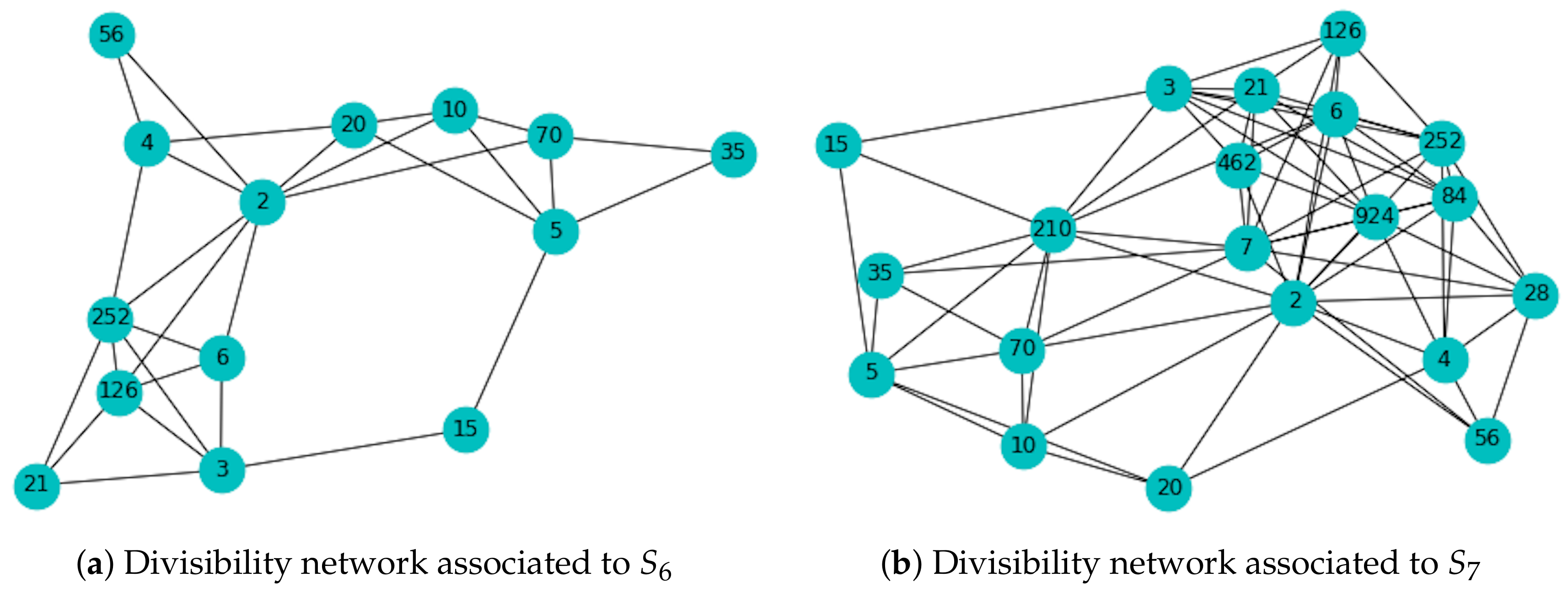
Figure 1.
Examples of divisibility networks obtained from Pascal matrices and . From , we have that the network has 14 nodes and 29 edges, see Figure 1a, and from we have that has 20 nodes and 72 edges, see Figure 1b.

Figure 2.
Cumulative degree and average degree distributions for the network . Figure 2a shows the cumulative degree as the coefficients of grow in value. Figure 2b plots the evolution of the average degree when the coefficients of are progressively added. For the average degree is .

Figure 3.
In Figure 3a, the sizes of the bins are equal to successive positive powers of 2, and the count in each bin is normalized dividing by the bin width, like in ([2], Figure 2). In Figure 3b, we characterize the uncertainty in the parameter fitting to a power law using 1000 bootstraps for .

Figure 4.
Representation of the degree distribution for , and .

Figure 5.
Representation of the degree distribution for , and , with logarithmic bining.

Figure 6.
Degree distributions of the Pascal network with logarithmic bining. In Figure 6a we have removed node 2 and in Figure 6b we have removed nodes 2 to 6.

Figure 7.
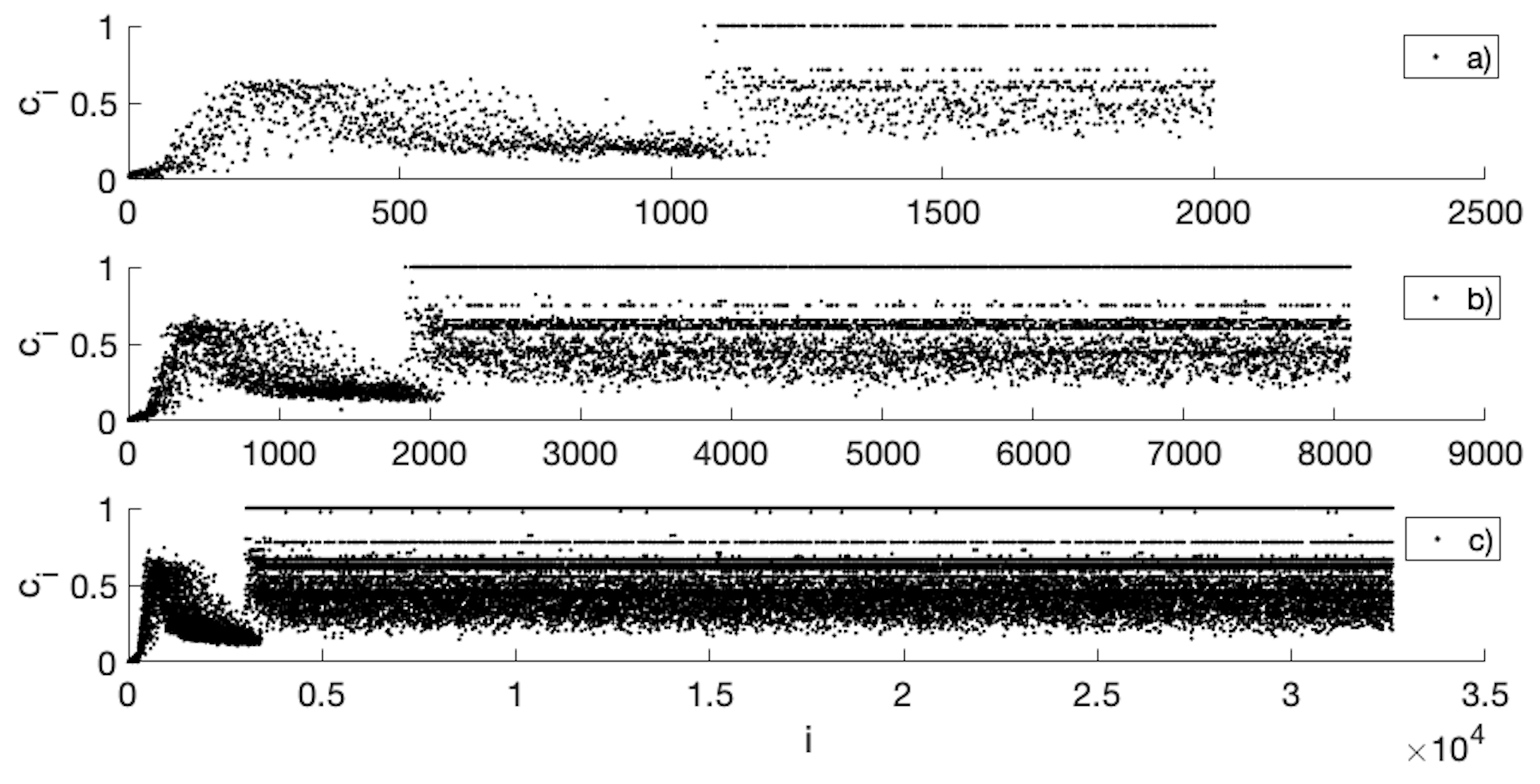
Local clustering coefficient in terms of the node index for different network sizes: (a) , (b) , (c) . Nodes are indexed in increasing order of the number to which they are associated. This graph shows a stretch of similarity due to the divisibility between the coefficients of the Pascal matrix. The stretch is the same, regardless of the size of the network, as was shown in [2].
Figure 7.
Local clustering coefficient in terms of the node index for different network sizes: (a) , (b) , (c) . Nodes are indexed in increasing order of the number to which they are associated. This graph shows a stretch of similarity due to the divisibility between the coefficients of the Pascal matrix. The stretch is the same, regardless of the size of the network, as was shown in [2].

Figure 8.
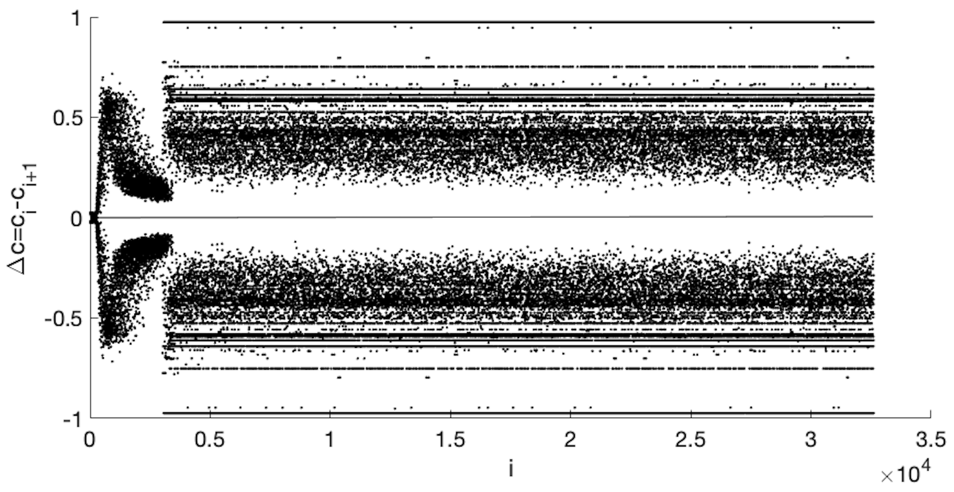
Behavior of the evolution of the difference between the clustering coefficient and the clustering coefficient .
Figure 8.
Behavior of the evolution of the difference between the clustering coefficient and the clustering coefficient .

Figure 9.
Evolution of the global clustering, assortativity, and average path length for , and .

© 2020 by the authors. Licensee MDPI, Basel, Switzerland. This article is an open access article distributed under the terms and conditions of the Creative Commons Attribution (CC BY) license (http://creativecommons.org/licenses/by/4.0/).
Share and Cite
MDPI and ACS Style
Solares-Hernández, P.A.; Manzano, F.A.; Pérez-Benito, F.J.; Conejero, J.A. Divisibility Patterns within Pascal Divisibility Networks. Mathematics 2020, 8, 254. https://doi.org/10.3390/math8020254
AMA Style
Solares-Hernández PA, Manzano FA, Pérez-Benito FJ, Conejero JA. Divisibility Patterns within Pascal Divisibility Networks. Mathematics. 2020; 8(2):254. https://doi.org/10.3390/math8020254
Chicago/Turabian StyleSolares-Hernández, Pedro A., Fernando A. Manzano, Francisco J. Pérez-Benito, and J. Alberto Conejero. 2020. "Divisibility Patterns within Pascal Divisibility Networks" Mathematics 8, no. 2: 254. https://doi.org/10.3390/math8020254
Note that from the first issue of 2016, this journal uses article numbers instead of page numbers. See further details here.