The Effect of a Linear Tuning between the Antigenic Stimulations of CD4⁺ T Cells and CD4⁺ Tregs

Abstract

We study the equilibria of an Ordinary Differencial Equation (ODE) system where CD4${}^{+}$ effector or helper T cells and Regulatory T cells (Tregs) are present. T cells trigger an immune response in the presence of their specific antigen. Regulatory T cells (Tregs) play a role in limiting auto-immune diseases due to their immune-suppressive ability. Here, we present explicit exact formulas that give the relationship between the concentration of T cells, the concentration of Tregs, and the antigenic stimulation of T cells, when the system is at equilibria, stable or unstable. We found a parameter region of bistability, limited by two thresholds of antigenic stimulation of T cells (hysteresis). Moreover, there are values of the slope parameter of the tuning for which an isola-center bifurcation appears, and, for some other values, there is a transcritical bifurcation. We also present time evolutions of the ODE system.

1. Introduction

The human immune system can be triggered by pathogen infections—its primary function is the protection of the host from invasion by virus, bacteria, or parasites. Lymphocytes are a part of the immune system that recognize and respond to specific antigens; they are a subset of the Leukocytes, also known as white blood cells. T cells are a group of Lymphocytes that mature in the thymus. When T cells find their specific antigens, they become activated and start secreting growth cytokines, namely Interleukin 2 (IL-2). The population of T cells consists of different types, each with different immunological functions and phenotypes. However, the immune response of T cells is specific: it opposes the progression of an infection, which is identified by the unique set of antigen receptors (T cell receptors, TCR) it activates on the T cells surface, while interacting with antigen presenting cells (APCs). Usually, T cells proliferate rapidly at the maximum expansion rate following the activation of a small but large enough number of them by a pathogen—a quorum threshold. The infection may be removed during this expansion phase, the expansion stops after some time, and the number of activated T cells is reduced drastically, while some of them may become memory T cells during this process.

Healthy individuals should have their immune systems capable of differentiating between cells infected with a pathogen and uninfected cells. However, this is not always the case: the immune system may fail to differentiate the uninfected cells from infected ones, targeting self-antigens and triggering an autoimmune response, which may cause tissue damage and even death [1]. Autoimmunity may appear and evolve due to causes that may be linked to genetic, age, or environmental characteristics [2,3]. One possible pathway towards autoimmunity is a previous infection by a pathogen which had peptides imitating its host (“molecular mimicry”), in an attempt to evade the immune system. This may lead to autoimmunity due to cross-reactivity [4,5].

Regulatory T cells (Tregs) take part in limiting these mistakes due to their immune-suppressive ability. They mature in the thymus after positive selection by self peptides [6]. Tregs express Foxp3, which triggers the expression of CD25, CTLA-4, and GITR, all related with a suppressing phenotype [7]. The growth of conventional T cells is inhibited in the vicinity of Tregs that were activated by APCs [8,9,10], partially due to the inhibition of IL-2 secretion by the T cells [11,12]. A delicate fit is required to allow the proliferation of T cells once a pathogen appears, while having autoimmunity controlled at the same time. In order to develop immune responses in the presence of Tregs, there is a need to activate a larger number of T cells [13]. Hence, by modulating the local population size of active Tregs, the amount of T cells necessary to develop an immune response can be increased. Some research used mathematical modelling to study the effects of the inhibition of IL-2 secretion by regulatory T cells. They showed how a balance is established and controlled between appropriate immune activation and immune response suppression. For the state of the art and trends, see [14,15]. Models of T cells dynamics usually require a quorum threshold to be achieved to develop an immune response, and there is a bistability region on the parameter space [8,9,10,13,16,17,18]. Depending on the strength of activation and initial conditions, below a certain threshold of autoimmune antigenic stimulation, the autoimmune population is controlled at low concentrations while Tregs population is in homeostasis. Beyond a second threshold, the autoimmune population expands and escapes control. For antigenic stimulation levels between the two thresholds, escape requires the initial load to be sufficiently high. This is a common phenomenon, termed as hysteresis.

Burroughts et al. [13,19,20,21,22] studied the CD4${}^{+}$ T cell proliferation thresholds under the presence of Tregs. They studied the regulation of local immune responses by Tregs; determined the analytic formula that gives the equilibria between the concentration of T cells and Tregs; and observed the points where a cusp bifurcation occurs and the hysteresis unfolds, showing a drastic change in the dynamical behaviour [13,19,22]. Pinto et al. [18] introduced an asymmetry in the death rates of T cells. They considered a situation whereby the secreting T cells die at a lower rate than the non secreting T cells, and the active Tregs also die at a lower rate than the inactive Tregs, in order to imitate the presence of memory T cells. An effect of the asymmetry is the improvement of the efficiency of the immune responses due to a higher rate of cytokine secretion and a lower average death rate of T cells [18,20,21]. Pinto et al. [18] also included a linear tuning to simulate the direct association between the antigenic stimuli of T cells and Tregs, inasmuch as both are mediated by APCs. Burroughs et al. [20] showed numerically that, when we increase the slope of the linear tuning, at some point, we may observe the appearance of an isola-center bifurcation, a point separated from the hysteresis. For higher values of the slope parameter, we observe an isola, a loop shaped region isolated from the hysteresis. The isola increases in size until it reaches the hysteresis at the transcritical bifurcation point. Larger values of the slope parameter result in a wider hysteresis. Oliveira et al. [23] further analyzed the asymmetric model with the tuning, presented approximate formulas that describe the balance between the concentration of T cells and Tregs, and reported that the approximate formulas deviate up to $10\%$ in the region of the parameter space they studied. The validity of these types of models is supported since they were able to simulate qualitatively the appearance of autoimmunity by cross-reactivity [13], and the appearance [21] and the suppression [24] of autoimmunity due to bystander CD4${}^{+}$ T cells. Moreover, Afsar et al. [25] fitted a model with two pathogen-responding clonotypes to laboratory data.

In this work, we study an immune response model with the presence of effector or helper CD4${}^{+}$ T cells and CD4${}^{+}$ Tregs. We use the model presented in Burroughs et al. [13] with the asymmetry and the linear tuning introduced in Pinto et al. [18]. Here, we deepen previous results by explicitly computing the equilibria and their eigenvalues, thus determining the hysteresis, the isola-center, and the transcritical bifurcations. Furthermore, we study the effect of the slope parameter of the tuning on the equilibria and we compute time responses for different values of the parameters and for distinct initial conditions. In Section 2, we describe the immune response model and its five ordinary differential equations. In Section 3, we present the equilibria of the model where we show the explicit formulas that give the relationship between the concentrations of T cells, Tregs, interleukin 2, and the antigenic stimulation of T cells. Furthermore, we obtain the Jacobian matrix and compute its eigenvalues. We perform the stability analysis in Section 4. Section 5 has time evolutions of the ODE system. The work is concluded in Section 6.

2. Theory

We study the immune response model in Section 3 of Burroughs et al. [20] and Pinto et al. [18], which considers a system with conventional T cells and Tregs with processes illustrated in Figure 1 of Pinto et al. [18]. T cells and Tregs are activated by their specific antigens. The levels of antigenic stimulation of T cells and Tregs are denoted by b and $\widehat{a}$, respectively. Self antigens stimulate Tregs from the inactive state R to the active state $R^{*}$. When stimulated, effector or helper T cells pass from the non secreting state T to the IL-2 secreting state $T^{*}$ (becoming effector in the process). T cells and Tregs in either state proliferate when IL-2 is present. Tregs do not secrete IL-2, and proliferate at a lower rate than T cells [12]. We consider an influx of (auto) immune T cells and Tregs into the tissue, $T_{in}$, and $R_{in}$, respectively. This can stand for the circulation of effector T cells from the lymph nodes or the arrival of naïve helper T cells from the thymus. We assume that death may occur independently of other processes or by Fas-FasL induced death [26]. The former terms have equal values for T cells or Tregs but stimulated T cells and Tregs die at a lower rate than relaxed T cells and Tregs. The latter (quadratic) death term works as growth limitation mechanism, assumed to act on all T cells and Tregs equally. The model comprises of five ordinary differential equations with compartments for: inactive Tregs R, active Tregs $R^{*}$, non secreting T cells T, secreting activated T cells $T^{*}$, and interleukin 2 density I. We assume a linear tuning $\widehat{a}\left(b\right)=a+mb$, as in Burroughs et al. [20] and Pinto et al. [18], to emulate the direct association between the antigenic stimuli b of T cells, and $\widehat{a}$ of Tregs:

$$\begin{array}{ccc}\hfill \frac{dR}{dt}& =& (ϵ\rho I-\beta (R+R^{*}+T+T^{*})-d_R)R+\widehat{k}(R^{*}-aR-mbR)+R_{in},\hfill \\ \hfill \frac{d{R}^{*}}{dt}& =& (ϵ\rho I-\beta (R+R^{*}+T+T^{*})-d_{R^{*}})R^{*}-\widehat{k}(R^{*}-aR-mbR),\hfill \\ \hfill \frac{dT}{dt}& =& (\rho I-\beta (R+R^{*}+T+T^{*})-d_T)T+k(T^{*}-bT+\gamma R^{*}{T}^{*})+T_{in},\hfill \\ \hfill \frac{d{T}^{*}}{dt}& =& (\rho I-\beta (R+R^{*}+T+T^{*})-d_{T^{*}})T^{*}-k(T^{*}-bT+\gamma R^{*}{T}^{*}),\hfill \\ \hfill \frac{dI}{dt}& =& \sigma (T^{*}-(\alpha (R+R^{*}+T+T^{*})+\delta )I).\hfill \end{array}$$

The parameters of our model and their default values are presented in

Table 1. Values of parameters for our model of T cells and Tregs, adapted from [13,23].

Parameter	Symbol	Range	Value
T cellT, $T^{*}$
T cell Maximum growth rate ${}^1$	$\rho /\alpha$	$<6$day${}^{-1}$	4 day${}^{-1}$
Death rate of inactive T cells (day${}^{-1}$)	$d_T$	0.1–0.01 [27]	$0.1$
Death rate ratio of active: inactive T cells	$d_{T^{*}}/d_T$	0.01–100	$0.1$
Capacity of T cells ${}^2$	$\rho /\left(\alpha \beta \right)$	${10}^6$–${10}^7$ cells/ml [28]	${10}^7$ cells/ml
Input rate of inactive T cells (cells/ml/day)	$T_{in}$	0–${10}^4$	100
Secretion reversion (constant) ${}^3$	k	hrs-days	0.1 h${}^{-1}$
Antigen stimulation level	$bk$	${10}^{-4}$–${10}^5\times \widehat{k}$	Bifurcation parameter
TregsR, $R^{*}$
Growth rate ratio T${}_{reg}$:T	$ϵ$	$<1$	0.6
Relaxation rate	$\widehat{k}$	hrs-days	0.1 h${}^{-1}$
Death rate ratio of inactive Tregs: inactive T cells	$d_R/d_T$	$0.01–100$	1
Death rate relative ratio of Tregs: T cells	$\frac{d_{R^{*}}}{d_R}/\frac{d_{T^{*}}}{d_T}$	0.01–100	1
Input rate ratio of inactive Tregs: inactive T cells	$R_{in}/T_{in}$	$0–{10}^2$	1
Homeostatic capacity ${}^4$	$R_{hom}$	10–${10}^5$ cells/ml	${10}^4$ cells/ml
Tregs basal antigen stimulation level (for $b=0$)	$a\widehat{k}$	0–10 per day	1 per day
Homeostatic capacity ${}^4$	$R_{hom}$	10–${10}^5$ cells/ml	${10}^4$ cells/ml
Secretion inhibition	$\gamma$	0.1–100 $\times R_{hom}^{-1}$	10 $R_{hom}^{-1}$
Slope of the tuning	m	0–1	Bifurcation parameter
Cytokines
Max. cytokine concentration ${}^5$	$1/\alpha$	100–500 pM	200 pM
IL2 secretion rate	$\sigma$	0.07, 2 fgrms h${}^{-1}$ [29] ${}^6$	10${}^6$ molecs s${}^{-1}$ cell${}^{-1}$
Cytokine decay rate	$\sigma \delta$	hrs-days	1.5 h${}^{-1}$ [30]

${}^1$ Minimum duration of $S{G}_{2}M$ phase $\alpha {\rho }^{-1}\approx 3$ hrs. ${}^2$ Maximum T cell density for severe infections, based on lymphocytic choriomeningitis virus ($LCMV$). ${}^3$ This is in absence of Tregs. ${}^4$ Homeostatic capacity of Tregs is given by $R_{hom}=R_{in}{\left(d_R-\frac{\widehat{k}a(d_R-d_{R^{*}})}{d_{R^{*}}+\widehat{k}(1+a)}\right)}^{-1}$. ${}^5$ This is taken as 20 times the receptor affinity ($10pM$). ${}^6$ Naive and memory cells respectively. This corresponds to $3\times {10}^3$–${10}^5$ molecules per h, IL2 mass 15–18 kDa.

.

3. Equilibria of the Model

Let the total concentration of T cells be $x=T+T^{*}$ and the total concentration of Tregs be $y=R+R^{*}$. When at equilibrium, the derivatives vanish and the equations of the system become:

$$\begin{array}{cc}\hfill & (ϵ\rho I-\beta (x+y)-d_R)R+\widehat{k}(R^{*}-aR-mbR)+R_{in}=0,\hfill \end{array}$$

(1)

$$\begin{array}{cc}\hfill & (ϵ\rho I-\beta (x+y)-d_{R^{*}})R^{*}-\widehat{k}(R^{*}-aR-mbR)=0,\hfill \end{array}$$

(2)

$$\begin{array}{cc}\hfill & (\rho I-\beta (x+y)-d_T)T+k(T^{*}-bT+\gamma R^{*}{T}^{*})+T_{in}=0,\hfill \end{array}$$

(3)

$$\begin{array}{cc}\hfill & (\rho I-\beta (x+y)-d_{T^{*}})T^{*}-k(T^{*}-bT+\gamma R^{*}{T}^{*})=0,\hfill \end{array}$$

(4)

$$\begin{array}{cc}\hfill & \sigma (T^{*}-(\alpha (x+y)+\delta )I)=0.\hfill \end{array}$$

(5)

We present here explicit formulas for the equilibria, stable or unstable, that represent the relationship between the concentration of T cells x, the concentration of Tregs y and the antigenic stimulation of T cells b. Let A, B, U, L, W, C, E, F, G and H be such that:

$$\begin{array}{ccc}\hfill A(x,y)& =& \alpha (x+y)+\delta ,\hfill \\ \hfill B(x,y)& =& \beta (x+y),\hfill \\ \hfill U(x,y)& =& (B+d_T)x-T_{in},\hfill \\ \hfill L(x,y)& =& \rho x+(d_T-d_{T^{*}})A,\hfill \\ \hfill W(x,y)& =& BL-ϵ\rho U,\hfill \\ \hfill C(x,y)& =& d_{R}yL+Wy-R_{in}L,\hfill \\ \hfill E(x,y)& =& \left(((B+d_{T^{*}}+k)L-\rho U)(d_R-d_{R^{*}})+k\gamma C\right)AU,\hfill \\ \hfill F(x,y)& =& k(xL-AU)(d_R-d_{R^{*}})L,\hfill \\ \hfill G(x,y)& =& W+(d_{R^{*}}+\widehat{k})L,\hfill \\ \hfill H(x,y)& =& \widehat{k}\left((d_R-d_{R^{*}})Ly-C\right)L.\hfill \end{array}$$

Theorem 1.

At equilibrium I,$T^{*}$, and$R^{*}$are given by

$$I(x,y)=\frac{U}{L},T^{*}(x,y)=AI,R^{*}(x,y)=\frac{C}{(d_R-d_{R^{*}})L},$$

and the antigen function b is given by

$$b(x,y)=\frac{E}{F}.$$

Furthermore, the balance between the concentration of T cells and Tregs is given by

$$(aF+mE)H-CFG=0.$$

We can compute the equilibria by choosing a positive real number for the concentration of T cells x and then applying the formulas in Theorem 1. A biologically valid solution will have positive real numbers for all variables and for the antigenic stimulation b of T cells. After choosing the value of the concentration of T cells x, we can use the balance equation to obtain the candidates for the concentration of Tregs y. The balance equation is a ninth order polynomial on the concentration of Tregs y and its terms include the concentration of T cells x and the parameters, except the antigenic stimulation b of T cells. Thus, the zeros of the balance equation correspond to the candidates for the concentration of Tregs y. Afterwards, we can use the value of x and each valid candidate y to compute the corresponding values of the antigenic stimulation b of T cells, concentration of active Tregs $R^{*}$, concentration of secreting T cells $T^{*}$, and IL-2 cytokine concentration I. With these values, it is straightforward to compute the concentration of inactive Tregs R and concentration of non-secreting T cells T. The derivation of the formulas in Theorem 1 is presented below.

Proof. 

By Equation (5), using the definition of A

$$T^{*}=AI.$$

Adding Equations (3) and (4), we obtain

$$(\rho I-B)(T+T^{*})-d_{T}T-d_{T^{*}}{T}^{*}+T_{in}=0.$$

Noting that $x=T+T^{*}$ and using $T^{*}=AI$, we get

$$(\rho I-B)x-d_T(x-AI)-d_{T^{*}}AI+T_{in}=0.$$

Hence,

$$I=\frac{(B+d_T)x-T_{in}}{\rho x+(d_T-d_{T*})A}.$$

This proves the formula for I.

To prove the formula for $R^{*}$, we add Equations (1) and (2), obtaining

$$\left(ϵ\rho I-\beta (x+y)\right)y-d_{R}R-d_{R^{*}}{R}^{*}+R_{in}=0.$$

Noting that $y=R+R^{*}$ and using the definition of B and I, we get

$$\left(ϵ\rho \frac{U}{L}-B\right)y-d_{R}y+(d_R-d_{R^{*}})R^{*}+R_{in}=0.$$

Multiplying by L and using the definition of C, we have

$$-C+(d_R-d_{R^{*}})L{R}^{*}=0.$$

Now, let us prove the formula for b. From Equation (4), we obtain

$$kbT=-((\rho I-B-d_T-k)-k\gamma R^{*})T^{*}.$$

Solving for b and noting that $x=T+T^{*}$, we get

$$b=\frac{\left((B+d_{T^{*}}+k-\rho I\right)+k\gamma R^{*})T^{*}}{k(x-T^{*})}.$$

Using the expressions for I and $T^{*}$, and multiplying the numerator and denominator by L

$$b=\frac{\left(((B+d_{T^{*}}+k)L-\rho U)+k\gamma L{R}^{*}\right)AU}{k(xL-AU)L}.$$

Using the equation for $R^{*}$ and multiplying the numerator and the denominator by $(d_R-d_{R^{*}})$

$$b=\frac{\left(((B+d_{T^{*}}+k)L-\rho U)(d_R-d_{R^{*}})+k\gamma C\right)AU}{k(xL-AU)(d_R-d_{R^{*}})L}.$$

Let us prove the balance equation between x and y. Applying $y=R+R^{*}$ and the definition of B and I in Equation (2), we get

$$\left(ϵ\rho U/L-B-d_{R^{*}}\right)R^{*}-\widehat{k}{R}^{*}+\widehat{k}a(y-R^{*})+\widehat{k}mb(y-R^{*})=0.$$

Multiplying by L results in

$$-\left(BL-ϵ\rho U+(d_{R^{*}}+\widehat{k})L\right)R^{*}+\widehat{k}\left(a+m\frac{E}{F}\right)(y-R^{*})L=0.$$

Using the expressions for G and $R^{*}$, we obtain

$$-\frac{CG}{(d_R-d_{R^{*}})L}+\widehat{k}\left(\frac{aF+mE}{F}\right)\left(y-\frac{C}{(d_R-d_{R^{*}})L}\right)L=0.$$

We finish the proof by multiplying the above equation by $(d_R-d_{R^{*}})LF$ and using the definition of H. □

After obtaining the equilibria, we can assess the stability and the local behaviour of the time dynamics by computing numerically the eigenvalues using the Jacobian of the ODE system given by

$$\begin{array}{c}J(x,y)=f(R(x,y),R^{*}(x,y),T(x,y),T^{*}(x,y),I(x,y))\hfill \\ =\left(\begin{array}{ccccc}{J}_{11}& -\beta R+\widehat{k}& -\beta R& -\beta R& ϵ\rho R\\ -\beta R^{*}+\widehat{k}(a+mb)& J_{22}& -\beta R^{*}& -\beta R^{*}& ϵ\rho R^{*}\\ -\beta T& -\beta T+k\gamma T^{*}& J_{33}& -\beta T+k+k\gamma R^{*}& \rho T\\ -\beta T^{*}& -\beta T^{*}-k\gamma T^{*}& -\beta T^{*}+kb& J_{44}& \rho T^{*}\\ -\sigma \alpha I& -\sigma \alpha I& -\sigma \alpha I& \sigma -\sigma \alpha I& J_{55}\end{array}\right)\hfill \end{array}$$

where

$$\begin{array}{ccc}\hfill J_{11}& =& ϵ\rho I-\beta (R+x+y)-d_R-\widehat{k}(a+mb),\hfill \\ \hfill J_{22}& =& ϵ\rho I-\beta (R^{*}+x+y)-d_{R^{*}}-\widehat{k},\hfill \\ \hfill J_{33}& =& \rho I-\beta (T+x+y)-d_T-kb,\hfill \\ \hfill J_{44}& =& \rho I-\beta (T^{*}+x+y)-d_{T^{*}}-k-k\gamma R^{*},\hfill \\ \hfill J_{55}& =& -\sigma \left(\alpha \right(x+y)+\delta ).\hfill \end{array}$$

4. Stability Analysis

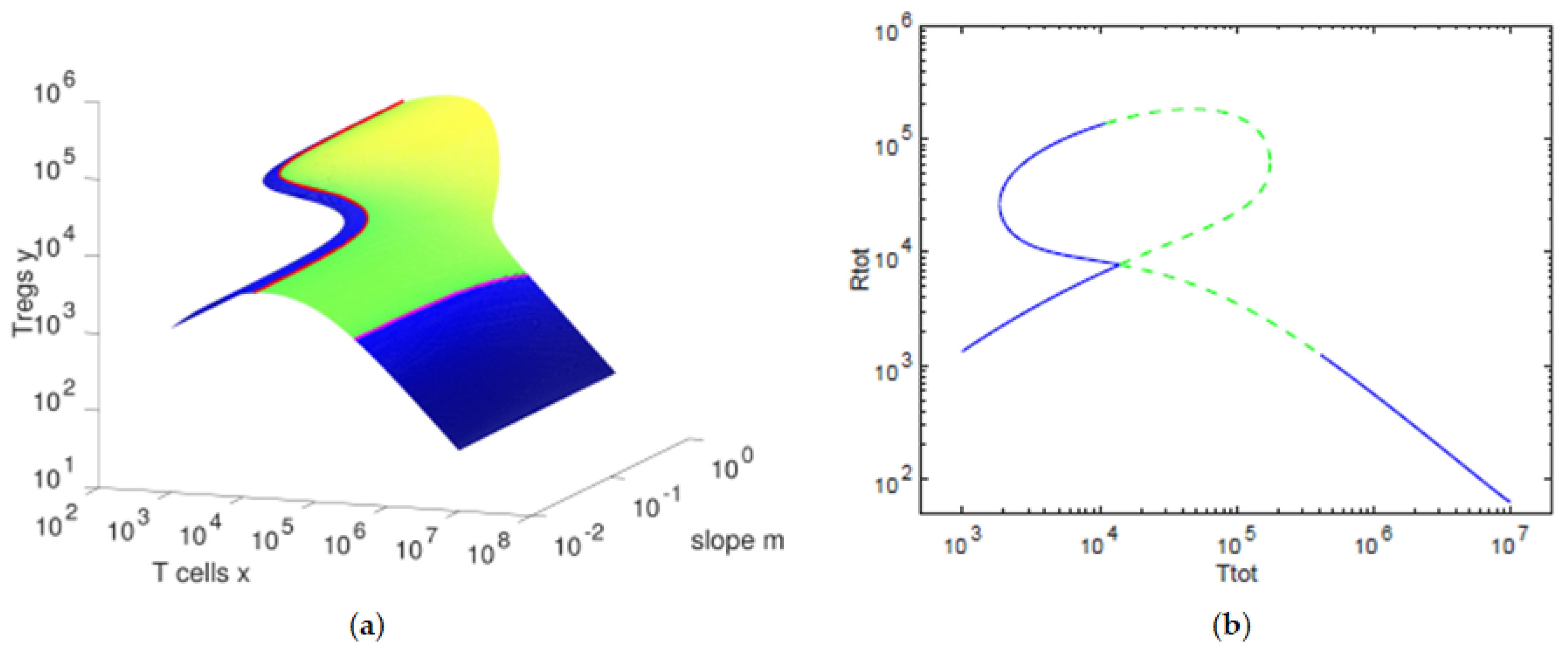
We observe that the balance between the concentration of T cells and that of Tregs varies with the slope parameter m. For the default values of the parameters, we observe that, for lower values of the slope m, a hysteresis is present with its bistability region.

As we further increase the slope, we find up to three possible values of the concentration of the Tregs for each value of the concentration of T cells. In Figure 1, Figure 2 and Figure 3, we can observe the equilibria manifold and its cross-sections for $m=0.2765$.

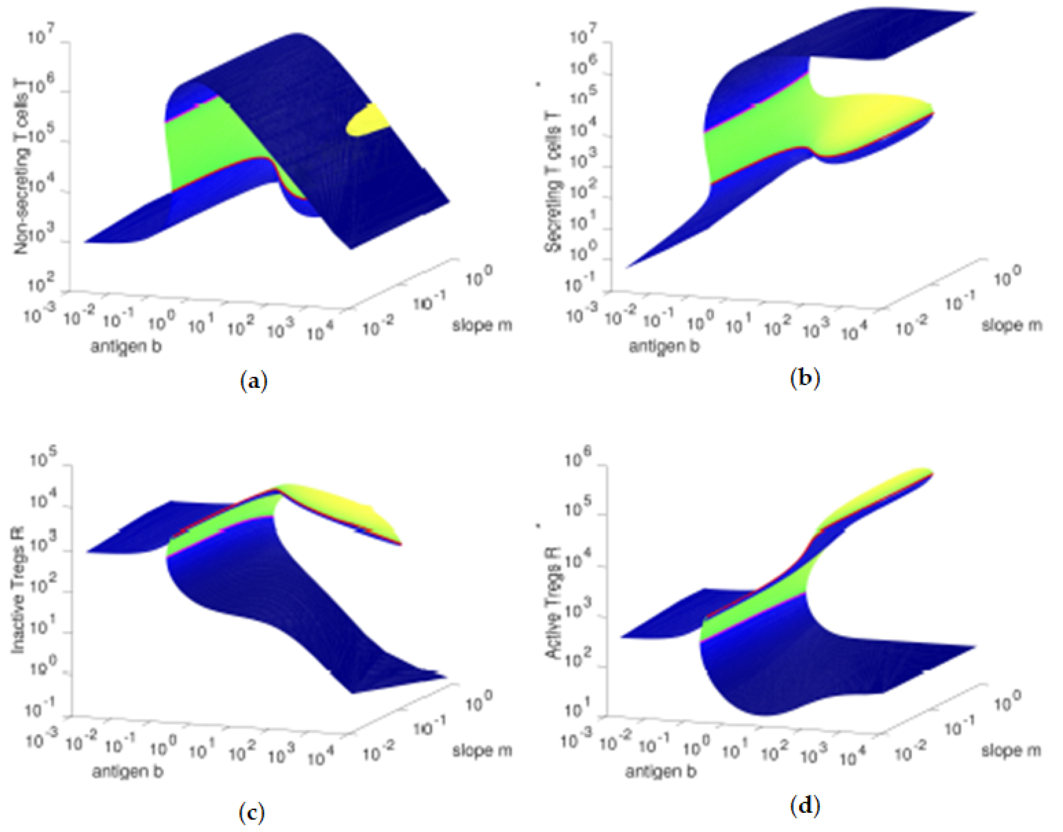
We observe in Figure 1 that the concentration of Tregs y is lower when the concentration of T cells x decreases towards ${10}^3$ and when the concentration of T cells x increases toward ${10}^7$. In Figure 2, we can verify that, for high values of the antigenic stimulation b of T cells, the concentration of T cells x is high and the concentration of Tregs y is low, corresponding to an immune response state of the T cells. The controlled state of the T cells is present for low values of the antigenic stimulation b of T cells, being characterized by low values of the concentration of T cells x and concentrations of Tregs y close to their homeostatic values $R_{hom}$. For intermediate values of the antigenic stimulation b of T cells, we can observe a bistability region, with one equilibria presenting high concentrations of Tregs y and intermediate concentrations of T cells x and the other equilibria being an immune response state. In Figure 3, we observe that, for higher values of the antigenic stimulation b of T cells, the concentration of inactive Tregs R is higher (and the concentration of active Tregs $R^{*}$ is lower) for lower values of the slope parameter, due to the lower antigenic stimulation $\widehat{a}$ of Tregs. As we increase the antigenic stimulation b of T cells from lower values to higher values, initially we observe an increase in the concentrations of the four cell types, which is supported by the increasing concentrations of secreting T cells $T^{*}$ and the correspondent increase of IL-2 cytokines (data not shown).

However, higher values of the antigenic stimulation b of T cells will lead to even larger numbers of cells, which will make more relevant the Fas-FasL induced (quadratic) death. The resulting immune response state is dominated by the compartment with the fittest cells: the secreting T cells $T^{*}$, since these have the highest growth rate and the lowest death rate among the four cell types studied here.

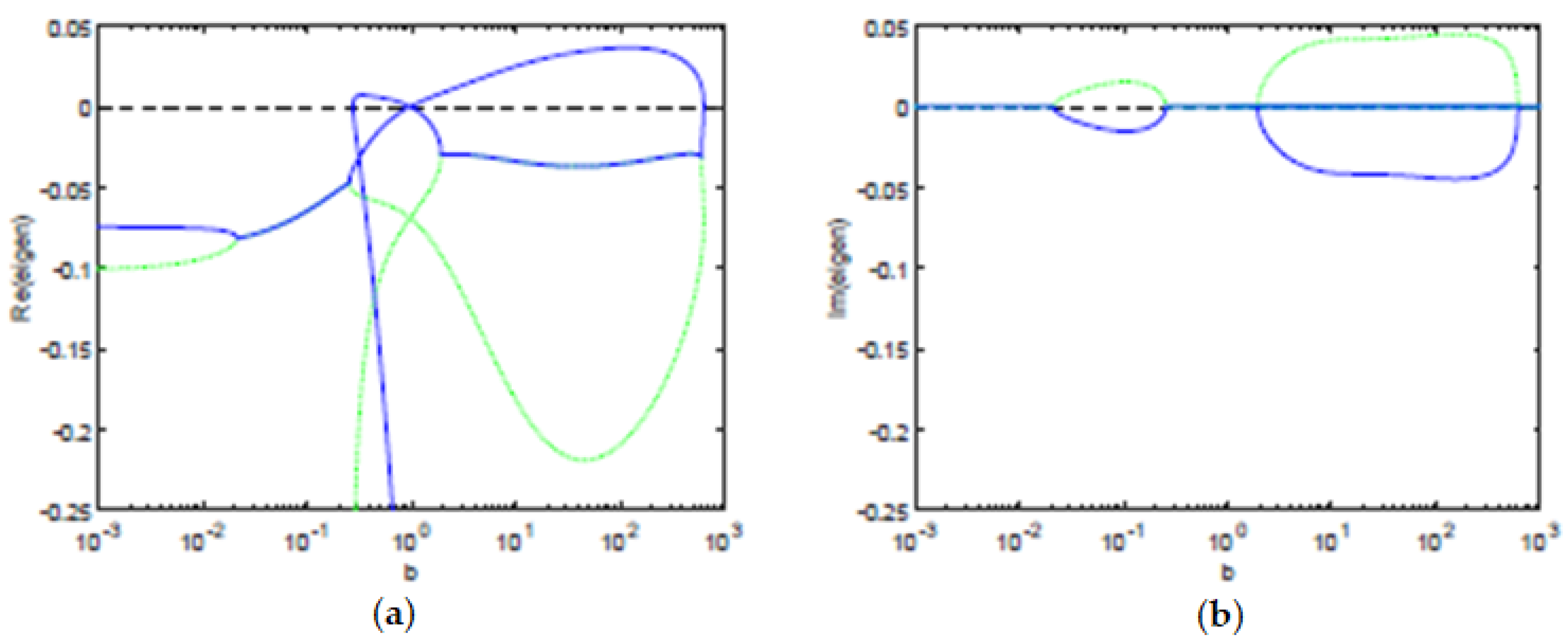
We computed numerically the eigenvalues (see Figure 4) using the Jacobian of the ODE system, in terms of the pair $(x,y)$. We observe that, for the parameters considered, using the balance equation, we have that the concentration of Tregs y is also a multi-valued function of the concentration of T cells x (see Figure 2). Hence, the stability of the equilibria and the bifurcation boundary can be characterized only in terms of the concentration of T cells x. By Theorem 1, all the equilibria points are characterized in terms of the pairs $(x,y)$ satisfying the balance equation. Thus, their stability (or instability) is also dependent on $(x,y)$. The bifurcation boundary $\mathcal{B}$ is the set of equilibria points $(R,R^{*},T,T^{*},I)$ with the property that at least one of the eigenvalues has real part equal to zero and all the other eigenvalues have a non-positive real part. Therefore, using Theorem 1, the bifurcation boundary $\mathcal{B}$ can be fully characterized in terms of the pairs $(x,y)$ satisfying the balance equation. By Theorem 1, the antigenic stimulation of T cells (parameter b) is fully characterized by the pair $(x,y)$ satisfying the balance equation. Hence, the projection of the bifurcation boundary $\mathcal{B}$ in the antigenic stimulation of T cells, is well characterized, resulting in a lower threshold $b_L$ and a higher threshold $b_H$ of antigenic stimulation of T cells (see Figure 4).

The eigenvalues allow us to determine the stability of the equilibria and the time dynamics in a neighborhood of the equilibria. For an antigenic stimulation of T cells below the threshold $b_L$, we observe one stable equilibrium, a controlled state, with a low concentration of T cells. For an antigenic stimulation of T cells above the threshold $b_H$, there is a stable equilibrium, an immune response state, with a high concentration of T cells. Between the two antigenic thresholds, $b_L$ and $b_H$, we find intervals with two stable equilibria, an immune response state, and a controlled state. In the same interval, we also observe one unstable equilibrium, for intermediate concentrations of T cells, that belongs to the separatrix of the basins of attraction of the stable equilibria. When the slope parameter is $m=m_{TC}\approx 0.2765$, the relationship between the variables and the antigenic stimulation b of T cells has two saddle-node bifurcations that bound the bistability region, for $(x_L;y_L;b_L)\approx (4.1\times {10}^5;1.2\times {10}^3;2.8\times {10}^{-1})$ and $(x_H;y_H;b_H)\approx (1.1\times {10}^4;1.4\times {10}^5;6.4\times {10}^2)$. Moreover, there is a transcritical bifurcation at $(x_{TC};y_{TC};b_{TC})\approx (1.4\times {10}^4;7.8\times {10}^3;9.8\times {10}^{-1})$; see Figure 1, Figure 2, Figure 3 and Figure 4. For values of m in a neighbourhood of $m_{TC}$, when we set m at a value below $m_{TC}$, as we increase the antigenic stimulation b of T cells, there will appear a gap along the direction of the antigenic stimulation b of T cells. Thus, we can observe a hysteresis and an isola—present for antigenic stimulations of T cells $b>b_{TC}$. Further decreasing m will lead to a decrease in the size of the isola, until we observe that the the isola vanishes in an isola-center bifurcation at $m=m_I<m_{TC}$. Setting $m>m_{TC}$, as we increase the antigenic stimulation b of T cells, we observe that the hysteresis does not touch itself and has a gap in the direction of the concentration of T cells x. See Burroughs et al. [20] for further details.

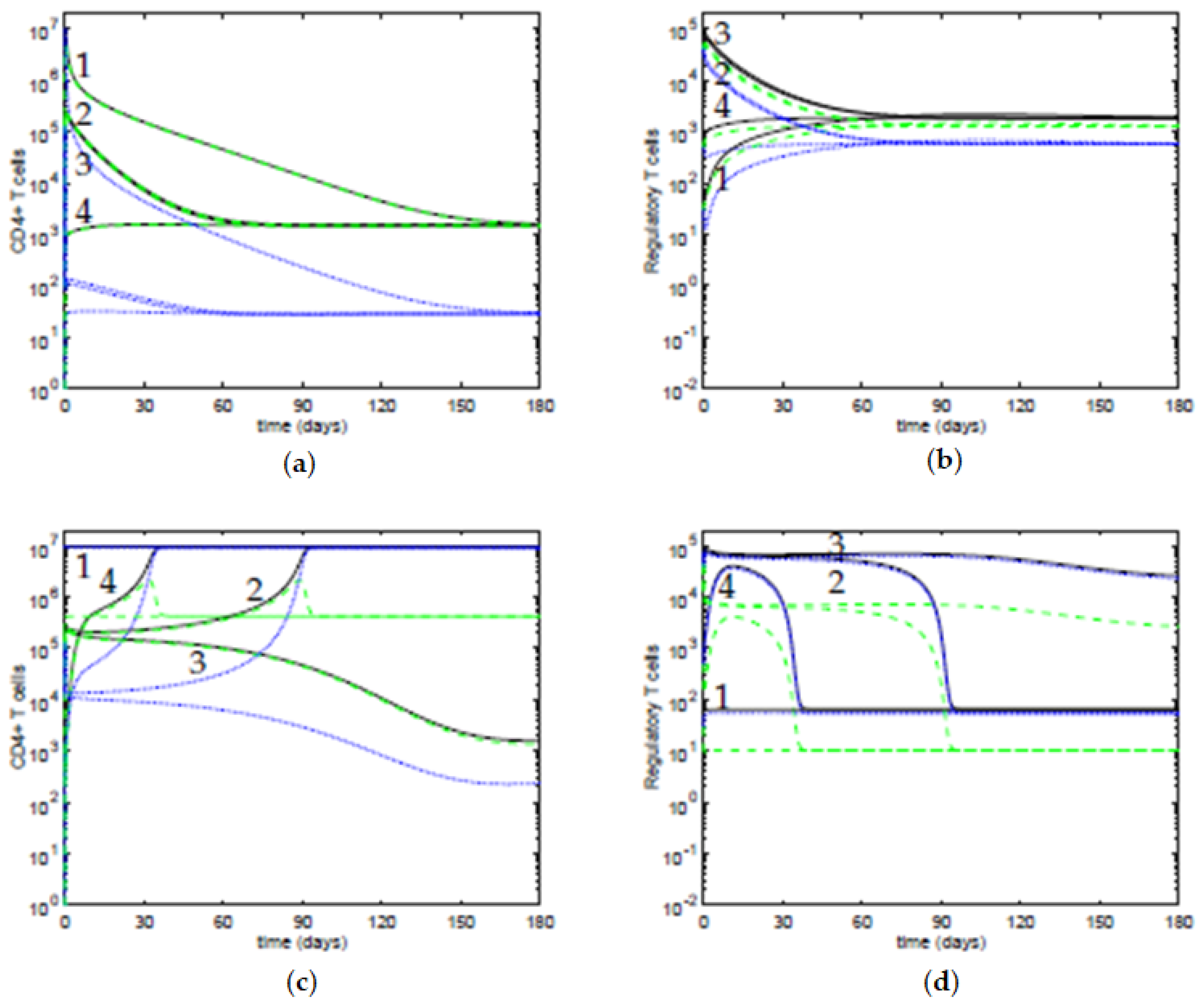
5. Time Evolutions

We present some time evolutions of the ODE system, see Figure 5, considering the four initial conditions in

Table 2. Initial conditions for the time evolutions. Note that the initial condition 2 has higher T cell concentrations and lower Tregs concentrations than the initial condition 3.

Initial Condition	$\mathit{R}$	${\mathit{R}}^{\mathbf{*}}$	$\mathit{T}$	${\mathit{T}}^{\mathbf{*}}$	$\mathit{I}$
1: immune response	30	30	0	${10}^7$	200
2: intermediate +	$4.0\times {10}^4$	$4.0\times {10}^4$	$1.3\times {10}^5$	$1.3\times {10}^5$	6
3: intermediate -	$4.5\times {10}^4$	$4.5\times {10}^4$	$1.2\times {10}^5$	$1.2\times {10}^5$	5
4: controlled	500	500	${10}^3$	0	0

.

In Figure 5a,b, the value of the antigenic stimulation of T cells is low, $b={10}^{-1}$, and the slope parameter is $m=0.2765$; the other parameters are at the default values in Table 1. For these values of the parameters, there is only one stable steady state, a controlled state of the T cells, and the four initial conditions approach it. In Figure 5c,d, the value of the antigenic stimulation of T cells is $b=30$ and the slope parameter is $m=0.2765$; the other parameters are at their default values. For these values of the parameters, there are two stable steady states: an immune response state of the T cells and a controlled state of the T cells. We observe that the initial conditions 1, 2, and 4 approach an immune response steady state; and the initial condition 3 approaches a controlled steady state, with low concentrations of T cells. Moreover, although the initial conditions 2 and 3 are close, their time evolutions diverge from each other, indicating that they belong to distinct basins of attraction of the equilibria. For the initial condition 4, although it starts with a low concentration of T cells, the inhibition by the active Tregs is insufficient to maintain the T cells controlled, thus the system approaches the immune response steady state, after a transient period. Regarding the time dynamics, when the values of the antigenic stimulation of T cells b are such that the eigenvalues have a negative real part and a nonzero imaginary part, the trajectories in the neighborhood of the equilibria approach it in a spiraling trajectory in the direction of the plane determined by the corresponding eigenvectors, and the time dynamics can have damped oscillations. In particular, this behavior can be observed near the controlled equilibria, for values of the concentration of T cells $x<2\times {10}^4$, and for values of antigenic stimulation of T cells b between ∼$2.1\times {10}^{-2}$ and ∼$2.5\times {10}^{-2}$, and for b between ∼$1.9$ and ∼$6.1\times {10}^2$, though with periods of oscillations larger than 100 days, and with a marked decay of the amplitude in each period (data not shown).

6. Conclusions

We studied an immune response model with CD4${}^{+}$ T cells and CD4${}^{+}$ Tregs. We assumed asymmetric death rates and considered that the antigenic stimulation of Tregs $\widehat{a}$ is a linear function of b. We have deepened previous findings, in particular those in the numeric study by Burroughs et al. [20] and the approximate expressions by Oliveira et al. [23]. Here, we presented explicit formulas that describe the exact relationship at equilibria (stable or unstable) between the concentration of T cells, Tregs, IL-2 cytokine, and the antigenic stimulation of T cells. Furthermore, we also showed the Jacobian matrix that allowed the computation of the eigenvalues and the stability of the equilibria. When we changed the antigenic stimulation of T cells parameter, we observed a hysteresis with a bistability region and a transcritical bifurcation, for a given value of the slope of the tuning parameter. Moreover, we present some time evolutions for some values of the parameters. This type of model, with two clonotypes of T cells, was applied to study the appearance of autoimmune responses due to bystander proliferation of T cells, as in Burroughs et al. [21] and the suppression of of autoimmunity, as in Oliveira et al. [24]. Additionally, the hysteresis, present for the parameter values we used, indicates that treatment of autoimmunity might require a high level of immune suppression. However, immune suppressive drugs that deplete significantly the concentration of CD4${}^{+}$ T cells might concomitantly decrease the concentration of Tregs. If this happens to be the case, this treatment might not bring the system into the basin of attraction of the controlled steady state. Hence, it is possible that, after the immune suppressive treatment, the system might be in a state similar to the initial condition 4, where apparently the T cells are controlled, but, as we observe in Figure 5c,d, after a transient time, the concentrations of T cells approach instead the immune response steady state. Furthermore, for parameters in a neighborhood of the transcritical bifurcation point, and considering an initial condition near the controlled steady state, it is possible that a small perturbation might bring the system across the separatrix of the basins of attraction. Thus, CD4${}^{+}$ T cells will be able to escape control and, after some transient period, the system will approach the immune response steady state. Nevertheless, in silico models can be useful in simulating innovative therapies, which makes room for only the more promising ones being considered to be studied in in vivo experiments.