Dominance-Based Decision Rules for Pension Fund Selection under Different Distributional Assumptions

Abstract

The pension landscape is changing due to the market situation, and technological change has enabled financial innovations. Pension savers usually seek financial advice to make a personalised decision in selecting the right pension fund for them. As such, decision rules based on the assumed risk profile of the decision maker could be generated by making use of stochastic dominance (SD). In the paper, the second-pillar pension funds operating in Lithuania and Slovakia are analysed according to SD rules. The importance of the distributional assumption is explored while comparing the results of empirical, student-t, Hyperbolic and Normal Inverse Gaussian distributions to generate SD-based rules that could be integrated into an advisory solution. Moreover, due to the differences in SD results under different distributional assumptions, a new SD ratio is proposed that condenses the dominance-based relations for all considered dominance orders and probability distributions. The empirical results indicate that this new SD ratio efficiently characterises not only the preference of each fund individually but also of a group of funds with the same attributes, thus enabling multi-risk and multi-country comparisons.

1. Introduction

Most EU countries have carried out systemic pension reforms over the last decades to maintain fiscal sustainability in the face of aging populations, declining fertility rates and global migration trends. In response to these pressures, these countries have enacted mandatory or quasi-mandatory pension plans, both public and private, based on the so-called defined contribution scheme, thus diversifying retirement income sources across providers. One can find numerous typologies for retirement-income systems, but the most commonly used approaches are the World Bank (WB) and Organisation for Economic Cooperation and Development (OECD) frameworks [1]. A three-pillar pension system concept was established by the WB in 1994, with a large role given to private individual pension accumulation [2]. The five-pillar concept was developed in 2005 and has since been adopted by many countries in Europe [3]. Alternatively, the OECD has designed a taxonomy that has two mandatory tiers, i.e., redistributive and insurance tiers. This approach aims for a global classification for pension schemes that is consistent over a range of countries with different retirement-income systems. As there is no one-size-fits-all approach, country-specific conditions require the adoption of selected frameworks defined in such a manner as to best suit particular countries. In the current paper, we follow the WB’s three-pillar approach, as it is more commonly used in the countries that are considered in the following analysis. It is worth mentioning that, in most countries, a national regulator plays an important role in determining the criteria and rules that pension fund management companies must follow.

Shifting from a conventional pension scheme to private pension plans requires individuals to make investment decisions mainly by themselves, which is a challenging task. There are several reasons the choice of a pension fund is complicated. First, due to a lack of financial literacy and understanding, a participant might select an inappropriate fund for their pension savings [4,5]. In response to this problem, pension fund managers usually report simple descriptive statistics, accompanied by some explanations, related to the historical performances of their pension funds, but no deeper analyses or forecasts are published. However, these reports are typically limited to the pension funds managed by a certain company. Notably, the managers use some benchmarks against which the performances of their pension funds are compared rather often. Unfortunately, benchmarks’ compositions are not strictly regulated; therefore, global comparisons of pension fund performances are difficult to make. Consequently, the difficulties in making comparisons between funds constitute a second reason fund selection is challenging. Finally and crucially, pension funds managed by different companies usually exhibit different performance results, even though all of them operate under the same market conditions [6,7], which means that the actual investment performance might be different according to the specified investment strategy. As such, it might be assumed that the targets achieved by private pension funds depend on how well they are managed. Obviously, while multi-pillar pension systems have been established to diversify risks, such as demographic change, labour market dynamics and public finances, the investments in private pension funds are now exposed to changing financial returns, market volatility and inflation.

While many authors focus on Asset-Liability Management (ALM) for pension funds [8,9,10,11,12,13,14,15,16], this paper makes a contribution in the modelling field by attempting to identify the best investment choice for a participant who wishes to maximise the expected utility of their retirement benefits on the basis of their risk profile. One way to address this issue is to provide some exploratory analysis with a special focus on risk measurement and performance evaluation [17], thus allowing the participant to choose the pension fund complying with their risk considerations. Following this path, many case studies have been published that typically include the analysis of pension funds operating in a certain country, e.g., Lithuania [7], the Czech Republic [18], Croatia [19] and so forth. Consequently, some technique can be employed to assess or classify the pension funds considered in the analysis. For example, one can use multi-criteria optimisation techniques [20], data envelopment analysis [21] or some stochastic dominance approach [22].

In view of this approach, the current paper considers the second-pillar pension funds (PFs) with the aim of determining which fund is the most preferable for a participant on the basis of his risk profile. To make the decision, one can rely on descriptive statistics, risk measures and performance ratios of the PFs’ returns [23,24,25,26]. Unfortunately, all these estimates limit the information about the probability distribution of returns to a single number. Therefore, we propose a methodology based on stochastic dominance (SD), allowing us to compare funds while employing the whole distribution of the returns, regardless of whether it is estimated in a parametric or non-parametric manner. As recently shown by Moriggia et al. [8] and Kopa et al. [27], stochastic dominance is a useful tool in pension fund selection and provides interesting results. In this paper, we consider three different types of SD relations, specifically first-order SD (FSD), second-order SD (SSD) and third-order SD (TSD) [22,28,29], to describe different risk profiles for a participant. The analysis covers the period 2011–2018. In particular, the pension funds operating in two countries, Lithuania and Slovakia, are compared under different distributional assumptions. We chose these two countries because: (i) they are close to each other in terms of geographical, historical, macro-economical and sociological indicators; (ii) their second-pillar PFs have not yet been analysed using utility (stochastic dominance) tools; and (iii) their pension systems have not been compared previously. In particular, empirical, student-t, hyperbolic and normal-inverse Gaussian (NIG) distributions are used to describe the PFs’ returns. In fact, in the last few decades, many papers have published evidence of the non-normality (see [30,31,32]) and fatness (see [5,33,34]) of financial time series. Furthermore, some researchers have found evidence that the tails of returns are typically semi-heavy (see [35,36,37]) from a class of generalised hyperbolic distributions, which includes the student-t, hyperbolic and NIG distributions. Additionally, Huang [38] explained the differences between the above distributions based on the tail behaviour. The exponential decay of hyperbolic distribution tails is slower than that for the tails of the NIG distribution, which are semi-heavy and non-identical (depending on the asymmetry parameter). Comparatively, a three-parameter Student-t distribution is well known and useful in theoretical analysis due to its nice probability density function, balancing as it does between super-heavy (when the degrees of freedom $\nu \to 0$) and Gaussian behaviour (when $\nu \to \infty$).

The rest of the paper is organised as follows. Section 1.1 provides an overview of the multi-pillar pension systems currently operating in Lithuania and Slovakia. Section 2 presents the research methodology used in the analysis. The theoretical background for stochastic dominance is described in Section 2.1. This background is followed by a brief overview of the semi-heavy tailed probability distributions used in the analysis as a tool to model the returns’ distribution. A newly derived stochastic dominance ratio based on pairwise stochastic dominance is presented in Section 2.6, and the experimental design is outlined in Section 2.7. Section 3 presents the performance analysis of the pension funds using risk measures, the results of pairwise stochastic dominance based on empirical and theoretical probability distributions and, most importantly, the search for the most preferable pension fund based on the derived SD ratio. Finally, a discussion of the results and future steps are provided at the end of the paper.

1.1. Pension Systems in Lithuania and Slovakia

Lithuania and Slovakia have both undertaken systematic pension reform by adopting the WB’s three-pillars approach, which is designed to achieve desired societal and individual benefits while minimising the relevant risks. In general, these pension schemes provide three distinct sources of accumulation for retirement funds.

Lithuania began its pension reform in 2004 by introducing Pillars II and III to the pension system. However, the PAYG pillar (state pension, Pillar I) still plays a dominant role in ensuring income for old-age pensioners. At the end of 2012, this system was reformed due to the financial crisis. Recently, by July 2019, pension funds managed by pension accumulation companies must have been reorganised to implementing the life-cycle approach. No occupational pensions are available in Lithuania [39,40].

In Slovakia, the pension reform started in 1996 with the introduction of Pillar III, which, at that time, was organised as a voluntary pension pillar. Later, Pillar III was reorganised to accommodate a more personal approach with the financial support of employers. The WB’s approach was fully implemented with the introduction of Pillar II, a defined contribution pension saving scheme, at the beginning of 2005. In terms of terminology, it is called the “1bis pillar”, as individual retirement accounts are funded via a partial redirection of social security contributions to individual pension savings accounts [39,41].

The basic data on the pension system set-ups in these two countries are summarised in

Table 1. Comparison of Lithuanian and Slovak pension systems (cut-off year 2018).

	Pillar I	Pillar II	Pillar III
	Lithuanian pension system
Scheme	PAYG defined benefit scheme	Funded scheme	More flexible funded scheme
Manager	State Social Insurance Fund (SoDra)	Pension accumulation companies	Pension accumulation companies
Participation	Mandatory	Quasi/Mandatory	Voluntary
Coverage	Almost 100%	92.78%	4.38%
Funds offered		20	12
Contribution rate	25.30%	min 2% and max 6%
Quick facts:	Average pension: EUR 344.20; Replacement ratio: 39.41%; Retirement age—63.6 years for men and 62.3 years for women
	Slovak pension system
Scheme	PAYG State pension	Occupational pensions—defined contribution	Individual pensions—fully funded defined contributions
Manager	Social Insurance Company	Pension Asset Management Companies	Pension Asset Management Companies
Participation	Mandatory	Voluntarily up the age of 35/Mandatory	Voluntary
Coverage	Almost 100%	60.00%	27.00%
Funds offered		19	15
Contribution rate	13.50%	4.50%
Quick facts:	Average pension: EUR 455; Replacement ratio: 46%; Retirement age—62.4 years

, which is in line with the research report [39].

As shown in Table 1, the overall coverage provided by Pillar II, measured as a ratio between the number of participants and the economically active population (number of insured persons in Pillar I), is almost 93% in Lithuania and 60% in Slovakia, indicating the importance of these funds, particularly since future pension incomes might be mostly influenced by Pillar II savings. Comparatively, Pillar III is expected to generate retirement income for less than 30% individuals in Slovakia, and, obviously, an insignificant portion for Lithuanian savers. This fact is the main reason we decided to begin with an analysis of Pillar II. In the future, a portfolio management task could be considered for inclusion in order to diversify retirement income sources and achieve maximum worth.

Regarding the challenging task of selecting a suitable pension fund for an individual, one possible option is to carry out pension fund selection according to a predefined investment strategy (see

Table 2. Funds arranged into four groups based on the investment strategy.

Lithuanian Funds [40]	Slovak Funds [the Act on Old-Age Saving No. 43/2004]
Conservative investment funds;	Bond guaranteed mandatory pension funds;
Funds investing up to 30% of assets in equity;	Mixed mandatory pension funds (since March 2005);
Funds investing up to 70% of assets in equity;	Equity mandatory pension funds (since March 2005);
Funds investing up to 100% of assets in equity.	Index mandatory pension funds (since April 2012).

) that theoretically reflects its riskiness.

Such classifications (see Table 2) typically help determine the risk category a pension fund should be placed in, but, obviously, the performance of any pension fund is highly dependent on how its investment strategy has been implemented historically. It has already been demonstrated [7] that the grouping of funds based on the ex-post returns can be different from the scheme provided in the table. Furthermore, even if the decision on the type of pension fund has already been made, the next step is to choose one fund within a group, which in comparison is a more complicated task. Therefore, we proceed with the analysis of pension funds over a certain time period using the stochastic dominance approach with the aim to propose the approach for determining the best fund among those being considered. Additionally, we pay a special attention to the comparison of pension funds operating in two countries with a similar pension systems, as well as the different risk groups that emerge based on the investment portfolio.

2. Materials and Methods

This section presents the theoretical background for stochastic dominance (SD) with a special focus on the three SD principles while considering investors’ risk profiles. Since the pension fund returns are treated as random variables, we also recall some theoretical heavy-tailed probability distributions. Then, a new performance ratio based on pairwise stochastic dominance is proposed, one which allows us to identify efficient and inefficient pension funds by discriminating between them on the basis of country and/or risk group.

2.1. Stochastic Dominance Relations

In the current paper, the investor is a participant in the pension system who intends to select a private pension fund as an investment. Stochastic dominance rules as well as other investment rules employ partial information on the investor’s preferences; therefore, they produce only a partial ordering of all the available investments under consideration. Depending on the assumptions on the investor’s preferences defined by a utility function $u\left(x\right)$, three different types of SD relations are considered:

• First-order stochastic dominance (FSD)—no restriction on the participants utility, and only non-satiation is assumed ($u^{\prime }\left(x\right)\ge 0$);
• Second-order stochastic dominance (SSD)—assumptions of non-satiation and risk aversion are considered ($u^{\prime }\left(x\right)\ge 0$ and $u^{″}\left(x\right)\le 0$ ); and
• Third-order stochastic dominance (TSD)—an additional assumption on the positive skewness preference is imposed ($u^{\prime }\left(x\right)\ge 0$, $u^{″}\left(x\right)\le 0$ and $u^{\prime \prime \prime }\left(x\right)\ge 0$).

We assume that the returns of pension funds are treated as random variables $X_i,i=1,\dots ,N.$. By definition, the random return of the ith fund $X_i$ dominates the random return of the jth fund $X_j$ with respect to XSD ($X_i{\succ }_{XSD}{X}_j$) if E$u\left(X_i\right)\ge$ E$u\left(X_j\right)$ for all $u\in$ XSD where XSD = FSD, SSD, TSD. In particular, if the random return of one fund dominates the random return of another fund, then all investors obeying particular assumptions on their utility functions prefer the dominating fund to the one being dominated or are indifferent between them. Thus, following Levy [22], we can formulate the necessary and sufficient conditions for FSD, SSD and TSD using k-times cumulative distribution functions.

Theorem 1.

Let $F_i\left(x\right)$ be the cumulative distribution function of fund i and let E$X_i<\infty$ for all $i=1,\dots ,N.$ Then,

(i) 

$X_i{\succ }_{FSD}{X}_j$ if and only if $F_i\left(x\right)\le F_j\left(x\right)$, $\forall x;$

(ii) 

$X_i{\succ }_{SSD}{X}_j$ if and only if $F_i^{\left(2\right)}\left(x\right)\le F_j^{\left(2\right)}\left(x\right)$, $\forall x;$

(iii) 

$X_i{\succ }_{TSD}{X}_j$ if and only if $F_i^{\left(3\right)}\left(x\right)\le F_j^{\left(3\right)}\left(x\right)$, $\forall x$; and E$X_i\ge$ E$X_j$

where $F_i^{\left(k\right)}\left(x\right)$ is k-times cumulative distribution function:

$$F_i^{\left(1\right)}\left(x\right)=F_i\left(x\right),F_i^{\left(k\right)}\left(x\right)=\underset{-\infty }{\overset{x}{\int }}{F}_i^{(k-1)}\left(t\right)dt,k=2,3.$$

Since we consider N funds, $P_2^N=\frac{N!}{(N-2)!}$ pairs of funds could be considered for a stochastic dominance comparisons. The number of pairs can be reduced by employing a necessary condition, specifying that the superior investment must have a greater (or equal) mean [28]. As a result, the number of necessary comparisons is reduced to $C_2^N=\frac{N(N-1)}{2}$ combinations.

To begin with, the empirical distribution of the observed returns is considered. Let $X_i^t$ be the return of fund i at time t, $i=1,\dots ,N$, $t=1,\dots ,T$. Assume that all observations are equally probable and that for each fund i we first order the observation such that $X_i^1\le X_i^2\le X_i^T$. Then, the necessary and sufficient condition for FSD and SSD can be simplified as follows.

Theorem 2.

Let $X_i^1\le X_i^2\le X_i^T$ be equiprobable realisations of random return $X_i$, $i=1,\dots ,N.$ Then,

(i) 

$X_i{\succ }_{FSD}{X}_j$ if and only if $X_i^t\ge X_j^t$, $t=1,\dots ,T;$ and

(ii) 

$X_i{\succ }_{SSD}{X}_j$ if and only if ${\displaystyle \sum _{s=1}^t}{X}_i^s\ge {\displaystyle \sum _{s=1}^t}{X}_j^s$, $t=1,\dots ,T.$

To check the TSD relation using the empirical distribution of returns, either the algorithm in [22], which is based on a comparison of three times cumulative distribution functions, or the alternative sufficient condition published in [29] can be utilised.

Next, we proceed with the student-t, hyperbolic and normal-inverse Gaussian distributions, which are briefly introduced in the following sections. Furthermore, we use adaptive numerical integration (using R packages) to check for the pairwise stochastic dominance described in Theorem 1.

2.2. Generalised Three-Parameter Student-t Distribution

Suppose that pension fund’s returns follow the student-t distribution. Then, the probability density function (PDF) is given by

$$p(x,\mu ,\sigma ,\nu )=\frac{\mathsf{\Gamma }\left(\frac{\nu +1}{2}\right)}{\mathsf{\Gamma }\left(\frac{\nu }{2}\right)\sqrt{\pi \nu }\sigma }{\left(1+\frac{1}{\nu }{\left(\frac{x-\mu }{\sigma }\right)}^2\right)}^{-\frac{\nu +1}{2}},$$

where $\mu$ is a location parameter, $\sigma$ is a scale parameter and $\nu$ represents the degrees of freedom.

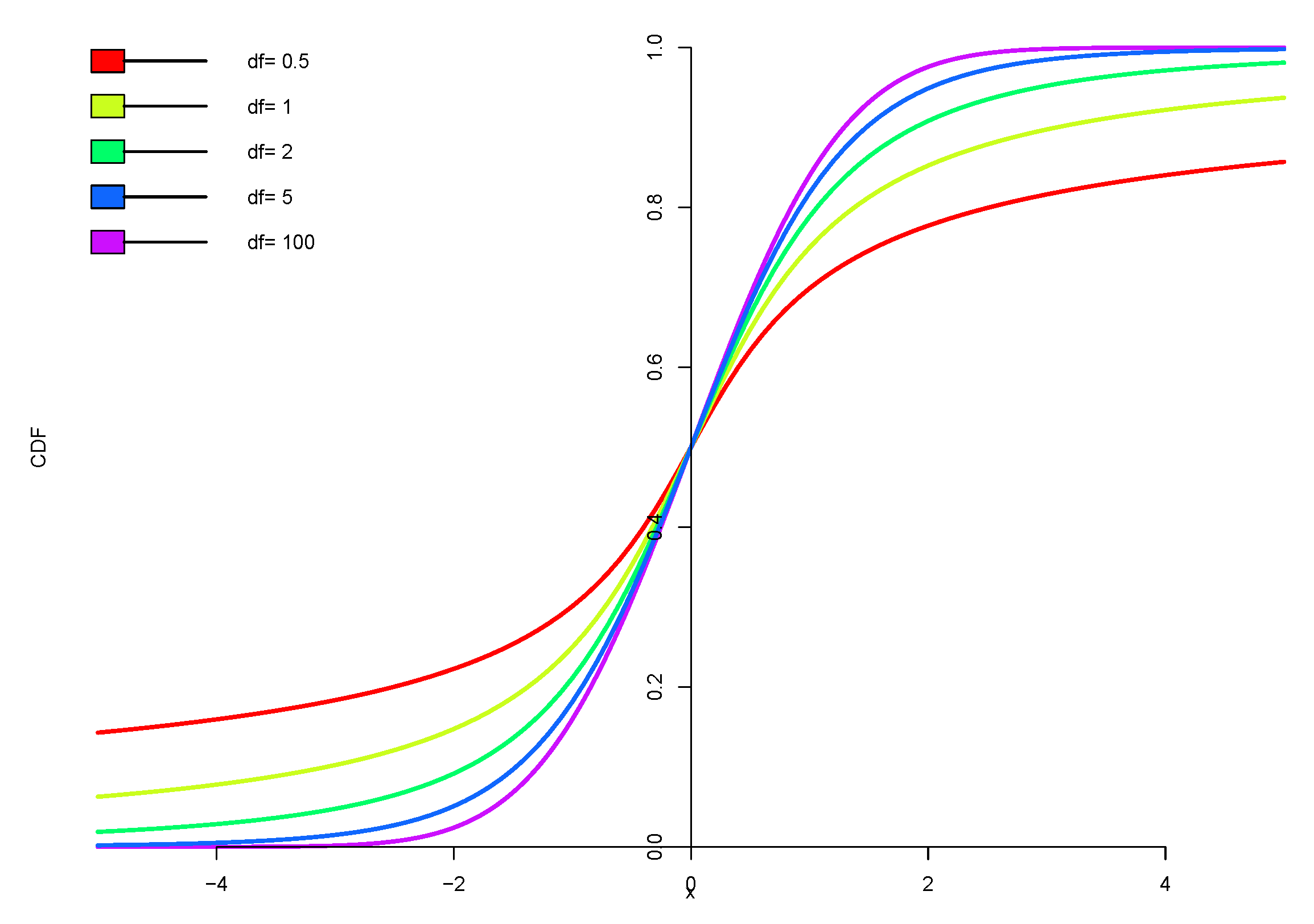
The cumulative distribution function (CDF) of the student-t distribution (see Figure 1) is

$$F(x,\mu ,\sigma ,\nu )=\frac{1}{2}+\frac{(x-\mu )\mathsf{\Gamma }\left(\frac{\nu +1}{2}\right)}{\mathsf{\Gamma }\left(\frac{\nu }{2}\right)\sqrt{\pi \nu }\sigma }{}_2{F}_1\left(\frac{1}{2},\frac{\nu +1}{2},\frac{3}{2},-\frac{{(x-\mu )}^2}{\nu {\sigma }^2}\right),$$

where ${}_2{F}_1$ is a particular case of the hypergeometric function and $\mathsf{\Gamma }(·)$ denotes the Gamma function.

The random variable X has expectation $E\left(X\right)=\mu$ (if $\nu >1$), while the variance $var\left(X\right)={\sigma }^2\frac{\nu }{\nu -2}$ exists only when $\nu >2$.

In general, the tails of the student-t distribution range from the Cauchy distribution ($\nu =1$) to the normal distribution ($\nu =\infty$), depending on $\nu$. Moreover, if $\nu <1$, then the tails become super-heavy; in such case, the expectation does not exist, and the student-t distribution becomes useless in most practical applications.

2.3. Hyperbolic Distribution

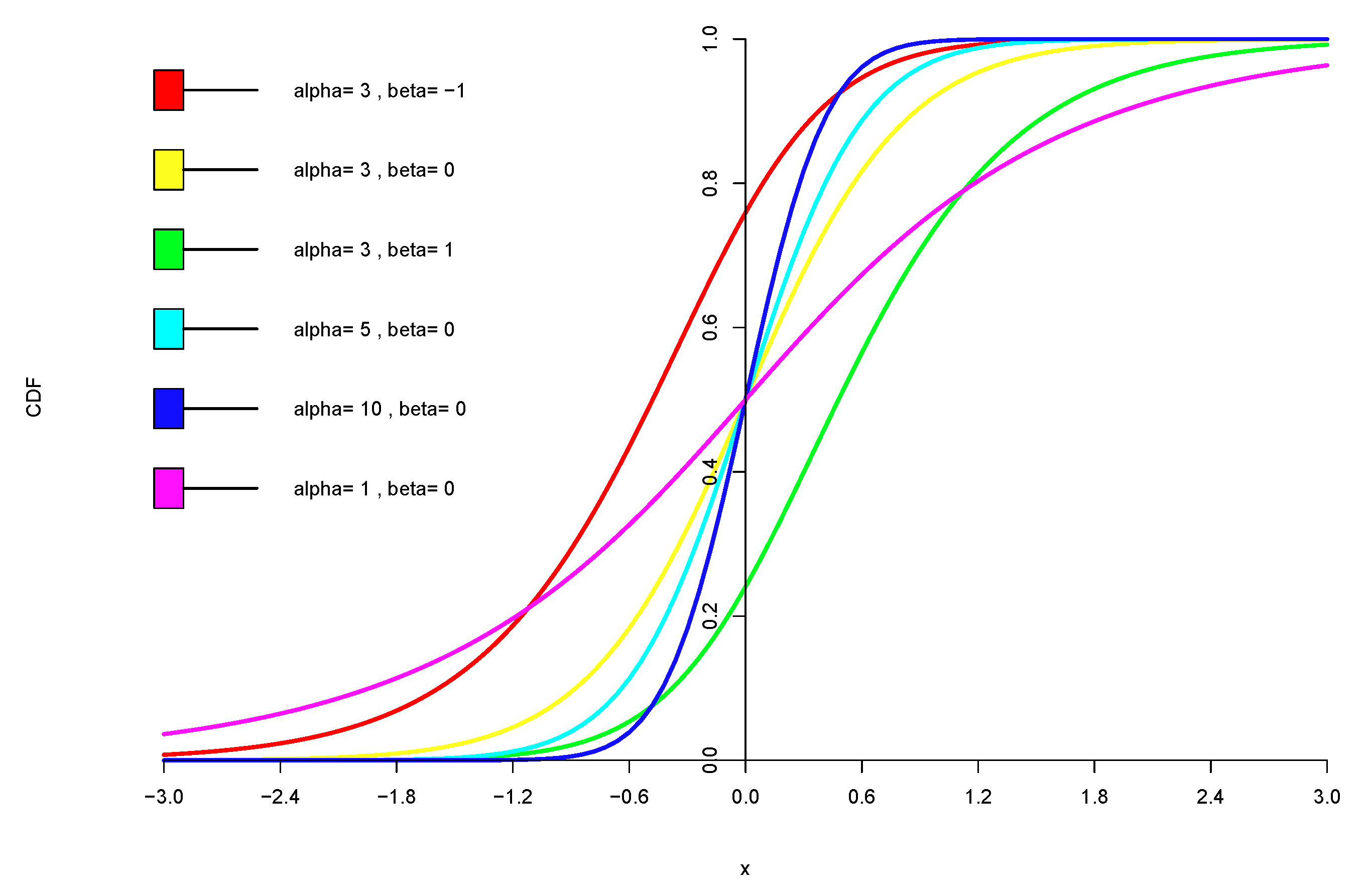
The hyperbolic distribution is a continuous probability distribution (from the generalised hyperbolic distribution family) characterised by the logarithm of the probability density function being proportional to hyperbola. Consequently, the tails of the distribution decrease exponentially, enabling the modelling of returns that are heavier than normal ones. The density of the hyperbolic distribution is given by

$$p(x,\alpha ,\beta ,\delta )=\frac{\sqrt{{\alpha }^2-{\beta }^2}}{2\alpha \delta K_1\left(\delta \sqrt{{\alpha }^2-{\beta }^2}\right)}{e}^{-\alpha \sqrt{{\delta }^2+{(x-\mu )}^2}+\beta (x-\mu )}$$

where $\alpha >0$ is a shape parameter, $0\le \left|\beta \right|<\alpha$ is an asymmetry parameter, $\mu$ is a location parameter, $\delta$ is a scale parameter and $K_1(·)$ denotes a modified first-order Bessel function of the third kind. CDF of Hyperbolic distribution is given in Figure 2.

As a mater of fact, the hyperbolic distribution is a random mixture of normal distributions, i.e., the normal mean–variance mixture with GIG (generalised inverse Gaussian) emerging when $\lambda =1$ [42]. Moreover, when $\alpha \to \infty$, the limiting distribution is also a normal distribution. Finally, when $\alpha \to 0$, the limiting distribution is a skewed and shifted Laplace distribution.

2.4. Normal Inverse Gaussian Distribution

The normal-inverse Gaussian (NIG) distribution is a continuous probability distribution that is defined as a normal variance–mean mixture, where the mixing density is the inverse Gaussian distribution (i.e., GIG when $\lambda =-1/2$). The NIG distribution is more practical than the hyperbolic distribution, due to its convolution properties, and it still has semi-heavy tails. Moreover, the NIG distribution is more useful in linear dependence modelling than the other generalised hyperbolic distributions.

The probability density function for the NIG distribution is given by

$$p(x,\alpha ,\beta ,\mu ,\delta )=\frac{\alpha \delta K_1\left(\alpha \sqrt{{\delta }^2+{(x-\mu )}^2}\right)}{\pi \sqrt{{\delta }^2+{(x-\mu )}^2}}{e}^{\delta \sqrt{{\alpha }^2-{\beta }^2}+\beta (x-\mu )}$$

where $\alpha$ is a tail parameter, $\beta$ is an asymmetry parameter, $\mu$ is a location parameter, $\delta$ denotes a scale parameter and $K_1(·)$ denotes a modified first-order Bessel function of the third kind.

As for all generalised hyperbolic distributions, the NIG distribution converges to a normal distribution when $\alpha \to \infty$. Under a certain condition when $\alpha \to 0$, the limiting distribution is a scaled and shifted Cauchy distribution. CDF of Hyperbolic distribution is given in Figure 3.

The NIG distribution is especially useful in cases in which the tails observed are not “too heavy”, while the hyperbolic distribution captures more heavier tails well.

2.5. Performance Analysis of Pension Funds Using Point Estimates

The financial literature provides abundant choices in terms of the risk measures and performance ratios to be used in the analysis of investment alternatives. As such, some authors suggest that they can be categorised into particular groups, such as reward-to-variability ratios, extreme risk measures, reward-to-risk ratios, partial moments and so on, based on what characteristics from the distribution of returns are used in their formulas. In the current paper, we use some of these measures as the representatives of the particular classes that are most often used in frontier research. Notably, a conventional measure that has been used for a certain period to evaluate the risk is the standard deviation (or dispersion). Since the standard deviation penalises both the upside and the downside potential of an asset’s return symmetrically, it is not recommended as a measure of performance in a non-Gaussian (non-symmetric) setting.

One of the most popular risk measuring concepts is the Value-at-Risk (VaR), which describes the maximum loss over a target horizon within a given confidence level [43]. As such, it can be included in the set of extreme risk measures since it captures the downside risk in a single figure by focusing on the tail of a return distribution. However, the VaR has been criticised heavily for not being a coherent risk measure. Consequently, some new measures have been derived from the VaR. For example, a popular measure is Conditional Value-at-Risk (CVaR), which quantifies the expected losses that occur beyond the VaR cutoff. Comparatively, while the VaR is a frequency-based estimate, the CVaR is the severity-based measure that is still to be minimised by risk-averse investors.

Due to its simplicity and ease of interpretation, the Sharpe Ratio has become one of the most widely used reward-to-variability performance measures. It is the ratio between the mean and the standard deviation of the portfolio’s return [44]. Many alternatives to the Sharpe ratio have been proposed in the literature [24]. One such alternative is the Sortino ratio, in which the negative deviation from the mean return is considered as a measure of variability instead of the standard deviation [26]. Specifically, an investment option with a higher Sharpe or Sortino ratio is considered to be superior to its alternatives.

Unlike the reward-to-variability ratios, a Rachev ratio is a reward-to-risk performance measure that was developed to measure the right-tail reward relative to the left-tail risk in the worst $\alpha \times 100$% cases [25]. Obviously, this is a performance measure that investors wish to maximise.

Many researchers has been devoted to finding the right risk or performance measure, but it is believed that such a perfect measure does not exist because such measures typically depend on at most two parameters to describe the complexity of a distribution [45]. However, most decision makers have some common beliefs and perceptions involving risk.

2.6. Performance Ratio Based on Pairwise Stochastic Dominance

To help a pension system participant choose the most preferable fund among all available funds (random variables), we propose the following ratio R.

Definition 1.

The stochastic dominance ratio $R_i$ of random variable ${\xi }_i$ is defined as

$$R_i=\frac{D_i^{+}-D_i^{-}}{D_i^{+}+D_i^{-}},i=1,..,N;$$

(1)

where N is the total number of random variables, $D_i^{+}$ is the number of stochastic dominance relations in which ${\xi }_i$ dominates another variable for some probability distribution and SD order and $D_i^{-}$ is the number of dominance relations in which ${\xi }_i$ is dominated by another variable for some probability distribution and SD order.

More precisely,

$$D_i^{+}=\sum _{j=1}^N\sum _{k=1}^K\sum _{m=1}^M{C}_{ij}^{km}\mathrm{and}{D}_i^{-}=\sum _{j=1}^N\sum _{k=1}^K\sum _{m=1}^M{C}_{ji}^{km}$$

(2)

where $C_{ij}^{km}$ are matrices of SD pairwise comparisons according to the distribution k and SD rule m, K is the number of distributions assumed and M is the number of SD rules used, i.e., $C_{ij}^{km}=1$ if fund i dominates fund j with respect to the mth order SD using the kth probability distribution and $C_{ij}^{km}=0$ otherwise. In our experiment, we use $N=37$ pension funds; $K=4$ since empirical, student-t, hyperbolic and NIG distributions are analysed; and $M=3$ since three SD rules (FSD, SSD and TSD) are employed. In total, 12 matrices $C_{ij}^{km}$ represent the pairwise comparisons summarised in the Figure of Section 3.7.

The proposed ratio $R_i$ is equal to 1 if the fund i dominates at least one other fund and is not dominated by the other funds $j=1\dots N,(j\ne i)$ available. In this case, the fund i is regarded as the efficient fund since it outperforms at least some other fund and is dominated by no other fund. If there are several funds with $R_i=1$, then the most preferable fund is the one with the greatest $D_i^{+}$ value since it then dominates more funds. Furthermore, the ratio $R_i$ is equal to $-1$ if fund i is dominated by at least one other fund j ($j\ne i$) and does not dominate any other fund. In this case, fund i is regarded as a bad fund (the most inefficient), since it dominates no other fund and at least one fund exists that dominates it. All other values of ratio $R_i$ are in the interval $(-1;1)$.

Moreover, if we aim to compare how funds, on average, perform in a particular country, we can estimate the average R ratio.

Definition 2.

The average stochastic dominance ratio over set h is defined as

$${\overline{R}}^h=\frac{1}{N_h}\sum _{i=1}^{N_h}{R}_i;$$

(3)

where h denotes the set indicator and $N_h$ is the number of elements in set h.

In this paper, h denotes the country we are interested in and $N_h$ is the number of funds operating in country h.

Furthermore, the country indicator h can be easily substituted by a risk profile indicator or even a fund manager indicator. Such averaging is useful in the detailed comparison of funds and should facilitate the selection of a pension fund or fund manager.

2.7. Experimental Design

In this section, we describe the detailed scheme used in our experiment.

According to the literature review, empirical analyses and parameterisation results of pension fund returns, there is no clear evidence as to which fund should be considered to be the dominating fund and which parametric or non-parametric approach should be used. To clarify which fund should be selected by a pension system participant, we propose the following analysis scheme:

• Find pairs (following [22]) exhibiting empirical FSD, SSD and TSD dominance. Doing so generates three matrices $C^{km}$ of size $37\times 37$ with $c_{ij}^m$ equal to 1 if ith fund dominates jth fund according to mth SD rule ($m=1,2,3$), and 0 otherwise. In this case, we set $k=1$ as empirical distribution indicator.
• Sum up all three matrices mentioned above and create a new matrix $C^{emp}$ (see Section 3.3). This matrix reveals pairwise compliance with empirical SD. The value 0 indicates that there is no dominance, 1 indicates compliance with TSD, 2 indicates compliance with TSD and SSD and 3 indicates compliance with all three SD rules for an empirical distribution.
• Find pairs for each probability distribution for which FSD, SSD and TSD parametric dominance is fulfilled (using Theorem 1). Doing so generates nine matrices $C^{km}$ of size $37\times 37$. Here, $k=2,3,4$ denotes the student-t, hyperbolic and NIG distributions, respectively ($m=1,2,3$ is used in the same sense as in Step 1.
• Sum up the matrices according to the indicator m and fix k. Doing so generates three matrices $C^{St}$, $C^{Hyp}$ and $C^{NIG}$ that reveal the SD pairs for the student-t, hyperbolic and NIG distributions, respectively (see Section 3.4, Section 3.5 and Section 3.6, respectively).
• Sum up all matrices $C^{emp}$, $C^{St}$, $C^{Hyp}$ and $C^{NIG}$. Doing so creates a new matrix C which reveals all SD compliances found (see Section 3.7).
• Calculate the performance measure R for all funds using matrix C and Equation (1).
• Arrange funds in descending order according to the R values obtained. Funds remaining in the first rows (or having an R equal to 1) are not dominated or are less dominated and should be recommended to the pension system participant as efficient and more preferable choices compared to the other funds included to the analysis.
• Find the average R ratio with respect to country, risk profile or manager.

Following this proposed scheme, the decision maker will be able to find efficient pension funds and pension fund managers and later select the most preferable fund according to his risk profile.

3. Results

This section examines the performance of selected pension funds operating in Lithuania and Slovakia. First, the risk measures and performance ratios are estimated, since they are typically used to compare investment returns. Next, we look into the parameterisation results for the distributions fitted to pension funds’ returns. The detailed analysis of pairwise stochastic dominance based on particular empirical distribution and parametric probability distributions are presented in subsequent subsections. Next, all calculations are used in the derivation of performance ratios based on the stochastic dominance, which are used to identify a list of efficient and inefficient Pillar II funds in the Lithuanian and Slovak pension systems.

3.1. Risk and Performance Analysis of Pillar II Pension Funds

The data used in the study were collected from the websites of pension fund managers for the period 2011–2018. The dataset included eighteen Lithuanian PFs and nineteen Slovak PFs, each of which was assigned to a risk group based on its investment share in stocks:

• R0—risk-free funds ($0\%$ stocks);
• R1—low-risk funds (less than $30\%$ stocks);
• R2—medium-risk funds (less than $70\%$ stocks); and
• R3—high-risk funds (up to $100\%$ stocks).

In the analysis, the main variable representing PF is its weekly log-return. To quantify the risk of PFs, historical $99\%$ Conditional Value-at-Risk (CVaR) was estimated for all pension funds. In addition, three performance ratios, specifically the Sortino (MAR = $0\%$), Sharpe (Rf = $0\%$) and Rachev ($99\%$) ratios, were computed for the returns (see

Table 3. Empirical characteristics: mean, standard deviation (stdev), skewness, kurtosis, conditional Value-at-Risk (CVaR), Sharpe, Sortino and Rachev of PFs arranged by established risk groups.

Fund		Descriptive Statistics				Risk and Performance Ratios
		Mean	StDev	Skewness	Kurtosis	CVaR	Sharpe	Sortino	Rachev
Dlhopisovy_R0	SK	0.0002	0.0013	−1.5630	6.3531	0.0052	0.1486	0.1999	0.5655
Garant_R0	SK	0.0002	0.0012	−1.1128	3.2862	0.0038	0.2166	0.3093	0.6594
Klasik_R0	SK	0.0004	0.0011	−0.6523	2.2853	0.0034	0.3600	0.5950	0.9595
Solid_R0	SK	0.0002	0.0009	−0.7737	2.6072	0.0027	0.2779	0.4334	0.7919
Tradicia_R0	SK	0.0001	0.0008	−0.8076	3.4264	0.0026	0.1807	0.2593	0.8490
AVIVA.EURO_R0	LT	0.0003	0.0017	0.3968	3.4034	0.0077	0.2057	0.3484	1.4187
INVL.STABILO_R0	LT	0.0005	0.0020	−4.1555	41.4131	0.0163	0.2766	0.3707	0.5255
LUMINOR1_R0	LT	0.0004	0.0011	0.1197	3.0241	0.0042	0.3156	0.5729	1.1582
SEB1_R0	LT	0.0002	0.0014	−0.3368	2.6422	0.0044	0.1355	0.2057	0.8842
SWED1_R0	LT	0.0005	0.0021	−1.9527	13.1252	0.0108	0.2445	0.3483	0.6101
Harmonia_R1	SK	0.0007	0.0056	−0.5034	1.8058	0.0188	0.1227	0.1774	0.9112
Mix_R1	SK	0.0008	0.0071	−0.4434	2.1215	0.0235	0.1165	0.1674	0.9003
Stabilita_R1	SK	0.0005	0.0024	−0.9765	3.3749	0.0078	0.1980	0.2837	0.7204
AVIVA.EUROplius_R1	LT	0.0006	0.0041	−0.5298	0.7581	0.0139	0.1491	0.2191	0.7949
INVL.MEZZO_R1	LT	0.0009	0.0052	−0.7054	1.7131	0.0184	0.1785	0.2641	0.7110
LUMINOR2_R1	LT	0.0006	0.0039	−0.4379	0.9476	0.0129	0.1656	0.2470	0.9885
SWED2_R1	LT	0.0008	0.0046	−0.6286	1.1352	0.0162	0.1724	0.2537	0.8204
Akciovy_R2	SK	0.0008	0.0061	−0.5029	1.8258	0.0204	0.1279	0.1850	0.8606
Dynamika_R2	SK	0.0009	0.0080	−0.6035	1.9851	0.0271	0.1145	0.1632	0.8498
Profit_R2	SK	0.0010	0.0095	−0.5874	2.3548	0.0307	0.1049	0.1481	0.7997
Progres_R2	SK	0.0012	0.0148	−0.4633	2.2268	0.0486	0.0790	0.1110	0.8873
Prosperita_R2	SK	0.0008	0.0127	−0.7266	3.6952	0.0437	0.0642	0.0875	0.7726
Vital_R2	SK	0.0008	0.0083	−0.6666	2.8912	0.0267	0.0948	0.1328	0.7628
AVIVA.EUROextra_R2	LT	0.0009	0.0075	−0.5983	0.9845	0.0265	0.1161	0.1652	0.7640
INVL.MEDIO_R2	LT	0.0013	0.0098	−0.4811	0.7321	0.0325	0.1296	0.1884	0.8066
LUMINOR3_R2	LT	0.0009	0.0069	−0.4276	1.0225	0.0232	0.1351	0.1978	0.9522
SEB2_R2	LT	0.0008	0.0088	−0.4303	1.3341	0.0303	0.0932	0.1325	0.9484
SWED3_R2	LT	0.0010	0.0078	−0.5339	0.7111	0.0263	0.1285	0.1852	0.8297
SWED4_R2	LT	0.0011	0.0108	−0.5025	0.6584	0.0361	0.1049	0.1494	0.8141
Index_aegon_R3	SK	0.0019	0.0181	−0.5539	1.4773	0.0631	0.1039	0.1476	0.7330
Index_NN_R3	SK	0.0016	0.0235	−0.4956	0.7958	0.0803	0.0663	0.0926	0.7069
Index_VSB_R3	SK	0.0018	0.0181	−0.4855	1.3024	0.0625	0.0999	0.1428	0.7536
Indexovy_R3	SK	0.0019	0.0180	−0.5316	1.3843	0.0627	0.1073	0.1532	0.7428
Perspektiva_R3	SK	0.0017	0.0186	−0.6628	1.5785	0.0672	0.0886	0.1232	0.6780
INVL.EXTREMO_R3	LT	0.0017	0.0166	−0.5411	1.2450	0.0579	0.1048	0.1493	0.7477
SEB3_R3	LT	0.0013	0.0149	−0.4055	1.0172	0.0505	0.0869	0.1236	0.9043
SWED5_R3	LT	0.0014	0.0160	−0.5481	0.9050	0.0557	0.0864	0.1211	0.7640

Note 1. Normality hypothesis was rejected for all series analysed with $p<0.05$. Note 2. SK indicates Slovak fund and LT indicates Lithuanian fund.

).

Considering the mean return and risk measured by the standard deviation (StDev) and CVaR, it can be observed that a low mean is accompanied by low risk, which is in line with the risk group assigned. However, within the medium-risk group, we can distinguish the fund Prosperita_R2, which resulted in a comparatively high StDev of 0.0127 and a CVaR of 0.0437, while the average (0.0008) is expected to be higher for this type of fund. It is interesting to note that, while the high-risk funds have the highest StDev and CVaR values, the ranking of the pension funds is not so evenly distributed on the basis of risk group. Surprisingly, the risk-free funds INVL.STABILO_R0, SWED1_R0, Dlhopisovy_R0 and Garant_R0 resulted in skewness less than $-1$, which, together with high value of kurtosis, indicate potential loss, while the risk-free funds LUMINOR1_R0 and AVIVA.EURO_R0 might be attractive to the investor due to the positive skewness. A comparison of the funds based on the performance ratios, such as Sharpe and Sortino ratios, shows that almost all risk-free funds achieved the highest values, with the exception Dlhopisovy_R0. Notably, the risky funds Prosperita_R2 and Index_NN_R3 demonstrated poor performances over the inspected period. Recall that the Rachev ratio measures the right-tail reward relative to the left-tail risk. Arranging the PFs based on the Rachev ratio reveals that only two funds, namely, LUMINOR1_R0 and AVIVA.EURO_R0, achieved values larger than 1, which means that excess loss is balanced by excess profit. Surprisingly, the risk-free funds, including INVL.STABILO_R0, Dlhopisovy_R0, SWED1_R0 and Garant_R0, demonstrated the worst results by achieving the smallest values of the Rachev ratio, which could be explained by the skewness and kurtosis observed for these funds. Comparatively, the funds Perspektiva_R3 and Index_NN_R3 could also be classified as outsiders based on their Rachev ratios, which could be compensated by high values of their means in the long-term. Notably, using the Rachev ratio produces an arrangement of the pension funds based on their predefined risk groups that is not as uniform as the arrangements that have been observed for other measures. To summarise, there exist significant differences in the risk-return performance of pension funds based on the estimated empirical characteristics; therefore, the selection of one pension fund within each country is a challenging exercise.

3.2. Parameterisation of the Student-t, Hyperbolic and NIG Distributions

Parameters of student-t, hyperbolic and NIG distributions were estimated using the maximum likelihood estimation method (using R software). Anderson–Darling (AD) statistics was used to check goodness-of-fit [46]. According to the AD statistics, all selected probability distributions were fitted to weekly log-returns of pension funds with $p<0.01$. Notably, no distribution can be selected as the most preferable one. Recall that the normal distribution was certainly rejected with $p<0.05$.

Next, we review the parameter estimation results for each distribution used in the research.

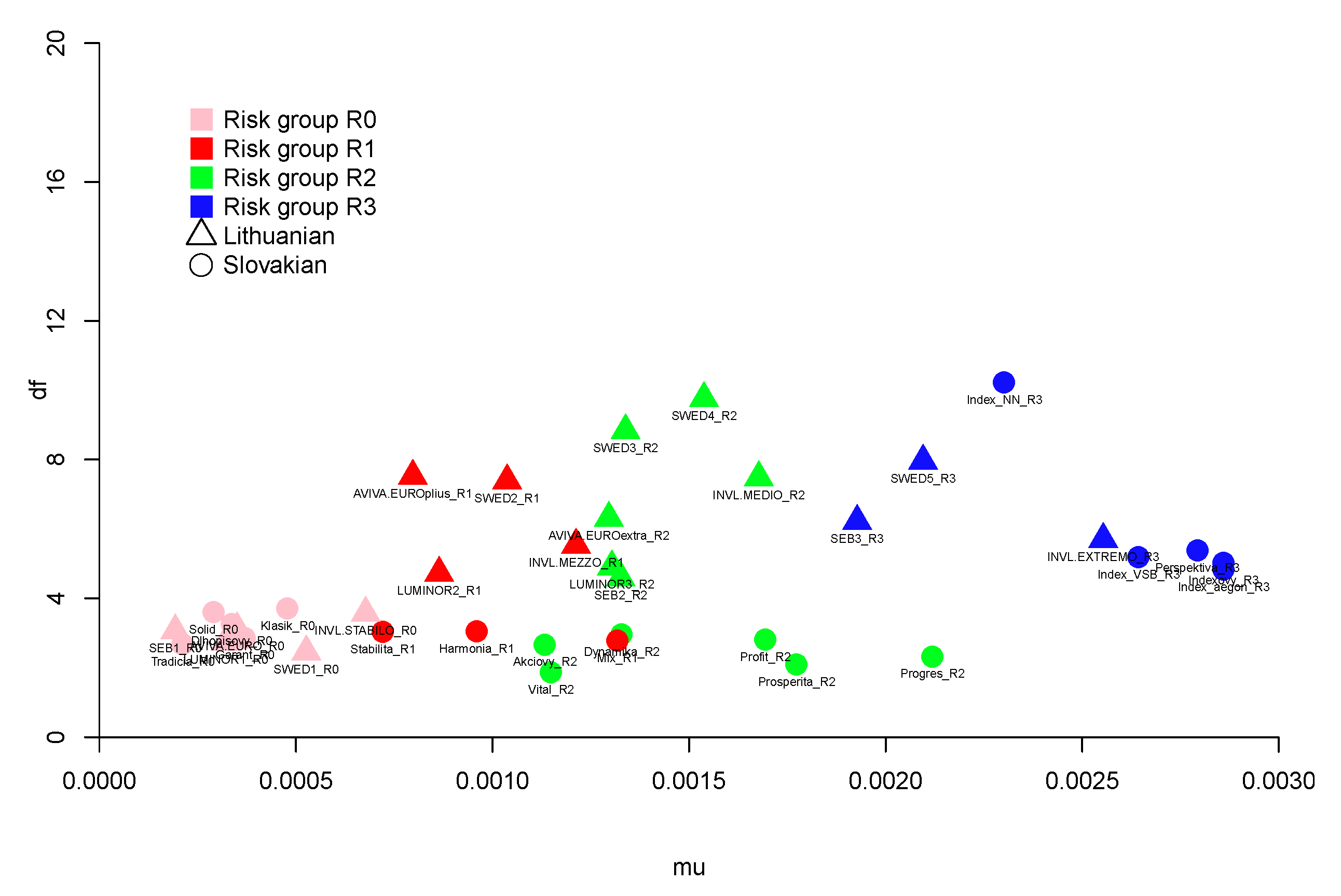
From the results in Figure 4, one conclusion can be drawn that less risky pension funds have substantially smaller student-t parameters $\nu$, which implies that these funds have heavier tails than the other ones. Surprisingly, the fund Vital in the R2 group has the smallest $\nu$ parameter among all funds, which indicates that the tails of the distribution will be heavy and theoretically the variance does not exist. However, it also has the worst fit according to the AD statistics. Moreover, the location parameter $\mu$ and scale parameter $\sigma$ are substantially larger for the R3 group, as expected.

Next, we describe the parameter estimation results for the hyperbolic and NIG distributions.

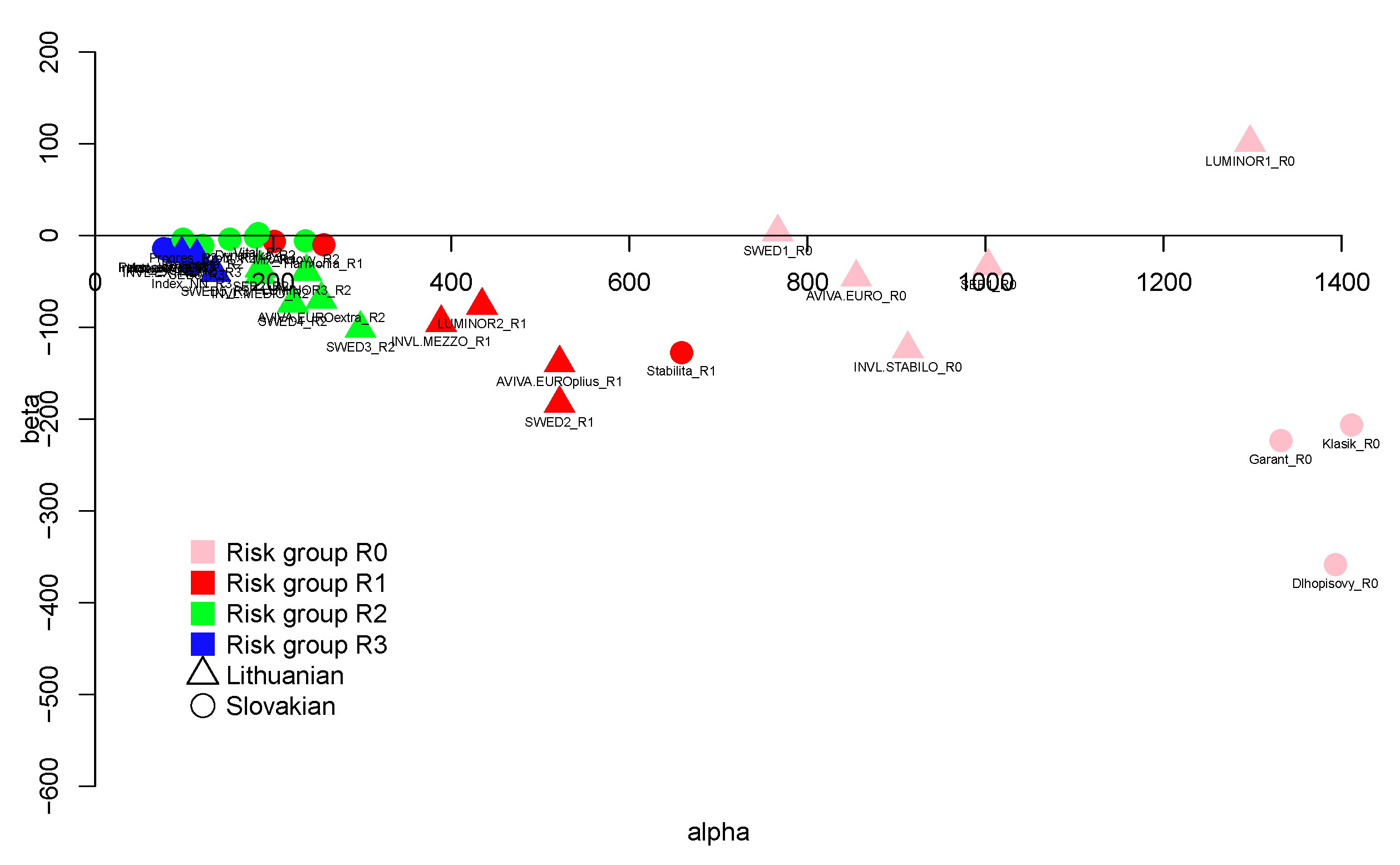
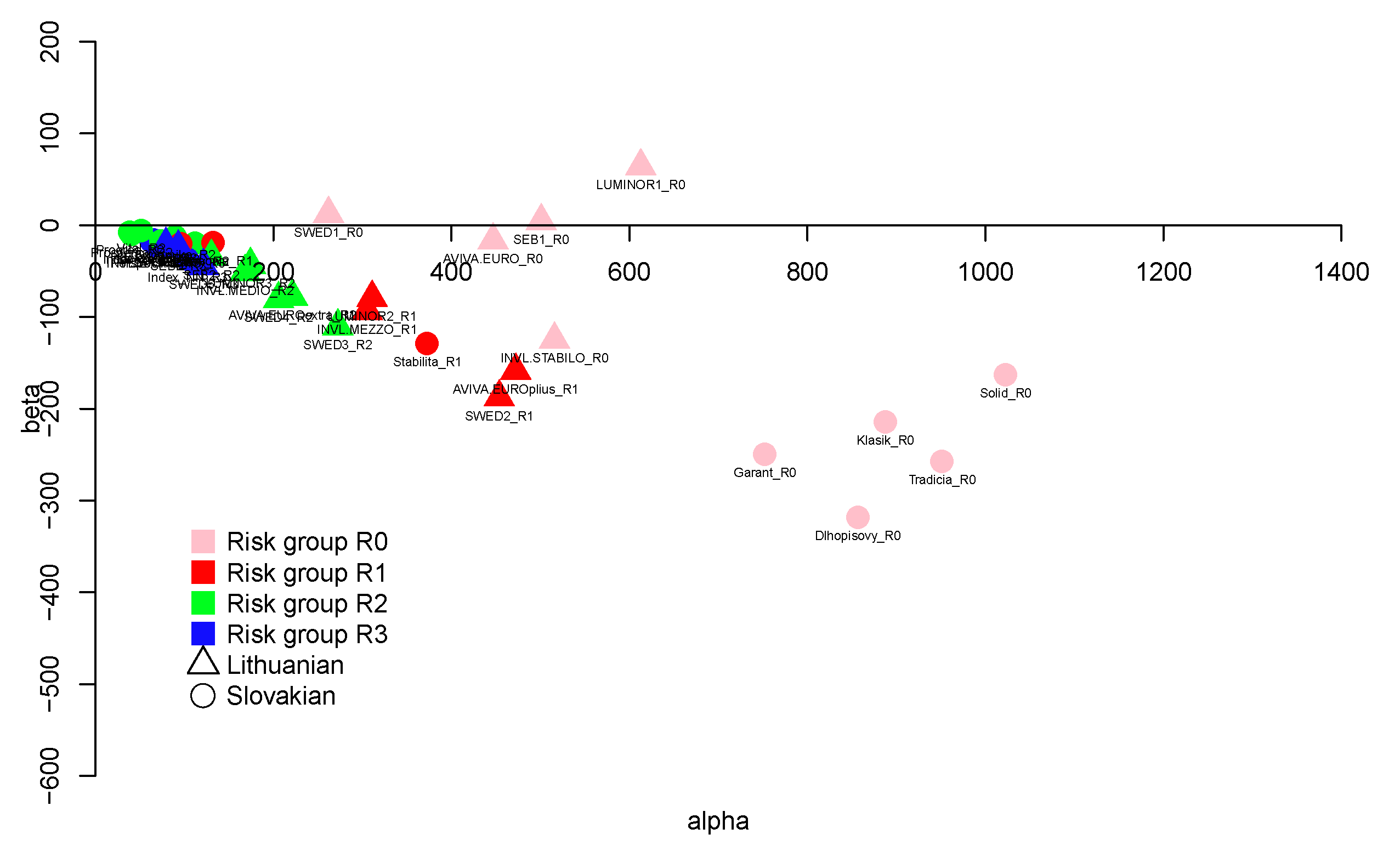
Figure 5 and Figure 6 clearly show that less risky funds have greater $\alpha$ parameter, while riskier funds have smaller $\alpha$ parameter. The hyperbolic distribution shows this result more clearly. However, such a result is not a surprise since greater $\alpha$ indicates a fatness of the tails similar to those observed in a normal distribution ($\alpha \to \infty$), while smaller values indicate heavier tails.

It is worth emphasising that the asymmetry (no mater what distribution is considered) is mainly negative, which indicates the negative tendency in return deviations. For both distributions, only the Lithuanian funds from the smallest risk Group R0 have positive $\beta$s. In particular, the Lithuanian funds LUMINOR1_R0 and SWED1_R0 are the only funds with positive asymmetries in both cases, while the Slovak fund Dlhopisovy_R0 has the most negative $\beta$,with a value close to $-400$.

3.3. Pairwise Stochastic Dominance based on Empirical Distribution

In this section, the stochastic dominance relations are analysed for the empirical weekly log-returns of each PF, with the equal probability $1/n$ assigned to each observed return. In order for the analyses to be interpretable over a wide range of risk preferences, we carried out experiments for all three criteria within the SD framework (FSD, SSD and TSD). The procedure involved making pairwise comparisons between any two funds, $X_i$ and $X_j$, $i,j=1,2,\dots 37$.

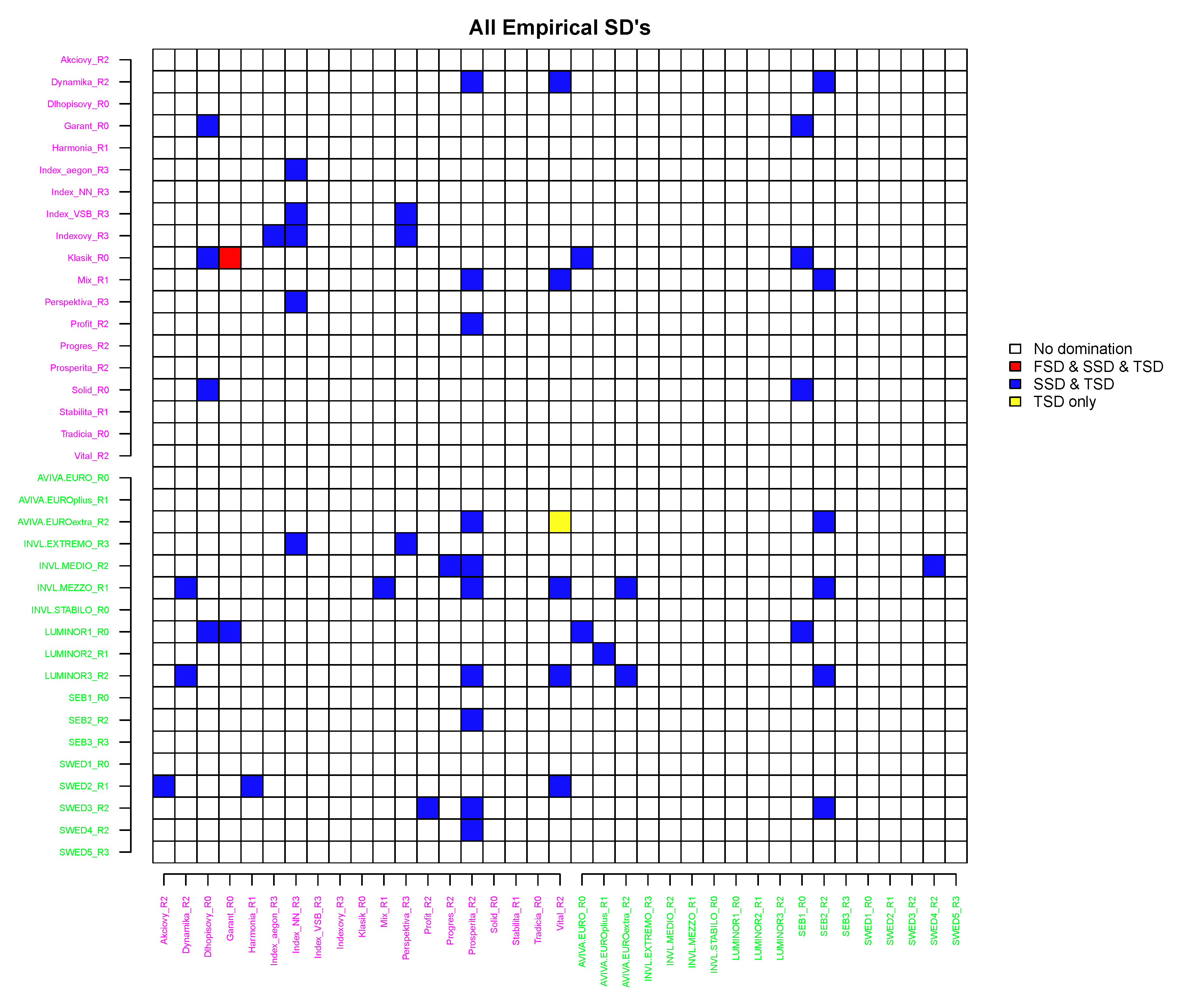
Figure 7 reports the results of the SD pairwise comparisons under all three dominance rules. Only those pairs for which there was found at least one SD relation are presented.

Figure 7 (and Figure 8, Figure 9 and Figure 10) should be understood as follows:

• The fund in the row dominates the fund in the column if the corresponding cell is not blank.
• If the cell is red, then FSD, SSD and TSD were found.
• If the cell is blue, then SSD and TSD were found.
• If the cell is yellow, then only TSD was observed.

Based on Theorem 1, if FSD is found, then SSD will definitely be found too. Accordingly, if SSD is found, then TSD will also be found.

It is of no surprise that only a single pair obeying FSD relation was identified (red cell in Figure 7) because this condition is very strict and related more to arbitrage. Hence, such case when Klasik_R0 dominates Garant_R0 under empirical FSD is rather the exception in our analysis, with no more FSD relations found under any parametric assumptions.

3.4. Pairwise Stochastic Dominance under a Student-t Distributional Assumption

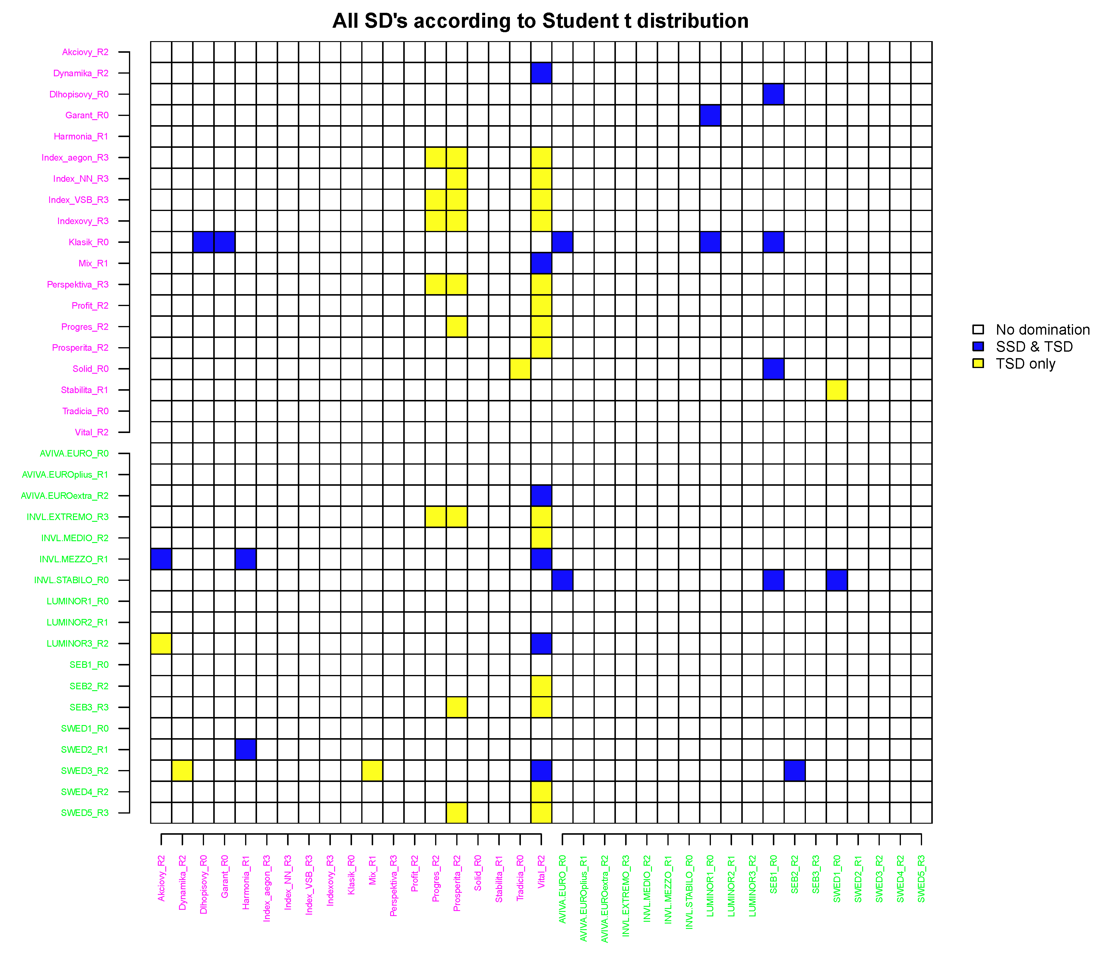
In Figure 8, we present the results based on the assumption that the returns follow student-t distribution.

To obtain SSD and TSD, we used numerical (correspondingly single or double) integration of the difference between the student-t cumulative distribution functions for each pair of funds, as given in Theorem 1. Figure 8 clearly shows that no FSD relation was found; moreover, SSD relations are also rarely observed. In particular, the fund Vital_R2 is significantly dominated by most of the remaining funds through a TSD relation and also in some funds using SSD rules. What is obviously specific to this fund is that it has the smallest parameter $\nu$ among all funds analysed, while the other parameters are not distinguishable comparing to other funds. On the whole, neither of the countries has an advantage in the number of clearly dominated or dominating funds, with the exception of Slovak fund Vital_R2.

3.5. Pairwise Stochastic Dominance under a Hyperbolic Distributional Assumption

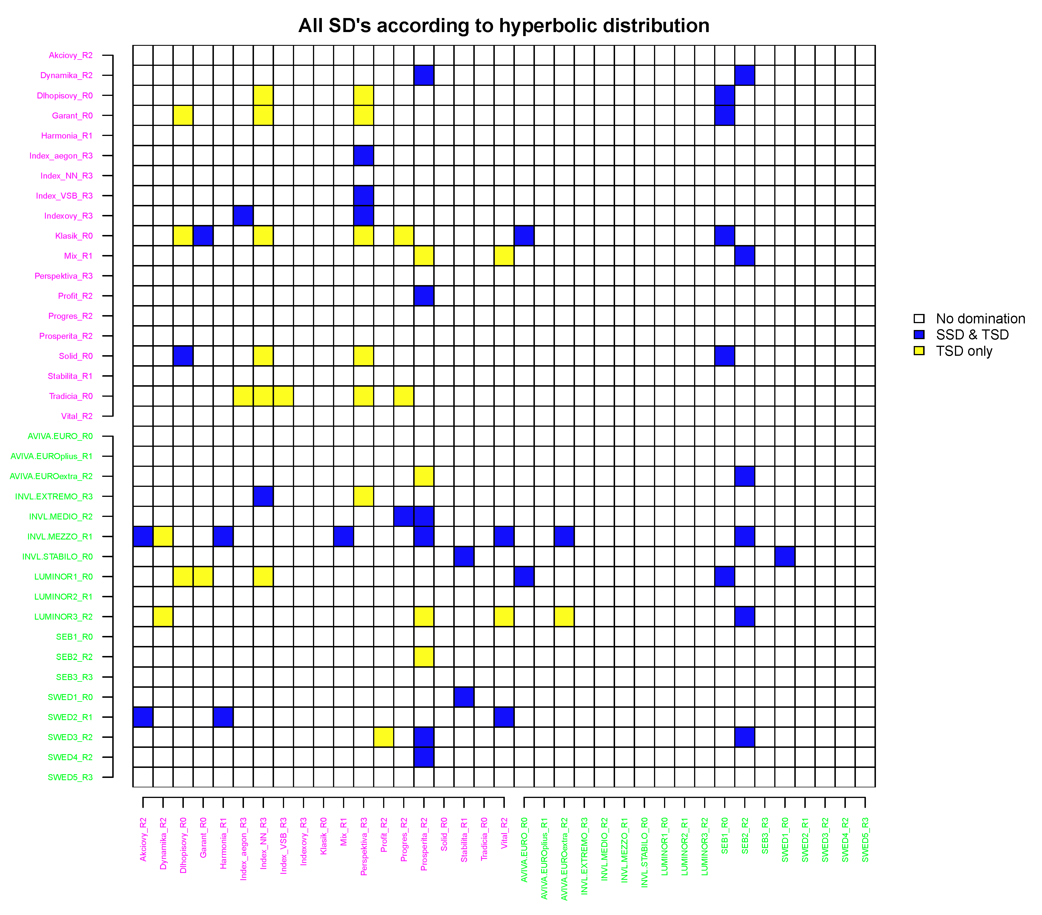
In Figure 9, we report on the pairwise SD comparison results for returns following a hyperbolic distribution.

No FSD relations were determined. However, under the hyperbolic distributional assumption, fewer Lithuanian funds are dominated than Slovak funds, i.e., only five Lithuanian funds are dominated, whereas nearly all Slovak funds are dominated by the TSD rule and, in some cases, the SSD rule. Notably, only a few funds do not dominate other funds in both countries.

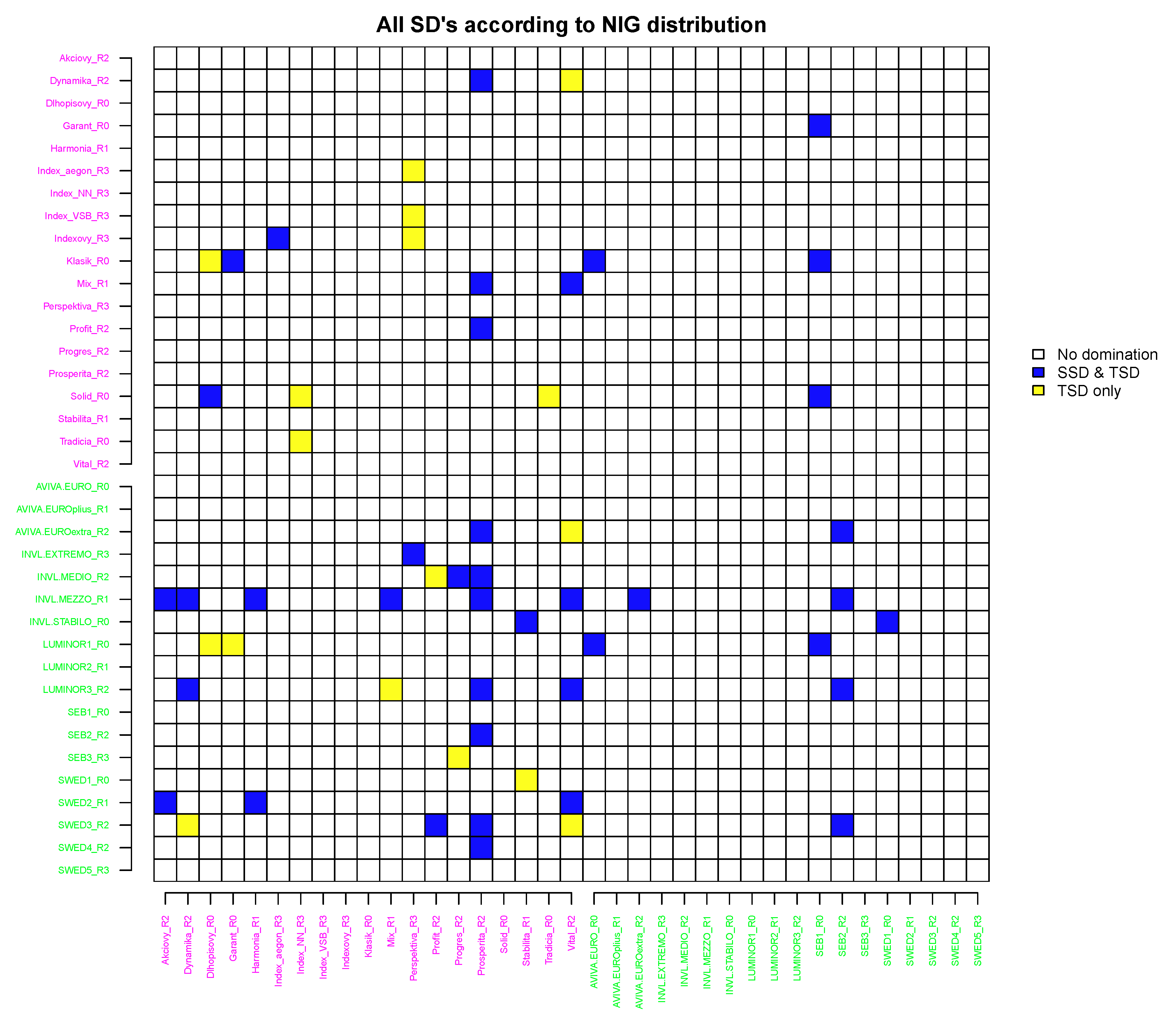
3.6. Pairwise Stochastic Dominance under a NIG Distributional Assumption

In Figure 10, the pairwise SD comparison results are demonstrated for returns following a NIG distribution.

The results in this case are similar to the results obtained under the hyperbolic distributional assumption; however, there are several differences. The SSD relations observed in the NIG case are mainly reflected under hyperbolic assumption too. However, in some cases, SSD${}_{\mathrm{NIG}}$ became TSD${}_{\mathrm{hyp}}$, e.g., the SSD relation for the pair Mix_R1 versus Prosperita_R2 became the TSD (the same holds for AVIVA.EUROextra_R2, LUMINOR3_R2 and SEB2_R2 to Prosperita_R2, etc). In a similar manner, the TSD in NIG case remained TSD under hyperbolic assumption. However, some TSDs observed in NIG case vanished in the hyperbolic case, e.g., Dynamika_R2 to Vital_R2. Furthermore, several TSDs appear in the hyperbolic case and are not observed in NIG case, e.g., Klasik_R0 to Index_NN_R3.

These results lead to the empirical conclusion that NIG SSD relation implies a hyperbolic SSD or TSD; however, the inverse does not hold. Summarising, stochastic dominance under the NIG assumption is more powerful than SD under the hyperbolic assumption; in practice, this finding means that different results will be obtained under these distributional assumptions and that both distributions must be assumed in decision making.

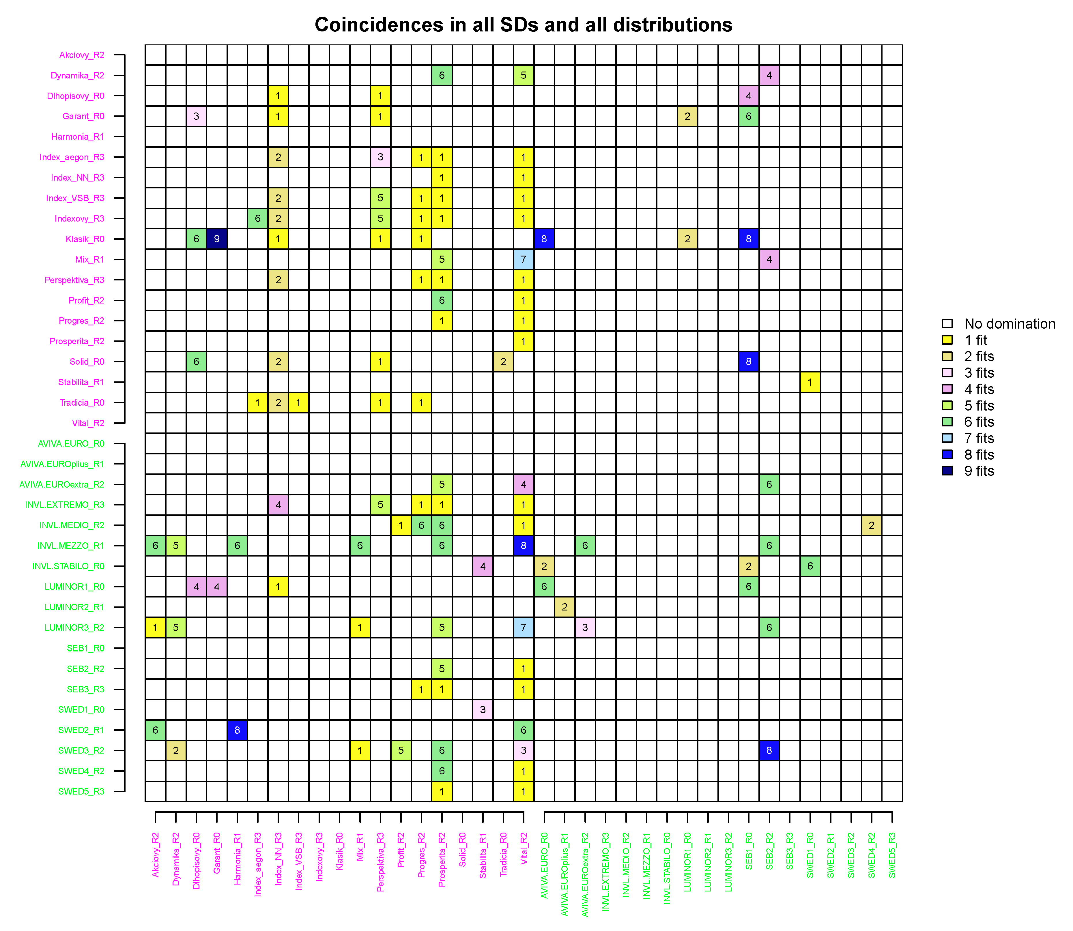
3.7. Overall Pairwise Stochastic Dominance Comparison Assuming all Considered Distributions

In this section, we explain the differences found in the SD pairwise comparisons when assuming the empirical, student-t, hyperbolic and NIG probability distributions for fund returns. Figure 11 summarises the results obtained in Section 3.3–Section 3.6 by presenting the matrix C used in Equation (2) and Step 5 from Section 2.7.

The entry $c_{ij}$ of matrix C and its corresponding value in Figure 11 identify how many times any kind of stochastic dominance was present for a particular pair i and j under the different assumptions used. There were a number of pairs, as seen in the figure, for which no SDs were identified at all. The greater the value of the entry is, the more times the SD relation was observed during the experiment. Therefore, with increasing value, a decision maker should become more confident that some type of SD relation exists for a particular pair. A value 1 means that a TSD was observed just once for pair $ij$ under all distributional assumptions. It is a bit more complicated to explain what values of 2–4 mean. For example, a value of 2 may mean that, for a pair $ij$, SSD and TSD relations were found under a single distributional assumption (e.g., Index_aegon_R3 and Index_NN_R3 in the empirical case) or two TSD relations were found under different distributional assumptions (e.g., Solid_R0 and Index_NN_R3 in the case of the NIG and hyperbolic distributions). Similar situations occur for the values of 3 and 4. The value $c_{ij}=4$ is the last case in which it is possible to observe only TSDs for the pairs involved. The value of 5 can be observed if at least one SSD and four TSDs are found for a pair $ij$. The value of 6 can be obtained for at least two SSDs and four TSDs. However, these cases mentioned are not of interest to the investor because the number of identified relations is less than median possible value and the of SD relation may be treated as weak. Moreover, there may be situations in which the SD was not observed under a single specific distribution, e.g., for the pair Dynamika_R2 and Prosperita_R2, no SD was identified under the student-t distributional assumption. Such issues cannot come up for seven and more identified relations. A value of 8 coincidences defines the benchmark for strong stochastic dominance because for a pair $ij$, all SSDs and all TSDs must be identified. For nine and more coincidences (in our case, for pair Klasik_R0 and Garant_R0), at least one FSD must be identified (in this case, an empirical FSD was observed), and the decision maker should be confident that the true stochastic dominance was found for a particular pair of funds.

To reveal the differences in SD comparison results, it is enough to compare Figure 8 and Figure 11, where matrices C and $C^{St}$ are presented. It can be clearly seen that mainly cases with entry values equal to 1 coincide if under the student-t distributional assumption only TSD was identified. Moreover, values of 7–9 in C coincide with SSD in $C^{St}$, which implies that the SSD under student-t distributional assumption might be a necessary condition for the existence of stronger SD relations. The difference in results is not very large when comparing hyperbolic SDs with NIG SDs. While the hyperbolic assumption allowed more SD pairs in general to be identified, the NIG distributional assumption had a higher rate of SSD compared to TSD.

3.8. Selection of the Most Preferable Pension Fund Based on Stochastic Dominance Ratio

In this section, the stochastic dominance ratio, which was proposed as a measure for identification of efficient funds and the most preferable PF (see Section 2.6), is estimated for all funds.

Table 4. The estimated stochastic dominance ratio.

Fund	Country	Fund Manager	${\mathit{D}}_{\mathit{i}}^{+}$	${\mathit{D}}_{\mathit{i}}^{-}$	${\mathit{R}}_{\mathit{i}}$	${\overline{\mathit{R}}}^{\mathbf{risk\; group}}$	${\overline{\mathit{R}}}^{*}$
Dlhopisovy_R0	Slovakia	AXA d.s.s.	6	19	−0.52	0.13	0.40
Garant_R0	Slovakia	Allianz-Slovenska	13	13	0
Klasik_R0	Slovakia	VUB Generali	36	0	1
Solid_R0	Slovakia	Aegon	19	0	1
Tradicia_R0	Slovakia	NN d.s.s.	6	2	0.5
AVIVA.EURO_R0	Lithuania	AVIVA	0	16	−1		−0.14
INVL.STABILO_R0	Lithuania	INVL	14	0	1
LUMINOR1_R0	Lithuania	LUMINOR	21	4	0.68
SEB1_R0	Lithuania	SEB	0	34	−1
SWED1_R0	Lithuania	Swedbank	3	7	−0.4
Harmonia_R1	Slovakia	NN d.s.s.	0	14	−1	0.08	−0.47
Mix_R1	Slovakia	VUB Generali	16	8	0.33
Stabilita_R1	Slovakia	DSS Postovej banky	1	7	−0.75
AVIVA.EUROplius_R1	Lithuania	AVIVA	0	2	−1		0.50
INVL.MEZZO_R1	Lithuania	INVL	49	0	1
LUMINOR2_R1	Lithuania	LUMINOR	2	0	1
SWED2_R1	Lithuania	Swedbank	20	0	1
Akciovy_R2	Slovakia	AXA d.s.s.	0	13	−1	−0.04	−0.59
Dynamika_R2	Slovakia	NN d.s.s.	15	12	0.11
Profit_R2	Slovakia	VUB Generali	7	6	0.08
Progres_R2	Slovakia	Allianz-Slovenska	2	14	−0.75
Prosperita_R2	Slovakia	DSS Postovej banky	1	65	−0.97
Vital_R2	Slovakia	Aegon	0	54	−1
AVIVA.EUROextra_R2	Lithuania	AVIVA	15	9	0.25		0.52
INVL.MEDIO_R2	Lithuania	INVL	16	0	1
LUMINOR3_R2	Lithuania	LUMINOR	28	0	1
SEB2_R2	Lithuania	SEB	6	34	−0.7
SWED3_R2	Lithuania	Swedbank	25	0	1
SWED4_R2	Lithuania	Swedbank	7	2	0.56
Index_aegon_R3	Slovakia	Aegon	8	7	0.07	0.43	0.08
Index_NN_R3	Slovakia	NN d.s.s.	2	20	−0.82
Index_VSB_R3	Slovakia	VUB Generali	10	1	0.82
Indexovy_R3	Slovakia	AXA d.s.s.	16	0	1
Perspektiva_R3	Slovakia	DSS Postovej banky	5	23	−0.64
INVL.EXTREMO_R3	Lithuania	INVL	12	0	1		1.00
SEB3_R3	Lithuania	SEB	3	0	1
SWED5_R3	Lithuania	Swedbank	2	0	1

Note. ${\overline{R}}^{*}={\overline{R}}^{\mathrm{country}|\mathrm{risk\; group}}$.

reports the $R_i$, $D_i^{+}$ and $D_i^{-}$ ratios for the Slovak and Lithuanian funds as well as the mean ratios per risk group and country.

According to the SD ratios, the risk-free (R0) funds Klasik_R0, Solid_R0 and INVL.STABILO_R0 are efficient because they are not dominated by other funds ($R_i=1$); moreover, the Slovak fund Klasik_R0 is the most preferable of those in this risk group because it dominates more funds than any other efficient fund from this risk group ($D_{Klasik}^{+}>D_{Solid}^{+}>D_{INVL.STABILO}^{+}$). The Lithuanian funds INVL.MEZZO_R1, LUMINOR2_R1 and SWED2_R1 from the group of low-risk (R1) funds are the only efficient funds, while the most preferable fund is INVL.MEZZO_R1 ($D_{INVL.MEZZO}^{+}>D_{SWED2}^{+}>D_{LUMINOR2}^{+}$). In the medium-risk (R2) group, the funds INVL.MEDIO_R2, LUMINOR3_R2 and SWED3_R2 are efficient, while LUMINOR3_R2 is the most preferable. The efficient funds in the high-risk group (R3) are Indexovy_R3, INVL.EXTREMO_R3, SEB3_R3 and SWED5_R3, with Indexovy_R3 being the most preferable fund.

As noted in the paragraph above, participants in the Slovakian and Lithuanian pension systems can select appropriately efficient funds from the risk-free and high-risk fund groups. However, there are no efficient Slovak funds in the low- or medium-risk groups. What should a Slovak participant do if his/her risk profile is somewhere in the middle, i.e., the participant prefers low- or medium-risk funds? We try to answer this question for each group separately.

In Group R1 (low-risk), there is only one fund with a positive SD ratio. Fund Mix_R1 is dominated by only three Lithuanian funds (see Figure 11) and dominates two Slovakian funds and one Lithuanian fund implying that this fund not so bad choice for participant who strongly prefers low-risk funds and lives in Slovakia.

In Group R2 (medium-risk), the two Slovakian funds Dynamika_R2 and Profit_R2 have positive SD ratios and potentially could be selected for investment. Both funds are dominated by just Lithuanian funds (see Figure 11). Moreover, they dominate the Slovakian funds Prosperita_R2 and Vital_R2 from the same risk group. However, Dynamika_R2 dominates more strongly (because $D_{Dynamika}^{+}>D_{Profit}^{+}$), and it dominates one additional Lithuanian fund, thus it should be selected as the most preferable Slovakian fund in this group.

If the participant has no preference in terms of a risk profile (group), then he should select an efficient fund anyway, because the SD ratio $R_i=1$ indicates that no fund exists anywhere that can dominate fund i under any circumstances. The most preferable fund in Slovakia, according to Table 4, is Klasik_R0 ($R_{Klasik}=1$ and $D_{Klasik}^{+}=36$ is maximal among Slovakian funds), and the most preferable Lithuanian fund is INVL.MEZZO_R1 ($R_{INVL.MEZZO}=1$ and $D_{INVL.MEZZO}^{+}=49$).

Additionally, Table 4 presents two mean ratios ${\overline{R}}^{\mathrm{risk\; group}}$ and ${\overline{R}}^{\mathrm{country}|\mathrm{risk\; group}}$ for the comparison of risk groups, in general, and then, more deeply, within countries as well.

Firstly, the averaging is done within a particular risk group. The ratio ${\overline{R}}^{\mathrm{risk\; group}}$ shows how good funds from a particular risk group are. For example, a participant in the pension system can easily compare funds included in risk Group R0 with funds from other risk groups. In our experiment, the risk-free funds (R0) did slightly better than the low-risk funds (R1) because ${\overline{R}}^{R0}=0.13>{\overline{R}}^{R1}=0.08$ and outperform medium-risk funds (R2), for which ${\overline{R}}^{R2}=-0.04$, which indicates that this group of funds is more SD-dominated than -preferred. However, it is no surprise that high-risk funds (R3) are more preferable (on average) than any other group because the average SD ratio for the group is equal to $0.43$.

Next, the averaging is done within particular risk groups in Lithuania and Slovakia separately using ${\overline{R}}^{\mathrm{country}|\mathrm{risk\; group}}$. From the last column, it is easy to deduce that the funds operating in Lithuania are more preferable that those operating in Slovakia, with the exception of risk-free funds. The average SD ratio for the R0 group of Slovak funds is $0.4$, while, for Lithuanian funds, it is $-0.14$. Such a difference indicates that, on average, risk-free Slovak funds are better managed than Lithuanian funds. It is worth emphasising that Lithuanian low-risk (R1) funds are much more preferable than Slovakian R1 funds since their estimated average SD ratio ${\overline{R}}^{R1|LT}=0.50$ is much greater than ${\overline{R}}^{R1|SK}=-0.47$. Notably, the most preferable fund overall, INVL.MEZZO_R1, is from this group, with $\overline{R}=1$, and its $D^{+}$ equal to 49, while the most preferable Slovak fund, Klasik_R0, has $D^{+}=36$. The greatest difference between two countries in average SD ratio is observed in Group R2, where ${\overline{R}}^{R2|LT}=0.52$ and ${\overline{R}}^{R2|SK}=-0.59$. The low SD ratios of Slovak funds indicates a subpar average performance compared to other funds.

Finally, we examine the outstanding group of high-risk funds (R3), where smallest average SD ratio for the Slovak funds is 0.08. Moreover, the Lithuanian funds in this group have an average ${\overline{R}}^{R3|LT}=1$, which indicates that all funds in this subgroup are efficient.

In the same manner, we can identify the “worst” funds and their risk groups in each country. Moreover, if necessary or a participant would like to, it is easy to compare entire pension systems between countries or pension fund managers. The latter comparison is useful when selecting a PF management company for an entire career. Such behaviour is observed in Lithuania, where participants are rather passive and do not react to changes in the financial market.

4. Discussion

In the current paper, we examine a case study focusing on the comparison of pension funds within risk groups and within countries over a certain time period. According to the proposed dominance ratio, the most preferable pension funds are found in the Lithuanian high-risk fund group (R3), while the least preferable are in the Slovakian medium-risk fund group (R2).

To put it another way, the estimated SD ratio can be also used to evaluate the PF managers. For example, among Lithuanian companies, the absolute top manager is “Invalda INVL Group”. All pension funds managed by this company resulted in SD ratio of 1, which means that the company can suggest efficient fund in every risk group. Conversely, the funds managed by SEB bank have both negative and positive SD ratios, depending on risk group selected. Within the Slovak pension system, no most preferable manager was found, but, for example, all funds, namely, Klasik_R0, Mix_R1, Profit_R2 and Index_VSB_R3, managed by “VÚB Generali d.s.s.” had positive SD ratios. Notably, all funds, namely, Stabilita_R1, Prosperita_R2 and Perspektiva_R3, managed by “DSS Poštovej banky d.s.s.” were estimated to have negative ratios. This point is important when a participant is not planning to change the pension fund manager in future but only a risk group within the same manager. In practise, the participants often have some default choices, in either risk group or PF manager. The newly developed stochastic dominance ratio not only helps a participant to select the best fund from a default group but also allows them to compare the default group with the other groups, perhaps providing important information about the quality of the default choices.

The interesting question is how the efficiency of PFs based on newly derived SD ratio corresponds with the estimated risk and performance measures. On the basis of risk groups defined by the stock share in a portfolio, it is possible to observe that the high-risk Group R3 is the most efficient group, which can be explained by the contained risk and comparatively high mean returns exhibited by the funds within Group R3. Considering Group R2 and especially the Slovak PFs within this group, the negative SD ratios could be related to the estimated risk measures, which are more in line with those observed for Group R3 and are not outweighed by a sufficiently high mean. On the other hand, if we consider the risk-free funds in the R0 group, the Lithuanian funds had negative and lower SD ratios than the Slovak funds. Even though the risk estimates are similar between the countries, the mean value observed for the Lithuanian funds is smaller.

5. Conclusions

The current paper presents decision making rules based on the three most commonly used stochastic dominance relations, i.e., FSD, SSD and TSD, for the selection of a private pension fund. The approach was demonstrated for the PFs operating in Lithuania and Slovakia, but it is not limited to these countries and can be applied for the selection of an investment fund when there are many alternatives and different possible risk profiles for the decision maker. Stochastic dominance allows the dominated (or inefficient) funds to be identified. Since the decision rules based on SD could be integrated into a robo-advisory solution, the sensitivity of the rules to the distributional assumption (empirical, student-t, hyperbolic and NIG) is investigated in this paper.

Furthermore, a new stochastic dominance ratio and corresponding decision-making rules are proposed. This ratio allows assets (pension funds) to be ranked while taking into account all the distributional and SD assumptions considered to be equally important for decision makers. Moreover, the averaged ratio allows funds assigned to different risk groups based on the stock shares in the portfolio to be compared.

As an alternative to the approach presented in the current paper, weaker types of stochastic dominance such as decreasing absolute risk aversion stochastic dominance, increasing relative risk aversion (see [47]) or almost stochastic dominance (see, e.g., [48] of various orders) could be considered; however, tractable formulations exist only for discrete distributions.

The probability distributions considered in this paper were mainly from the family of semi-heavy-tailed distributions; however, the results of our data analysis indicate that some funds have shape parameters that are indicative of fat-tailed distributions ($\alpha$ or $\nu$ is rather small). Therefore, the possible inclusion of fat-tailed distributions could be analysed in future research.

One of the basic features of PF selection in Lithuania and Slovakia is that every participant can choose only one second-pillar pension fund, that is, no diversification is allowed. If at least limited diversification were possible, then notion of portfolio efficiency with respect to stochastic dominance could be employed [49]. Moreover, one could formulate portfolio selection models maximising the dominance ratio.Alternatively, a pre-selection of pension funds based on the dominance ratio could be undertaken before applying some of the usual portfolio selection models. In this case, only funds with $R=1$ could be used as base assets. Finally, dynamic (multi-stage) portfolio (or asset-liability) management models [5,8,27] could be extended in order to find the optimal investment strategy for a participant. These models could either maximise the dominance ratio or at least keep it reasonably high (only portfolios with sufficiently high dominance ratios would be feasible).

References

- OECD. Pensions at a Glance; Pension-System Typology; OECD iLibrary: Paris, France, 2006. [Google Scholar] [CrossRef]
- Carone, G.; Eckefeldt, P.; Giamboni, L.; Laine, V.; Sumner, S.P. Pension Reforms in the EU since the Early 2000’s: Achievements and Challenges Ahead; Technical Report; European Commission Directorate—General for Economic and Financial Affairs; Publications Office of the European Union: Luxembourg, 2016. [Google Scholar]
- World Bank. The World Bank Pension Conceptual Framework; Technical Report; World Bank: Washington, DC, USA, 2008. [Google Scholar]
- Lusardi, A. Financial literacy and the need for financial education: Evidence and implications. Swiss J. Econ. Stat. 2019, 155, 1. [Google Scholar] [CrossRef] [Green Version]
- Kabašinskas, A.; Maggioni, F.; Šutienė, K.; Valakevičius, E. A multistage risk-averse stochastic programming model for personal savings accrual: The evidence from Lithuania. Ann. Oper. Res. 2019, 279, 43–70. [Google Scholar] [CrossRef]
- Strumskis, M.; Balkevičius, A. Pension fund participants and fund managing company shareholder relations in Lithuania second pillar pension funds. Intellect. Econ. 2016, 10, 1–12. [Google Scholar] [CrossRef] [Green Version]
- Kabašinskas, A.; Šutienė, K.; Kopa, M.; Valakevičius, E. The risk–return profile of Lithuanian private pension funds. Econ. Res.-Ekon. Istraživanja 2017, 30, 1611–1630. [Google Scholar] [CrossRef] [Green Version]
- Moriggia, V.; Kopa, M.; Vitali, S. Pension fund management with hedging derivatives, stochastic dominance and nodal contamination. Omega 2019, 87, 127–141. [Google Scholar] [CrossRef]
- Zenios, S.; Ziemba, W. (Eds.) Handbook of Asset and Liability Management: Applications and Case Studies; North-Holland: San Diego, CA, USA, 2008. [Google Scholar]
- Kumar, R. Cases on Pension Funds. In Strategies of Banks and Other Financial Institutions; Kumar, R., Ed.; Academic Press: San Diego, CA, USA, 2014; pp. 463–483. [Google Scholar] [CrossRef]
- Kusy, M.I.; Ziemba, W. A Bank Asset and Liability Management Model. Oper. Res. 1986, 34, 356–376. [Google Scholar] [CrossRef] [Green Version]
- Geyer, A.; Ziemba, W.T. The Innovest Austrian pension fund financial planning model InnoALM. Oper. Res. 2008, 56, 797–810. [Google Scholar] [CrossRef] [Green Version]
- Dupačová, J.; Polívka, J. Asset-Liability Management for Czech Pension Funds Using Stochastic Programming. Ann. Oper. Res. 2009, 165, 5–28. [Google Scholar] [CrossRef] [Green Version]
- Klein Haneveld, W.K.; Streutker, M.H.; van der Vlerk, M.H. An ALM Model for Pension Funds Using Integrated Chance Constraints. Ann. Oper. Res. 2010, 177, 47–62. [Google Scholar] [CrossRef] [Green Version]
- De Oliveira, A.; Filomena, T.; Perlin, M.; Lejeune, M.; de Macedo, G. A Multistage Stochastic Programming Asset-Liability Management Model: An Application to the Brazilian Pension Fund Industry. Optim. Eng. 2017, 18, 349–368. [Google Scholar] [CrossRef] [Green Version]
- Alwohaibi, M.; Roman, D. ALM models based on second order stochastic dominance. Comput. Manag. Sci. 2018, 15, 187–211. [Google Scholar] [CrossRef] [Green Version]
- Hinz, R.; Rudolph, H.P.; Antolin, P.; Yermo, J. Evaluating the Financial Performance of Pension Funds; Technical Report; World Bank: Washington, DC, USA, 2010. [Google Scholar]
- Kupčík, P.; Gottwald, P. The Return-risk Performance of Selected Pension Fund in OECD with Focus on the Czech Pension System. Acta Univ. Agric. Silvic. Mendel. Brun. 2016, 64, 1981–1988. [Google Scholar] [CrossRef] [Green Version]
- Matek, P.; Lukač, M.; Repač, V. Performance Appraisal of Croatian Mandatory Pension Funds; Effectus—Working Paper Series 0004; Effectus—University College for Law and Finance: Zagreb, Croatia, 2015. [Google Scholar]
- Ehrgott, M. Multicriteria Optimization; Springer: Berlin/Heidelberg, Germany, 2005. [Google Scholar]
- Barros, C.; Garcia, M. Performance Evaluation of Pension Funds Management Companies with Data Envelopment Analysis. Risk Manag. Insur. Rev. 2006, 9, 165–188. [Google Scholar] [CrossRef]
- Levy, H. Stochastic Dominance. Investment Decision Making under Uncertainty; Springer International Publishing: Switzerland, Germany, 2016. [Google Scholar]
- Rockafellar, R.; Uryasev, S. Optimization of conditional value-at-risk. J. Risk 2000, 2, 21–42. [Google Scholar] [CrossRef] [Green Version]
- Farinelli, S.; Ferreira, M.; Rossello, D.; Thoeny, M.; Tibiletti, L. Beyond Sharpe ratio: Optimal asset allocation using different performance ratios. J. Bank. Financ. 2008, 32, 2057–2063. [Google Scholar] [CrossRef]
- Rachev, S.T.; Stoyanov, S.V.; Fabozzi, F. Advanced Stochastic Models, Risk Assessment, and Portfolio Optimization: The Ideal Risk, Uncertainty, and Performance Measures; Wiley: New York, NY, USA, 2008. [Google Scholar]
- Sortino, F.A.; Price, L.N. Performance Measurement in a Downside Risk Framework. J. Investig. 1994, 3, 59–64. [Google Scholar] [CrossRef]
- Kopa, M.; Moriggia, V.; Vitali, S. Individual optimal pension allocation under stochastic dominance constraints. Ann. Oper. Res. 2018, 260, 255–291. [Google Scholar] [CrossRef]
- Levy, H. Stochastic Dominance and Expected Utility: Survey and Analysis. Manag. Sci. 1992, 38, 555–593. [Google Scholar] [CrossRef]
- Post, T.; Kopa, M. Portfolio Choice Based on Third-Degree Stochastic Dominance. Manag. Sci. 2017, 63, 3381–3392. [Google Scholar] [CrossRef] [Green Version]
- Stoyanov, S.V.; Rachev, S.T.; Racheva-Yotova, B.; Fabozzi, F.J. Fat-Tailed Models for Risk Estimation. J. Portf. Manag. 2011, 37, 107–117. [Google Scholar] [CrossRef] [Green Version]
- Sheikh, A.Z.; Qiao, H. Non-normality of market returns: A framework for asset allocation decision making. J. Altern. Invest. Winter 2010, 12, 8–35. [Google Scholar] [CrossRef] [Green Version]
- Esch, D. Non-normality facts and fallacies. J. Invest. Manag. 2010, 8, 49–61. [Google Scholar]
- Rachev, S.; Racheva-Iotova, B.; Stoyanov, S. Capturing fat tails. Risk Mag. 2010, 23, 72–77. [Google Scholar]
- Kabasinskas, A.; Sakalauskas, L.; Sun, E.W.; Belovas, I. Mixed-Stable Models for Analyzing High-Frequency Financial Data. J. Comput. Anal. Appl. 2012, 14, 1210–1226. [Google Scholar]
- Barndorff-Nielsen, O.E.O.E.; Mikosch, T.; Resnick, S.I. Levy Processes: Theory and Applications; Birkhauser: Boston, MA, USA, 2001. [Google Scholar]
- Eberlein, E.; Keller, U. Hyperbolic Distributions in Finance. Bernoulli 1995, 1, 281–299. [Google Scholar] [CrossRef]
- Socgnia, V.K.; Wilcox, D. A Comparison of Generalized Hyperbolic Distribution Models for Equity Returns. J. Appl. Math. 2014, 2014, 263465. [Google Scholar] [CrossRef]
- Huang, C.K.; Chinhamu, K.; Huang, C.S.; Hammujuddy, J. Generalized Hyperbolic Distributions and Value-at-Risk Estimation for the South African Mining Index. Int. Bus. Econ. Res. J. (IBER) 2014, 13, 319–328. [Google Scholar] [CrossRef] [Green Version]
- Stefan, J.S.; Voicu, D. Pension Savings: The Real Return, 2019 ed.; Technical Report; Public Interest Non- Governmental Organisation Better Finance: Brussels, Belgium, 2019. [Google Scholar]
- Petronis, T.; Dičpinigaitienė, V. Review of Lithuania’s 2nd and 3rd Pillar Pension Funds and of the Market of Collective Investment Undertakings in 2018; Technical Report; Lithuanian Bank: Vilnius, Lithuania, 2019. (In Lithuanian) [Google Scholar]
- Mestan, M.; Šebo, J.; Kralik, I. How are 1bis pension pillar funds performing? A cross-country analysis. In European Financial Systems 2017: Proceedings of the 14th International Scientific Conference; Masaryk University: Brno, Czech Republic, 2017; pp. 52–59. [Google Scholar]
- Hammerstein, E.A.F. Generalized Hyperbolic Distributions: Theory and Applications to CDO Pricing. Ph.D. Thesis, Albert-Ludwigs-Universitat Freiburg, Breisgau, Germany, 2010. [Google Scholar]
- Uryasev, S.; Rockafellar, R.T. Conditional Value-at-Risk: Optimization Approach. In Stochastic Optimization: Algorithms and Applications; Springer: Boston, MA, USA, 2001; pp. 411–435. [Google Scholar] [CrossRef]
- Sharpe, W.F. Capital Asset Prices: A Theory of Market Equilibrium under Conditions of Risk. J. Financ. 1964, 19, 425–442. [Google Scholar]
- Menn, C.; Fabozzi, F.J.; Rachev, S. Fat-Tailed and Skewed Asset Return Distributions: Implications for Risk Management, Portfolio Selection, and Option Pricing; John Wiley & Sons Inc.: Hoboken, NJ, USA, 2005. [Google Scholar]
- Anderson, T.W.; Darling, D.A. Asymptotic Theory of Certain “Goodness of Fit” Criteria Based on Stochastic Processes. Ann. Math. Statist. 1952, 23, 193–212. [Google Scholar] [CrossRef]
- Post, T.; Fang, Y.; Kopa, M. Linear Tests for Decreasing Absolute Risk Aversion Stochastic Dominance. Manag. Sci. 2015, 61, 1615–1629. [Google Scholar] [CrossRef]
- Leshno, M.; Levy, H. Preferred by “All” and Preferred by “Most” Decision Makers: Almost Stochastic Dominance. Manag. Sci. 2002, 48, 1074–1085. [Google Scholar] [CrossRef] [Green Version]
- Post, T.; Kopa, M. General linear formulations of stochastic dominance criteria. Eur. J. Oper. Res. 2013, 230, 321–332. [Google Scholar] [CrossRef]
Figure 1.
CDF of student-t distribution depending on degrees of freedom.
Figure 2.
CDF of Hyperbolic distribution against and .
Figure 3.
CDF of normal-inverse Gaussian distribution against and .
Figure 4.
Scatter plot of estimates of location and degrees of freedom parameters of scaled student-t distribution for Slovak and Lithuanian pension funds.
Figure 5.
Scatter plot of estimates of shape and asymmetry parameters of hyperbolic distribution for Slovak and Lithuanian pension funds.
Figure 6.
Scatter plot of estimates of shape and asymmetry parameters of NIG distribution for Slovak and Lithuanian pension funds.
Figure 7.
Empirical SD relations for all PFs.
Figure 8.
SD relations for all PFs assuming student-t distribution.
Figure 9.
SD relations for all PFs assuming hyperbolic distribution.
Figure 10.
SD relations for all PFs assuming NIG distribution.
Figure 11.
SD for all PFs assuming all considered distributions.