1. Introduction
Industry 4.0 requires not only fully connected factories, but also a fully automated production process. As Facchini et al. [
1] explained, this new age in industry provides an opportunity to optimize and reorganize all company structures. Therefore, this new era also requires new methods and tools, such as mobile robots.
These mobile robots, known as automated guided vehicles (AGVs) or autonomous mobile robots (AMRs) are being implemented to automate logistics and handmade production processes. As Teso-Fz-Betoño et al. [
2] noted, the differences between these technologies rest in how much they can do. An AGV simply follows a magnetic field, while AMRs have the ability to interact with the area and adapt to each trajectory when an obstacle appears due to the use of different sensors and algorithms to modify each navigation instance.
Normally, in industry, an AMR will use LiDAR technology to move around the factory. Catapang et al. [
3] studied the implementation of 2D LiDAR for obstacle detection. Moreover, it is possible to implement 3D LiDAR to recognize pedestrians (see Wang et al. [
4]).
Nevertheless, vision algorithms are increasing in popularity in the field of navigation because computer vision ensures the competitiveness of manufacturing enterprises by offering adaptability to various industries (see Lass et al. [
5]). Algorithms such us machine learning (ML) and deep learning (DL) have been the most frequently implemented in recent years. These algorithms are based on the mathematics that Deisenorth et al. [
6] demonstrated in their book, which expresses machine learning problems such as density estimation with Gaussian mixture models, classification with support vector machines, etc.
Image detection is one of the techniques that uses ML or DL (see Cheng et al. [
7]). However, the differences between these techniques lie in the amount of data needed to train the computer to identify the object in the image. DL requires abundant spatial and contextual information to improve its interpretation of the object and also increase its performance, as noted by Tian et al. [
8].
In addition to object detection, semantic segmentation is another method that uses DL. This technique is a key topic. Minae et al. [
9] summarized the sematic segmentation situation by describing the most widely used datasets, comparing each dataset’s performance, and discussing promising future research directions. Li et al. [
10] compiled different structures to realize the actual situation of sematic segmentation. A segmentation network’s output uses several binary masks to segment the input image into different classes. Therefore, some situations require solving a binary optimization problem (see Minaee et al. [
11]).
Cheng et al. [
12] described several different neural networks, such as the hybrid dilated convolution U-Net (HDCUNet), which combines U-Net and a hybrid dilated convolution (HDC) network. Convolutional neural networks (CNNs) are also implemented in segmentation processes, according to Marchal et al. [
13]. Additionally, Doan et al. [
14] proposed a residual network to segment different street objects, such as cars, pedestrians, etc. Mask-RCNN was proposed by Kowalewski [
15] to build a map and detect objects in indoor surroundings, while Chen et al. [
16] implemented a CNN for direct mapping using vision. However, Bersan et al. [
17] used sematic segmentation to implement more information into the map, such us corridor doors. Koval et al. [
18] presented a classical technique that does not use DL or ML but has a high calculation speed because the applied mathematical equations require less powerful hardware.
According to Bengio et al. [
19], developing an artificial intelligence (AI) that is less dependent on engineering features, like edge detection, color segmentation, etc., is crucial to the progress of this type of intelligence. Moreover, a fully convolutional neural (FCN) network with transfer learning was proposed by Huang et al. [
20]. Further, a pretrained FCN can make a decision by analyzing an accuracy comparison, as shown by Raghu et al. [
21].
Thus, to develop autonomous indoor driving, not only is it important to verify that the AI can be implemented, but it is also essential to verify the existence of any AI for outdoor navigation. For example, the automobile industry is developing these technologies to implement level 5 autonomous driving [
22]. Gao et al. [
23] developed robust line detection by implementing hybrid deep architectures using a combination of a CNN and a recurrent neural network (RNN). Sun et al. [
24] developed a novel sequence-based deep neural network to predict the trajectory. Pohlen et al. [
25] combined multi-scale context with pixel-level accuracy by adopting two processing streams: One stream carries information at the full image resolution, enabling precise adherence to segment boundaries. The other stream undergoes a sequence of pooling operations to obtain robust features for recognition. Chen et al. [
26], however, showcased another type of semantic segmentation with neural networks by implementing an atrous spatial pyramid pooling in an image cascade network (AtICNet). A thermal image was adopted on a deep neural network to include extra information. Sun et al. [
27] proposed a novel encoder–decoder architecture network to segment urban scenes. It is essential to determine the navigable area for mobile robots, and Wang et al. [
28] presented a novel concept for wheelchairs: By adopting an RGB-D camera, the CNN segments the drivable area. Moreover, an automatic labeling system was developed. Badrinarayanan et al. [
29] introduced a SegNet to engage in semantic segmentation under different scenarios. A previously developed dual attention network (DANet) integrated local features with their global dependencies (see Fu et al. [
30]). Zhang et al. [
31] presented a neural network based on enhancing feature fusion to bridge the gap between low-level and high-level features by significantly improving segmentation quality. Yeboah et al. [
32] explained how to develop a CNN for indoor autonomous navigation by implementing transfer learning.
The main goal of the present study is to develop indoor navigation for an AMR by implementing a CNN that segments the image to determine the navigable zone and calculates the steering and speed commands by applying different mathematical operations. In this way, the AMR can move in the corridor without any collisions by taking images from a monocular camera, processing the information via the CNN, and commanding the AMR motors.
2. Materials and Methods
This article presents an indoor navigation for an AMR. In this section, the development of the algorithms is explained. In the first subsection, the CNN mathematical equations are presented. In the second subsection, the neural network training will be explained, and in the third subsection, the path calculation and motion are analyzed. The last subsection presents the AMR that is used for this experiment.
2.1. Convolutional Neural Network
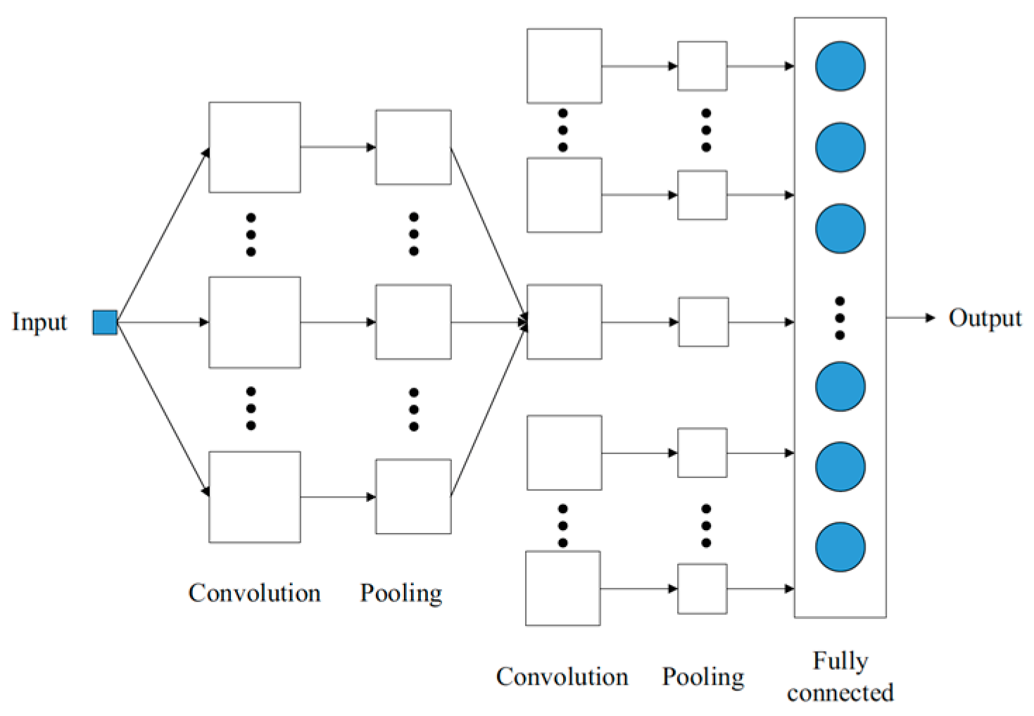
CNN is the most popular type of deep neural network architecture [
33]. Usually, the network consists of an input layer, one or more convolution and pooling layers, a fully connected layer, and an output layer, as shown in
Figure 1.
The input layer has a dimension of 240*240*3. Therefore, the input data consist of three matrices with dimensions of 240*240, and each matrix corresponds to the red, green, blue (RGB) scale, which contains the value of each pixel from 0 to 255. The zero value is the black color, and 255 is white in gray scale.
The convolution layer is the specific structure of the CNN. Depending on the configuration, this layer could be different and execute a filter that convolves with a local region from the input image. The convolution equation is given as Equation (1), where
represents the matrix filter, and
is the bias parameter:
where
is the input layer,
is the result,
is initialized with a small matrix (such as 3*3 or 5*5), and
b is the BIAS parameter. This matrix is adjusted during the training process until it minimizes the CNN output error. Furthermore, the output of this network uses a nonlinear activation function. Equations (2)–(4) represent the most common functions—Sigmoid, Tanh, and ReLU respectively. ReLU is usually chosen because it has a faster convergence rate.
The pooling layer progressively decreases the spatial size of the representation to reduce the number of parameters and computations in the network. The pooling layer operates on each feature map independently, as shown in Equation (5), where
is the filter used to reduce the image to analyze the background and texture.
The last one is a fully connected layer that provides a way to learn non-linear combinations of high-level features represented by the output of the convolutional layer. The fully connected layer learns a possibly non-linear function in that space. Considering this basic theory of the CNN, there are different possible architectures, as noted by Canziani et al. [
34]. The results of the experiment demonstrated the power of all networks by concluding that VGG and Alexnet are oversized, while Efficient Net (ENet), ResNet-18, and GoogleNet offer better performance. ResNet-18 is an efficient network that is well suited for applications with limited processing resources. Moreover, the chosen indoor scenario has less changeability than a street scenario. Therefore, the data set could be smaller, as could the CNN’s complexity. ResNet-18 has all the necessary qualities for use in this indoor scenario. He et al. [
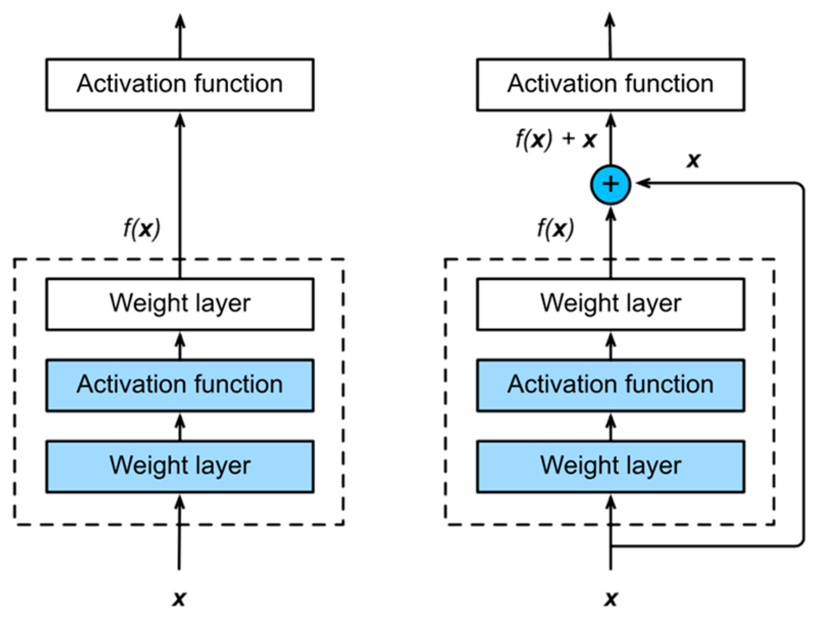
35] demonstrated that the ResNet model differs from the CNN mathematic model. Thus, we next describe the residual network function.
Figure 2 illustrates the spatial structure of a ResNet.
is used for optimum mapping and is obtained by a network learning algorithm. This kind of architecture can avoid the gradient evanishing effect because the features learned by a layer are directly applied to the outlier layer, as shown in
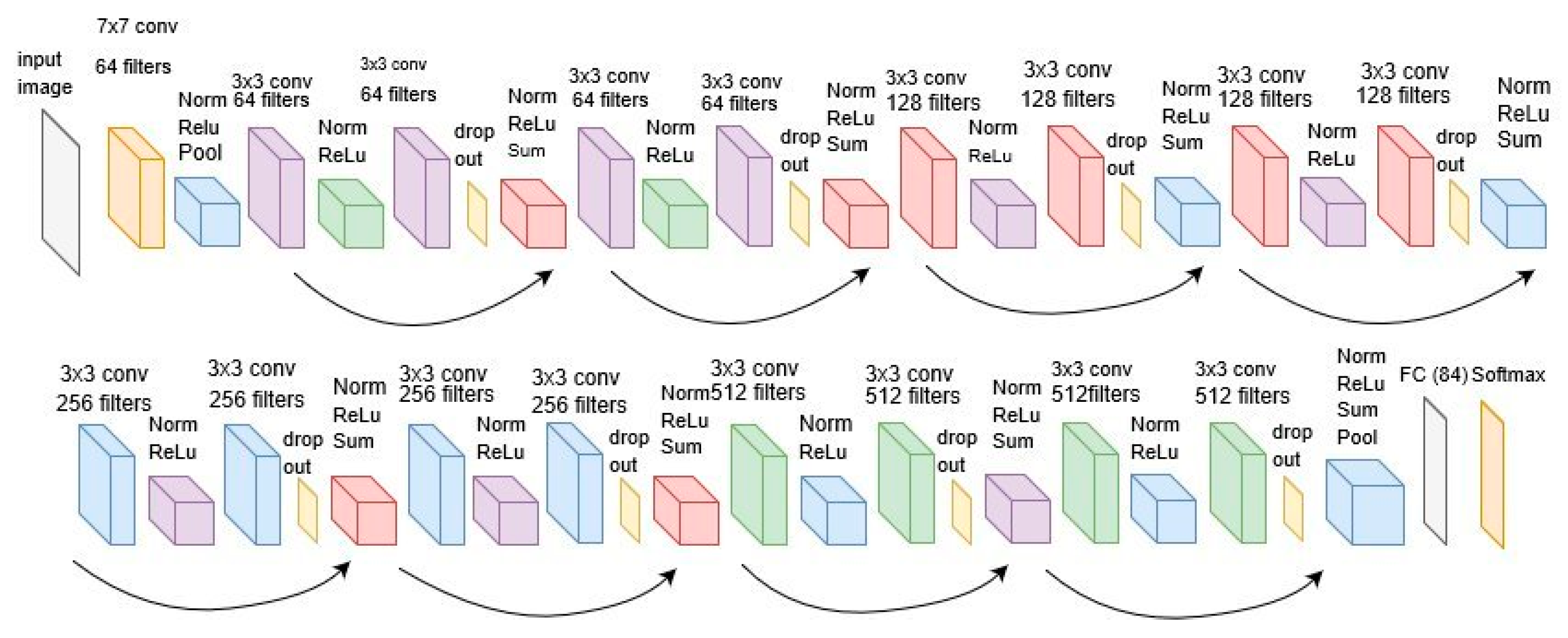
Figure 2. The aim of this explanation is to introduce convolutional neural networks and not to produce a mathematical model, as it is important to understand the basic concepts to improve the results of the learning process. Thus, the ResNet-18 configuration is presented in
Figure 3 with a total of 18 layers. These layers are composed of a convolutional layer and a ReLU layer or of a convolutional layer, a drop out layer, and ReLU. The last layer is always SoftMax.
It is assumed that the drop out layer tries to prevent overfitting and that SoftMax is a function that limits the output of the function into a range of 0–1. This consideration allows the output to be interpreted directly as a probability (see Equation (6)).
After discussing the basic theory of CNN and ResNet-18, we will analyze the equation that calculates the path and how it will move the AMR.
2.2. ResNet-18 Learning Process
There are three steps in the learning process: data acquisition, data preparation, and training. In the current work, the first action consists of taking photos of the surroundings where the AMR will move.
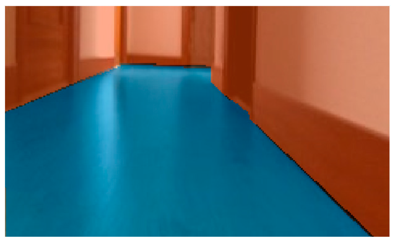
The second step consists of labelling the image and is crucial for sematic segmentation. In this particular case, semantic segmentation distinguishes the two labels: the blue ones are the floor, and the orange ones are all the elements that are not considered the floor, such as walls, obstacles, etc. The orange label is the wall. In addition, both labels are considered pixel labels, and this technique consists of assigning a label to each pixel (see
Figure 4). In other words, a binary mask is created manually for each label and for each image. Henceforth, this mask represents only a segment of the image that corresponds to the label.
In total, 391 photos are labeled. These photos were obtained by recording the scenario several times while the AMR was moving. From this video, some frames were selected as arbitrary to prepare the data set. Moreover, 80% of the images are used in learning process; 19% for validating and the rest for testing. The learning data were improved by achieving data augmentation with the reflection, X, and Y translation functions. The image rotation was not considered because the AMR move on the X and Y plane.
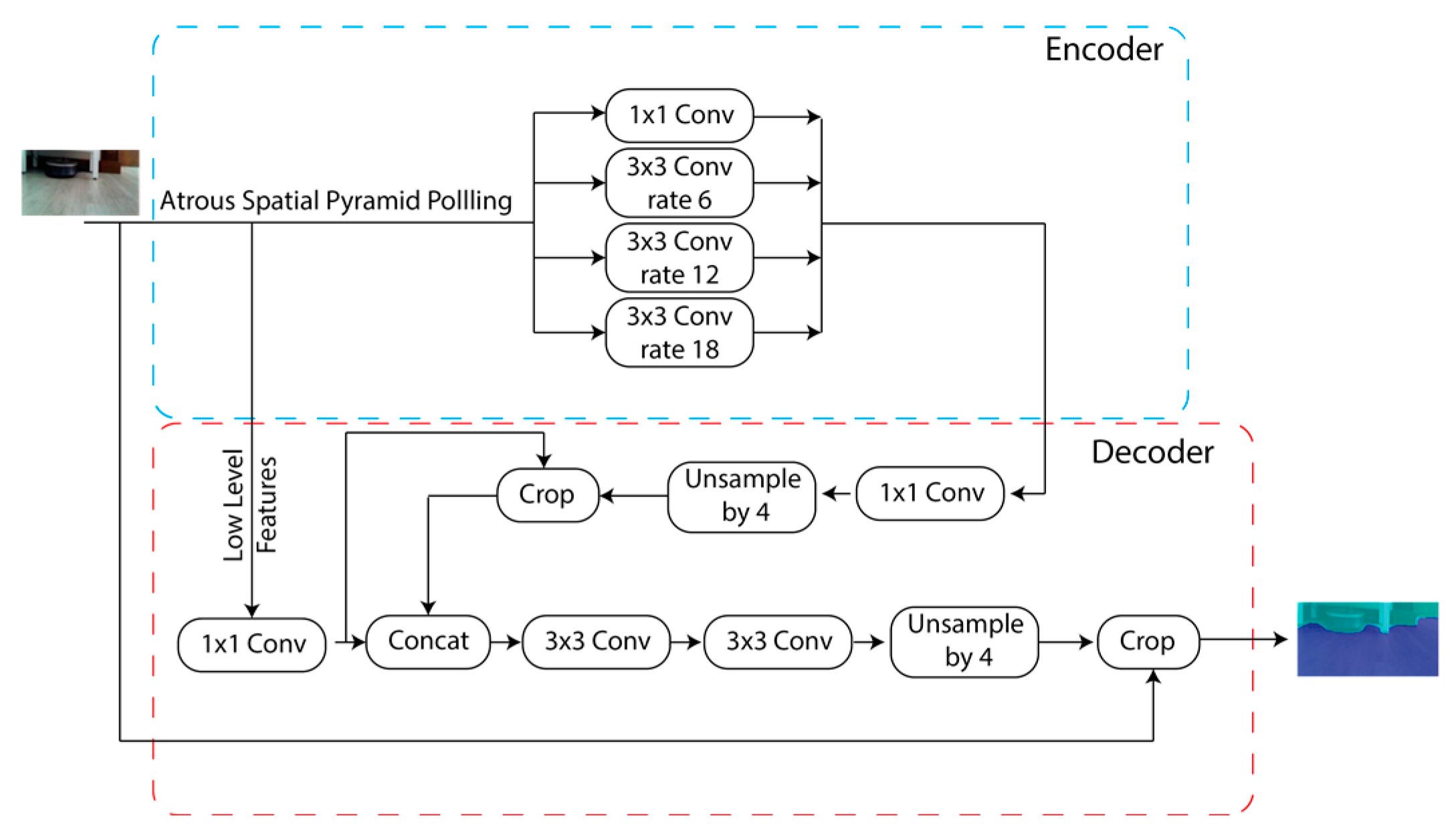
ResNet-18 is a classification network that has to be modified to realize semantic segmentation. The network uses encoder–decoder architecture, dilated convolutions, and skip connections to segment images by adopting the DeepLabV3+ technique [
36]. The encoder module gradually reduces the feature maps to obtain more semantic information by utilizing Atrous convolution at multiple scales. Therefore, Atrous convolution controls the density of the encoder. However, the decoder gradually recovers the spatial information. In
Figure 5, the network layer structure is shown.
Moreover, the training parameters for the neural network are presented in
Table 1 and are not optimized. In the current work, semantic segmentation information is used to safely navigate the AMR in a specific indoor scenario.
The set of options for training a network use a stochastic gradient descent with momentum (sgdm) (see Equation (7)). “L” is the loss function,
is the gradient with respect to the weight, and
is the learning rate. The learning rate is reduced by a factor of 0.1 every 5 epochs.
The maximum number of epochs for training is set as 100 with 10 used as a mini-batch for the observations in each iteration. The initial learning rate used for training is 0.003. If the learning rate is too low, then training takes a long time. If the learning rate is too high, then training might achieve a suboptimal result or diverge. L2 Regularization sets the factor of the layer learnable parameter. The gradient threshold method controls the gradient of a learnable parameter, and if it is larger than the gradient threshold, the gradient is scaled to equal the L2 norm. The validation frequency value is the number of iterations between evaluations of the validation metrics. The validation patience value is the number of times that the loss on the validation set is larger than or equal to the previously smallest loss before the network training finishes. Shuffle is set at every epoch to shuffle the training data before each training epoch and to shuffle the validation data before each network validation. The piecewise learn rate schedule settings method updates the learning rate for a certain number of epochs by multiplying them by a certain factor. The learn rate drop factor name-value pair argument specifies the value of this factor. The learn rate drop period name-value pair argument is used to specify the number of epochs between multiplications.
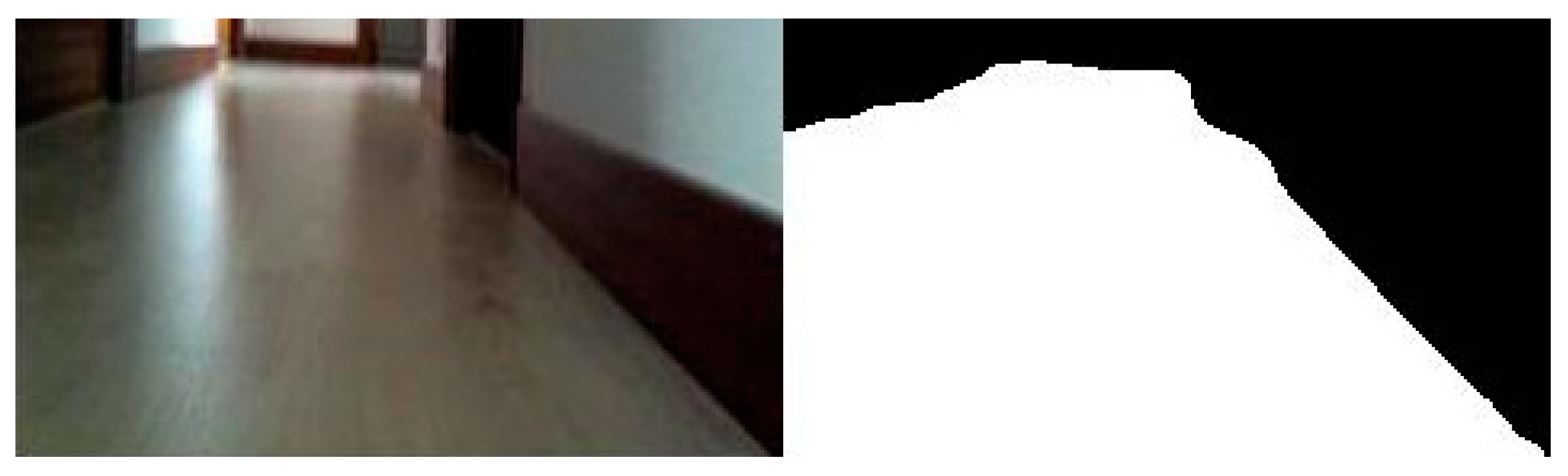
The total training time with a Quadro P1000 was about 16 min. The results of the semantic segmentation after retraining the network are presented in
Figure 6, where the solution is a mask that divides the floor from the rest of elements.
However, after developing this neural network, the AMR cannot move without path calculations and motion estimations. Thus, in the next subsection, both cases are studied to implement the necessary intelligence in the robot for it to move around this area.
2.3. Path Calculation and Motion
The path calculation and motion are divided into two parts. The first section uses the ResNet-18 classification results to calculate the middle path from the free space. The second one involves the development of the motor control.
The neural network result is represented by a matrix with a dimension of 240*240*1 (see Equation (8)). To measure the free space, the matrix has to be decomposed into horizontal vectors (see Equation (9)), and by counting the consecutive white pixels of each vector, the dimension can be estimated. In some situations, there is more than one vacant space. Therefore, the maximum measurement is chosen to calculate the middle point of the free space.
Moreover, all
are equal to 0 or 255, where 0 indicates black pixels and 255 indicates white pixels. Afterwards,
is classified by discriminating the black pixels (see Equation (10)):
After considering where the white pixels are located, we can measure how many pixels are consecutive. This expression is represented by Equation (11):
where
and
are the vectors used to measure the start and end pixels. Therefore,
is a vector whose dimension varies depending on how many free spaces are identified. Afterwards, in some cases, there is an obstacle in the middle of the freeway. Thus, the free space is divided into two sections, and
. In this situation, the AMR has to avoid an obstacle by moving to the maximum vacant space (see Equation (14)):
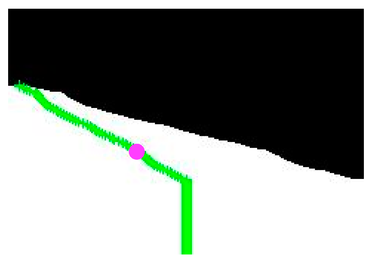
After selecting the best measurement, the middle point is calculated by considering the position of the start and end pixel locations based on the best measurement (see Equation (15)). All results are collected in the middle vector to represent them as an image (see
Figure 7).
The magenta circle in
Figure 7 represents the controlling point. In order to use all the estimated paths to enable motion control, a single point is chosen. This is done to determine if semantic segmentation can be used for indoor navigation. This single point changes its location depending on the conditions. In the end, the algorithms calculate the path conditions from
to
, which is shown at the bottoms of the images and assumes the worst case by analyzing the distance between the middle point and the x = 120 px vertical line (see Equation (16)):
where Steering represents the value in px of the worst case, and the place variable includes the “
g” value for when the maximum value is detected. This steering value is transformed into a percentage value by considering the limitation indicated by Equations (17) and (18):
is determined as
. Therefore, this Steer value modifies the wheel speed according to the sign of the
. When the sign is positive, the purple circle is located on the left side, and the right wheel reduces its speed as illustrated in
Figure 7. However, when the purple circle is on the opposite side, the other wheel needs to decrease its velocity, as revealed by Equations (19)–(21):
where Vel = 0.5 is a fixed value that is half of the duty cycle that can be sent to the motors. Additionally, a security function is implemented for situations where there is not enough space to modify the robot’s trajectory (see Equation (22)). The
is set with a
value.
Once the intelligence that controls the AMR was developed, the mobile robot itself was tested.
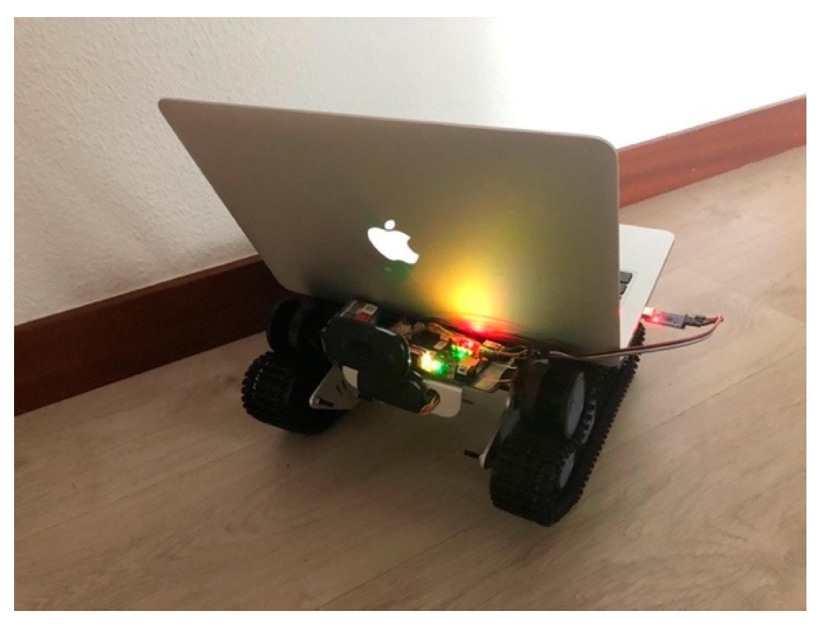
2.4. The Autonomous Mobile Robot
This AMR was developed using a tank chassis, a BeagleBone Blue, a webcam, and a laptop. The tank chassis has two 9 Volt DC motors to move the tracks and is controlled via BeagleBone Blue. The BeagleBone Blue is an all-in-one Linux-based minicomputer for robotics with an AM335x 1 GHz ARM® Cortex-A8 processor and 512 MB DDR3 RAM. Moreover, the main program for this platform was developed with python. Communication between the laptop and the minicomputer is realized via a serial connection. The neural network is located in the laptop and is executed in a 2.9 GHz Intel Core i7 with 8 Gb of ram. These results are conditioned by the laptop’s capacity. Finally, the webcam is connected to the laptop, where the sematic segmentation is executed.
Figure 8 illustrates the AMR.
3. Results and Discussion
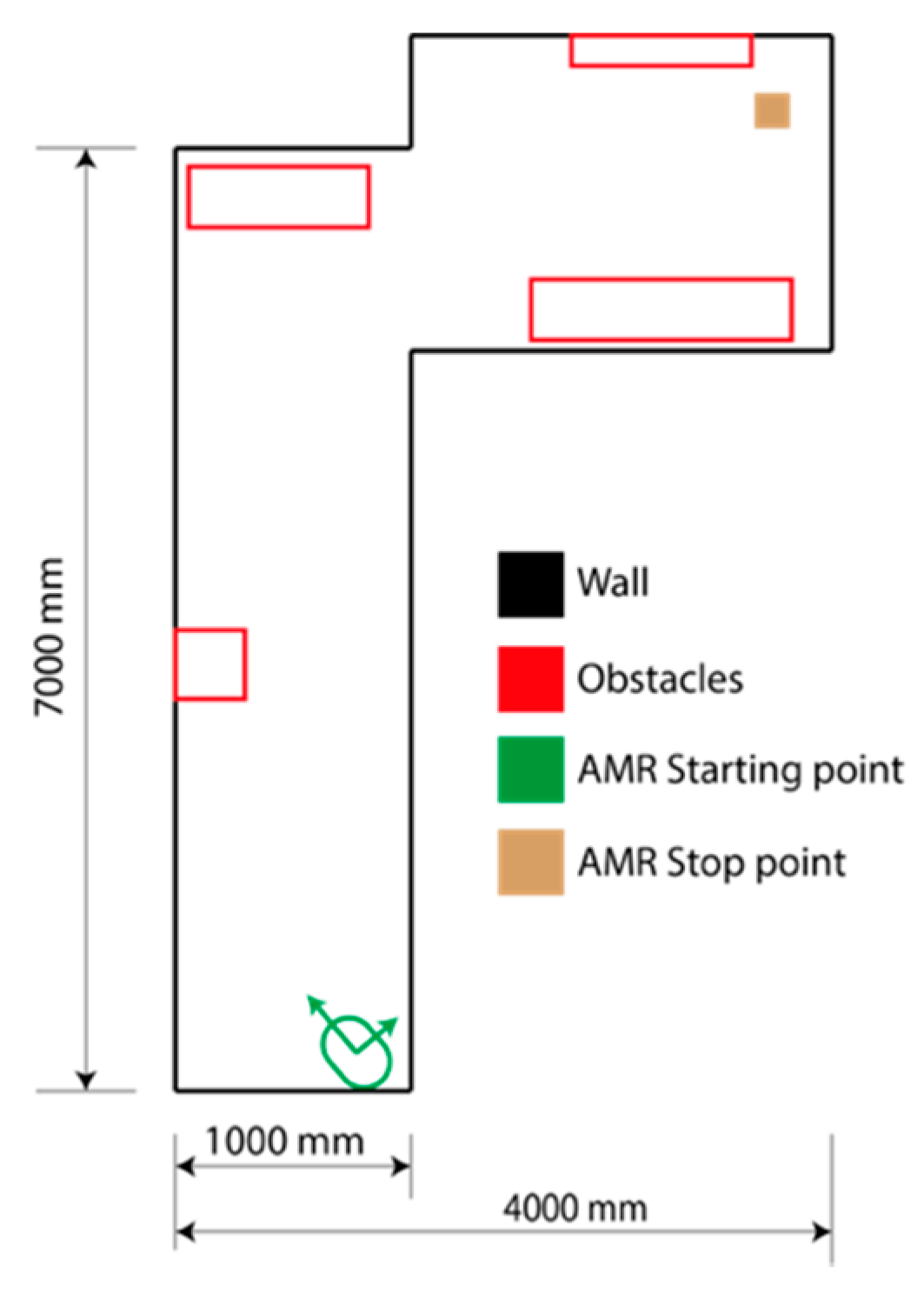
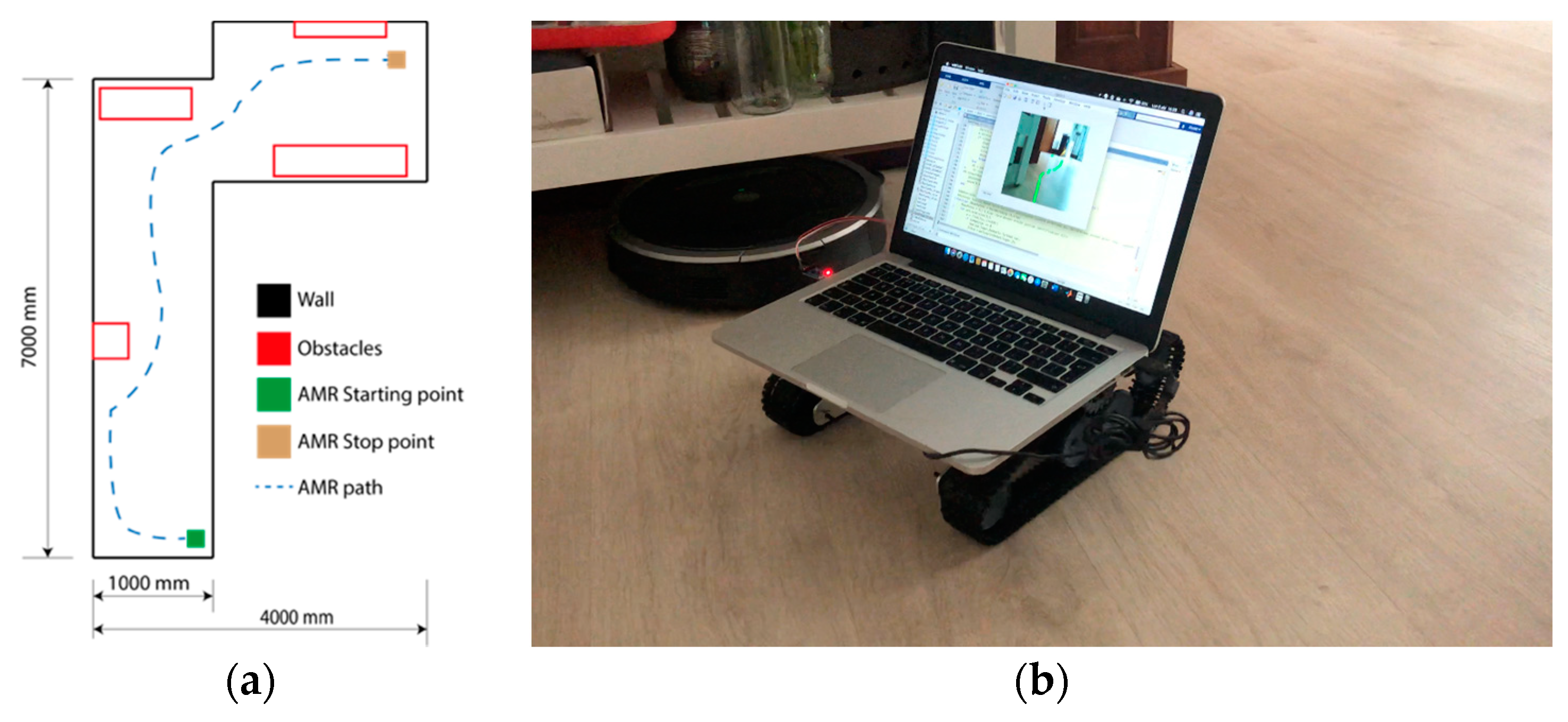
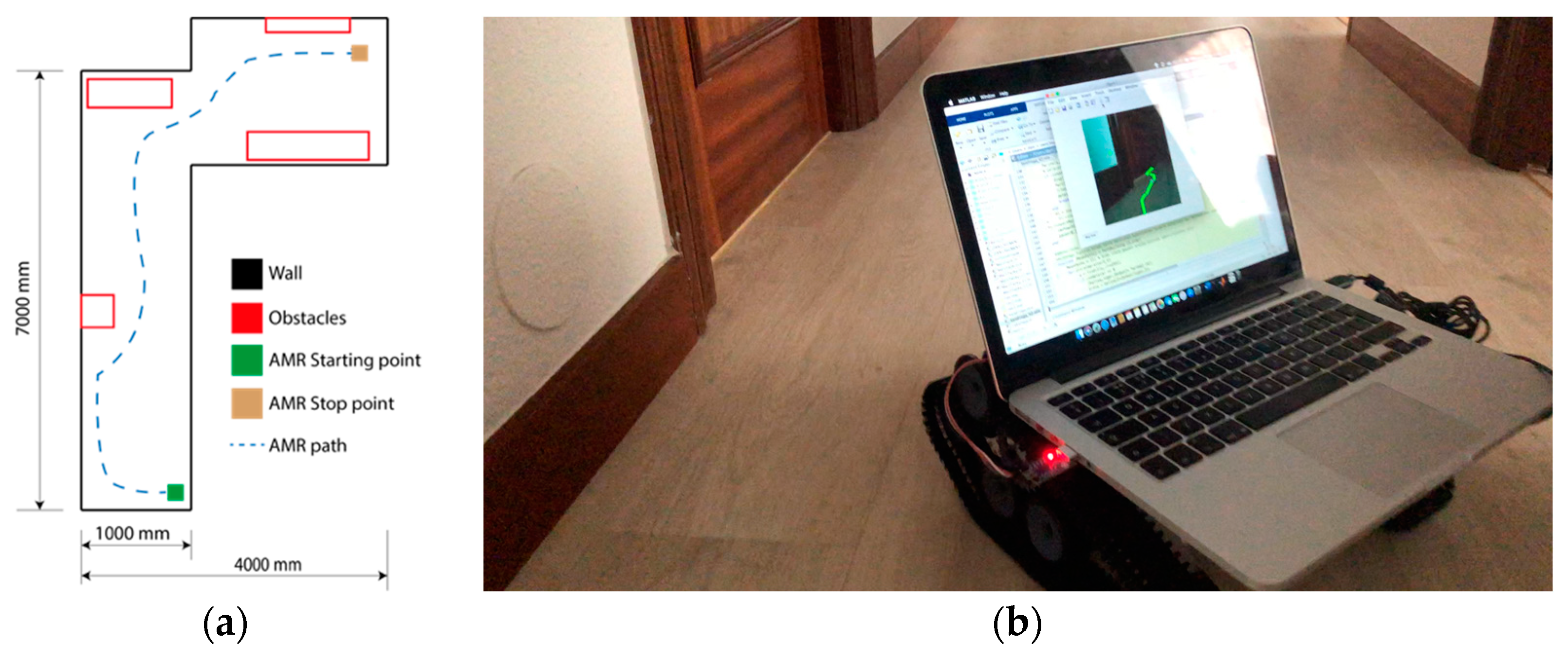
Real execution was performed in order to study indoor navigation. This scenario includes a corridor with several obstacles, such as walls, furniture, boxes, etc.
Figure 9 illustrates a sketch of the scenario and the robot’s starting position.
The results are determined by comparing the speed command for each motor and controlling the execution time of the neural network. Moreover, some pictures are captured to understand the calculated path.
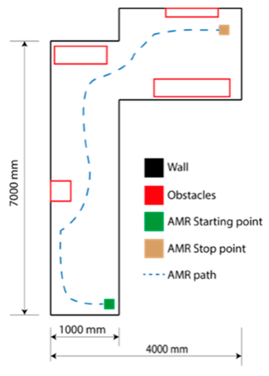
Figure 10 represents the AMR trajectory during execution, which shows that the robot can move freely while avoiding the obstacles and walls.
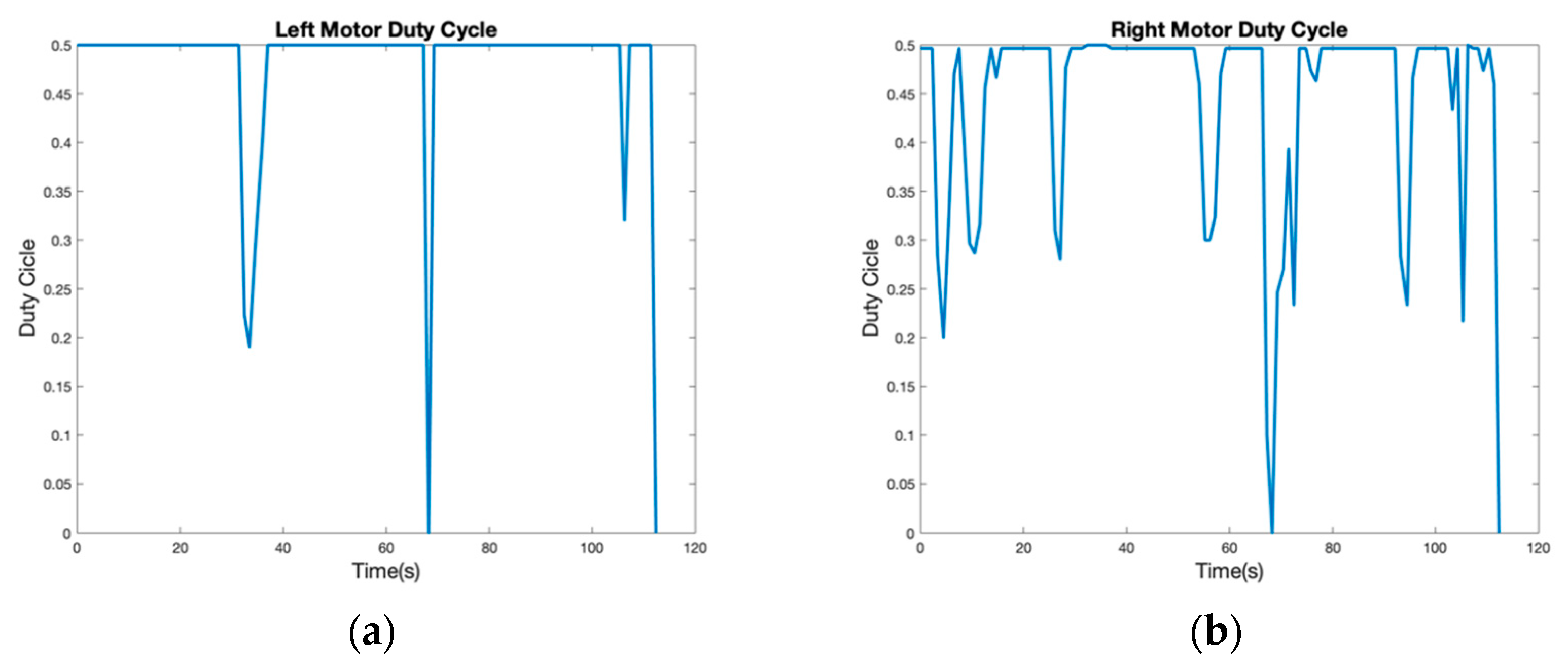
Figure 11 illustrates what happened in the trajectory. In both figures, the motor duty cycle is shown. When both duty cycles have the same value, the AMR moves in a straight line or not at all. However, when the motor control signal is reduced, the robot rotates toward the direction in which the actuator slowly moves.
Figure 11a shows that the left motor always maintains the max speed and that there are few moments featuring an obstacle on the right side. The first right side obstacle appears at 33.45 s (see the blue circle in
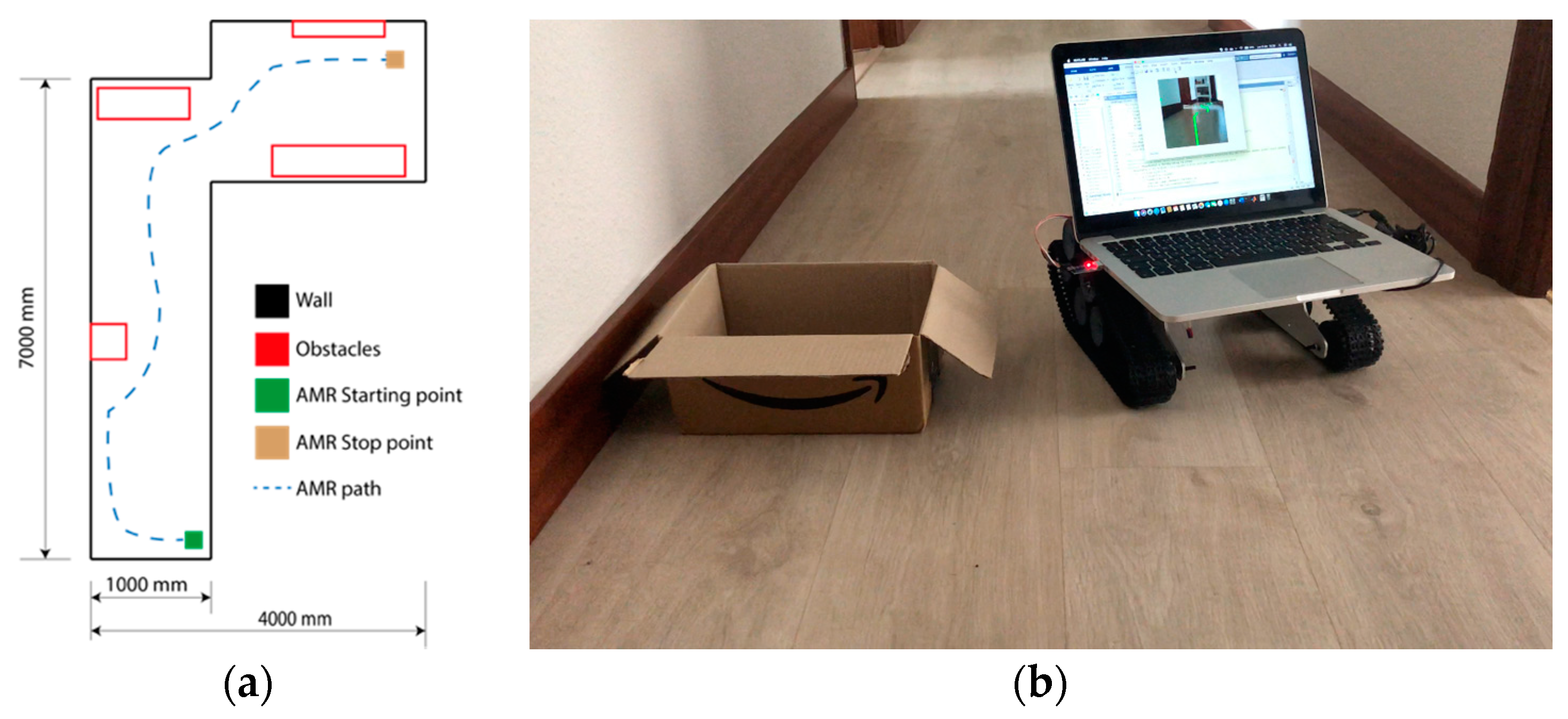
Figure 12a). For the left side motor, this reduction was about 62%, which is considerable. This reduction was probably caused by avoiding the left side obstacle, which is illustrated in a red color inside of the blue circle. The AMR has to correct each path to avoid the wall. The real scenario is represented in
Figure 12b, and the obstacle is visualized as a box.
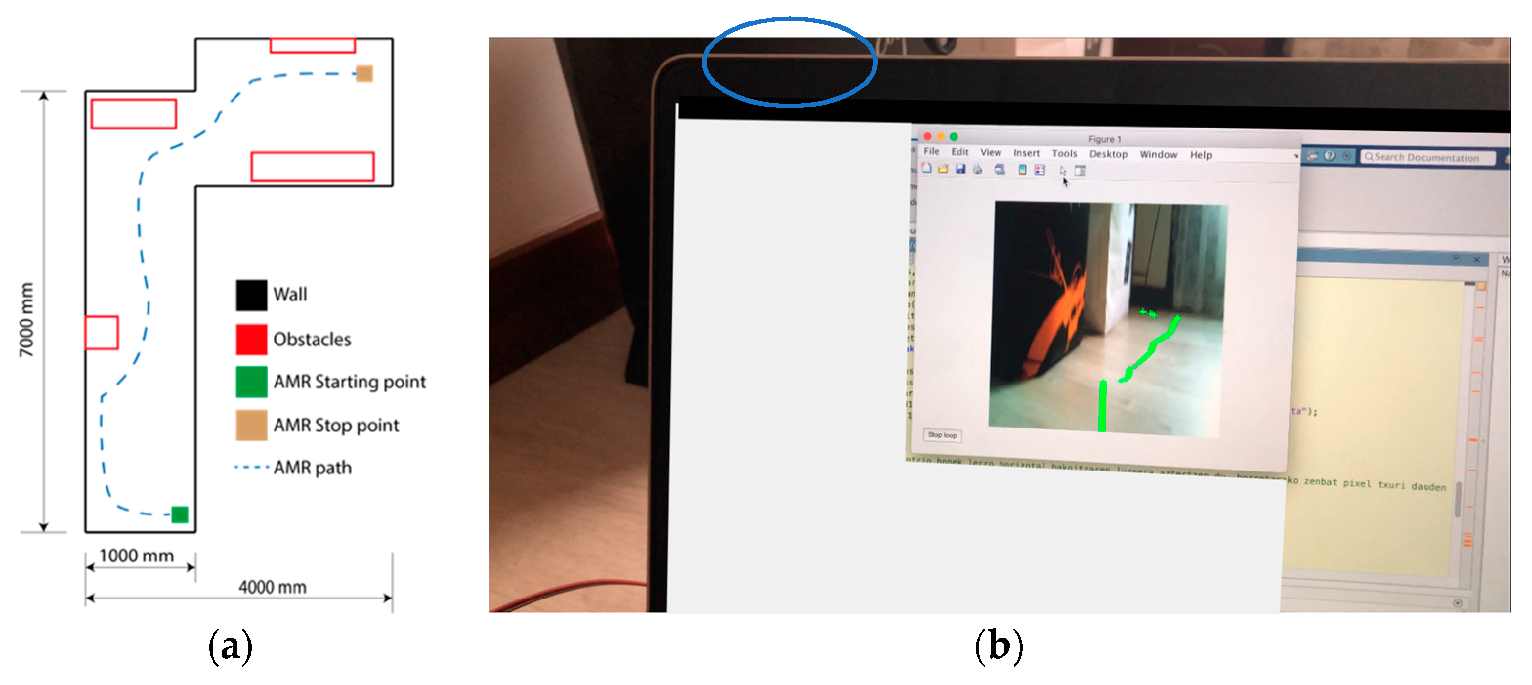
Moreover, due to its security function, the AMR stopped at 68.25 s. The mobile platform detected a nearby obstacle and decided to stop and recalculate its path.
Figure 11a,b confirms this observation. There is a null duty cycle in both situations. The blue circle in
Figure 13a determines the position and
Figure 13b shows the real situation.
The next relevant speed reduction in the left motor is observed at the bottom of
Figure 11a. There was another correction at 106.2 s, but this was an irrelevant correction used to right the path near the finish point. This correction can be defined as irrelevant because it reduced the AMR’s speed from 0.5% to 0.32%. The last speed reduction occurred at time 112.35 s, when the AMR arrived at the end position (
Figure 11). In both illustrations, the speed is the same. This end position is determined by the user, since there is a nonstop condition in the AMR.
The right motor duty cycle represented in
Figure 11b is more chaotic than that of the left side motor. The first two cycle reductions were implemented to avoid the wall, and the first reduction was made at time 4.45 s and the second at 10.5 s. the AMR starts in the wall direction (
Figure 9 and
Figure 14).
The next relevant duty reduction occurs in 27.1 s. The mobile robot has to avoid the box illustrated in
Figure 12b. In 55.2 s, the AMR avoids the obstacle represented in
Figure 13a. Before the AMR stops, it has to avoid the furniture in order to avoid a collision. Afterwards, the mobile robot stops to recalculate its path. Additionally,
Figure 15 shows that there are other obstacles in 94.6 s and 105.3 s. These obstacles include some bags situated in the path to interrupt the trajectory.
Table 2 summarizes sequences all events with a brief description.
Table 2 is divided into four sectors, and each sector is divided into time intervals with the relevant consequences.
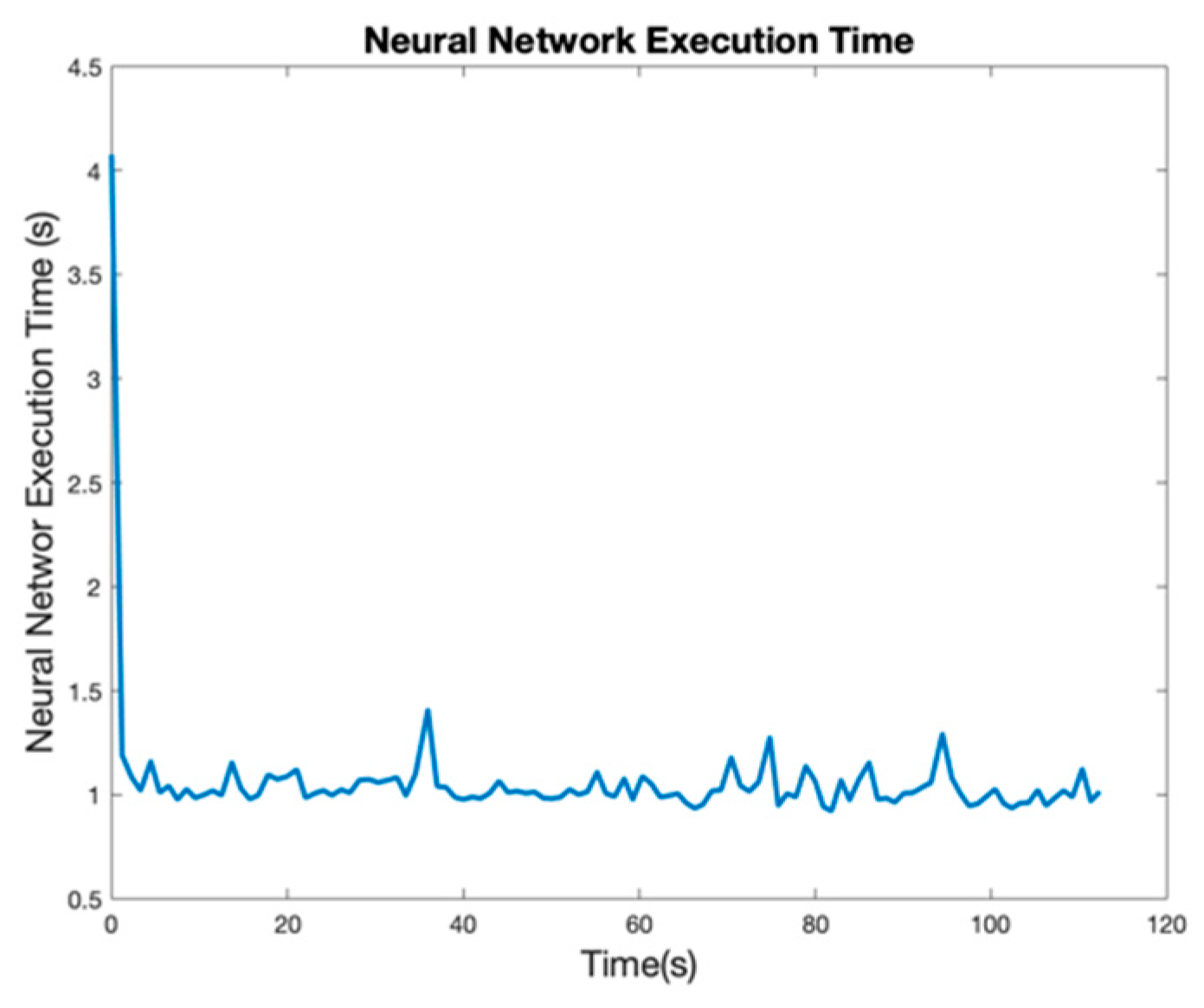
In addition to these duty cycle analyses, the neural network requires a graphics processing unit (GPU) as hardware. The execution time is reduced considerably thanks to the use of a GPU. However, our AMR uses a central processing unit (CPU) instead of a GPU. Thus, the experimental executions times are longer.
Figure 16 illustrates ResNet-18’s execution time.
The execution time reveals that the Neural Network needs 1.05 s as a median, with a maximum value of 1.408 s. Therefore, this reaction takes time in some circumstances. In case a pedestrian appears in the trajectory, the AMR needs about 1 s to react and change its direction. Moreover, the first time that the neural network is started, the CPU needs more than 4 s to start; then, the time is considerably reduced. This demonstrates that GPUs are essential for CNNs. However, the proposal of the present study is to determine if semantic segmentation works to develop an indoor navigation algorithm.
Moreover, the industrial indoor navigation system runs at 20 Hz, meaning that it runs at 0.05 s, which is clearly less that our CPU in this experiment. Thus, a small video was recorded with the AMR by moving the robot in the scenario with a joystick. The video is executed using computers to visualize the advantages of GPUs in these situations.
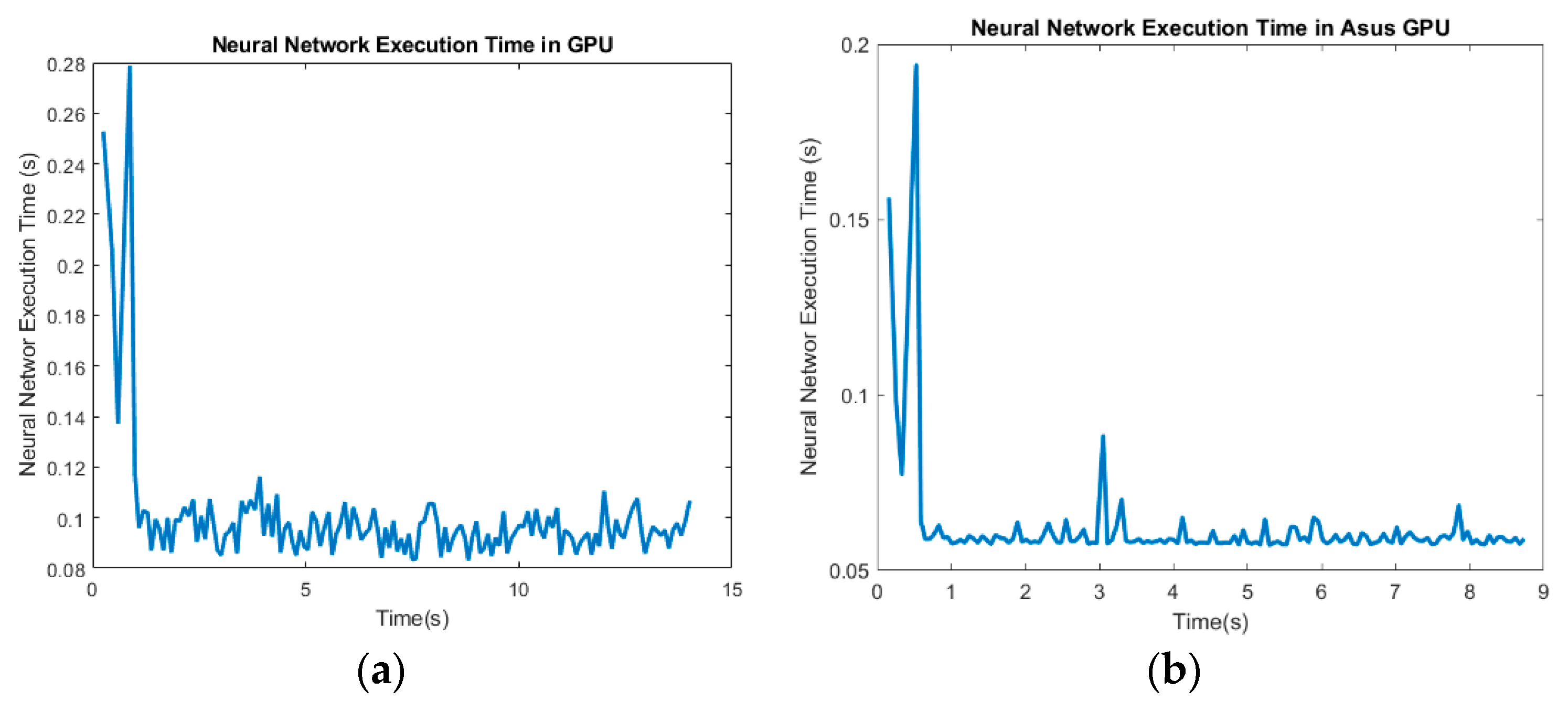
Figure 17a shows the neural network execution time on a Quadro P1000 with 640 Compute Unified Device Architecture (CUDA) cores and 4 GB DDR5 with 82 Gb/s bandwidth and on an Asus GeForce GTX 660 Ti (
Figure 17).
The results in
Figure 17a show the improvement in the speed calculation with a mean of 0.0987 s. The other GPU is an Asus GeForce GTX 660 Ti with 1344 CUDA cores and 2 GB DDR5 with 144.2 Gb/s bandwidth. Comparing the characteristics, the Asus GPU has a better CUDA cores and a higher bandwidth. However, its available memory is 2 GB less in the second computer. The results for the Asus reveal that a GPU with more CUDA cores and a memory interface, which is 128 bits in the Quadro and 192 bits in the Asus, help to compute ResNet-18 faster. The mean of this execution is 0.0615 s, which is 0.03 s faster. Therefore, this Neural Network can work with 16 Hz, which is close to the value of industrial navigation systems. Due to its CPU and other hardware components, the Asus computer also finished image processing more quickly.
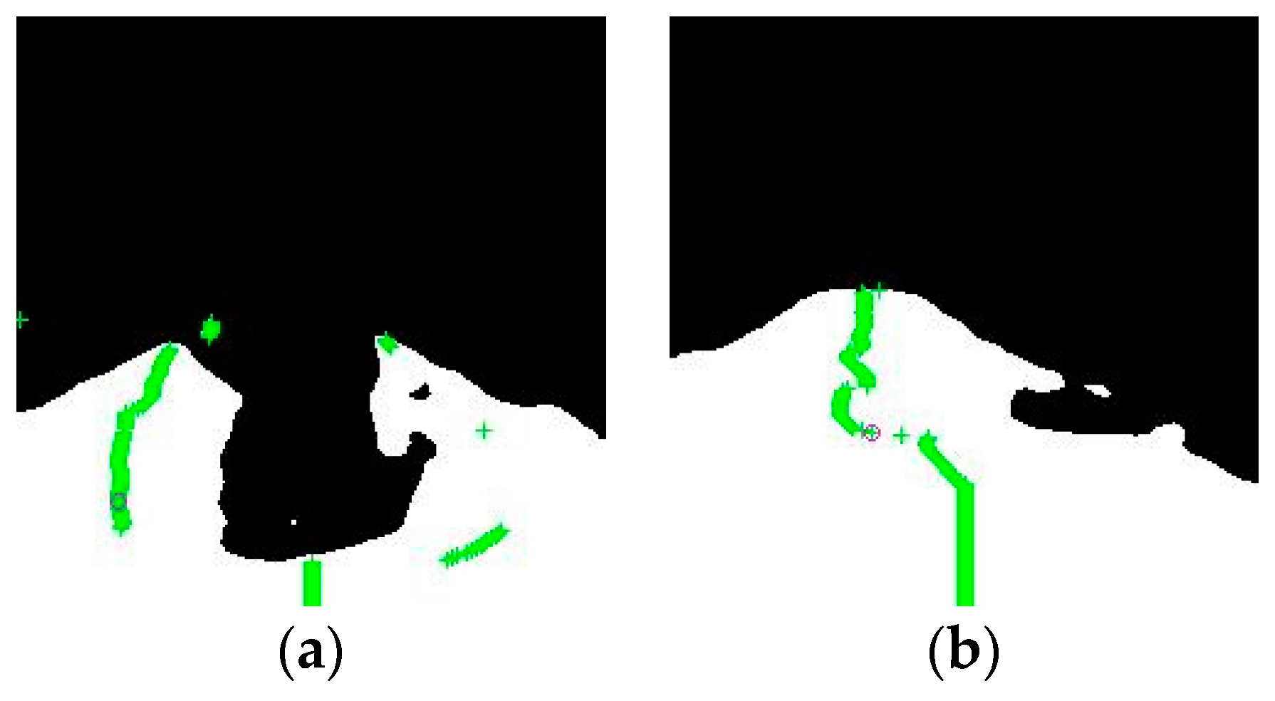
During the video recording, some obstacles were implemented in the scenario to check the path calculations.
Figure 18 illustrates some of these binary images. The floor is represented by a white color and the obstacles/walls by black.
In order to preserve the pedestrian’s identity, these images are shown as a binary. Moreover, to view which path point is selected to follow, a magenta circle is included in all the images in
Figure 18. In
Figure 18a, the pedestrian is located in the center of the corridor. Here, the path calculation has to determine the higher space and move the robot to that position. In
Figure 18b,c, the pedestrian is located on the right side of the corridor, and the AMR continuously moves to the center of the free space. Arguably, semantic segmentation works in dynamic environments when the pedestrians interrupt the AMR path. Because this neural network is executed in a CPU, the path calculation has a 1.05 s delay. Hence, this hardware is not able to safely to avoid pedestrians.
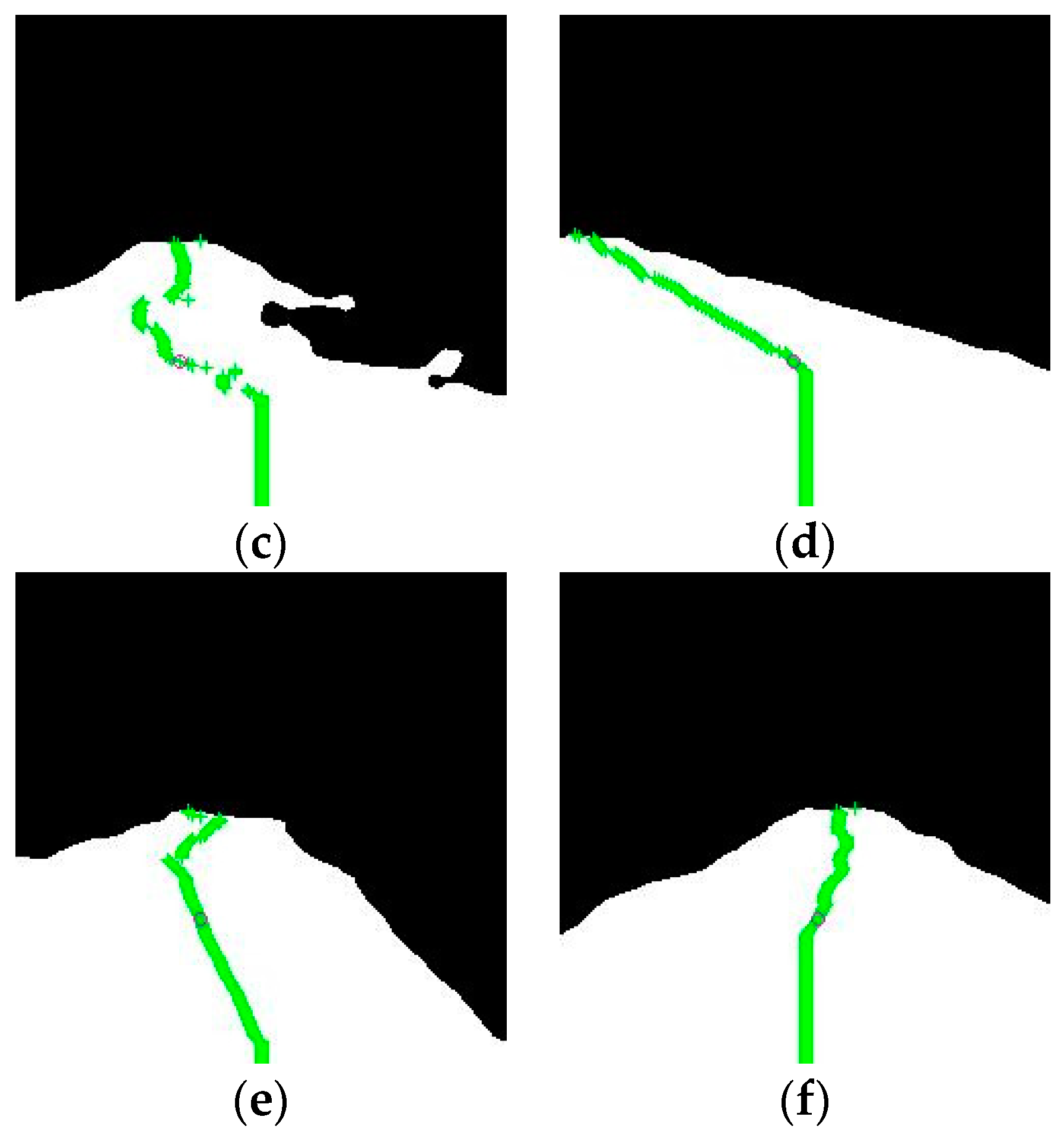
Moreover,
Figure 18d–f shows no obstacles in the corridor, demonstrating how this method makes path calculations in a free space. In
Figure 18d, the “g” parameter limitation value, which is given by Equation (16), is illustrated. In this particular instance, the AMR does not anticipate the corner by commanding a lower duty cycle for the left motor. It will wait to approximate the corner slightly more before correcting the trajectory. If the
limit changes, the AMR actuation will change. Then, the decision is to focus on what happens near the robot, rather than analyze all paths.
In order to stop the comparison, another segmentation net is created using the same training criterion and execution conditions. The aim is to represent the computational difference when the net structure becomes more complex. Therefore, ResNet-50 is modified by DepLabV3+, Vgg19 Segnet is modified with an encoderDepth of 5, and a Unet is built with an encoderDepth of 4 to segment the same scenario images. The encoderDepth values of these networks determine the number of times the input image is downsampled or upsampled. The encoder network downsamples the input image by a factor of 2D, where D is the value of the encoderDepth. The decoder network unsamples the encoder network output by a factor of 2D. Segnet(vgg19) uses the default D value, and Unet implements the 4 values similar to Segnet. These two networks have similar architectures. However, Segnet can be implemented with pretrained weights, such as vgg16 or vgg19. These networks were executed on the same laptop used in the AMR.
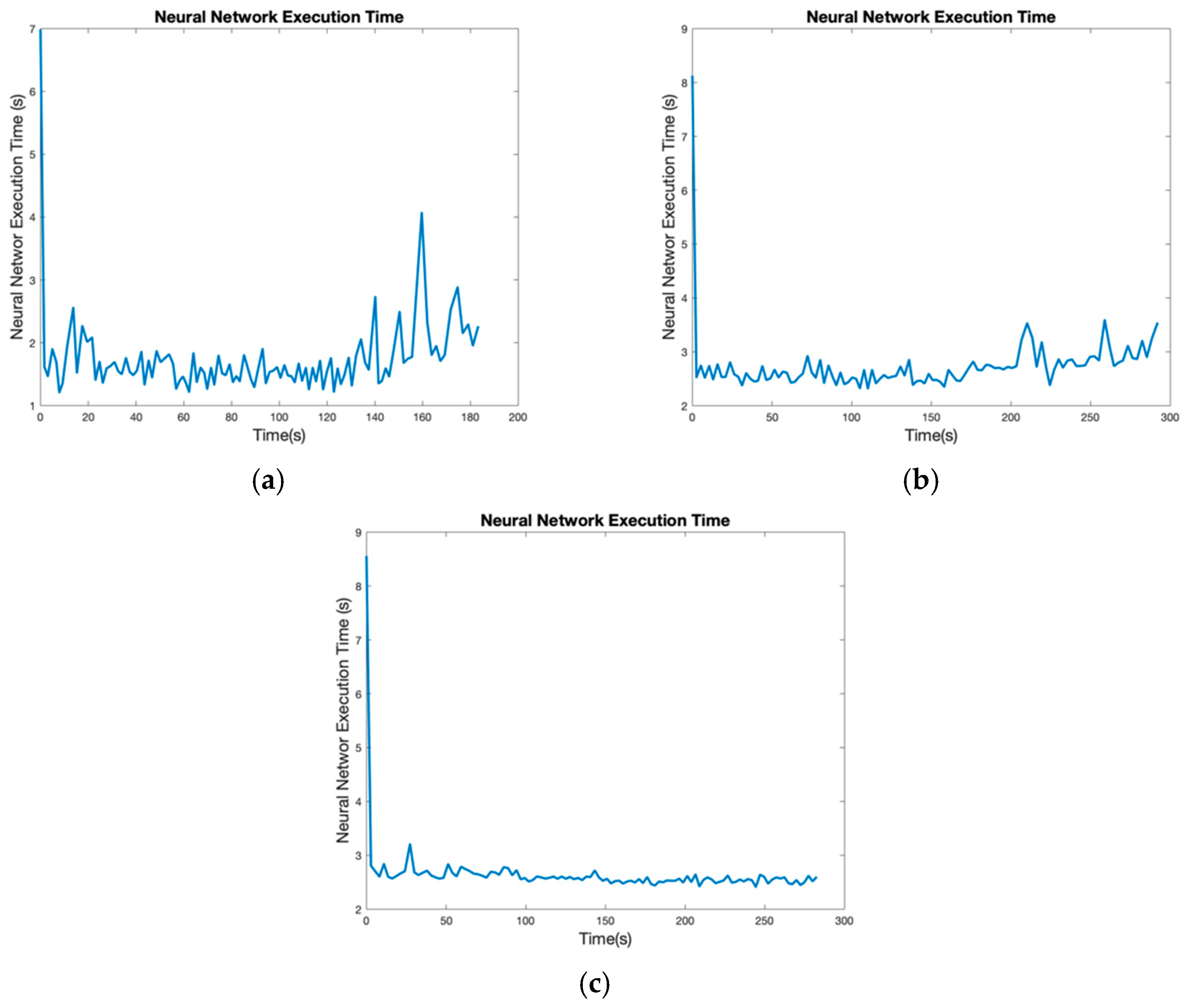
Figure 19 illustrates how more complex networks require more time to realize the segmentation calculations. The mean value of ResNet-50’s execution is 1.6739 s, and the median is 1.584 s. Comparing the results with those of
Figure 16, ResNet-50 is about 0.53 s slower. Thus, ResNet-18 is chosen because the AMR uses a CPU and is a limited type of equipment. Moreover, the CPU has to compute other programs; thus, in some cases, certain high values change. However, the GPU is a specific type of equipment used to calculate determination tasks and includes particular hardware to compute tasks simultaneously. The Segnet(vgg19) and Unet execution mean values are 2.84 s and 2.56 s, respectively. This confirms that Resnet-18 is a good choice for limited hardware contexts.
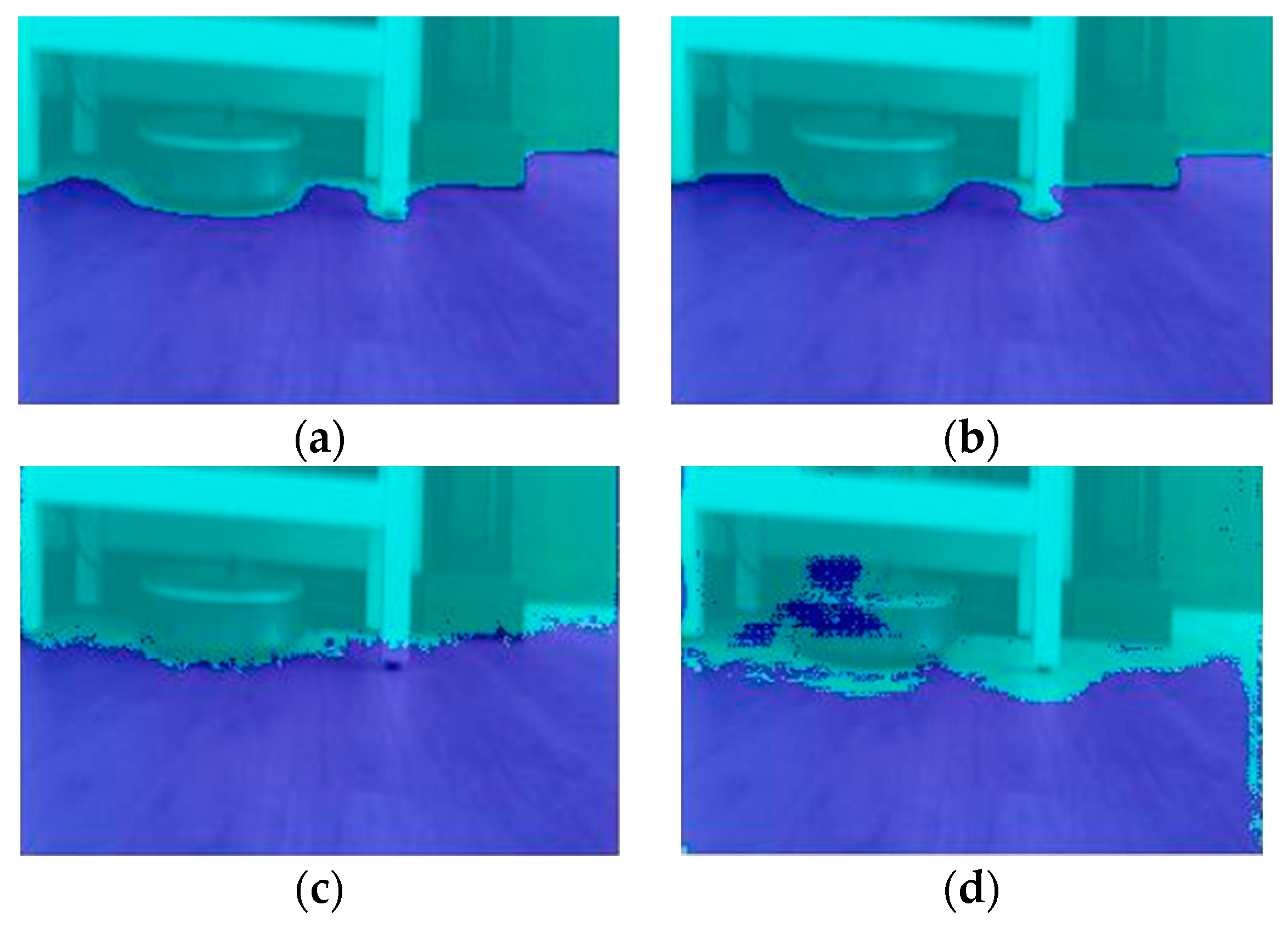
The semantic segmentation network accuracy values are represented in
Table 3, and the scene segmentation results are visualized in
Figure 20. The results reveal that ResNet is overfitted to this scenario and has difficulties adapting to other scenarios. However, for industrial applications, it seems logical to train a net that works in particular surroundings because the indoor environment does not change as quickly as the outdoors. In other words, outdoor mobile platforms have to adapt constantly (e.g., light conditions due to the weather changing the luminance, road line degradation, etc.).
However, Segnet(vgg19) and Unet have greater difficulty segmenting the scenario properly. Resnet has a better resolution, as indicated by its speed and accuracy results. This performance is fixed to the data set preparation and training options. Hence, in future work, other architectures, data sets, training options, etc. will be tested to improve the performance of this navigation technique. Nevertheless, the present work reveals how to use the resulting mask of the net to develop a navigation technique.
4. Conclusions
The main goal of the present study was to develop an indoor navigation for an AMR by implementing a CNN that segments the image to determine a navigable zone and calculate the steering and speed commands by applying different mathematical operations.
ResNet-18 can segment the image, and the proposed mathematical equations can use this information to provide a path for the AMR. Nevertheless, the Neural Network execution time in the CPU is not sufficient to provide safety features in sudden situations. The mean value of each result was about 1.05 s, which is insufficient for industrial autonomous mobile robots. The industrial applications work with a 10 Hz frequency. Therefore, the Neural Network with a CPU is not useful for navigation. In this case, to provide safe navigation, the speed of the AMR has to be reduced. However, by executing ResNet-18 in the GPU, the situation changes. The results reveal that the conventional Nvidia GPU runs the net around 16 Hz.
With this CPU configuration, the mobile robot using the present sematic segmentation can avoid different obstacles. It can differentiate between the floor and the rest of the obstacles and calculate new following points by determining the free space conditions. The subsequent point is between two limits, and the worst-case scenario is always assumed, which is evaluated by measuring the difference between the horizontal line middle point estimation and the center of the image. If the worst case is located on the right size, the AMR follows it by adapting the motor duty cycle.
In future work, an AMR will be equipped with a Nvidia Jetson AGX that has 512 CUDA cores with 32 GB 256-Bit LPDDR4x and 137 GB/s bandwidth. These specifications are better than those of Asus or Quadro due to its higher computational capacity thanks to its memory. Moreover, the training and the path following algorithms will be improved by adopting new scenarios and mathematical equations, such as a path planning algorithm, which can intelligently move the AMR to a specific location. To improve the AMR’s adaptability to other indoor scenarios, other types of net will be tested. These networks will be implemented on a Nvidia Jetson AGX to improve the application time response. An automatic labeler will also be developed.

 ,
, 


