A Power Maxwell Distribution with Heavy Tails and Applications


1
Departamento de Matemáticas, Facultad de Ingeniería, Universidad de Atacama, Copiapó 1530000, Chile
2
Departamento de Ciencias Matemáticas y Físicas, Facultad de Ingeniería, Universidad Católica de Temuco, Temuco 4780000, Chile
3
Departamento de Matemática, Facultad de Ciencias Básicas, Universidad de Antofagasta, Antofagasta 1240000, Chile
*
Author to whom correspondence should be addressed.
Mathematics 2020, 8(7), 1116; https://doi.org/10.3390/math8071116
Submission received: 28 May 2020
/
Revised: 26 June 2020
/
Accepted: 28 June 2020
/
Published: 7 July 2020
(This article belongs to the Section Probability and Statistics)
Abstract
:In this paper we introduce a distribution which is an extension of the power Maxwell distribution. This new distribution is constructed based on the quotient of two independent random variables, the distributions of which are the power Maxwell distribution and a function of the uniform distribution (0,1) respectively. Thus the result is a distribution with greater kurtosis than the power Maxwell. We study the general density of this distribution, and some properties, moments, asymmetry and kurtosis coefficients. Maximum likelihood and moments estimators are studied. We also develop the expectation–maximization algorithm to make a simulation study and present two applications to real data.
1. Introduction
A distribution related to the normal distribution is the slash distribution. Its stochastic representation is the quotient between two independent random variables: a normal distribution and a function of the uniform distribution. Thus we say that S has a slash distribution if:
where , Z is independent of U and . When we obtain the slash canonical distribution, and when we obtain the standard normal distribution. The density of the canonical slash is:
where represents the standard normal density defined in Appendix A (see Johnson et al. [1]). This distribution has much heavier tails than the normal distribution; i.e., it has greater kurtosis. Some properties of this family are discussed by Rogers et al. [2] and Mosteller et al. [3]. The maximum likelihood (ML) estimators of scale and location are discussed in Kafadar [4]. One paper Wang et al. [5] introduced a multivariate version of the slash distribution and a skew multivariate version. Reference Gómez et al. [6] extended the slash distribution using the family of univariate and multivariate elliptical distribution. Reference Gómez et al. [7] used this family to extend the Birnbaum–Saunders distribution. Reference Iriarte et al. [8] and Gómez et al. [9] used this methodology to extend the generalized Rayleigh distribution and Gumbel respectively. Reference Olmos et al. [10] also used this methodology to introduce the modified slashed half-normal distribution. Reference Olmos et al. [11] recently introduced the confluent, hypergeometric slashed-Rayleigh distribution using the same methodology.
The Maxwell distribution was first set out by Maxwell [12], and gave the distribution of velocities among the molecules of a gas. Maxwell’s finding was generalized by Boltzmann [13,14,15], to express the distribution of energies among molecules. It has several statistical applications in the areas of physics, chemistry, and physical chemistry, (see Dunbar [16]). For example, in the context of the kinetic molecular theory of gases, a gas contains a large number of particles in rapid motion. Each particle has a different velocity, and each collision between particles changes the velocities of the particles. An understanding of the properties of the gas requires an understanding of the distribution of particle velocities (which is the Maxwell distribution). In addition to these areas, it also has uses in the theory of relativity. Ideal plasmas, which are ionized gases of sufficiently low density, frequently have particle distributions that follow the Maxwell distribution.
Coraddu et al. [17] discussed the physics of nuclear reactions in stellar plasma by checking with special emphasis on the importance of the velocity distribution of ions. Then they claimed that the properties (density and temperature) of the weak-coupled solar plasma were analyzed, showing that the ion velocities should deviate from the Maxwell distribution and could be better described by a "weakly-non-extensive Tsallis" distribution.
Singh et al. [18] introduced the power Maxwell (PM) distribution; i.e., we say that X has a PM distribution if its density function is:
where is a scale parameter and is a shape parameter. We denote it as , where:
The main object of this paper is to introduce an extension of the PM distribution using slash methodology. This new distribution presents a greater kurtosis than the PM distribution, so we can use it to model atypical data. In Section 2, we introduce the slash power Maxwell (SPM) distribution, with its stochastic representation, its distribution and its survival and hazard functions. Then we focus on the moments of the distribution, asymmetry and kurtosis coefficients. We devote Section 3 to the study of some properties of the model, such as the mode, the convergence, and the distribution of the stochastic order. We assign Section 4 to inference, wherein we obtain the moments and ML estimators, and establishing the expectation–maximization (EM) algorithm. In Section 5 we present the simulation study, focusing our attention on parameter recovery and criteria comparison. In Section 6, we present two applications to real data, fitting the PM distribution to the datasets; and finally, in Section 7 we present our conclusions.
2. Probability Density Function
2.1. Stochastic Representation
We consider that the random variable Z has a SPM distribution with parameters , and q if it can be represented as
where and are independent, and . We denote this by writing , where q is the kurtosis parameter.
2.2. Density Function
The following proposition presents the probability density function (pdf) distribution that can be generated using (3).
Proposition 1.
Let . Then, the pdf of Z is given by
where is the scale parameter, is the shape parameter, is the kurtosis parameter, is the gamma function defined in Appendix A and is the cumulative distribution function (CDF) of the gamma distribution also defined in Appendix A.
Proof.
Using the representation given in (3) and computing the Jacobian transformation, we have that
Then, , so that by marginalizing with respect to the random variable W, we obtain the density function corresponding to the random variable Z; namely:
so making the variable change , the result is obtained.□
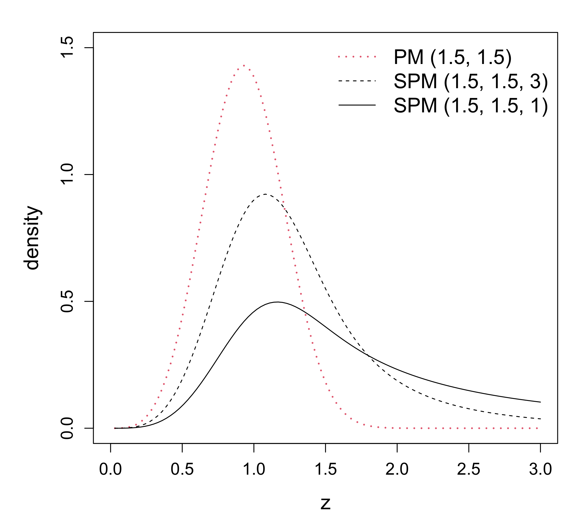
Figure 1 shows the density of SPM for some values of parameter q. It reveals that the tails become heavier as q becomes smaller.
In Table 1 we perform a brief comparison, illustrating that the tails of the SPM distribution are heavier than those of the PM distribution, showing for different values of z in the distributions mentioned. It is clear that the SPM distribution may have much heavier tails than the PM distribution.
Proposition 2.
Let . Then the CDF of Z is given by:
Proof.
By integrating by parts the kernel of the density
using and we finally obtain
and then, by substituting in the last integral (i.e., ), we obtain
Thus the proof is complete.□
Corollary 1.
Let . Then the survival function and the hazard function of Z are given
where and .
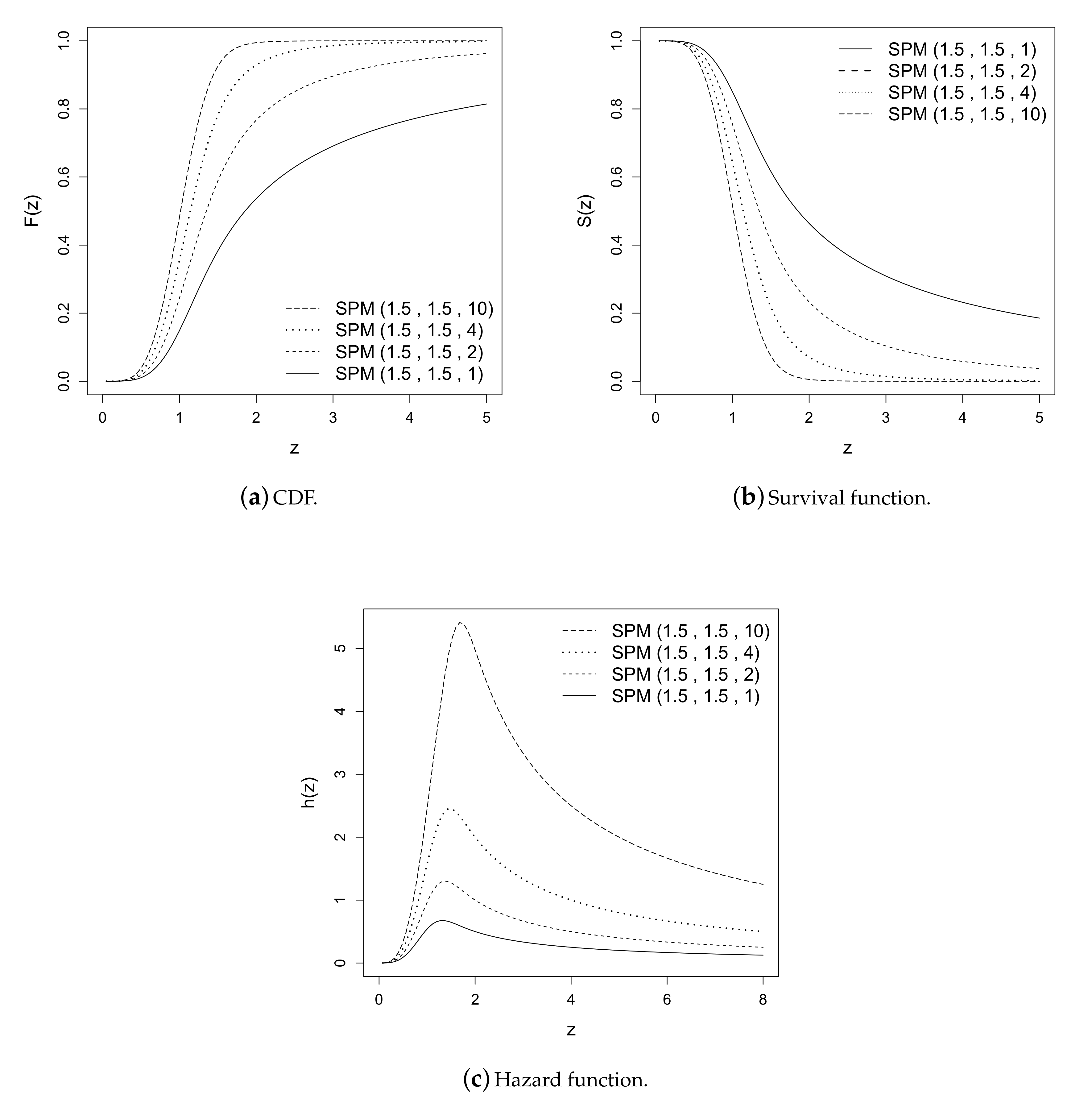
In Figure 2, we show the CDF, survival and hazard functions. Additionally, we can see that the curve related to the hazard function is unimodal, and that as "q" grows, the curve has longer tails and extends to a greater range.
Proposition 3.
Let . Then the mode of Z can be obtained by solving:
where and . This equation must be solved numerically.
Proof.
We set , we have
Considering
the result is obtained.□
2.3. Distribution Relationships
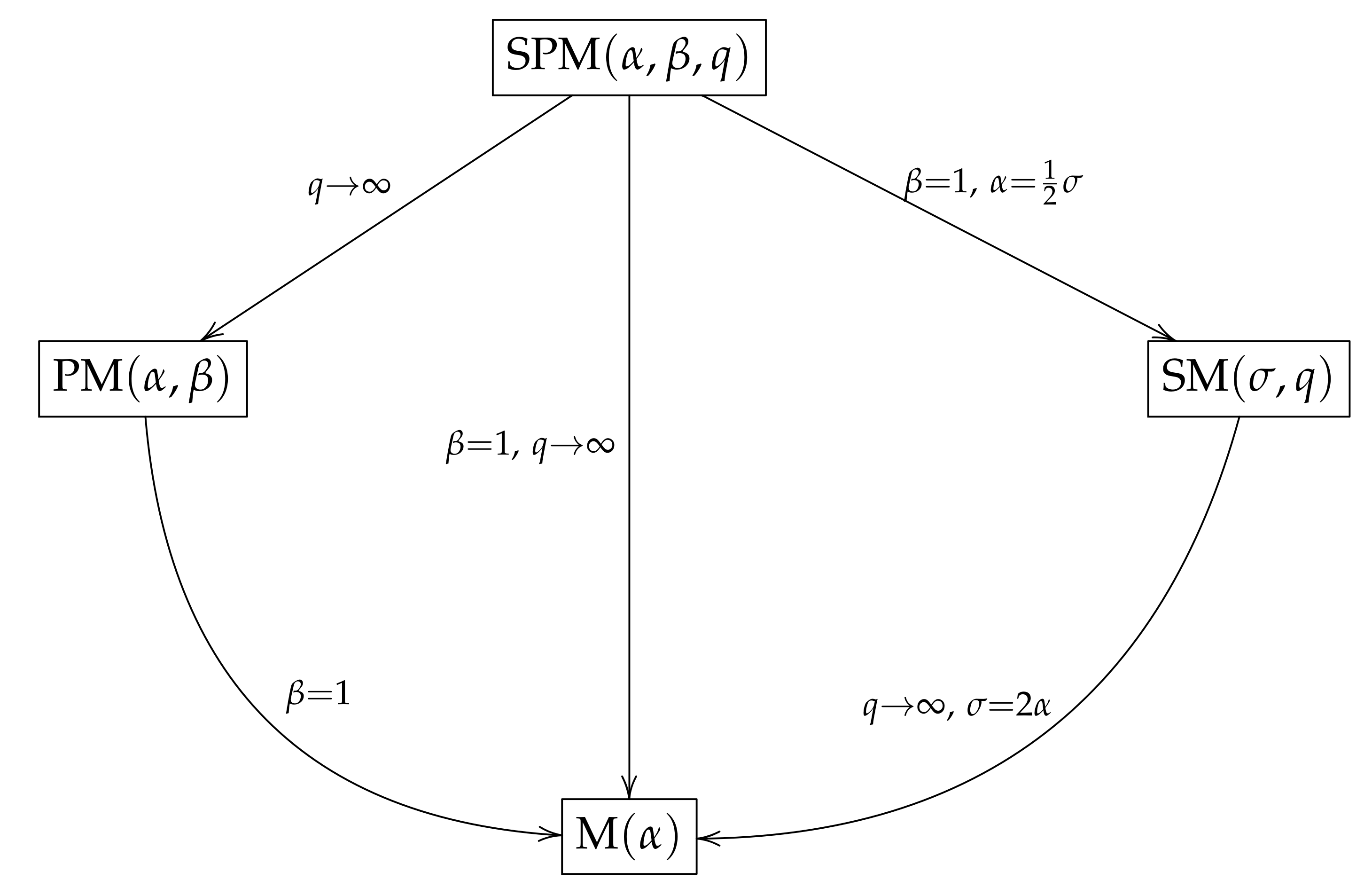
It is easy to see some special cases that are associated with SPM distribution.
- According to a property that we will discuss later in Section 3, if then , where ).
- If then with , where Y has slash Maxwell (SM) distribution (Iriarte et al. [8]).
- If and , then , where M has Maxwell distribution.
A diagram showing this relationship is presented in Figure 3.
2.4. Moments
We present a general formula for the rth moment of the SPM distribution.
Proposition 4.
Let Then, for , it follows that the rth moment of Z can be written as
Proof.
Using the stochastic representation for the distribution given in (3), we have that
where , and are the moments of the .□
Corollary 2.
If , then it follows that
where are the r-moments of the PM distribution.
Remark 1.
The asymmetry and kurtosis coefficients can be obtained using:
Corollary 3.
Let ; then the asymmetry coefficient and the kurtosis coefficient for and respectively
where , and is the rth moment of the distribution.
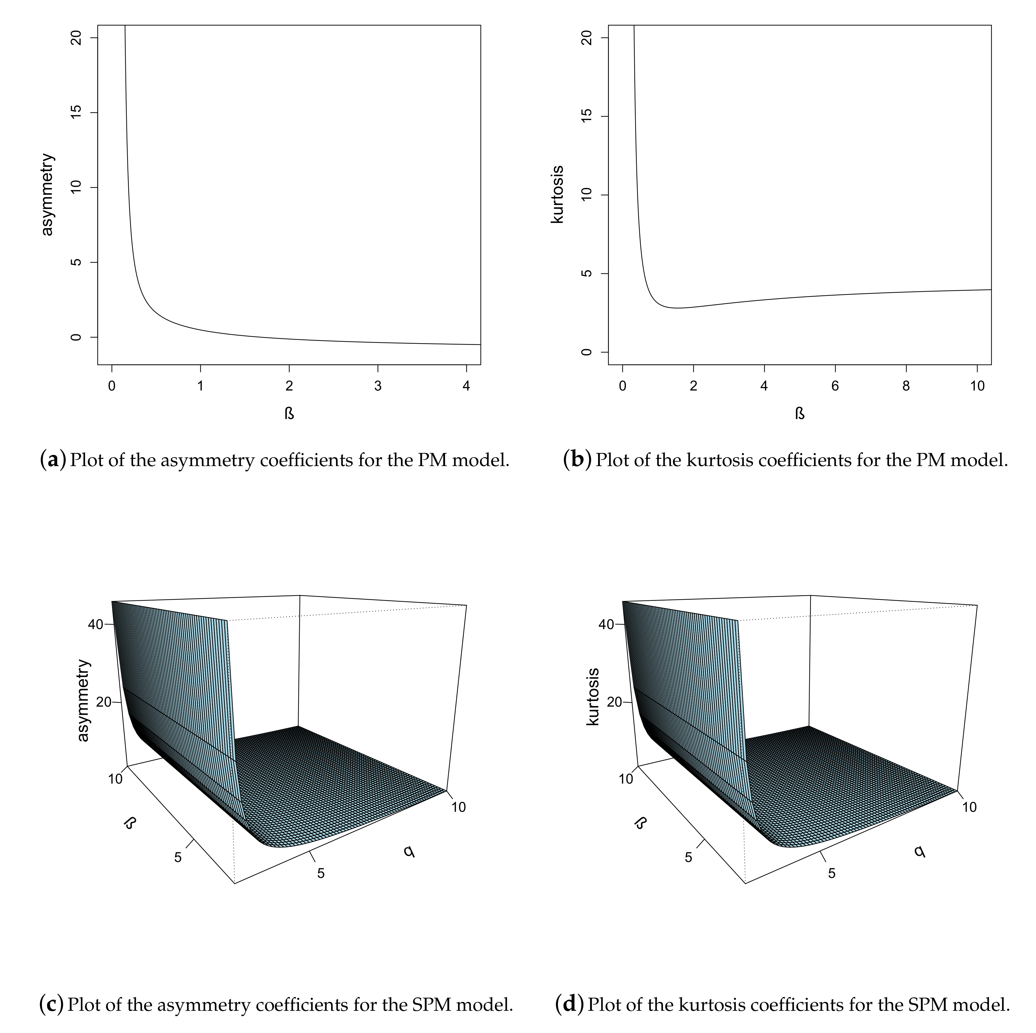
Figure 4a,b show in graphic form the asymmetry and kurtosis coefficients of the PM model for different parameter values. Figure 4c,d show the asymmetry and kurtosis coefficients of the SPM model for different parameter values. It can be seen that both coefficients increase when the parameter q decreases. When observing the Figures for both models, it is evident that the SPM distribution covers a wide range of values for the asymmetry and kurtosis coefficients, depending on the parameter values, implying that the SPM model is sufficiently flexible to model real datasets. Table 2 reveals that values for the asymmetry and kurtosis coefficients depend on the parameters and q, and that as q decreases and increases, the asymmetry and kurtosis coefficients also increase. On the other hand, as q increases the asymmetry and kurtosis coefficients are those of the PM distribution.
On the other hand, we also have that
are the asymmetry and kurtosis coefficients of the PM distribution, where .
3. Properties
This section is devoted to studying some properties of the model.
Proposition 5.
Let and ; then Z converges in distribution to X, as .
Proof.
The proof will use Lehman’s and Slutsky’s theorem (Lehmann [19], p. 70). It is easy to see that , and . Thus, if we define the function , then:
as . Thus, as .□
Proposition 6.
Let denote the order statistics of a random sample from . Then the pdf of , , is:
where and .
Proof.
Let be the order statistics of a random sample, from a continuous population with CDF and pdf . Then, the of is
Now, replace and with the pdf and CDF of the SPM distribution respectively; then the result is obtained.□
Corollary 4.
Let denote the order statistics of a random sample from . Then the pdfs of the minimum and the maximum are respectively:
where and .
Proposition 7.
Let , and . with CDF and respectively. Then is stochastically greater than .
Proof.
Recall that is stochastically greater than , if for every t, which implies . Now, notice that the second term of the distribution function of Z is always greater than or equal to zero. Then we have:
which means that .□
Table 3 shows the quantities of the mean, variance, median and mode when , and q are increasing.
We note that the quantities decrease as long as q increases.
4. Inference
This section is devoted to inference aspects for the SPM model. Parameters are estimated based on the moments and ML methods.
4.1. Moments Estimation
Replacing by the sample mean , gives the equation:
by which we obtain the moment estimator of q:
Therefore, using (5) and replacing and with the second and third sampling moments, we obtain the following equations:
where is the r-th moment of the PM distribution.
4.2. ML Estimation
In this section, we present the ML equations for parameters of the SPM model. If is a random sample from the random variable , the log-likelihood function can be expressed as
where and .
The ML estimators are obtained by maximizing the log-likelihood function given in (8). By deriving the log-likelihood function with respect to each parameter, the following estimating equations are obtained:
where , , and are the digamma function.
These equation systems need to be solved numerically using an adequate root finder procedure. The moments estimator could be used to find initial values for the iterative procedure.
The EM algorithm (Dempster et al. [20]) defines an iterative process that allows the likelihood function of a parametric model to be maximized in cases in which some variables of the model are (or in our case, are treated as) "latent" or unknown. The advantage is simple: the EM algorithm is significantly less computationally intensive and far more robust. However, we will use the expectation/conditional maximization (ECM) algorithm (Meng and Rubin [21]), which is an extension of the EM algorithm.
4.3. EM Algorithm
Using the stochastic representation (3), but considering the following parametrization , we obtain:
so we have the following hierarchical model
where is the latent variable, and is the observable variable, for . Now, consider the new parameter vector. In this case the complete-data log-likelihood or full log-likelihood function is
where is the full log-likelihood function. Then :
where and . Normally, the next thing to do is find the distribution of
but instead, we will use the distribution of :
Thus, we conclude that W follows a truncated gamma in the interval (0, 1) (shown in the Appendix A), that is, . Then:
which correspond to and respectively. The equations result from deriving with respect to the parameters:
The equation corresponding to must be solved numerically. Finally, we obtain the following EM algorithm.
Step E: calculate and using (10).
Step M: update using (11).
Once some stop criteria have been completed, calculate to obtain the estimators of . For example, one stop criteria could be .
5. Simulation
In this section we present the simulation study, which aims to investigate the ML estimation performance for parameters , , q under the SPM model; then we focus on comparison, using the AIC (Akaike [22]), BIC (Schwarz [23]), ADR and AD2R (Anderson et al. [24]) criteria. First, we present the algorithm that was used to generate samples for .
- Generate (chi squared with 3 degrees of freedom), .
- Compute , .
- Generate , .
- Compute , ,
where and are the chi-squared distribution with three degrees of freedom and the standard uniform distribution respectively.
The algorithm that was used to calculate the ADR and AD2R values is described below:
where is the CDF, and the i-th statistic of order. To calculate AIC and BIC values:
where k is the number of parameters, n the sample size and the value of the log-likelihood function using the ML estimator of .
5.1. Parameter Recovery
Using the algorithm, we generate 1000 random samples of sizes , and under the SPM model, with different parameter values. In Table 4 we present a summary of the study results. For each sample, an ML estimator was computed numerically using the EM algorithm, where the means and the standard deviations are reported. As expected, as the sample size increases, its standard deviation decreases and therefore the parameter estimate approaches the true simulated value. We conclude that the ML estimates are quite stable.
5.2. Criteria Comparison
We generated 1000 random samples of sizes , and under the SPM model using different parameter values. The following tables show the proportions of times that the respective criteria (detailed in the previous section) chose the SPM over the PM model. Table 5 corresponds to data simulated by the SPM model. Results show that when the data are drawn from the SPM distribution, the four criteria corresponding to the SPM model are usually lower than the criteria for the PM model. We also conclude that for models with heavy tails, ADR and AD2R are better criteria for evaluating model fitness.
6. Applications
We now present two applications to real datasets showing descriptive analysis and ML estimators for the M, PM and SPM models with their AIC, BIC, ADR and AD2R criteria, histograms and Q-Q plots.
6.1. Application 1
We consider a dataset of fund-raising expenses as a percentage of total expenditure for a random sample of 60 charities from the United States. These observations can be found in Devore [25], p. 4. These are:
6.1,12.6,34.7,1.6,18.8,2.2,3.0,2.2,5.6,3.8,2.2,3.1,1.3,1.1,14.1,4.0,21.0,6.1,1.3,20.4
7.5,3.9,10.1,8.1,19.5,5.2,12.0,15.8,10.4,5.2,6.4,10.8,83.1,3.6,6.2,6.3,16.3,12.7,1.3,
0.8,8.8,5.1,3.7,26.3,6.0,48.0,8.2,11.7,7.2,3.9,15.3,16.6,8.8,12.0,4.7,14.7,6.4,17.0,
2.5,16.2
In Table 6, we can see from the descriptive analysis that this dataset has high kurtosis.
Table 7 shows the ML estimates for the parameters of the M, PM and SPM distributions. For each model, we apply the statistical criteria named at the beginning of this section; we see that all four criteria choose the SPM model over the M and PM models.
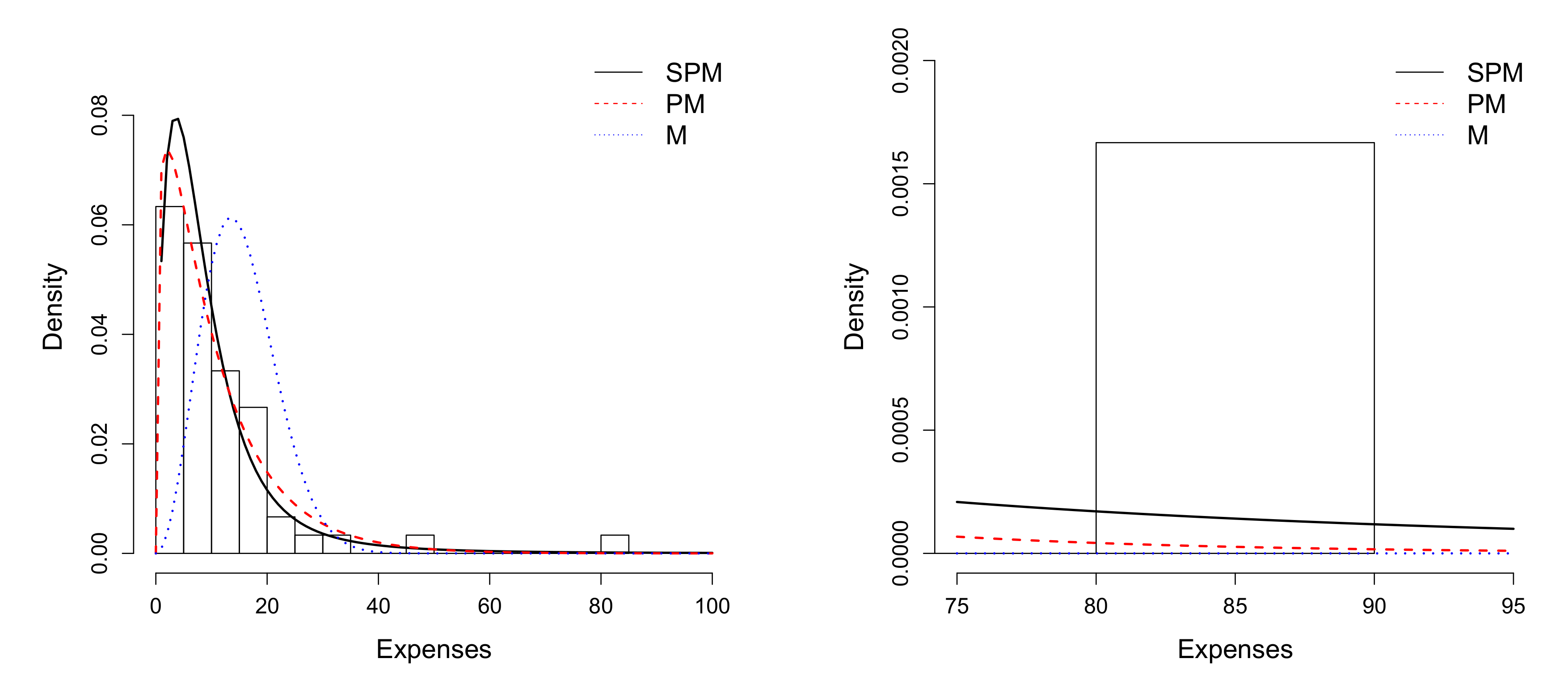
Figure 5 depicts the histogram of the dataset, where we can check that the SPM model has a greater reach than the other models.
6.2. Application 2
We consider a dataset of the copper content of 24 Bidri products (a traditional Indian handicraft); this study was performed because Bidri crafts are soldered with an alloy containing mainly zinc and some copper (Devore [25], page 33). These are:
2.0, 2.4, 2.5, 2.6, 2.6, 2.7, 2.7, 2.8, 3.0, 3.1, 3.2, 3.3, 3.3, 3.4, 3.6, 3.6, 3.6,
3.7, 4.4, 4.6, 4.7, 4.8, 5.3, 10.1
In Table 8, we can see from the descriptive analysis that this dataset has high kurtosis, so it is interesting to see what our model can do here.
Table 9 shows the ML estimates for the parameters of the M, PM, and SPM distributions. For each model we apply the statistics criteria named at the beginning of this section, and we see that all four criteria choose the SPM model over the M and PM models.
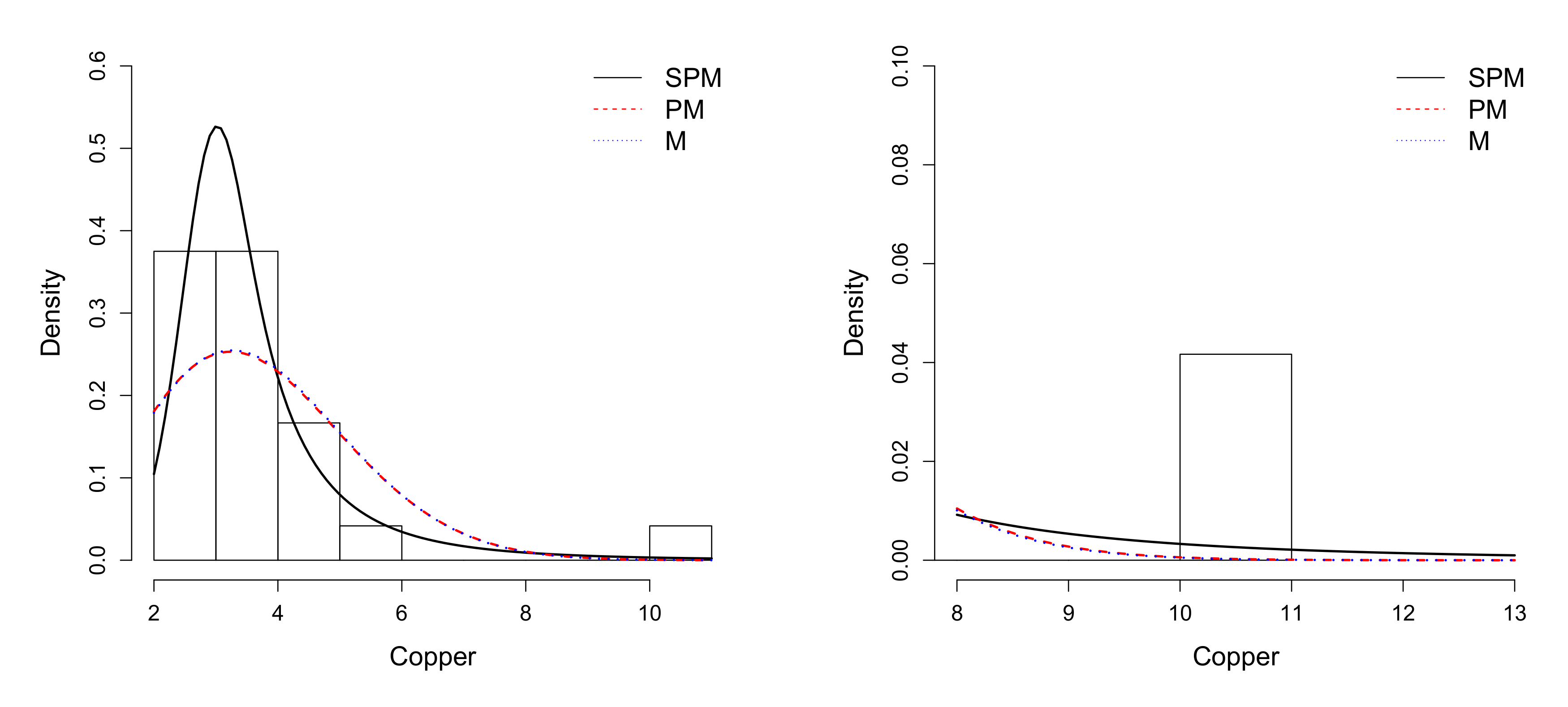
Figure 7 depicts the histogram of the dataset, where we can check that the SPM model has a greater reach than the other models.
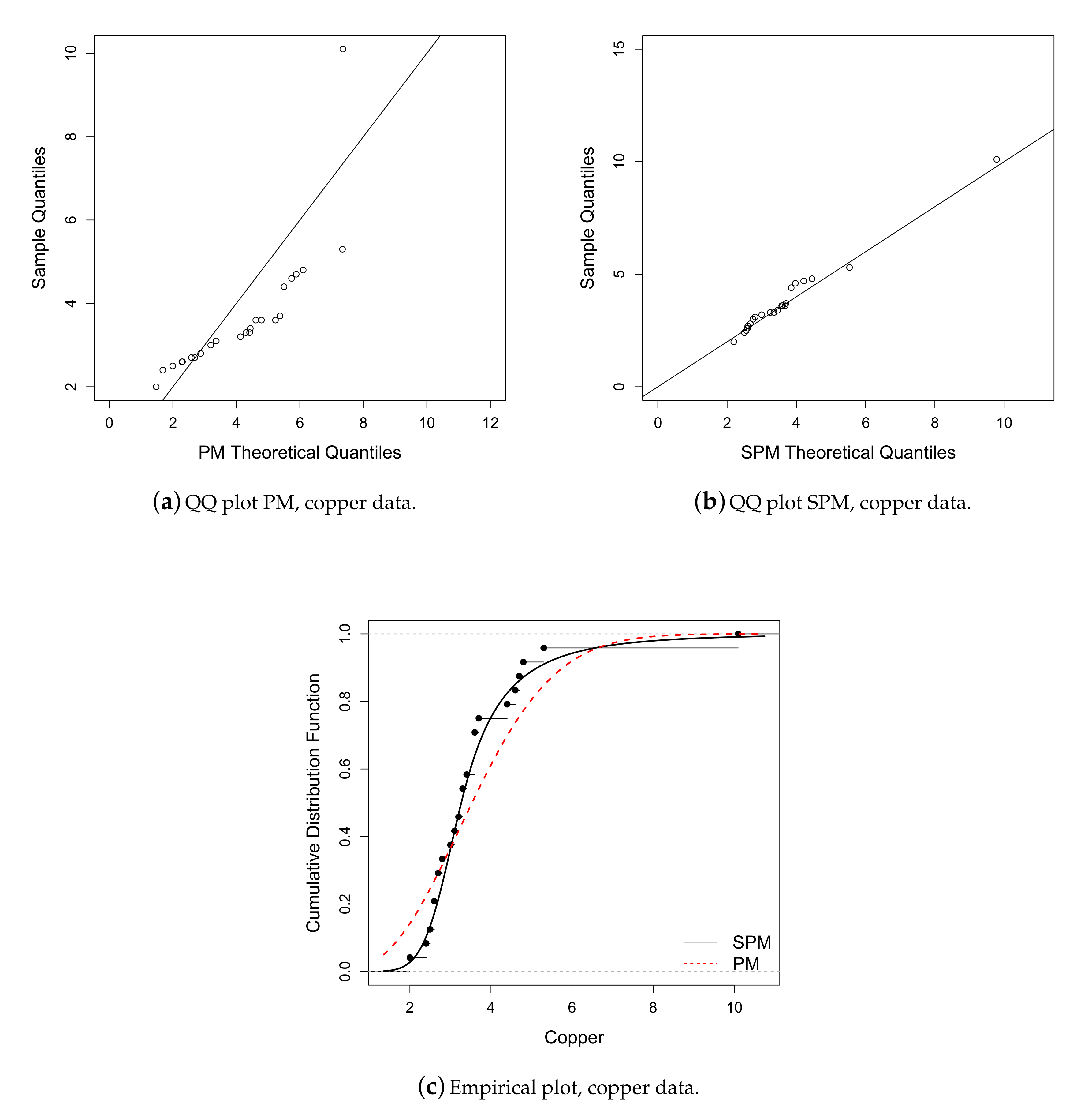
Finally, Figure 8a,b show the Q-Q plots for the PM and SPM models respectively, and Figure 8c shows the empirical plot, which tells us that the SPM model is preferable.
It is interesting to note that the estimate of the shape parameter of the PM model is almost 1; remember that if , then we obtain the classic M distribution.
7. Conclusions
The slash methodology has often been used recently to extend a variety of well-known distributions, resulting in a flexible distribution that has high kurtosis, and of course heavier tails, as we discuss above. Here we introduced the SPM distribution, where following the same methodology, we extended the PM distribution by using the PM instead of the normal model; see Equation (1). So the PM is a special case of the SPM model. As we saw in Figure 1, the new distribution does indeed present a more flexible kurtosis coefficient than that of the PM model; moreover, as we saw in Table 1, the tails become heavier as parameter q becomes smaller.
We discussed some properties, such as the distribution, survival and hazard functions. We also studied the mode; moments; statistic order; and of course, asymmetry and kurtosis. They all have closed form, which makes computational implementation easier. We also presented two stochastic representations: One is defined as a quotient between two independent random variables: PM in the numerator and the power of a standard uniform distribution in the denominator. The second is a mixture of a PM and a beta distribution, used to establish the EM algorithm.
Parameters could be estimated using the moments method and ML estimators using log-likelihood or EM algorithm methodology, although the EM algorithm is more stable, as we obtained closed expressions.
The results of a simulation study were presented, indicating good parameter recovery. In the simulation study for the criteria, we concluded that the criterion which best explained the fit of the SPM model was AD2R.
In the application we used datasets with high kurtosis, which seems logical considering the object of the work. Four model comparison criteria statistics were used; all four criteria indicate that the SPM model shows the best fit for this dataset. The ADR and AD2R criteria are more reliable for comparing distributions using two real datasets; this can be seen in the application, where these criteria showed a better fit for the SPM model.
Author Contributions
Conceptualization, F.A.S. and Y.M.G.; Formal analysis, F.A.S., Y.M.G., O.V. and H.W.G.; Investigation, F.A.S, O.V. and H.W.G.; Methodology, Y.M.G. and H.W.G.; Software, F.A.S; Supervision, Y.M.G.; Validation, H.W.G.; Writing original draft, H.W.G.; Writing review and editing, O.V. All of the authors contributed significantly to this research article. All authors have read and agreed to the published version of the manuscript.
Funding
The research of Yolanda M. Gómez was supported by proyecto DIUDA programa de inserción N° 22367 of the Universidad de Atacama. The research of Francisco A. Segovia was supported by Vicerrectoría de Investigación y Postgrado de la Universidad de Atacama. The research of Héctor W. Gómez was supported by SEMILLERO UA-2020. The research of O. Venegas was supported by Vicerrectoría de Investigación y Postgrado de la Universidad Católica de Temuco, Proyecto interno FEQUIP 2019-INRN-03.
Conflicts of Interest
The authors declare no conflict of interest.
Appendix A. Definitions of Some Distributions
The pdf and CDF of the gamma distribution are given, respectively, by:
The pdf of the truncated gamma distribution is given, by:
If X follows a truncated gamma distribution in the interval , that is , so:
The density of the standard normal distribution is given by
The gamma function is defined as follows
References
- Johnson, N.; Kotz, S.; Balakrishnan, N. Continuous Univariate Distributions, 2nd ed.; Wiley-Interscience: New York, NY, USA, 1994; Volume 1. [Google Scholar]
- Rogers, W.; Tukey, J. Understanding some long-tailed symmetrical distributions. Stat. Neerl. 1972, 26, 211–226. [Google Scholar] [CrossRef]
- Mosteller, F.; Tukey, J. Data Analysis and Regression; Addison-Wesley: Boston, MA, USA, 1977. [Google Scholar]
- Kafadar, K. A biweight approach to the one-sample problem. J. Am. Stat. Assoc. 1982, 77, 416–424. [Google Scholar] [CrossRef]
- Wang, J.; Genton, M. The multivariate skew-slash distribution. J. Stat. Plan. Inference 2006, 136, 209–220. [Google Scholar] [CrossRef]
- Gómez, H.; Quintana, F.; Torres, F. A new family of slash-distributions with elliptical contours. Stat. Probab. Lett. 2007, 77, 717–725. [Google Scholar] [CrossRef]
- Gómez, H.; Olivares-Pacheco, J.; Bolfarine, H. An extension of the generalized birnbaun-saunders distribution. Stat. Probab. Lett. 2009, 79, 331–338. [Google Scholar] [CrossRef]
- Iriarte, Y.; Vilca, F.; Varela, H.; Gómez, H. Slashed generalized rayleigh distribution. Commun. Stat. Theory Methods 2017, 38, 4686–4699. [Google Scholar] [CrossRef]
- Gómez, Y.; Bolfarine, H.; Gómez, H. Gumbel distribution with heavy tails and applications to environmental data. Math. Comput. Simul. 2019, 157, 115–129. [Google Scholar] [CrossRef]
- Olmos, N.; Venegas, O.; Gómez, Y.; Iriarte, Y. An asymmetric distribution with heavy tails and its expectation–maximization (EM) algorithm implementation. Symmetry 2019, 11, 1150. [Google Scholar] [CrossRef] [Green Version]
- Olmos, N.; Venegas, O.; Gómez, Y.; Iriarte, Y. Confluent hypergeometric slashed-Rayleigh distribution: Properties, estimation and applications. J. Comput. Appl. Math. 2020, 368, 112548. [Google Scholar] [CrossRef]
- Maxwell, J. Illustrations of the dynamical theory of gases. Part I. On the motions and collisions of perfectly elastic spheres. Philos. Mag. 1860, 19, 19–32. [Google Scholar] [CrossRef]
- Boltzmann, L. Über das Wärmegleichgewicht zwischen mehratomigen Gasmolekülen. Wiener Ber. 1871, 63, 397–418. [Google Scholar]
- Boltzmann, L. Einige allgemeine Sätze über Wärmegleichgewicht. Wiener Ber. 1871, 63, 679–711. [Google Scholar]
- Boltzmann, L. Analytischer Beweis des zweiten Haubtsatzes der mechanischen Wärmetheorie aus den Sätzen über das Gleichgewicht der lebendigen Kraft. Wiener Ber. 1871, 63, 712–732. [Google Scholar]
- Dunbar, R.C. Deriving the Maxwell Distribution. J. Chem. Educ. 1982, 59, 22–23. [Google Scholar] [CrossRef]
- Coraddu, M.; Kaniadakis, G.; Lavagno, A.; Lissia, M.; Mezzorani, G.; Quarati, P. Thermal distributions in stellar plasmas, nuclear reactions and solar neutrinos. Braz. J. Phys. 1999, 29, 153–168. [Google Scholar] [CrossRef]
- Singh, A.; Bakouch, H.; Kumar, S.; Singh, U. Power maxwell distribution: Statistical properties, sstimation and application. arXiv 2018, arXiv:1807.01200v1. [Google Scholar]
- Lehmann, E.L. Elements of Large-Sample Theory; Springer: New York, NY, USA, 1999. [Google Scholar]
- Dempster, A.; Laird, N.; Rubin, D. Maximum likelihood from incomplete data via the EM algorithm. J. R. Stat. Soc. B 1977, 39, 1–38. [Google Scholar]
- Meng, X.; Rubin, D. Maximum likelihood estimation via the ECM algorithm: A general framework. Biometrika 1993, 80, 267–278. [Google Scholar] [CrossRef]
- Akaike, H. A new look at the statistical model identification. IEEE Trans. Autom. Control 1974, 19, 716–723. [Google Scholar] [CrossRef]
- Schwarz, G. Estimating the dimension of a model. Ann. Stat. 1978, 6, 461–464. [Google Scholar] [CrossRef]
- Anderson, T.; Darling, D. Asymptotic theory of certain “goodness of fit” criteria based on stochastic processes. Ann. Math. Stat. 1952, 23, 193–212. [Google Scholar] [CrossRef]
- Devore, J. Probability and Statistics for Engineering and the Sciences, 9th ed.; Cengage Learning: Boston, MA, USA, 2014. [Google Scholar]
Figure 1.
Plots of the power Maxwell (PM) and slash power Maxwell (SPM) densities.

Figure 2.
Plots of the distribution function, survival function and hazard function for the SPM (1.5, 1.5, q).
Figure 2.
Plots of the distribution function, survival function and hazard function for the SPM (1.5, 1.5, q).

Figure 3.
Relationship among distributions of the SPM family.

Figure 4.
Plots of the asymmetry and kurtosis coefficients for the PM and SPM models.

Figure 5.
Histogram of the charities data fitted with the M, PM and SPM distributions.

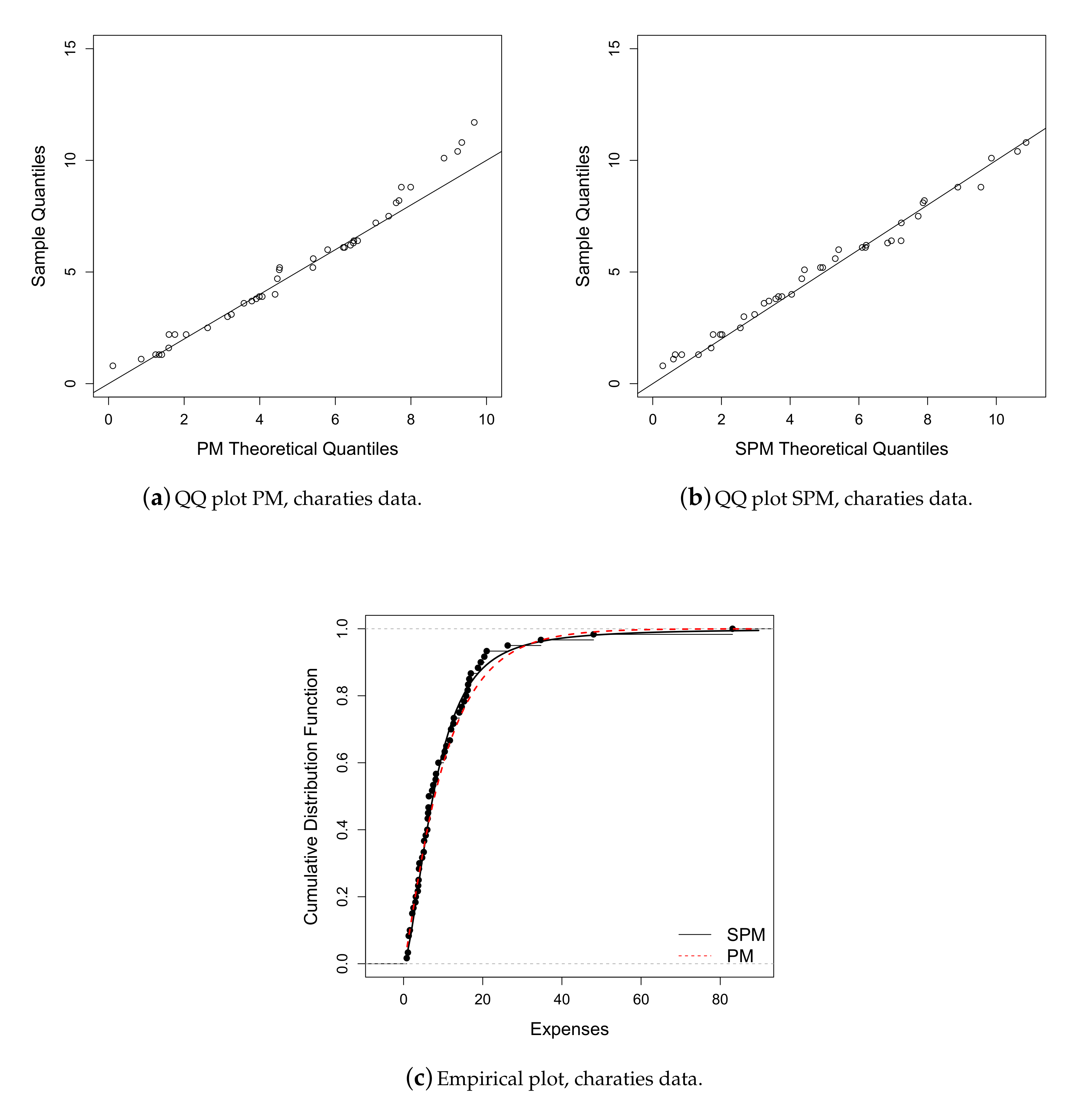
Figure 6.
QQ and empirical plot, charaties data.

Figure 7.
Histogram of the copper data fitted with the M, PM and SPM distributions.

Figure 8.
QQ and empirical plot, copper data.


Table 1.
Tails comparison for different values for parameters of the SPM and PM (1.5, 1.5) distributions.
Table 1.
Tails comparison for different values for parameters of the SPM and PM (1.5, 1.5) distributions.
| Distributions | ||||
|---|---|---|---|---|
| PM (1.5, 1.5) | ||||
| SPM (1.5, 1.5, 10) | ||||
| SPM (1.5, 1.5, 5) | ||||
| SPM (1.5, 1.5, 3) | ||||
| SPM (1.5, 1.5, 1) |
Table 2.
Asymmetry and kurtosis values for the SPM distribution.
| q | |||
|---|---|---|---|
| 188.415 | |||
| 2 | 479.077 | ||
| 10 | 767.271 | ||
| 1000 | 789.663 | ||
| 36.686 | |||
| 2 | 81.509 | ||
| 10 | 144.018 | ||
| 1000 | 149.444 | ||
| 5 | 2.397 | 19.256 | |
| 2 | 2.670 | 35.360 | |
| 10 | 4.482 | 70.302 | |
| 1000 | 4.648 | 73.800 | |
| 7 | 9.480 | ||
| 2 | 8.844 | ||
| 10 | 25.013 | ||
| 1000 | 27.857 | ||
| 9 | 8.079 | ||
| 2 | 5.081 | ||
| 10 | 16.444 | ||
| 1000 | 19.755 | ||
| 10 | 7.791 | ||
| 2 | 4.360 | ||
| 10 | 14.224 | ||
| 1000 | 17.828 |
Table 3.
Values of mean, variance, median and mode.
| Parameters | Mean | Variance | Median | Mode |
|---|---|---|---|---|
| 2.378 | 2.519 | 2.071 | 1.847 | |
| 1.391 | 0.862 | 1.211 | 1.080 | |
| 1.104 | 0.543 | 0.961 | 0.857 | |
| 1.500 | 2.750 | 1.075 | 0.415 | |
| 1.391 | 0.862 | 1.211 | 1.080 | |
| 1.428 | 0.742 | 1.225 | 1.099 | |
| 1.770 | 16.439 | 1.330 | 1.109 | |
| 1.391 | 0.862 | 1.211 | 1.080 | |
| 1.236 | 0.336 | 1.142 | 1.057 | |
| 1.192 | 0.256 | 1.119 | 1.048 |
Table 4.
Mean of each maximum likelihood (ML) estimate with standard deviations in parentheses.
| n | ||||
|---|---|---|---|---|
| 50 | ||||
| 100 | ||||
| 200 | ||||
| 50 | ||||
| 100 | ||||
| 200 | ||||
| 50 | ||||
| 100 | ||||
| 200 | ||||
| 50 | ||||
| 100 | ||||
| 200 | ||||
| 50 | ||||
| 100 | ||||
| 200 | ||||
| 50 | ||||
| 100 | ||||
| 200 |
Table 5.
SPM simulation, criteria comparison.
| AIC | BIC | ADR | AD2R | ||||||
|---|---|---|---|---|---|---|---|---|---|
| SPM | PM | SPM | PM | SPM | PM | SPM | PM | ||
| 50 | 0.627 | 0.373 | 0.479 | 0.521 | 0.804 | 0.196 | 0.999 | 0.001 | |
| 100 | 0.863 | 0.137 | 0.772 | 0.228 | 0.801 | 0.199 | 1.000 | 0.000 | |
| 200 | 0.993 | 0.007 | 0.970 | 0.030 | 0.798 | 0.202 | 1.000 | 0.000 | |
| 50 | 0.643 | 0.357 | 0.501 | 0.499 | 0.777 | 0.223 | 1.000 | 0.000 | |
| 100 | 0.874 | 0.126 | 0.758 | 0.242 | 0.768 | 0.232 | 1.000 | 0.000 | |
| 200 | 0.982 | 0.018 | 0.952 | 0.048 | 0.794 | 0.206 | 1.000 | 0.000 | |
| 50 | 0.432 | 0.568 | 0.303 | 0.697 | 0.804 | 0.196 | 0.998 | 0.002 | |
| 100 | 0.681 | 0.319 | 0.539 | 0.461 | 0.783 | 0.217 | 1.000 | 0.000 | |
| 200 | 0.899 | 0.101 | 0.762 | 0.238 | 0.795 | 0.205 | 0.999 | 0.001 | |
| 50 | 0.993 | 0.007 | 0.992 | 0.008 | 0.539 | 0.461 | 0.999 | 0.001 | |
| 100 | 1.000 | 0.000 | 1.000 | 0.000 | 0.502 | 0.498 | 1.000 | 0.000 | |
| 200 | 1.000 | 0.000 | 1.000 | 0.000 | 0.453 | 0.547 | 0.976 | 0.024 | |
| 50 | 0.880 | 0.120 | 0.862 | 0.138 | 0.630 | 0.370 | 0.997 | 0.003 | |
| 100 | 0.980 | 0.020 | 0.980 | 0.020 | 0.629 | 0.371 | 1.000 | 0.000 | |
| 200 | 0.998 | 0.002 | 0.996 | 0.004 | 0.587 | 0.413 | 0.980 | 0.020 | |
Table 6.
Descriptive analysis for the charities data.
| Mean | S.D. | Median | Interquartile Range | Min. | Max. | Asymmetry | Kurtosis |
|---|---|---|---|---|---|---|---|
| 10.892 | 12.741 | 6.800 | 10.375 | 0.800 | 83.100 | 3.602 | 19.360 |
Table 7.
ML estimates for the charities data with standard deviations in parentheses.
| Parameter | M | PM | SPM |
|---|---|---|---|
| 0.005(0.0006) | 0.196(0.047) | 0.198(0.059) | |
| — | 0.436(0.039) | 0.563(0.080) | |
| q | — | — | 2.122(0.733) |
| l | 277.564 | 201.531 | 199.017 |
| AIC | 557.127 | 407.063 | 404.034 |
| BIC | 559.228 | 411.251 | 410.317 |
| ADR | 65.062 | 26.711 | 25.425 |
| AD2R | 2.752 × 10 | 2799.457 | 269.557 |
Table 8.
Descriptive analysis for the copper data.
| Mean | S.D. | Median | Interquartile Range | Min. | Max. | Asymmetry | Kurtosis |
|---|---|---|---|---|---|---|---|
| 3.666 | 1.612 | 3.300 | 1.75 | 2 | 10.1 | 2.760 | 11.689 |
Table 9.
ML estimates for the copper data with standard deviations in parentheses.
| Parameter | M | PM | SPM |
|---|---|---|---|
| 0.094(0.015) | 0.097(0.043) | 0.006(0.005) | |
| — | 0.989(0.130) | 2.704(0.517) | |
| q | — | — | 3.591(1.083) |
| l | −42.193 | −42.190 | −34.567 |
| AIC | 86.386 | 88.380 | 75.135 |
| BIC | 87.564 | 90.736 | 78.670 |
| ADR | 0.762 | 0.753 | 0.106 |
| AD2R | 160.036 | 138.239 | 2.061 |
© 2020 by the authors. Licensee MDPI, Basel, Switzerland. This article is an open access article distributed under the terms and conditions of the Creative Commons Attribution (CC BY) license (http://creativecommons.org/licenses/by/4.0/).
Share and Cite
MDPI and ACS Style
Segovia, F.A.; Gómez, Y.M.; Venegas, O.; Gómez, H.W. A Power Maxwell Distribution with Heavy Tails and Applications. Mathematics 2020, 8, 1116. https://doi.org/10.3390/math8071116
AMA Style
Segovia FA, Gómez YM, Venegas O, Gómez HW. A Power Maxwell Distribution with Heavy Tails and Applications. Mathematics. 2020; 8(7):1116. https://doi.org/10.3390/math8071116
Chicago/Turabian StyleSegovia, Francisco A., Yolanda M. Gómez, Osvaldo Venegas, and Héctor W. Gómez. 2020. "A Power Maxwell Distribution with Heavy Tails and Applications" Mathematics 8, no. 7: 1116. https://doi.org/10.3390/math8071116
Note that from the first issue of 2016, this journal uses article numbers instead of page numbers. See further details here.